Fermi condensates for dynamic imaging of electro-magnetic fields

Abstract

Ultracold gases provide micrometer size atomic samples whose sensitivity to external fields may be exploited in sensor applications. Bose-Einstein condensates of atomic gases have been demonstrated to perform excellently as magnetic field sensors Wildermuth et al. (2005) in atom chip Folman et al. (2002); Fortágh and Zimmermann (2007) experiments. As such, they offer a combination of resolution and sensitivity presently unattainable by other methods Wildermuth et al. (2006). Here we propose that condensates of Fermionic atoms can be used for non-invasive sensing of time-dependent and static magnetic and electric fields, by utilizing the tunable energy gap in the excitation spectrum as a frequency filter. Perturbations of the gas by the field create both collective excitations and quasiparticles. Excitation of quasiparticles requires the frequency of the perturbation to exceed the energy gap. Thus, by tuning the gap, the frequencies of the field may be selectively monitored from the amount of quasiparticles which is measurable for instance by RF-spectroscopy. We analyse the proposed method by calculating the density-density susceptibility, i.e. the dynamic structure factor, of the gas. We discuss the sensitivity and spatial resolution of the method which may, with advanced techniques for quasiparticle observation Schirotzek et al. (2008), be in the half a micron scale.

The density of an ultracold alkali gas is sensitive to spatially varying magnetic fields due to the Zeeman effect. This is the principle behind magnetic trapping: atoms in low field seeking states are trapped at the minima of the field. On the other hand, it can be used for sensing since magnetic perturbations leave marks on the density of the gas. Such magnetic field imaging has been experimentally demonstrated with Bose-Einstein condensates in microtraps Wildermuth et al. (2005, 2006). The microkelvin sample of atoms is magnetically trapped at about 5-200 µm distance from the room temperature chip surface. Any additional perturbing magnetic field $\delta B$ will displace the center of the trapping potential and this can be measured by absorption imaging, either in situ or after ballistic expansion. The change in the trapping potential $V$ is directly proportional to the additional field, i.e. $\delta V\propto\delta B$. Similarly, electric fields can be sensed using the Stark effect, $\delta V\propto\delta E$ Wildermuth et al. (2006). The principle of using density perturbations of an ultracold atomic gas for sensing can be extended, for instance, to gases that are trapped optically, that are not on atom chips but brought in the vicinity of the sample by other means, or that consist of fermionic atoms instead of bosons. We propose to utilize the pairing gap present in a fermionic superfluid for temporally and spatially resolved imaging of magnetic (or electric) fields. Superfluids of Fermi gases have been recently observed, for reviews see e.g. Bloch et al. (2008); Giorgini et al. (2007). Also degenerate Fermi gases in microtraps have been realized Aubin et al. (2006).

In the proposed method, the Fermi condensate is trapped, magnetically or optically, near the sample of interest. Magnetic fields in the sample, generated for instance by electric currents or even spin, cause density perturbations to the Fermi gas. The perturbations, providing energy and momentum to the gas, lead to collective or quasiparticle excitations. The sensing is initiated by having a high value for the excitation gap $\Delta$. Only frequencies above $2\Delta$ will be able to break pairs. The gap $\Delta$ can be controlled with a Feshbach resonance (or by changing the density). Gradually changing the gap allows the isolation of individual frequencies: every time $2\Delta$ crosses a frequency present in the magnetic field, the measured amount of quasiparticle excitations increases abruptly, see Figures 1 and 3. The quasiparticles can be detected by RF-spectroscopy Regal and Jin (2003); Gupta et al. (2003); Chin et al. (2004); Kinnunen et al. (2004).

For spatial imaging of static fields, the following variant of the method can be used: The spatial dependence of the static perturbation provides momenta for the gas but no energy. Energy is given by modulating the gas uniformly in space, with a frequency corresponding to the pair breaking. In other words, the static perturbations serve as nucleation centers for quasiparticles under time-periodic modulation.

Within linear response, the density response is

$$\delta\rho(\mathbf{q},\omega)=\chi(\mathbf{q},\omega)\delta V(\mathbf{q},\omega),$$ (1)

where we calculate the susceptibility $\chi$ with the generalized random phase approximation, following Côté and Griffin (1993). We solve $\chi(\mathbf{q},\omega)$ numerically from the most general form given in Côté and Griffin (1993), without making the approximation of weak coupling strength. For the equation of state, see Methods. The magnetic field is taken to be of the form $B=\sum_{i}A_{i}\delta(\omega-\omega_{i})\varphi_{i}(\mathbf{q})$, where $A_{i}$ is the amplitude. The momentum part, $\varphi_{i}(\mathbf{q})$, is due to the geometry of the perturbation and we assume it is independent of frequency. Then

$$\delta\rho(\mathbf{q},\omega)=\chi(\mathbf{q},\omega)\varphi(\mathbf{q})\sum_{i}A_{i}\delta(\omega-\omega_{i}).$$ (2)

All the relevant information is embedded in $\chi(\mathbf{q},\omega)$, or rather its imaginary part, the dynamic structure factor: $S(\mathbf{q},\omega)=-1/\pi\text{Im}\chi(\mathbf{q},\omega)$. The dynamic structure factor has two parts: Anderson-Bogoliubov (AB) phonon which is a collective mode with frequency below $2\Delta$, and quasiparticle excitations with frequencies above $2\Delta$, see Figure 2. The results are in qualitative agreement with those in Côté and Griffin (1993); Minguzzi et al. (2001); Büchler et al. (2004); Combescot et al. (2006); Bruun and Baym (2006); Challis et al. (2007); Veeravalli et al. (2008).

The strong dependence of the qualitative behaviour of the dynamic structure factor on momentum, Figure 2, allows to focus on perturbations of a chosen length scale. The AB-phonon, or the collective modes of a harmonically trapped gas, may be used for detecting spatially large scale perturbations. Here we concentrate on perturbations of small size ($1/q\sim 1/(2k_{F})$) which cause a strong quasiparticle response near and above the pair breaking frequencies. For sizes smaller than $1/(2k_{F})$ the quasiparticle threshold loses its dependence on $\Delta$ and approaches the free particle dispersion $\omega\propto q^{2}$.

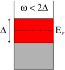
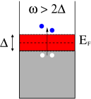
Figure 1: A Fermi condensate is trapped near the sample of interest. A gap opens around the Fermi level of the superfluid and sets the minimum energy of single particle excitations to the value of the order parameter, $\Delta$. Magnetic fields with certain frequency and location in the sample cause density perturbations in the condensate. Only if the frequency exceeds $2\Delta$, quasiparticles are created, which allows sensing perturbations of different frequencies by tuning the gap.

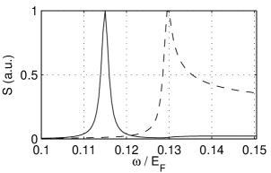
Figure 2: Dynamic structure factor $S$ as a function of frequency, with two momenta, $q=0.2k_{F}$ (solid line) and $q=0.4k_{F}$ (dashed line). The smaller momentum case shows the AB phonon as a clear peak, and the quasiparticle continuum above $\omega=2\Delta\approx 0.13$, whereas when $q$ approaches $k_{F}$ the phonon merges with the quasiparticle continuum. Both curves are scaled to unity for readability.

In Figure 3 we show the response for different values of the gap $\Delta$, in a case where the perturbation contains four different frequencies, with $A_{i}=1$ for all (see Eq. (2)). The response is the sum of dynamic structure factors for the four frequencies. The frequencies show up as prominent features in the amount of quasiparticles when the gap is varied. Note that for both momenta ($0.4k_{F}$, $1k_{F}$), the peaks caused by quasiparticle formation are very similar. Thus for a realistic perturbation geometry, whose Fourier transform contains several momenta, the signal should still be well resolved as long as the perturbation is roughly of the size $1/k_{F}$.

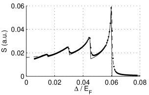
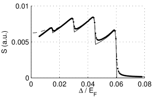
Figure 3: Dynamic structure factor as a function of the pairing gap, summed for four frequencies, $0.03$, $0.06$, $0.09$, and $0.12$, with two different momenta, $0.4k_{F}$ (left) and $1k_{F}$ (right). This corresponds to the amount of quasiparticles caused by a perturbing field with these four frequencies. The solid line shows the data with the AB phonon suppressed: for the momenta considered, the dynamic structure factor mainly corresponds to quasiparticle creation as the solid line closely follows the full result. The dashed line shows the result at a finite temperature, $T=0.01E_{F}$, which is of the order $0.5T_{c}$ for the $\Delta$ considered.

The amount of quasiparticles can be measured by applying RF-pulse(s) at zero and/or negative detunings (see Methods). The gases are typically confined by a harmonic potential, therefore the density and the gap are not uniform throughout the gas. Figure 4 shows that the threshold type behaviour disappears when the trapping potential has been taken into account by local density approximation (see Methods), but the frequency of the perturbation is still visible as a maximum. However, we found that such smoothened response allows to isolate only a few, not very closely spaced, frequencies, unlike in the homogenous case.

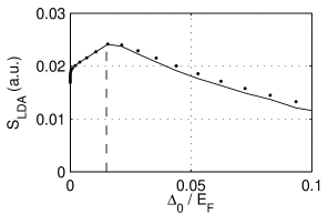
Figure 4: The dynamic structure factor for a single frequency $\omega=0.03$ and $q=1k_{F}$ , averaged for a harmonic confinement using LDA, as a function of the gap at the center of the trap $\Delta_{0}$. Since the pairing gap is always small at the edges of the trap, there is a finite response already for $\Delta_{0}>\omega_{0}/2$. Decreasing $\Delta_{0}$ allows quasiparticle creation in larger areas in the trap, increasing the response, but once the quasiparticles can be formed also at the center of the trap, such growth stops. This leads to a maximum of the response at $\Delta_{0}=\omega_{0}/2$, shown by the vertical dashed line.

With tomographic techniques Shin et al. (2007); Schirotzek et al. (2008), the RF-spectroscopy can be spatially resolved in three dimensions. In our proposed method, spatially resolved RF-spectroscopy could be used for accurate determination (without smoothening by the trap-averaging) of the perturbation frequencies and, naturally, for resolving the perturbation spatially (also in the static version of the method). Furthermore, the non-uniform density profile of the trapped gas simultaneously provides experiments with different gap values, which could be utilized when the perturbation is, e.g., a long thin wire.

The frequencies that can at the present be resolved with the method are limited by the experimentally demonstrated gap values to the order of 10 kHz. At the unitarity limit, the gap becomes proportional to the Fermi energy, thereby higher particle numbers allow higher frequencies. Within linear response, which is proportional to $|\delta Vt|^{2}$, the sensitivity is basically given by the time available for the measurement. We estimate the sensitivity to be $10^{-8}-10^{-12}$ Tesla (see Methods). To detect a single spin, the maximum distance of the gas from the surface is estimated to be about $\sim 0.5$ µm which is not possible due to noise and heating of the gas for samples at room temperature Folman et al. (2002) but may be for those at cryogenic temperatures Verdu et al. (2008); Dikovsky et al. (2008) or for ones utlilizing photonic band gap materials Bravo-Abad et al. (2006). Using Feshbach resonances, the gas of Fermions can be also converted into a Bose-Einstein condensate of molecules Jochim et al. (2003); Regal et al. (2003). Thereby, a setup used for the Fermi condensate sensor proposed here could be easily turned into one that functions as the Bose-Einstein condensate sensor Wildermuth et al. (2005, 2006) as well, only with double mass of the particles which increases the sensitivity.

At the present, several other systems than BCS-type superfluids are being pursued with ultracold gases: the proposed method could be extended to other gapped systems and thereby to new frequency ranges. This could also allow higher spatial resolution: Quite naturally, the spatial resolution of a response that involves interparticle correlations is given by the interparticle distance $1/k_{F}$, which for typical trapped Fermi gases is about $1/(2k_{F})\sim 0.5\mu m$ as discussed above. It can, however, be smaller in optical lattices Lewenstein et al. (2007); Bloch et al. (2008) and, especially, the self-assembled crystals of ultracold polar molecules proposed in Büchler et al. (2007) could offer interparticle distances and thus resolutions in the nanometer scale.

In summary, we have proposed to use an ultracold Fermi gas in a gapped state as a sensor for time-dependent and static magnetic fields. The tunable gap works as a frequency filter, and the locations of the perturbation act as nucleation centers for quasiparticles measurable with RF-spectroscopy.

I Methods

We assume a two-component (pseudospins $\uparrow$ and $\downarrow$) Fermi gas in a superfluid state described by the standard Bardeen-Cooper-Schrieffer (BCS) theory, given by the Hamiltonian

$$H=\sum_{\mathbf{k}}(\epsilon_{\mathbf{k}}-\mu)(c_{\uparrow\mathbf{k}}^{\dagger}c_{\uparrow\mathbf{k}}+c_{\downarrow\mathbf{k}}^{\dagger}c_{\downarrow\mathbf{k}})+\Delta c_{\uparrow\mathbf{k}}^{\dagger}c_{\downarrow-\mathbf{k}}^{\dagger}+\Delta c_{\downarrow-\mathbf{k}}c_{\uparrow\mathbf{k}}.$$ (3)

The order parameter $\Delta$ and the chemical potential $\mu$ are obtained by iteratively solving the self-consistent crossover equations

$$1=\frac{2|k_{F}a|}{\pi}\int_{0}^{k_{C}}\frac{k^{2}(1-2n_{F}(E_{k}))}{E_{k}}-1\,dk$$ (4)

and

$$1=\frac{3}{2}\int_{0}^{k_{C}}\left(\frac{k^{2}-\mu}{E_{k}}(2n_{F}(E_{k})-1)+1\right)k^{2}\,dk,$$ (5)

where $E_{k}=\sqrt{(k^{2}-\mu)^{2}+\Delta^{2}}$ is the BCS quasiparticle dispersion, $n_{F}(\epsilon)=1/(1+e^{\beta\epsilon})$ is the Fermi function, $k_{C}$ is the cut-off, and $k_{F}a$ is the dimensionless coupling constant.

We use interactions parameters in range $0>k_{F}a>-0.66$, resulting in pairing gaps $\Delta$ up to $0.1E_{F}$. All our calculations are at zero temperature except the dashed line in Figure 3. We the maximum used $k_{F}a=-0.66$ which is in the BSC limit just in order to be able to do the finite temperature calculation within simple BCS theory. The method itself is by no means limited to weak interactions, and actually all the estimates about the performance (frequencies, sensitivities, etc.) are done assuming that the experiments are done at the unitarity limit. Note that while the AB phonon is a signature of superfluidity, the quasiparticle creation does not require a superfluid. Therefore a gas at temperatures above $T_{c}$ but having a pseudogap Chen et al. (2005) could serve as well but the response would be smoothened due to the lack of sharp features in the density of states Chen et al. (2005); Bruun and Baym (2006).

To detect the quasiparticles, RF pulses transferring atoms in one of the components $\uparrow$ or $\downarrow$ to a third internal state are applied with zero and/or negative detunings (or positive if there are strong Hartree contributions Schirotzek et al. (2008)), avoiding detunings which would break pairs. In this way only the quasiparticles produced by the magnetic field perturbation are observed. Note that the RF pulse length can be rather short, increasing the operation speed of the sensor, since high energy resolution is not required; actually it can be an advantage if the pulse samples several negative/zero detunings simultaneously via the large linewidth. The quasiparticle response could be calibrated by experiments with known perturbations, e.g. microfabricated current carrying structures. Moreover, the static structure factor of a Fermi gas can be measured by Bragg spectroscopy Veeravalli et al. (2008) which is also be useful for calibration.

In order to account for the effects caused by the harmonic trapping, we have used the local density approximation (LDA) to average the signal over the trap. One defines a local chemical potential

$$\mu(r)=\mu_{0}-\frac{1}{2}m\omega^{2}r^{2},$$ (6)

where $\mu_{0}$ is the chemical potential at the center of the trap, and calculates $S(\mu(r))$ at distance $r$ as for a uniform system. The result is given by

$$\begin{split}S_{\text{LDA}}\propto&\int_{0}^{\infty}S(\mu(r))r^{2}\,dr\\ =&\frac{1}{2}\left(\frac{2\mu_{0}}{m\omega^{2}}\right)^{\frac{3}{2}}\int_{-\infty}^{1}\sqrt{1-\mu}S(\mu)\,d\mu,\end{split}$$ (7)

where $\mu$ is in the units of $\mu_{0}$. Note that this reasoning assumes perturbations spanning the whole gas. One or a few localized centers would again give sharp response, without the need for such trap-averaging, however, there would be ambiguity in determination of $\omega$ if the location of the center is not resolved too. The final state momentum-resolved RF-spectroscopy Stewart et al. (2008) could be useful in this context.

When estimating the time available for the experiment, one should consider not only the lifetime of the gas which can be easily $100$ ms - $1$ s or even longer, but also the diffusion time of quasiparticles if high spatial resolution is aimed at. According to the measurements in Shin et al. (2007), no significant diffusion happened during $5$ ms. Therefore we take $10$ ms and $1$ s as the lower and upper bounds for the time available when estimating the sensitivity.

The probability for producing an excitation with potential energy $V$ applied for duration $\tau$ is proportional to $|V\tau/h|^{2}$. Assuming the probability needed for a detectable signal (minimum number of excited particles) is at best $0.01$ and at worst $1$, the minimum potential energy $V$ is between $0.1h/\tau$ and $h/\tau$. With the $10$ ms - $1$ s time scales given above the potential energy sensitivity lies between $h\cdot 0.1$ Hz and $h\cdot 100$ Hz $\equiv h\nu$.

The potential experienced by a neutral atom in the hyperfine state $m_{F}$ is $V=g\mu_{\text{B}}m_{F}B$, where $\mu_{0}$ is the vacuum permeability, $\mu_{\text{B}}=e\hbar/2m$ is the Bohr magneton, and $g\approx 2$ is the Landé factor. Therefore, assuming that the potential energy sensitivity is $h\nu$, the magnetic field sensitivity is $h\nu/2\mu_{B}m_{F}\approx 3.6\cdot 10^{-11}$ T/Hz for $m_{F}=9/2$. With the limits for $\nu$ given above, the sensitivity is between $10^{-12}$ and $10^{-8}$ T.

Detection of a single spin is in principle possible. The magnitude of the magnetic field due to the spin of an electron is approximately $B(r)=\mu_{0}\mu_{\text{B}}g/4\pi r^{3}$, where $\mu_{0}$ is the vacuum permeability, and $r$ is the distance from the electron. Therefore the required sensitivity to be able to detect a single spin has an upper bound of

$$\delta V=\frac{\mu_{0}\mu_{\text{B}}m_{F}}{\pi r^{3}}.$$ (8)

Conversely, assuming the potential energy sensitivity of $h\cdot 1$ Hz (from our estimated range of $0.1$ - $100$ Hz), the maximum distance at which the detection is possible is $\left(\mu_{0}\mu_{\text{B}}m_{F}/h\pi\text{Hz}\right)^{\frac{1}{3}}\approx 0.6$ µm for $m_{F}=9/2$.

II Acknowledgements

We thank J. Hecker Denschlag for useful discussions. This work was supported by the National Graduate School in Materials Physics, Ellen and Artturi Nyyssönen foundation, Academy of Finland (Project Nos. 213362, 217045, 217041, 217043) and conducted as a part of a EURYI scheme award. See www.esf.org/euryi.

References

- Wildermuth et al. (2005) S. Wildermuth, S. Hofferberth, I. Lesanovsky, E. Haller, L. Andersson, S. Groth, I. Bar-Joseph, P. Kr uger, and J. Schmiedmayer, Nature 435, 440 (2005).
- Folman et al. (2002) R. Folman, P. Krüger, J. Schmiedmayer, J. Denschlag, and C. Henkel, Adv. At. Mol. Opt. Phys. 48, 263 (2002).
- Fortágh and Zimmermann (2007) J. Fortágh and C. Zimmermann, Rev. Mod. Phys. 79, 235 (2007).
- Wildermuth et al. (2006) S. Wildermuth, S. Hofferberth, I. Lesanovsky, S. Groth, P. Krüger, and J. Schmiedmayer, Appl. Phys. Lett. 88, 264103 (2006).
- Schirotzek et al. (2008) A. Schirotzek, Y.-I. Shin, C. H. Schunck, and W. Ketterle (2008), eprint arXiv:0808.0026.
- Bloch et al. (2008) I. Bloch, J. Dalibard, and W. Zwerger, Rev. Mod. Phys. 80, 885 (2008).
- Giorgini et al. (2007) S. Giorgini, L. Pitaevskii, and S. Stringari (2007), eprint arXiv:0706.3360.
- Aubin et al. (2006) S. Aubin, S. Myrskog, M. Extavour, L. LeBlanc, D. McKay, A. Stummer, and J. Thywissen, Nature Physics 2, 384 (2006).
- Regal and Jin (2003) C. A. Regal and D. S. Jin, Phys. Rev. Lett. 90, 230404 (2003).
- Gupta et al. (2003) S. Gupta, Z. Hadzibabic, M.W.Zwierlein, C. Stan, K. Dieckmann, C. Schunck, E. van Kempen, B. Verhaar, and W. Ketterle, Science 300, 1723 (2003).
- Chin et al. (2004) C. Chin, M. Bartenstein, A. Altmeyer, S. Riedl, S. Jochim, J. H. Denschlag, and R. Grimm, Science 305, 1128 (2004).
- Kinnunen et al. (2004) J. Kinnunen, M. Rodriguez, and P. Törmä, Science 305, 1131 (2004).
- Côté and Griffin (1993) R. Côté and A. Griffin, Phys. Rev. B 48, 10404 (1993).
- Minguzzi et al. (2001) A. Minguzzi, G. Ferrari, and Y. Castin, Eur. Phys. J. D 17, 49 (2001).
- Büchler et al. (2004) H. P. Büchler, P. Zoller, and W. Zwerger, Phys. Rev. Lett 93, 080401 (2004).
- Combescot et al. (2006) R. Combescot, S. Giorgini, and S. Stringari, Europhys. Lett. 75, 695 (2006).
- Bruun and Baym (2006) G. M. Bruun and G. Baym, Phys. Rev. A 74, 033623 (2006).
- Challis et al. (2007) K. J. Challis, R. J. Ballagh, and C. W. Gardiner, Phys. Rev. Lett. 98, 093002 (2007).
- Veeravalli et al. (2008) G. Veeravalli, E. Kuhnle, P. Dyke, and C. J. Vale (2008), eprint arXiv:0809.2145.
- Shin et al. (2007) Y. Shin, C. H. Schunck, A. Schirotzek, and W. Ketterle, Phys. Rev. Lett. 99, 090403 (2007).
- Verdu et al. (2008) J. Verdu, H. Zoubi, C. Koller, J. Majer, H. Ritsch, and J. Schmiedmayer (2008), eprint arXiv:0809.2552.
- Dikovsky et al. (2008) V. Dikovsky, V. Sokolovsky, B. Zhang, C. Henkel, and R. Folman (2008), eprint arXiv:0808.1897.
- Bravo-Abad et al. (2006) J. Bravo-Abad, M. Ibanescu, J. D. Joannopoulos, and M. Soljacic, Physical Review A 74, 053619 (2006).
- Jochim et al. (2003) S. Jochim, M. Bartenstein, A. Altmeyer, G. Hendl, S. Riedl, C. Chin, J. H. Denschlag, and R. Grimm, Science 302, 2101 (2003).
- Regal et al. (2003) C. Regal, M. Greiner, and D. Jin, Nature 426, 537 (2003).
- Lewenstein et al. (2007) M. Lewenstein, A. Sanpera, V. Ahufinger, B. Damski, A. S. De, and U. Sen, Adv. Phys. 56, 243 (2007).
- Büchler et al. (2007) H. P. Büchler, E. Demler, M. Lukin, A. Micheli, N. Prokof’ev, G. Pupillo, and P. Zoller, Phys. Rev. Lett. 98, 060404 (2007).
- Chen et al. (2005) Q. Chen, J. Stajic, S. Tan, and K. Levin, Phys. Rep. 412, 1 (2005).
- Stewart et al. (2008) J. T. Stewart, J. P. Gaebler, , and D. S. Jin, Nature 454, 744 (2008).