Subdiffusive motion in kinetically constrained models

Abstract

We discuss a kinetically constrained model in which real-valued local densities fluctuate in time, as introduced recently by Bertin, Bouchaud and Lequeux. We show how the phenomenology of this model can be reproduced by an effective theory of mobility excitations propagating in a disordered environment. Both excitations and probe particles have subdiffusive motion, characterised by different exponents and operating on different time scales. We derive these exponents, showing that they depend continuously on one of the parameters of the model.

I Introduction

There has been considerable recent interest in the hypothesis that glassy materials can be described by coarse-grained models with simple thermodynamic properties and non-trivial kinetic constraints RitortS03 ; GarrahanC02 ; JungGC04 ; BBL05 ; BGC-Fick ; Chandler06 ; knights ; Berthier-chi4 These models capture the dynamically heterogeneous nature of glass-formers DHReviews : the implicit assumption is that microscopic details of the glass-former are important only insofar as they set the parameters of the coarse-grained dynamical theory. Some kinetically constrained models describe particles hopping on a lattice KA ; TLG ; in other cases, binary (Ising) spins are used GarrahanC02 ; FredricksonA84 ; EisingerJ93 , where the two states of the spin represent ‘mobile’ and ‘immobile’ regions of the liquid.

In a recent paper, Bertin, Bouchaud and Lequeux (BBL) BBL05 discussed a kinetically constrained model in which molecular degrees of freedom are modeled by a real-valued local density, defined on a lattice. Loosely speaking, regions of high density correspond to immobile sites in the spin description of FredricksonA84 , and regions of low density correspond to mobile sites. However, the continuous range of densities in the BBL model captures the fact that a glass-forming system has a variety of local packings, which may not permit a simple decomposition into mobile and immobile. The continuous range of densities leads to a continuous range of mobilities, resulting in a very broad distribution of relaxation times, characteristic of glassy behaviour.

As discussed in Ref. BBL05 , relaxation in the BBL model occurs by means of ‘mobility excitations’ that propagate subdiffusively across the system. Links between broadly distributed relaxation times and subdiffusive motion of particles are quite familiar in theories of glass-forming liquids trap . Here, we focus initially on the motion of mobility excitations, by coarse-graining the BBL model onto an effective theory for these excitations. This procedure represents a very simple example of the coarse-graining of glassy materials that was proposed by Garrahan and Chandler GarrahanC02 . The resulting effective theory is a disordered generalisation of the one-spin facilitated Fredrickson-Andersen (FA) model FredricksonA84 . The possibility of subdiffusive motion in this model is important when comparing model results with experiments on supercooled liquids: on approaching the experimental glass transition time scales increase dramatically, while the length scales associated with dynamical heterogeneity grow more slowly DHReviews ; Qiu03 ; Berthier-expt-long . In the dynamical facilitation picture GarrahanC02 , the motion of mobility excitations leads to a relation of the form $\tau\sim\xi^{z}/\Omega$ where $z$ is a dynamical exponent, $\tau$ the relaxation time scale, $\xi$ the length scale associated with dynamical heterogeneity, and $\Omega$ a (possibly temperature dependent) constant Whitelam04 . Subdiffusion of these excitations corresponds to an exponent $z>2$, consistent with a time scale that increases much more quickly with the corresponding length scale than for ordinary diffusion.

In this paper we focus throughout on the one-dimensional case, where subdiffusion effects are most pronounced BBL05 . Analysis of the disordered FA model leads us to two main results. Firstly, we are able to explain the scaling exponents observed in BBL05 . In particular, while the disorder in both the BBL and disordered FA models is fluctuating, we explain why excitations propagate with the scaling laws expected for a particle moving in a quenched random environment. Secondly, we consider the motion of probe particles in the BBL and disordered FA models. These particles propagate subdiffusively, but with scaling laws that are different from those of the mobility excitations.

The form of the paper is as follows. In section II, we define the BBL model and the disordered FA model. In section III, we use four-point correlation functions Berthier-chi4 ; FranzDPG99 ; Berthier04 ; ToninelliWBBB05 to investigate the subdiffusive propagation of mobility excitations, and we discuss the associated scaling exponents. In section IV, we consider the motion of probe particles in the BBL model, and show that this behaviour can also be reproduced in the disordered FA model.

II Models

II.1 BBL model

The (one-dimensional) BBL model is defined BBL05 for a chain of continuous densities $\{\rho_{i}\}$, constrained to $0<\rho_{i}<2$. Dynamical moves involve rearrangement of the density between adjacent pairs of sites:

$$\rho_{i},\rho_{i+1}\to\rho_{i}^{\prime},\rho_{i+1}^{\prime},\quad\hbox{rate }f_{i}P_{\rho}(\rho_{i}^{\prime},\rho_{i+1}^{\prime}|\rho_{i}+\rho_{i+1}),$$ (1)

where $f_{i}=\Theta(2-\rho_{i}-\rho_{i+1})$ is the facilitation function for bond $i$, between sites $i$ and $i+1$. Here, $\Theta(x)$ is the Heaviside step function, so a density rearragement between two sites can occur only if the total density on those sites is less than two. The distribution of densities after the rearrangement is

$$P_{\rho}(\rho_{i},\rho_{i+1}|R)=A(\rho_{i}\rho_{i+1})^{\mu-1}\delta(R-\rho_{i}-\rho_{i+1}),$$ (2)

where the delta function enforces volume conservation. The parameter $\mu>0$ was motivated in BBL05 in terms of an interaction between the particles of the model. If $\mu>1$ then the density after the rearrangment tends to be distributed equally between sites $i$ and $i+1$; if $\mu<1$ then the density is more likely to accumulate on just one of the sites. The coefficient $A=[R^{1-2\mu}\Gamma(2\mu)/\Gamma(\mu)^{2}]$ is determined by the requirement that

$$\int_{0}^{2}\!\mathrm{d}\rho_{i}\int_{0}^{2}\!\mathrm{d}\rho_{i+1}\,P_{\rho}(\rho_{i},\rho_{i+1}|R)=1,$$ (3)

which means that all facilitated bonds rearrange with unit rate. [Here, $\Gamma(\mu)$ is the usual Gamma function.]

These dynamical rules respect detailed balance with respect to a steady state distribution $P_{\mathrm{stat,BBL}}(\{\rho_{i}\})$ that factorises between sites. In the grand canonical ensemble we have

$$P_{\mathrm{stat,BBL}}(\{\rho_{i}\})=\prod_{i}P_{\mathrm{s}}(\rho_{i}),\qquad P_{\mathrm{s}}(\rho)\propto\rho^{\mu-1}e^{\gamma\rho},$$ (4)

normalised so that $\int_{0}^{2}\!\mathrm{d}\rho\,P_{\mathrm{s}}(\rho)=1$. Our notation differs from BBL05 in that we use $\gamma$ for the Lagrange multiplier conjugate to density, reserving $\beta$ for the inverse temperature of the FA model.

It is clear from Eq. (1) that motion is only possible across bonds with $f_{i}=1$. We refer to these as facilitated bonds. The steady state contains a finite fraction of facilitated bonds, which we denote by

$$\eta\equiv\langle f_{i}\rangle.$$ (5)

We also define the mean density,

$$\overline{\rho}\equiv\langle\rho_{i}\rangle.$$ (6)

Facilitated bonds in the BBL model are the fundamental mobility excitations in the system. The interesting scaling limit is the one of maximal mean density, $\overline{\rho}\to 2$, where facilitated bonds are rare ($\eta\ll 1$). In this limit, $\gamma$ is large, and we have

$$\overline{\rho} = 2-\gamma^{-1}+\mathcal{O}(\gamma^{-2}),$$ (7)

$$\eta = 2\gamma\exp(-2\gamma)\frac{\Gamma(\mu)^{2}}{\Gamma(2\mu)}[1+\mathcal{O}(\gamma^{-1})]$$ (8)

consistent with BBL05 . It was further observed in BBL05 that the dynamics of these excitations in the BBL model can be represented schematically by the processes

$$01\leftrightarrow 11\leftrightarrow 10$$ (9)

where a 1 represents a facilitated bond ($f_{i}=1$ or $f_{i+1}=1$, respectively), and a $0$ an unfacilitated bond ($f_{i}=0$ or $f_{i+1}=0$). The above two-step process then produces effective diffusion of excitations. When excitations meet, they can coagulate via e.g. $101\to 111\to 011\to 010$; running through the steps in reverse, a single excitation can also branch into two. Excitations can never be created unless there is already an excitation present on a neighbouring bond, and this is the key motivation for the effective FA models presented below.

When excitations are rare, the rate-limiting step in the effective diffusion is the creation of a new excitation, $01\to 11$. To obtain the typical rate for this process, consider a density rearrangement event across bond $i+1$:

$$\rho_{i},\rho_{i+1},\rho_{i+2}\to\rho_{i},\rho_{i+1}^{\prime},\rho_{i+2}^{\prime}.$$ (10)

The process $01\to 11$ occurs when the second bond is facilitated in both initial and final states, while the first bond is facilitated only in the final state. That is,

$$\rho_{i+1}+\rho_{i+2}=\rho_{i+1}^{\prime}+\rho_{i+2}^{\prime} < 2,$$

$$\rho_{i}+\rho_{i+1} > 2,$$

$$\rho_{i}+\rho_{i+1}^{\prime} < 2.$$ (11)

To work out the typical rate with which these processes occur, we should perform a steady-state average over all initial configurations with the prescribed mobility configuration $(f_{i}=0,f_{i+1}=1)$, corresponding to the first two conditions listed. In addition, however, we condition on $\rho_{i}$, which strongly influences the rate if it is close to 2: the third condition given above can then only be met if $\rho_{i+1}^{\prime}$ is very small. Thus, we consider the average rate for the process $(\rho_{i}=2-\epsilon_{i},f_{i}=0,f_{i+1}=1)\to(\rho_{i}=2-\epsilon_{i},f_{i}=1,f_{i+1}=1)$, which can only occur via a density rearrangement across bond $i+1$ as written above. The steady-state distribution factorises between sites and so we have for this rate, denoted by $r_{i}(\rho_{i})$:

$$r_{i}(\rho_{i})=\frac{\int_{\epsilon_{i}}^{2}\!\mathrm{d}R\int_{\epsilon_{i}}^{R}\!\!\mathrm{d}\rho_{i+1}\,P_{\mathrm{s}}(\rho_{i+1})P_{\mathrm{s}}(R-\rho_{i+1})\int_{0}^{\epsilon_{i}}\mathrm{d}\rho^{\prime}_{i+1}\,\int_{0}^{2}\mathrm{d}\rho_{i+2}^{\prime}P_{\rho}(\rho_{i+1}^{\prime},\rho_{i+2}^{\prime}|R)}{\int_{\epsilon_{i}}^{2}\!\mathrm{d}R\int_{\epsilon_{i}}^{R}\!\!\mathrm{d}\rho_{i+1}\,P_{\mathrm{s}}(\rho_{i+1})P_{\mathrm{s}}(R-\rho_{i+1})}$$ (12)

where we have introduced $R=\rho_{i+1}+\rho_{i+2}$. The integral over $\rho_{i+2}^{\prime}$ in the numerator gives $A[\rho_{i+1}^{\prime}(R-\rho_{i+1}^{\prime})]^{\mu-1}$, and the one over $\rho_{i+1}^{\prime}$ then a normalized incomplete Beta function $B(\mu,\mu;\epsilon_{i}/R)/B(\mu,\mu)$. The remaining average over $R$ (and $\rho_{i+1}$) becomes concentrated around $R=2$ for large $\gamma$, so that in this limit

$$r_{i}(\epsilon_{i})=\frac{B(\mu,\mu;\epsilon_{i}/2)}{B(\mu,\mu)}=\frac{\int_{0}^{\epsilon_{i}/2}dv\,v^{\mu-1}(1-v)^{\mu-1}}{\int_{0}^{1}dv\,v^{\mu-1}(1-v)^{\mu-1}}$$ (13)

Recalling that the local density is $\rho_{i}=2-\epsilon_{i}$, we note that dense sites (those with small $\epsilon_{i}$) lead to small rates $r_{i}$.

The relaxation of the BBL model on long time scales is determined by sites with small $r_{i}$. For this reason, it is convenient to deduce the distribution of this rate from that of $\rho_{i}$, or equivalently $\epsilon_{i}$. From Eq. (4) one sees for large $\gamma$ that the variation of the power law factor $\rho^{\mu-1}$ near $\rho=2$ can be neglected, so that $P_{\mathrm{s}}(\epsilon_{i})=\gamma\exp(-\gamma\epsilon_{i})$. The typical values of $\epsilon_{i}$ are therefore small, $\epsilon_{i}\sim\gamma^{-1}$, and we can expand the rate as

$$r_{i}(\rho_{i})\simeq a\epsilon_{i}^{\mu},\qquad a=\frac{\Gamma(2\mu)}{\mu\,2^{\mu}\Gamma(\mu)^{2}}$$ (14)

Transforming then from the distribution of $\epsilon_{i}$ to $r_{i}$ gives

$$P_{\mathrm{s},r}(r) = \left[P_{\mathrm{s}}(\epsilon_{i})\left|\frac{\mathrm{d}r_{i}(\epsilon_{i})}{\mathrm{d}\epsilon_{i}}\right|^{-1}\right]_{r=r_{i}(\epsilon_{i})}$$ (15)

$$= \frac{1}{\mu\Omega_{0}}(r/\Omega_{0})^{(1/\mu)-1}\mathrm{e}^{-(r/\Omega_{0})^{1/\mu}}$$

where

$$\Omega_{0}=a\gamma^{-\mu}\sim\gamma^{-\mu}$$ (16)

is a microscopic rate, which acts as an upper cutoff on the distribution of rates. [The notation $u\sim v$ means that $u$ and $v$ are proportional to each other in the relevant limit (large $\gamma$).] It is important to note that the small-$r$ scaling of the distribution $P_{\mathrm{s},r}(r)\sim r^{(1/\mu)-1}$, which we derived above in the limit $\gamma\to\infty$, also applies at finite $\gamma$. This is because the rate for small $\epsilon_{i}$ always scales as in Eq. (14), and the probability density $P_{\mathrm{s}}(\epsilon_{i})$ of $\epsilon_{i}$ approaches a constant for small $\epsilon_{i}$ for all $\gamma$.

The long-time behaviour of the BBL model is now controlled by the behaviour of $P_{\mathrm{s},r}(r)$ at small $r$, and, in particular, by the exponent $\mu$. The time for a mobility excitation to diffuse across bond $i$ is of order $1/r_{i}$. The average diffusion time $\langle 1/r\rangle$, with the average taken over the distribution $P_{\mathrm{s},r}(r)$, then shows a change of behaviour at $\mu=1$: for $\mu<1$ it is finite, while for $\mu>1$ it diverges. This motivates why subdiffusion occurs in the second case: for arbitrarily long times $t$ there are a significant number of barriers to mobility diffusion that have transmission rate $<1/t$.

II.2 Effective FA model

We now describe the effective model that captures the dynamics of the mobile bonds on large length and time scales. In this model, the bonds of the BBL model are represented by a chain of binary variables $\{n_{i}\}$, where $n_{i}=1$ if the bond between sites $i$ and $i+1$ of the BBL model is mobile, and $n_{i}=0$ otherwise. The variable $n_{i}$ corresponds to the BBL variable $f_{i}$. The process of (9) is then

$$(n_{i}=0,n_{i+1}=1)\to(n_{i}=1,n_{i+1}=1).$$ (17)

It occurs with a rate, $r_{i}\mathrm{e}^{-\beta}$, and the reverse process occurs with rate $r_{i}$. Here, $\mathrm{e}^{-\beta}$ determines the concentration of sites with $n_{i}=1$, while $r_{i}$ is a site-dependent rate whose fluctuations capture the effect of the fluctuating density $\rho_{i}$ in the BBL model. In our effective model we use the convention $0<r_{i}<1$; taking a maximal rate of unity sets the unit of time. To mimic the distribution of rates in the BBL model, we define the disordered FA model so that the $r_{i}$ are distributed independently in the steady state, with

$$P_{r}(r_{i})=(1/\mu)r_{i}^{(1/\mu)-1},\qquad r_{i}<1$$ (18)

in accordance with (15).

The rate $r_{i}$ in the disordered FA model reflects the local density in the BBL model: it is a fluctuating variable. In the dynamics of the disordered FA model, we account for this fact by randomising $r_{i}$ when the process corresponding to (10) occurs. Hence, we define our disordered FA model by the dynamical rules:

$$(n_{i},n_{i+1},r_{i}) \to (n_{i},1-n_{i+1},r_{i}^{\prime}),$$

$$\quad\hbox{rate }n_{i}r_{i}e^{\beta(n_{i+1}-1)}P_{\mathrm{ann}}(r_{i}^{\prime})$$

$$(n_{i},n_{i+1},r_{i}) \to (1-n_{i},n_{i+1},r_{i}^{\prime}),$$

$$\quad\hbox{rate }n_{i+1}r_{i}e^{\beta(n_{i}-1)}P_{\mathrm{ann}}(r_{i}^{\prime}),$$

where

$$P_{\mathrm{ann}}(r)\propto rP_{r}(r),$$ (19)

(explicitly, $P_{\mathrm{ann}}(r)=[(1/\mu)+1]r^{1/\mu}$), and the variables $n_{i}\in\{0,1\}$ and $0<r_{i}<1$ reside on the sites and bonds of the FA lattice respectively. We identify this model as a disordered variant of the FA model FredricksonA84 , since the case $P_{r}(r)=\delta(r-1)$ is the one-spin facilitated one-dimensional FA model. We refer to it as the bond-disordered FA model since the rates $r_{i}$ are associated with the bonds of the (FA) lattice.

The ‘annealed’ distribution of rates after randomisation, $P_{\mathrm{ann}}(r_{i}^{\prime})$, is constructed such that the model obeys detailed balance with respect to

$$P_{\mathrm{stat,FA}}(\{n_{i}\},\{r_{i}\})\propto\prod_{i}P_{r}(r_{i})e^{-\beta n_{i}}.$$ (20)

The stationary density of sites with $n_{i}=1$ is

$$c\equiv\langle n_{i}\rangle=(1+e^{\beta})^{-1},$$ (21)

which plays the part of the parameter $\eta$ defined in (5). The only other parameter in the model is $\mu$, which corresponds directly with $\mu$ in the BBL model.

Several other comments are in order. We chose $0<r<1$ above, for convenience. As a result, we do not expect direct correspondence between time units in the original and effective models [comparing (15) and (18), we have effectively set the prefactor $\Omega_{0}$ to unity]. There is also no exact correspondence between the steady states: in the FA model, there are no spatial correlations at all between the $n_{i}$, whereas in the original BBL model neighbouring excitations $(f_{i},f_{i+1})$ are correlated via the density variable $\rho_{i+1}$. Finally, also the way rates $r_{i}$ are linked to creation and destruction of excitations does not match exactly. In the original BBL model, we saw above that the process $(f_{i}=0,f_{i+1}=1)\to(f_{i}=1,f_{i+1}=1)$ is controlled by the density $\rho_{i}$, and is slow when $\rho_{i}$ is close to 2. Translating to the dual lattice of the FA model, this corresponds to the controlling rate for $(n_{i}=0,n_{i+1}=1)\to(n_{i}=1,n_{i+1}=1)$ being associated with the bond between $n_{i-1}$ and $n_{i}$, not with the bond between $n_{i}$ and $n_{i+1}$ as we have posited. Thus e.g. the transient appearance of an excitation, $01\to 11\to 01$, randomizes $r_{i}$ in our FA model but does not change $\rho_{i}$ in the BBL model so that $r_{i}$ remains unchanged as well. On the other hand, in an effective diffusion step $01\to 11\to 10$ in the BBL model, the second step involves a rearrangement across bond $i$ and so a randomisation of $\rho_{i}$ and hence $r_{i}$. This is correctly captured in the FA model, and as effective diffusion is the key process in the dynamics we expect our model to give a qualitatively correct description of the BBL dynamics.

II.3 Model variants

II.3.1 Grand canonical BBL model

The grand canonical expression (4) motivates us to define a modified BBL model in which volume is not conserved. We use the same dynamical rule (1), but replace $P_{\rho}(\rho_{i},\rho_{i+1}|R)$ by

$$P_{\rho}^{\prime}(\rho_{i},\rho_{i+1})=A^{\prime}(\rho_{i}\rho_{i+1})^{\mu-1}e^{\gamma(\rho_{i}+\rho_{i+1})}\Theta(2-\rho_{i}-\rho_{i+1})$$ (22)

where the final state is now independent of the volume in the initial state. These dynamical rules preserve the same equilibrium distribution as that of the original BBL model, as given in (4). The constant of proportionality $A^{\prime}$ is set by $\int_{0}^{2}\!\mathrm{d}\rho\int_{0}^{2}\mathrm{d}\rho^{\prime}\,P_{\rho}^{\prime}(\rho,\rho^{\prime})=1$ so that bonds rearrange with unit rate, as in the original model.

We will find that propagation of mobile bonds is similar in models with and without conserved density, although the relaxation of density fluctuations will clearly be different.

II.3.2 Site-disordered FA models

We also define a site-disordered FA model, in which we associate random rates $r_{i}$ with the sites of the FA chain, instead of the bonds. The dynamical rules are then

$$(n_{i},n_{i+1},r_{i},r_{i+1}) \to (n_{i},1-n_{i+1},r_{i},r^{\prime}_{i+1}),$$

$$\quad\hbox{rate }n_{i}r_{i+1}e^{\beta(n_{i+1}-1)}P_{\mathrm{ann}}(r^{\prime}_{i+1})$$

$$(n_{i},n_{i+1},r_{i},r_{i+1}) \to (1-n_{i},n_{i+1},r^{\prime}_{i},r_{i+1}),$$

$$\quad\hbox{rate }n_{i+1}r_{i}e^{\beta(n_{i}-1)}P_{\mathrm{ann}}(r^{\prime}_{i})$$

As for the bond-disordered FA model, also this model does not exactly capture how rates are linked to rearrangements in the BBL model; but it does provide for rates to be randomised every time an excitation makes an effective diffusion step, which is the key property for the physics. Indeed, we will see below that the excitations behave similarly for bond and site disorder. However, on introducing probe particles to these disordered FA models, one finds that the site-disordered model provides a better match to the BBL model dynamics. The reasons for this will be explained below.

II.3.3 FA models with quenched disorder

Finally, it is convenient to define FA models with quenched disorder, in which the rates $r_{i}$ do not depend on time. The distribution of rates is simply $P_{r}(r_{i})$ in that case. Interestingly, we will find that quenching the disorder in this way has very little effect on dynamical correlations (after disorder averaging). We note that the quenched bond-disordered FA model has a mapping to a disordered model of appearing and annihilating defects (AA model), and inherits from the latter an exact duality mapping, as in the pure case JMS06 .

III Mobility excitations

Figure 1: Typical realisations of the propensity, with times such that the spatially averaged persistence function satisfies $1-\langle p(t)\rangle\simeq 0.4$. Large values of the propensity indicate sites that are very likely to have relaxed, on this time scale. The models with subdiffusive dynamics have large jumps in the propensity, which arise from sites that relax very infrequently. (Left) BBL model at $\mu=2$ and $\eta=0.01$. (Center) Bond-disordered FA model at $\mu=2$ and $c=0.01$. (Right) Pure FA model at $c=0.01$. In the pure case, there are no barriers for excitation propagation, and the propensity is smooth [except near sites with $n_{i}(t=0)=1$, where it is maximal].

We now consider the dynamics of the mobility excitations in the BBL model, always in the interesting limit where $\overline{\rho}$ is close to two. First consider the regime where the parameter $\mu$ is small (much less than unity). The BBL model in its steady state then has a bimodal distribution of densities with sharp peaks near zero and two. In that case, it describes diffusing vacancies in a one-dimensional solid (i.e. high-density background). The disordered FA models, on the other hand, all reduce to the pure FA model in the limit of small $\mu$. All models then exhibit dynamical scaling when the excitation density is small, with exponents

$$(z,\nu)=(2,1),\qquad\mu<1$$ (23)

Here $z$ is the dynamical exponent that sets the relative scaling of space and time, while the correlation length scales as the average distance between excitations, i.e. $\xi\sim\eta^{-\nu}$ for the BBL model and $\xi\sim c^{-\nu}$ for the FA case.

However, the case of $\mu>1$ is qualitatively different from that of small $\mu$. For example, the mean time associated with rearrangements is $\langle 1/r\rangle$ which diverges for $\mu>1$ as explained above [recall equations (15) and (18)]. We therefore expect the disorder to have a strong effect: this is clear from plots of the propensity HarrowellPropensity , which we define in terms of the persistence function, $p_{i}(t)$. This function takes a value of unity if the state of site $i$ has not changed between time zero and time $t$, and $p_{i}(t)=0$ otherwise. The (time dependent) propensity for a given initial condition of the system is then $1-\langle p_{i}(t)\rangle_{\mathrm{dyn}}$, where the average is over the stochastic dynamics of the system, but with the initial condition fixed HarrowellPropensity . We show sample plots in figure 1. In the BBL model, sites with density close to two act as barriers to propagation of mobility; in the FA model the same effect arises from bonds with small rates.

A more quantitative measure of the effect of the disorder is its effect on dynamical scaling. It was observed in BBL05 that the BBL model has scaling exponents close to

$$(z,\nu)=(1+\mu,1),\qquad\mu>1.$$ (24)

An effective model of a single excitation propagating in a quenched environment of random energy barriers gives this scaling, if the distribution of rates for crossing the barriers is $P_{r}(r)$ BouchaudG90 . We will discuss below why this quenched result is applicable to the BBL model, which has no quenched disorder. First, though, we show that this subdiffusive scaling can be observed in the four-point functions of both BBL and disordered FA models.

We consider the correlation function

$$G_{4}(x,t)=\langle\delta p_{i+x}(t)\delta p_{i}(0)\rangle$$ (25)

where $\delta p_{i}(t)=p_{i}(t)-\langle p_{i}(t)\rangle$; $p_{i}(t)$ is the persistence operator defined above, and the averages are over both initial conditions and the stochastic dynamics. The normalised four point susceptibility is

$$\chi_{4\mathrm{n}}(t)\equiv\sum_{x}G_{4}(x,t)/G_{4}(0,t)$$ (26)

In one dimension $\chi_{4\mathrm{n}}(t)$ is a direct measurement of a growing length scale, when normalised in this way ToninelliWBBB05 ; JackBG05 . (Note that we evaluate averages in an ensemble with fixed ‘chemical potential’ $\gamma$, so that the mean density $\overline{\rho}$ is allowed to fluctuate. Since the dynamics conserve $\overline{\rho}$, this choice does affect the value of $\chi_{4\mathrm{n}}(t)$ Berthier-chi4 .) In the scaling limit ($\overline{\rho}\to 2$ from below), we expect

$$\chi_{4\mathrm{n}}(t)\sim(\Omega t)^{1/z}f(\Omega t/\xi^{z})$$ (27)

where $\xi$ is the correlation length whose scaling was given above, $z$ is given by (23) or (24), as appropriate, $\Omega$ is a microscopic rate and $f(x)$ is a scaling function that is constant at small $x$ and decreases as $x^{-1/z}$ for large $x$. We argue below that the for the BBL model, the rate $\Omega$ is equal to $\Omega_{0}$ [recall (15)], while for the FA model, we have $\Omega\sim c$ (for small excitation density $c$).

We show results in figure 2. Both models are consistent with (27); we also find that the FA model exhibits the same scaling as the BBL model, if we identify the excitation densities $c$ and $\eta$. Hence we argue that the disordered FA model is an appropriate effective theory for the BBL model.

Figure 2 demonstrates further that BBL models with and without conserved density behave very similarly. We conclude that the conservation of density is not relevant for scaling: this is consistent with the use of the disordered FA model as an effective theory, since that model has no conserved density. Quenching the disorder in the FA model has only very weak effects on disorder-averaged properties such as $\chi_{4\mathrm{n}}(t)$; finally, differences between bond-disordered and site-disordered models are also very small.

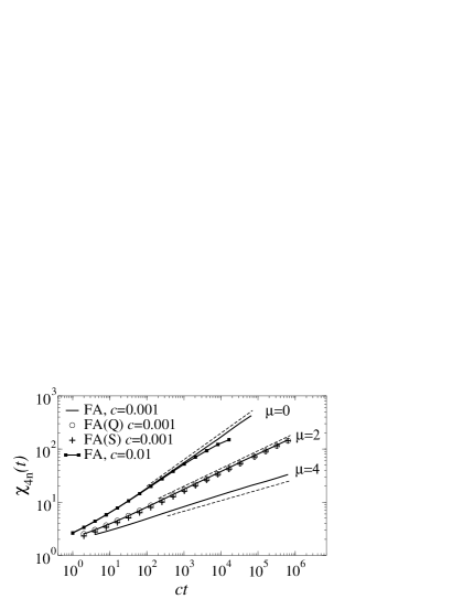
Figure 2: Subdiffusion in the FA and BBL models is apparent in the four point susceptibility. (Top) We show $\chi_{4\mathrm{n}}(t)$ in the BBL model at various $\mu$ and $\eta$. For the case $\mu=0$, we use a binary distribution of on-site densities $P_{\mathrm{s}}(\rho)\propto\alpha\delta(\rho)+\delta(2-\rho-0^{+})$, so that $\eta=\alpha(2+\alpha)/(1+\alpha)^{2}$; the small offset $0^{+}$ ensures that the facilitation constraint is well defined. The dashed lines show the power law predictions of (24), and simple diffusive scaling (23) for $\mu=0$. At large times, $\chi_{4\mathrm{n}}(t)$ saturates at a value of order $\eta^{-1}$: this is apparent in the data for $\mu=0$. The label (G) denotes data for the grand canonical variant of the BBL model. (Bottom) Bond-disordered FA model data with the same values of $\mu$, showing that this effective model captures the four point correlations of the BBL model. The labels (Q) and (S) denote data from the model with quenched bond disorder and fluctuating site disorder respectively; the different variants have very similar behaviour.

III.1 Effective barrier models for single excitations

Figure 2 is clear evidence that both BBL and disordered FA models have excitations that propagate subdiffusively at large $\mu$. Further, the dynamical exponents for all the models with $\mu>1$ seem to satisfy (24).

For the FA model with quenched bond disorder, this result is to be expected since the motion of independent random walkers in this kind of environment is well-understood BouchaudG90 and does indeed satisfy (24). However, it was argued in BBL05 that fluctuating disorder should lead to

$$z=\mu,\qquad\mu>2$$ (28)

and $z=2$ otherwise. This result is inconsistent with the data.

We are not aware of any analysis of fluctuating disorder that is slaved to the motion of the random walker. In this section, we give an argument that explains the applicability of (24) to the FA model with fluctuating disorder, and hence to the BBL model. While this is not a rigorous proof, the various stages of the argument have been verified by direct simulation.

To describe the motion of a single excitation in a disordered environment, we consider a simple barrier model BouchaudG90 . A single particle moves on a chain of sites, with independent random hop rates $\{r_{i}\}$ on the bonds, distributed according to $P_{r}(r)$. We consider both quenched and fluctuating disorder: if the disorder is fluctuating, then each random rate is redrawn from the distribution $P_{\mathrm{ann}}(r)$ when the bond is traversed by the random walker. We have verified by simulation that both variants of this model do indeed satisfy (24). We explain this result using an argument related to that of le Doussal, Monthus and Fisher DoussalMF99 . The effective dynamics scheme that we use for the barrier model with quenched disorder was described in Jack-duality-08 , where it was shown that the effective dynamics are a good description of the quenched barrier model, as long as the exponent $\mu$ is large. We give a brief description of the effective dynamics here, referring to Jack-duality-08 for details.

In DoussalMF99 , the authors proposed an effective dynamics for a random walker in a (quenched) one-dimensional energy landscape, made up of ‘barriers’ and ‘valleys’. At each stage of the effective dynamics, the smallest barrier in the system is removed, and the particle moves to the bottom of the valley that contains the origin. The time associated with this process is the inverse transmission rate of the barrier that was removed. For models in which the energy landscape has short-ranged correlations, this effective dynamics mimics the real dynamics of the random walker.

For the quenched barrier model, every site is at zero energy, and they are separated by barriers of varying heights. The effective dynamics involves successive removal of the smallest barriers. Thus, at a given stage of the dynamics, the remaining barriers divide the system into ‘effective traps’. As discussed in Jack-duality-08 , the barrier model requires a modification to the scheme of DoussalMF99 , in that the time at which barrier $i$ is removed depends both on the rate $r_{i}$ and on the widths of the effective traps to the left and right of barrier $i$. If the widths of these traps are $l_{1}$ and $l_{2}$, the time $\tau_{i}$ associated with barrier $i$ is determined by $\tau_{i}^{-1}=r_{i}(1/l_{1}+1/l_{2})$.

To arrive at the subdiffusive scaling of the quenched barrier model, we assume that, at time $t$, effective traps have a typical width $\ell(t)$. All barriers with $\tau_{i}<t$ have been removed; typically, these barriers have $r_{i}\gtrsim\ell(t)/t$ typical-foot . Thus, the density of remaining barriers is

$$\ell(t)^{-1}\simeq\int_{0}^{\ell(t)/t}\mathrm{d}r\,P_{r}(r)$$ (29)

which yields (for large $t$)

$$t\sim\ell(t)^{1+\mu}.$$ (30)

The mean square displacement of the diffusing excitation scales with $\ell(t)^{2}$, so we identify the dynamic exponent $z=1+\mu$, consistent with (24). Recall that the effective dynamics scheme applies only for large $\mu$, so we do not recover the diffusive result, $z=2$ for $\mu<1$.

We now apply this scheme to models with fluctuating disorder. The fluctuations in the disorder have two main effects. Firstly, once large barriers have been crossed, their rates are randomised. Thus, if multiple crossings of the same large barrier are important for the quenched model, we expect different behaviour for fluctuating disorder. However, a central assumption of the effective dynamics is that the time to travel a distance $\ell$ is dominated by the time required for the first crossing of the largest barrier between the initial and final sites Jack-duality-08 . Hence, multiple crossings of large barriers are ignored in the effective dynamics, which should therefore be consistent with fluctuating disorder. The second effect of fluctuating disorder is that barrier transmission rates are being randomised as the excitation moves around, so a barrier which previously had a large transmission rate may acquire a new rate that is very small. This new rate would then act as a high barrier and so have a strong effect on the resulting motion. As before, the time taken to move a distance $\ell$ will be given by the time taken to cross the largest barrier between initial and final states: this might be a barrier that was present initially, or one that appeared as the excitation moved through the system. The key point here is that the system is in a steady state, so the introduction of new barriers occurs with the same rate as the removal of barriers of the same size. Since barriers are removed only when they are crossed, barriers that appear in the system are typically of a size comparable with those that have already been crossed at least once. In the language of the effective dynamics, these barriers are ‘irrelevant’. For these reasons, the effective dynamics apply equally well to models with quenched and fluctuating disorder, and we expect the dynamical exponent $z=1+\mu$ for both cases.

Of course, the situation would be very different if the fluctuating disorder was annealed in a two-sided way, where every time an excitation moved to a new site one randomises the rates for both of the barriers adjacent to that site. This would produce a continuous-time random walk BouchaudG90 , with subdiffusion exponents as in Eq. (28).

To obtain the scaling of length and time scales in the FA and BBL models, we note that the equilibrium spacing between defects sets the dynamical correlation length $\xi$ (for these one-dimensional models). We define the persistence time $\tau_{\mathrm{p}}$ by $\langle p_{i}(\tau_{\mathrm{p}})\rangle=1/\mathrm{e}$, where $p_{i}(t)$ is the persistence function, defined above. As in the pure FA model, $\tau_{\mathrm{p}}$ scales with the time taken for an excitation to propagate a distance $\xi$, so we identify $\tau_{\mathrm{p}}\sim\Omega^{-1}\xi^{z}$, consistent with (27). To obtain the scaling of $\Omega$ with the excitation density $\eta$ or $c$, it is useful to rephrase the scaling argument associated with the effective dynamics. In the BBL model, Eq. (15) implies that the fraction of sites with rate $r_{i}<r$ scales as

$$n(r)\sim(r/\Omega_{0})^{1/\mu}$$ (31)

for small $r$. Thus, moving a distance $\ell$ typically requires the particle to cross a barrier whose transmission rate is $r_{i}\simeq\Omega_{0}\ell^{-\mu}$. The time taken to cross such a barrier is typically $\tau_{i}\sim\ell/r_{i}\sim\Omega_{0}^{-1}\ell^{1+\mu}$. This is consistent with (30), and it allows us to identify the coefficient $\Omega$ in (27) with $\Omega_{0}$ in (15). In the FA model, crossing a barrier with transmission rate $r_{i}$ typically requires a spin to flip from state $0$ to state $1$, and this process occurs with rate $e^{-\beta}\sim c$. Thus, moving a distance $\ell$ typically requires the crossing of a barrier with $r_{i}\simeq\ell^{-\mu}$, which takes a time $\tau_{i}\sim\ell/(r_{i}c)\sim c^{-1}\ell^{1+\mu}$. Thus, we identify the coefficient $\Omega$ in (27) with the inverse excitation density $c$. Overall, for $\mu>1$, we arrive at $\tau_{\mathrm{p}}\sim c^{-2-\mu}$ for the FA model, and $\tau_{\mathrm{p}}\sim[\ln(1/\eta)]^{-\mu}\eta^{-1-\mu}$ for the BBL model, where we used $\Omega_{0}\sim\gamma^{-\mu}\sim[\ln(1/\eta)]^{-\mu}$.

We conclude that the effective dynamics scheme presented here captures the propagation of mobility excitations in the BBL and disordered FA models on large length and time scales, even though the BBL model has non-trivial dynamical correlations in the densities $\rho_{i}$ which the coarse-grained FA model neglects. This analysis demonstrates that the scaling properties of the persistence time and the four-point susceptibility, as expressed in (23), (24) and (27), can be understood in terms of independently propagating (non-cooperative) excitations.

III.2 Long-time limit

So far, we have considered time scales up to the persistence time $\tau_{\mathrm{p}}$: excitations move distances smaller than their typical spacing, and can be treated independently. We now turn to much longer time scales. The assumption of independently propagating defects in one dimension leads to a persistence function consistent with the results of BBL05 :

$$p(t)\equiv\langle p_{i}(t)\rangle=\exp\left[-\frac{(\Omega t)^{1/z}}{\xi}\right]$$ (32)

for $t\gg 1$.

However, for times larger than $\tau_{\mathrm{p}}$, this prediction fails. For example, in the site-disordered FA model, the fraction of sites with rate $r_{i}<r$ is $n(r)=r^{1/\mu}$. At infinite temperature ($\beta=0,c=1/2$), the facilitation constraint in the FA model can be ignored (most sites are faciliated). In that case, the typical time taken to flip (for the first time) a site with initial rate $r_{i}$ is $\tau_{i}=1/r_{i}$. Thus, the persistence function decays as $\langle p_{i}(t)\rangle_{\beta=0}\simeq n(t^{-1})\simeq t^{-1/\mu}$. Lowering the temperature in the FA model only slows down the dynamics, so $\langle p_{i}(t)\rangle\gtrsim t^{-1/\mu}$ for all times and temperatures. Thus, (32) must break down at long times: we attribute this breakdown to the fact a single site with a small rate $r_{i}$ can block the motion of several excitations.

We now consider this long-time regime in more detail, and return to the effective dynamics picture, working with a finite density of excitations, $\eta$. If the density of relevant barriers is larger than the density of excitations, each effective trap typically contains at most one excitation, and excitations can be treated independently. However, when the spacing between relevant barriers becomes larger than the distance between excitations, one enters a different regime. To see this, note that the typical time scale associated with rearrangement of a ‘slow’ (relevant) site $i$ in the BBL model is generically $\tau_{i}=1/[r_{i}(\eta_{i-1}+\eta_{i+1})]$ where $\eta_{i-1}$ and $\eta_{i+1}$ are the excitation densities in the effective traps to left and right of site $i$. (Recall that $r_{i}$ is the rate with which the relevant site rearranges, given that there is an excitation adjacent to that site. Thus, the time taken to flip a relevant site depends on the density of excitations in the adjacent traps.)

In the short-time regime where there are many more effective traps than there are excitations, then we can write $\eta_{i}\simeq 1/l_{i}$ if trap $i$ contains an excitation, and $\eta_{i}=0$ otherwise (as above, $l_{i}$ is the width of effective trap $i$). Considering a site $i$ for which one of the adjacent traps contains an excitation, we arrive at the scaling relation $\tau_{i}\simeq l_{i}/r_{i}\simeq\ell/r_{i}$, as discussed above. However, if there are more excitations than effective traps, we expect the density in each trap to be close to its equilibrium value $\eta_{i}\simeq\eta_{i+1}\simeq\eta$. Thus, we expect $\tau_{i}\sim(2\eta r_{i})^{-1}$ for $\ell\eta\gg 1$. In both cases, for a given time $t$, we use $n(r)\simeq(r/\Omega)^{1/\mu}$ to evaluate the fraction of sites with $\tau_{i}<t$: the mean spacing between these “relevant” sites is $\ell(t)$. The result is

$$\ell(t)\sim\left\{\begin{array}[]{ll}(\Omega t)^{\frac{1}{1+\mu}},&\ell(t)\ll\xi\\ (\Omega t/\xi)^{1/\mu},&\ell(t)\gg\xi\end{array}\right.$$ (33)

where we have used $\xi\sim\eta^{-1}$. For long times, the exponent $\frac{1}{\mu}$ sets the time dependence of $\ell(t)$: this result applies for all $\mu>0$. In the short time regime, (33) is consistent with the analysis of the previous section, and with Eq. (27), as long as $\mu>1$. However, if $\mu<1$, the motion of excitations is diffusive: thus, in the short time regime, there is no distinction between relevant and irrelevant barriers. This means that if $\mu<1$, the spacing between relevant barriers, $\ell(t)$, is only well-defined in the long time limit, and the short-time scaling regime of (33) does not exist.

We observe that in the long time limit, $\ell(t)$ represents the mean spacing between isolated sites with small rates $r_{i}$, and these sites dominate the long-time limit of the persistence function. That is, in the long time scaling regime, (32) is replaced by

$$p(t)\simeq\ell(t)^{-1}\simeq(\Omega t/\xi)^{-1/\mu}.$$ (34)

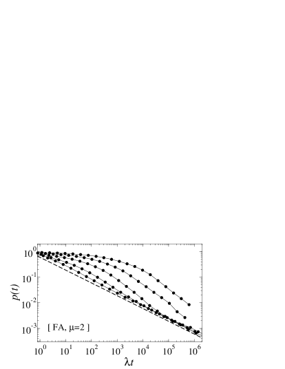
Figure 3: (Top) Persistence function, plotted against the scaling variable $\lambda t$ in the site-disordered FA model. We show data for that $c=0.5,0.27,0.12,0.047,0.018$ (decreasing from left to right, these are inverse temperatures $\beta=0,1,2,3,4$). As discussed in the text, the persistence time scales as $\tau_{\mathrm{p}}\sim c^{-2-\mu}\sim c^{-4}$, but we use the variable variable $\lambda t$ to verify the long time prediction of (35): the dashe lines shows a power law with exponent $\frac{1}{2}$. (Bottom) Persistence at infinite temperature and varying $\mu$. Again, dashed lines show power laws with exponents predicted by (35).

The crossover between the two scaling regimes occurs when $\ell(t)\simeq\xi\simeq\eta^{-1}$ or $c^{-1}$, respectively. This can be observed in the long-time behaviour of the persistence function in the site-disordered FA model. To obtain the long-time limit of this function more quantitatively, we decompose the persistence $p(t)=cp_{1}(t)+(1-c)p_{0}(t)$ into contributions from sites that were initially in states $1$ and $0$ [these two populations have weights $c$ and $(1-c)$ respectively]. Then, in the long time regime $\ell\gg\xi$, we have $\tau_{i}\simeq(2cr_{i})^{-1}$ for sites that were initially in state 1, given that each of the two facilitating neighbour sites contains a defect with probability $c$. For those sites initially in state 0, the spin flip rate is suppressed by $\mathrm{e}^{-\beta}$, leading to $\tau_{i}\simeq(2c\mathrm{e}^{-\beta}r_{i})^{-1}$. The persistence functions are then estimated as the density of sites with $\tau_{i}>t$, giving $p_{1}(t)=n(1/(2ct))$ and $p_{0}(t)=n(1/(2c\mathrm{e}^{-\beta}t))$, respectively. Using $n(r)=r^{1/\mu}$, we thus arrive at

$$p(t)\simeq(\lambda t)^{-1/\mu}\qquad\ell(t)\gg\xi\sim c^{-1}$$ (35)

with

$$\lambda=2c\mathrm{e}^{-\beta}[1+c(\mathrm{e}^{-\beta/\mu}-1)]^{-\mu}$$ (36)

In the limit of dilute excitations ($c\ll 1$) this reduces to $\lambda\sim c^{2}$. Identifying $p(t)$ with $\ell(t)^{-1}$, this result is consistent with (33), since we argued in Section III.1 that $\Omega\sim c$ for the FA model.

Results are shown in Fig. 3: at infinite temperature the power-law behaviour of the persistence is clear. At lower temperatures, the crossover to power-law behaviour occurs deep in the tails of the persistence [$p(t)\lesssim c$]. In the FA model, this long time regime can be demonstrated by simulations at high temperature, on relatively short time scales. However, in the BBL model, the equivalent of the high-temperature regime requires small $\gamma$, increasing the prefactor $\Omega_{0}$, and reducing the fraction of sites with small $r_{i}$. This means that very long simulations are required to access the long-time limit in the BBL model, and we do not show numerical data in this case. However, the simulations of the site-disordered FA model confirm the validity of the arguments of this section, which apply to both FA and BBL models. (To observe the long-time regime in the bond-disordered FA model, one would need to define and measure a persistence observable on bond $i$, associated with the rearrangement of density across that bond.)

IV Probe particles

It is a familiar feature of kinetically constrained models that propagation of probe particles is different from that of excitations JungGC04 ; BGC-Fick ; Chandler06 ; Kelsey08 . We now turn to probe particle motion in the BBL and disordered FA models.

IV.1 Probes in the BBL model

We introduce (non-interacting) probe particles to the BBL model as follows. A probe can move along a bond when density rearranges across that bond. If the bond connects sites $i$ and $i+1$, then after the rearrangement, the probe occupies site $i$ with probability $\rho_{i}/(\rho_{i}+\rho_{i+1})$. The joint stationary distribution for the probe position and the BBL densities is

$$P_{\mathrm{probe,stat}}(X,\{\rho_{i}\})\propto\rho_{i=X}\prod_{i}P_{\mathrm{s}}(\rho_{i}),$$ (37)

where $X$ is the position (site index) of the probe. Thus, the probability of finding a probe on site $i=X$ is is proportional to the local BBL density on that site, $\rho_{i=X}$. This is consistent with the probe representing a typical particle in the BBL model, before the coarse-graining into the densities $\rho_{i}$ is carried out. An alternative rule, which is more consistent with the effective FA model described below, is to assign a probe with equal probability to sites $i$ and $i+1$. As we discuss below, the excitation motion in these models sets bounds on the motion of the probes: we are primarily concerned with the situation in which these bounds are saturated, in which case details of the microscopic probe motion should be irrelevant. When the bounds are not saturated, the choice of dynamical rule does produce quantitative differences, although qualitative features are preserved.

IV.2 Probes in the FA model

We couple probe particles to the FA model using the method of JungGC04 . Probes can hop between pairs of adjacent sites only when both sites have $n=1$; they attempt these hops with unit rate. With these rules, the equilibrium distribution analogous to (37) is independent of $X$: that is, the distribution of the probe position decouples from the excitation variables $n_{i}$ and the rates $r_{i}$.

From the data presented above on the excitation dynamics of the site-disordered and bond-disordered FA models, one might expect that the two model variants also exhibit similar probe dynamics. However, this is not the case because barriers to excitation diffusion act differently on the probes. To see this, consider the site-disordered model, and suppose that site $i$ starts with $n_{i}=0$ and with a small rate $r_{i}$. The probe cannot cross this site until its excitation state changes to $n_{i}=1$. The rate for this is of order $cr_{i}$, and so the rate for a probe to cross this site also vanishes with $r_{i}$: high barriers for excitations (small $r_{i}$) are also high barriers for probes in the site-disordered FA model.

Now consider the bond-disordered FA model, focusing on a particular bond $i$, with a small rate $r_{i}$. The probe particle can cross this bond if $n_{i}=1$ and $n_{i+1}=1$: this state can occur on time scales much shorter than $(cr_{i})^{-1}$ if an excitation arriving from the right facilitates $n_{i+1}$ and another excitation arriving from the left facilitates $n_{i}$. This process sets a rate for crossing the slow bond that is independent of $r_{i}$. So the barriers for excitation diffusion have a much smaller effect on probe propagation in the bond-disordered model. (One way to avoid this behaviour would be to allow the probe to move along bond $i$ only when the rate for that bond is randomised, but we have not pursued this as we wanted to keep the probe dynamics similar to that used in JungGC04 .)

It is clear that in the original BBL model, the barriers for excitation diffusion do also act on probes. A high barrier here is a site with density $\rho_{i}\approx 2$. This can take part in a rearrangement only once a rearrangement of neighbouring sites has produced a low-density $\rho_{i-1}<2-\rho_{i}$ or $\rho_{i+1}<2-\rho_{i}$. The rate for these processes, and hence for probe diffusion across site $i$, vanishes as $\rho_{i}\to 2$. In summary, only the site-disordered FA model can provide an accurate representation of the BBL probe dynamics because it retains the effect of high barriers on the probes. We therefore do not consider the bond-disordered case in the following.

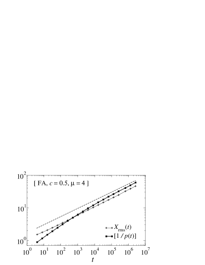
Figure 4: Comparison of root mean square probe displacement $X_{\mathrm{rms}}(t)=\langle X(t)^{2}\rangle^{1/2}$ with the inverse of the persistence function $1/p(t)$, for the site-disordered FA model. We show data at $\mu=3$ (top panel) and $\mu=4$ (bottom panel). We have offset the data at $c=0.25$ for clarity: the ordinate is $10t$ in that case. In the long-time limit, the persistence scales as $t^{-1/\mu}$ (this power law is illustrated with dashed lines). At long times the persistence sets a bound on the scaling of the mean square displacement, which appears to saturate for long times.

IV.3 Results for probe motion

In the BBL and site-disordered FA models, the preceding discussion illustrates that sites with small rate $r_{i}$ are able to block the propagation of probes. Taking the FA model for concreteness, the probe cannot pass any site for which $n_{i}=0$ for all times between $0$ and $t$. As discussed in Section III.2, the mean spacing between these sites scales as $t^{1/\mu}$ for large times $t$. This sets a limit on probe motion

$$\langle X(t)^{2}\rangle\lesssim\ell(t)^{2}\sim t^{2/\mu}$$ (38)

For $\mu<2$, this bound is irrelevant: the probes simply diffuse. However, for $\mu>2$, we expect this bound to be saturated at large times. At long times, we have $\ell(t)\sim p(t)^{-1}$, [recall (34)]. Thus, Fig. 4 demonstrates that the bound (38) does saturate at long times, although we note that the times required are quite large, even at infinite temperature ($c=1/2$). Physically, the length scale $\ell(t)$ represents the size of an effective trap: saturation of the bound requires that the probe particle explores the whole of the trap before the barriers delimiting the trap become irrelevant. The scaling arguments presented here do not allow us to estimate the time required to reach this regime. However, Eq. (38) shows that probe propagation must be asympotically subdiffusive for all $\mu>2$, and the data are consistent with saturation of this bound throughout this regime.

We emphasise that while Fig. 4 demonstrates that (38) holds on long time scales in the FA model, the scaling arguments presented here apply equally well to the BBL model, so asymptotic probe motion in that model must be subdiffusive for $\mu>2$.

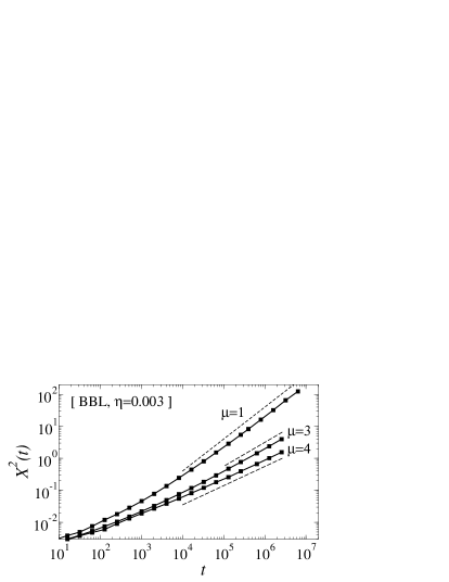
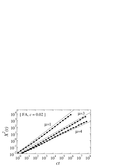
Figure 5: Mean-square probe displacements in the BBL and FA models, for times shorter than $\tau_{\mathrm{p}}$. (Top) BBL model. For $\mu>2$, the dashed lines show the predictions of (40); for $\mu=1$, we show a diffusive law $\langle X^{2}(t)\rangle\sim t$. (Bottom) Site-disordered FA model, with the same power-law predictions. In both cases, we expect a crossover at long times to the asymptotic scaling of (38).

We now turn to time scales shorter than $\tau_{\mathrm{p}}$, for which the length scale $\ell$ again sets a bound on probe motion. Following BGC-Fick , we decompose the probes into two populations: those that have moved at least once, and those which have not moved at all. We denote the fraction of probes that have moved at least once by $\pi(t)$. Confinement of probes by sites that are persistently unfaciliated again sets an upper bound on the displacement of probes:

$$\frac{\langle|X(t)|^{n}\rangle}{1-\pi(t)}\lesssim\ell(t)^{n}$$ (39)

where the left hand side is the $n$th moment of the distance moved by those probes that have moved at least once, and the scaling of $\ell(t)$ was given in (33). Again, saturation of this bound occurs when motion of the probe particle within the effective trap is fast enough that the the probe can delocalise within the trap before the barriers delimiting the trap become irrelevant. In the joint limit of large time and large $\mu$, the time scales associated with adjacent barriers become well-separated DoussalMF99 ; Jack-duality-08 , allowing equilibration to take place. Thus, for large $\mu$, we expect the bound of (39) to be saturated for times $t\gg 1$, even if $t\ll\tau_{\mathrm{p}}$.

Assuming saturation of the bound (39) and $t\ll\tau_{\mathrm{p}}$, the probe persistence scales as $1-\pi(t)\sim 1-\exp(-\ell(t)/\xi)\sim\ell(t)/\xi.$ (This is the same scaling as for the excitation persistence in (32).) Combining this with (33), we arrive at

$$\langle|X(t)|^{n}\rangle\sim\xi^{-1}(\Omega t)^{\frac{1+n}{1+\mu}},$$ (40)

Our simulations are restricted to finite time scales and values of $\mu$ that are not very large, so we are not able to investigate this bound in detail. However, the results shown in Fig. 5 are certainly consistent with the prediction of (40).

V Conclusion

To summarise our main results, we have established that probes and mobility excitations both propagate subdiffusively in the BBL model, and that this subdiffusive behaviour can be reproduced in a simple effective FA model. This observation allows us to analyse the subdiffusive motion, and to predict the dynamical exponents for both excitations and probes in the subdiffusive regime [Eqs. (24) and (38)]. A key part of the reasoning consists in showing that quenched and annealed disorder lead to qualitatively the same behaviour. This allowed us to deduce that correlation length and time scales are related in these models, by $\tau\sim\xi^{1+\mu}$. When $\mu$ is large, we conclude that the very broad distribution of rates in these models leads to a relaxation time that increases much more quickly than the associated length scales, on approaching the glass transition.

We also identify two kinds of subdiffusive motion in these models. On time scales $1\ll t\ll\tau_{\mathrm{p}}$, mobility excitations propagate independently and subdiffusively, according to

$$\langle X^{2}\rangle\simeq(\Omega t)^{\frac{2}{1+\mu}}$$ (41)

One has to remember though that this $\langle X^{2}\rangle^{1/2}$ does not define a lengthscale for probe motion, since it arises from an average over a dominant population of probes that have not yet moved, and a smaller population that has moved by $(\Omega t)^{1/(1+\mu)}$. For the same reason the exponent for the scaling of $\langle|X(t)|^{n}\rangle$ in Eq. (40) is not simply proportional to $n$. On time scales $t\gg\tau_{\mathrm{p}}$, excitations coagulate and branch, and it is not consistent to discuss motion of a single excitation. However, in this long-time regime, probe particles propagate subdiffusively, according to

$$\langle X^{2}\rangle\simeq(\Omega t/\xi)^{2/\mu}$$ (42)

The presence of different dynamical exponents for probes and excitations may seem surprising, but we emphasise that (41) and (42) apply in separate scaling regimes. (When the concentration of excitations is small, the persistence time $\tau_{\mathrm{p}}\gg 1$ separates two well-defined scaling regimes; of course $t$ is always taken to be large compared to unity.)

Conceptually, it is interesting to note that in the pure FA model at low temperature, relaxation is controlled by rare active sites (defects). In the disordered model, on the other hand, rare inactive regions (sites with small $r_{i}$) play at least as important a role.

Finally, our results for probe particles imply that the Stokes-Einstein relation DHReviews between relaxation time and probe diffusion constant, $D\tau\sim 1$, has broken down completely in these systems. In the pure FA model, $D\tau$ diverges at low temperatures JungGC04 . On the other hand, in the disordered model, the presence of sites (or barriers) with arbitrarily small rate $r_{i}$ means that the persistence decays as a power law for large times, while the motion of the probes is subdiffusive even in the long time limit. However, we can define an analogue of the Fickian length $\ell_{\mathrm{F}}=\langle X^{2}(\tau_{\mathrm{p}})\rangle^{1/2}$ which represents the distance travelled by a probe, through repeated encounters with a single excitation BGC-Fick . If the bound of (39) is saturated we arrive at $\ell_{\mathrm{F}}\simeq\ell(\tau_{\mathrm{p}})\simeq\xi$. For the site-disordered FA model, this leads to $\ell_{\mathrm{F}}\sim c^{-1}$, at least for large $\mu$; on the other hand, in the pure FA model, $\ell_{\mathrm{F}}\sim c^{-1/2}$. Physically, confinement of the excitation in an effective trap means that it facilitates any probes in that trap very many times, allowing the probe to delocalise thoughout the trap. In this way, the presence of large barriers to excitation diffusion in the BBL and disordered FA models strengthens the effects discussed in JungGC04 ; BGC-Fick , in which the square of the Fickian length represents the number of hops that a probe makes through multiple encounters with a single excitation.

- (1)
- (2) For a review, see F. Ritort and P. Sollich, Adv. Phys. 52, 219 (2003).
- (3) J. P. Garrahan and D. Chandler, Phys. Rev. Lett. 89, 035704 (2002).
- (4) Y.-J. Jung, J. P. Garrahan and D. Chandler, Phys. Rev. E 69, 061205 (2004).
- (5) L. Berthier, D. Chandler and J. P. Garrahan, Europhys. Lett. 69, 320 (2005).
- (6) E. Bertin, J.-P. Bouchaud and F. Lequeux, Phys. Rev. Lett. 95, 015702 (2005).
- (7) D. Chandler, J. P. Garrahan, R. L. Jack, L. Maibaum and A. C. Pan, Phys. Rev. E 74, 051501 (2006).
- (8) C. Toninelli, G. Biroli and D. S. Fisher, Phys. Rev. Lett. 96, 035702 (2006)
- (9) L. Berthier et al., J. Chem. Phys 126, 184504 (2007).
- (10) For reviews of the effects of dynamical heterogeneity and breakdown of the Stokes-Einstein relation, see: H. Sillescu, J. Non-Cryst. Solids 243, 81 (1999); M.D. Ediger, Annu. Rev. Phys. Chem. 51, 99 (2000). S.C. Glotzer, J. Non-Cryst. Solids, 274, 342 (2000); R. Richert, J. Phys. Condens. Matter 14, R703 (2002); H. C. Andersen, Proc. Natl. Acad. Sci. U. S. A. 102, 6686 (2005).
- (11) W. Kob and H. C. Andersen, Phys. Rev. E 48, 4364 (1993); C. Toninelli, G. Biroli and D. S. Fisher, J. Stat. Phys. 120, 167 (2005); C. Toninelli, G. Biroli and D. S. Fisher, Phys. Rev. Lett. 96, 035702 (2006).
- (12) J. Jäckle and A. Krönig, J. Phys.: Condens. Matter 6, 7633 (1994); A. C. Pan, J. P. Garrahan and D. Chandler, Phys. Rev. E 72, 041106 (2005).
- (13) G. H. Fredrickson and H. C. Andersen, Phys. Rev. Lett. 53, 1244 (1984).
- (14) S. Eisinger and J. Jäckle, J. Stat. Phys. 73, 643 (1993).
- (15) T. Odagaki and Y. Hiwatari, Phys. Rev. A 41, 929 (1990); C. Monthus and J.-P. Bouchaud, J. Phys. A 29, 3873 (1996).
- (16) X. H. Qiu and M. D. Ediger, J. Phys. Chem. B 107, 469 (2003).
- (17) C. Dalle-Ferrier et al., Phys. Rev. E 76, 041510 (2007).
- (18) S. Whitelam, L. Berthier and J. P. Garrahan, Phys. Rev. Lett. 92, 185705 (2004);
- (19) S. Franz, C. Donati, G. Parisi, and S. C. Glotzer, Philos. Mag. B 79, 1827 (1999).
- (20) L. Berthier, Phys. Rev. E 69, 020201 (2004).
- (21) C. Toninelli, M. Wyart, L. Berthier, G. Biroli, and J.-P. Bouchaud, Phys. Rev. E 71, 041505 (2005).
- (22) R. L. Jack, P. Mayer, and P. Sollich, J. Stat. Mech. (2006), P03006.
- (23) See, for example, A. Widmer-Cooper and P. Harrowell, Phys. Rev. Lett. 93, 135701 (2004); A. Widmer-Cooper and P. Harrowell, J. Chem. Phys, 126 154503 (2007).
- (24) J.-P. Bouchaud and A. Georges, Phys. Rep. 195, 127 (1990)
- (25) R. L. Jack, L. Berthier and J. P. Garrahan, Phys. Rev. E 72, 016103 (2005).
- (26) P. le Doussal, C. Monthus and D. S. Fisher, Phys. Rev. E 59, 4795 (1999).
- (27) R. L. Jack and P. Sollich, J. Phys. A 41, 324001 (2008).
- (28) R. L. Jack, D. Kelsey, J. P. Garrahan and D. Chandler, Phys. Rev. E 78, 011506 (2008).
- (29) As discussed in Jack-duality-08 , these arguments based on a typical length scales are valid since the distribution of trap widths is much narrower than the distribution of time scales , so fluctuations in can be neglected.