A Simple Model for Solar Isorotational Contours

Abstract

The solar convective zone, or SCZ, is nearly adiabatic and marginally convectively unstable. But the SCZ is also in a state of differential rotation, and its dynamical stability properties are those of a weakly magnetized gas. This renders it far more prone to rapidly growing rotational baroclinic instabilities than a hydrodynamical system would be. These instabilities should be treated on the same footing as convective instabilites. If isentropic and isorotational surfaces coincide in the SCZ, the gas is marginally (un)stable to both convective and rotational disturbances. This is a plausible resolution for the instabilities associated with these more general rotating convective systems. This motivates an analysis of the thermal wind equation in which isentropes and isorotational surfaces are identical. The characteristics of this partial differential equation correspond to isorotation contours, and their form may be deduced even without precise knowledge of how the entropy and rotation are functionally related. Although the exact solution of the global SCZ problem in principle requires this knowledge, even the simplest models produce striking results in broad agreement with helioseismology data. This includes horizontal (i.e. quasi-spherical) isorotational contours at the poles, axial contours at the equator, and approximately radial contours at midlatitudes. The theory does not apply directly to the tachocline, where a simple thermal wind balance is not expected to be valid. The work presented here is subject to tests of self-consistency, among them the prediction that there should be good agreement between isentropes and isorotational contours in sufficiently well-resolved large scale numerical MHD simulations.

1 Introduction

The problem of differential rotation in the solar convective zone (SCZ) has vexed theorists for many years. At the simplest level, one is faced with the fact that the only region of the sun characterized by significant turbulence is also the only region showing any significant differential rotation. This is a cogent reminder of the hazards of modeling a rotating, turbulent gas by an effective viscosity parameter. The SCZ is far too complex to yield to such an approach. Indeed, large scale numerical simulations have been in place for many years, trying to elicit the rotation profile of the sun’s outer layers (Brummell, Cattaneo, & Toomre 1995; Thompson et al. 2003). While these studies are now at a stage where they can begin to make contact with the observational data, they have not yet been able to reproduce the salient features of the observed solar rotation profile. This is especially true for the isorotational contours (hereafter “isotachs”), which tend to be cylindrical in simulations, but are decidedly noncylindrical in the sun.

In this paper, we examine an effect that could be important for understanding the SCZ rotation profile, but has not been sufficiently emphasized in previous investigations: the extreme sensitivity of ionized differentially rotating gas to the presence of even very weak magnetic fields of arbitrary geometry (Balbus & Hawley 1994, Ogilvie 2007). Far from behaving as a passive vector field, a weak magnetic field triggers rapidly growing unstable local modes in rotating systems that would be hydrodynamically unstable. The field endows the gas with degrees of freedom that have no hydrodynamical counterpart. The classical manifestation of this behavior takes the form of what is known as the magnetorotational instability (MRI), widely regarded as the process responsible for turbulence and enhanced transport in accretion disks (Balbus & Hawley 1991, 1998). But destabilization by a weak magnetic field is a process that extends beyond the domain of rotationally supported disks. Such fields are agents of dynamical destabilization in baroclinic and convective flows as well (Balbus 1995), with potentially interesting applications to the SCZ.

It is essential to understand two key counterintuitive points at the outset. The first is that destabilization by a magnetic field can occur even when the field plays essentially no role in the dynamical equilibrium: a weakly magnetized gas does not behave “almost hydrodynamically” with respect to its stability properties. The second is that the destabilization is independent of the field strength and field geometry. In MRI simulations, the disruption remains vigorous and self-sustaining even in highly convoluted turbulent flow. This is what makes MHD processes potentially so important for understanding rotating, stratified flows.

It is the emphasis on these points that sets the present approach apart from earlier work that also addressed the stability of rotating, stratified, magnetized flows (e.g. Acheson 1983, Ogden & Fearn 1995). In these earlier studies, the focus is upon toroidal fields, nonaxisymmetric disturbances, and instability driven directly by the magnetic field. By contrast, what is crucial here are poloidal fields and axisymmetric disturbances. Moreover, while the instability of interest relies on the presence of a magnetic field, the (nonconvective) seat of free energy is the differential rotation, not the field itself. The role of the field is to provide the critical degrees of freedom to the fluid required to tap into the (destabilizing) differential rotation.

We shall begin our presentation, however, not with magnetic fields, but with a theoretical observation that may be taken at a purely phenomenological level, independently of deeper MHD considerations. This is the remarkable agreement with the overall pattern of solar isorotation contours produced by a simple calculation in which a dominant thermal wind balance from the vorticity equation is combined with the assumption that entropy and angular velocity gradients are counteraligned. Whatever the cause of the counteralignement may be, the analysis on its own is highly suggestive. (A connection between entropy and angular velocity gradients has in fact been advocated on purely hydrodynamical grounds [Miesch, Brun, & Toomre 2006].) This material is presented in §2. In §3, we discuss in some detail the case for an MHD coupling between angular velocity and entropy gradients. The final section is a critical discussion of unresolved issues provoked by this work, and a summary.

2 Solving the thermal wind equation

2.1 Review

Let $(R,\phi,z)$ be a standard cylindrical coordinate system, and $(r,\theta,\phi)$ a standard spherical coordinate system. Unit vectors are denoted $e_{R}$, $e_{\theta}$, etc. The angular velocity $\Omega$ is assumed to be independent of $\phi$, but otherwise general. Our notation for the fluid variables is likewise standard: $v$ is the velocity, $P$ is the gas pressure, $\rho$ is the mass density, and $B$ is the magnetic field.

We adopt a fiducial value of $2.5\times 10^{-6}$ rad s^-1 for the angular velocity $\Omega$ in the SCZ, corresponding to rotation velocities between 1 and 2 km s^-1. This is well in excess of the $\sim 30$ m s^-1 expected of convective velocities, but such a direct comparison is not necessarily the most relevant one. A more telling comparison is between the squared Brunt-Väisälä frequency

$$\left|N^{2}\right|=\left|-{1\over\rho\gamma}{\partial P\over\partial r}{\partial\ln P\rho^{-\gamma}\over\partial r}\right|\sim 3.8\times 10^{-13}\ {\rm s}^{-2}$$ (1)

(we have adopted a value of $10^{-6}$ for $\partial\ln P\rho^{-\gamma}/\partial\ln r$ [Schwarzschild 1958]) and the rotational parameter

$${d\Omega^{2}\over d\ln R}\sim 1.8\times 10^{-12}\ {\rm s}^{-2}.$$ (2)

This is evidently about 5 times as large as $N^{2}$. (Whether $R$ or $z$ is used in the angular velocity gradient is not critical at midlatitudes.) Taking this estimate at face value, the rotational parameter is significantly larger than $N^{2}$. The significance of this will shortly become apparent.

Let us first consider systems whose equilibrium velocity is differential rotation, $\mbox{\boldmath{$v$}}=R\Omega(R,z)\mbox{\boldmath{$e_{\phi}$}}$. The thermal wind equation follows directly from the time-steady form of the vorticity equation,

$$R{\partial\Omega^{2}\over\partial z}={1\over\rho^{2}}\left(\mbox{\boldmath{$\nabla$}}P\mbox{\boldmath{$\times$}}\mbox{\boldmath{$\nabla$}}\rho\right)\mbox{\boldmath{$\cdot$}}\mbox{\boldmath{$e_{\phi}$}}.$$ (3)

Expressing the right side in $r,\theta,\phi$ spherical coordinates:

$$R{\partial\Omega^{2}\over\partial z}={1\over r\rho^{2}}\left({\partial\rho\over\partial\theta}{\partial P\over\partial r}-{\partial\rho\over\partial r}{\partial P\over\partial\theta}\right).$$ (4)

Now, rewrite this in terms of the entropy gradients:

$$R{\partial\Omega^{2}\over\partial z}={1\over C_{P}\rho r}\left({\partial P\over\partial\theta}{\partial S\over\partial r}-{\partial P\over\partial r}{\partial S\over\partial\theta}\right),$$ (5)

where $S$ is the specific entropy,

$$S={k\over\gamma-1}\ln P\rho^{-\gamma}+{\rm constant},$$ (6)

$k$ is the Boltzmann constant, and $C_{P}$ is the constant pressure specific heat,

$$C_{P}=\left(\gamma\over\gamma-1\right)k$$ (7)

In the SCZ, the $r$ gradient of $P$ clearly dominates over the $\theta$ gradient, whereas the $r$ gradient of $S$ is unlikely to greatly exceed the $\theta$ gradient. (In fact, we shall presently argue just the opposite.) We may then conclude that

$$R{\partial\Omega^{2}\over\partial z}={g\over\ C_{P}r}{\partial S\over\partial\theta}={g\over\gamma r}{\partial(\ln P\rho^{-\gamma})\over\partial\theta}$$ (8)

where $g=-(1/\rho){\partial P/\partial r}$ is the gravitational field in hydrostatic equilibrium, ignoring the small effects of rotation. Significant latitudinal entropy gradients are required to avoid cylindrical isotachs.

Equation (8) is known as the thermal wind equation (Kitchatinov & Rüdiger 1995, Thompson et al. 2003). This equation holds in our MHD analysis, because we explicitly assume that the magnetic fields are sufficiently weak in the equilibrium state that they do not affect the large scale rotation profile. (For a 10 G field and a density of $0.05$ g cm^-3, the Alfvén velocity is 13 cm per second.) In full spherical coordinates, the thermal wind equation is

$$\left(\cos\theta{\partial\Omega^{2}\over\partial r}-{\sin\theta\over r}{\partial\Omega^{2}\over\partial\theta}\right)={g\over C_{P}r^{2}\sin\theta}{\partial S\over\partial\theta}$$ (9)

Even before a detailed solution is developed, a simple scaling argument reveals something of interest here. The $r$ gradient of $S$ is generally determined by the need to transport the solar luminosity by thermal convection (Schwarzschild 1958, Clayton 1983). On the other hand, the $\theta$ gradient is, from equation (8), linked directly to differential rotation. If the fiducial numbers (1) and (2) are reasonably accurate, at midlatitudes equation (8) implies that the $\theta$ gradient of $S$ will significantly exceed the $r$ gradient. The point of interest here is that this anisotropic feature is directly seen in the $\Omega$ gradient deduced from the helioseismology data. This suggests that there is a deeper dynamical coupling present between $S$ and $\Omega$, beyond just the general trend that one goes up as the other goes down. We will develop this idea more fully in the next two sections.

2.2 Analysis

The thermal wind equation is a familiar tool to practitioners of solar rotation theory. The gross features of the sun’s angular velocity profile ($\Omega$ decreasing polewards from the equator) can be understood relatively simply with the aid of this equation and some reasonable assumptions of the efficiency of convection in the presence of Coriolis forces (Thompson et al. 2003). The idea is that convection in the equatorial direction is impeded by Coriolis forces, resulting in a more efficient transport of heat along the rotation axis. The poles are then regions of higher specific entropy compared with the equatorial zone, and the resulting $\theta$ gradient in $S$ drives axial gradients in $\Omega$.

This is a well-motivated and physically plausible scenario. It seems natural therefore, to search for explicit model solutions to the thermal wind equation incorporating this idea. Moving upward from the equator, we expect the angular velocity to decrease as the entropy increases. Clearly the gradients of these quantities are in broadly opposite senses. But the final paragraph of §2.1 suggests that “counteraligned” may be a better description then “broadly opposite.” This raises the question of what the solutions to equation (9) would look like if the two gradients were in fact precisely oppositely aligned.

Following the notion that isentropic and isorotational surfaces coincide, we assume that $S=S(\Omega^{2})$. ($S$ should not change if $\Omega$ changes sign, hence the dependence on $\Omega^{2}$.) Equation (9) then becomes

$${\partial\Omega^{2}\over\partial r}-\left({gS^{\prime}\over C_{P}r^{2}\sin\theta\,\cos\theta}+{\tan\theta\over r}\right){\partial\Omega^{2}\over\partial\theta}=0,$$ (10)

where $S^{\prime}\equiv dS/d\Omega^{2}$. The solution of equation (10) is that $\Omega^{2}$ is constant along the characteristic

$${d\theta\over dr}=-{\tan\theta\over r}-{gS^{\prime}\over C_{P}r^{2}\sin\theta\ \cos\theta}$$ (11)

But if $\Omega^{2}$ is constant along this characteristic, then so must be $S^{\prime}$. This is therefore a self-contained, ordinary differential equation for $\theta$ as a function of $r$, precisely the isorotational contours that we seek. To solve equation (11), let $y=\sin\theta$. Then, our differential equation simplifies to

$${dy^{2}\over dr}+{2y^{2}\over r}=-{2gS^{\prime}\over C_{P}r^{2}}$$ (12)

Multiplying by $r^{2}$ and regrouping,

$${d(r^{2}y^{2})\over dr}=-{2gS^{\prime}\over C_{P}}=-{2GM_{\odot}S^{\prime}\over C_{P}r^{2}}$$ (13)

where $G$ is Newton’s constant and $M_{\odot}$ is a solar mass. (We have ignored the local self-gravity of the SCZ.) Since $S^{\prime}$ is a constant along the characteristic, this integrates immediately to

$$r^{2}\sin^{2}\theta=R^{2}=A-{B\over r}$$ (14)

where $A$ is a constant of integration and

$$B=-{2GM_{\odot}S^{\prime}\over C_{P}}.$$ (15)

We have inserted a minus sign since $S$ will generally be a decreasing function of $\Omega^{2}$. Indeed, as will become very clear, the characteristics make no sense if $S^{\prime}$ is positive, but a very great deal of sense if it is negative. In this model, the solar isotachs are given by a remarkably simple formula.

To estimate the magnitude of $B$, note that it may be written

$${B\over r_{\odot}^{3}}=\left(2GM_{\odot}/r_{\odot}\over\gamma r_{\odot}^{2}\Omega^{2}\right)\left(-{d\ln P\rho^{-\gamma}\over d\ln r}\right)\left({d\ln r\over d\ln\Omega^{2}}\right)$$ (16)

The first factor is large, of order $10^{5}$. The second, we have already estimated at $10^{-6}$. The helioseismology data suggest that the third factor ranges between 1 and 10, and is larger near the equator. Crudely speaking, we expect $B/r_{\odot}^{3}$ to be of order unity or less. There should not be a large difference in scale between $A/r_{\odot}^{2}$ and $B/r_{\odot}^{3}$.

2.3 Alternative isotach solution

By way of comparison, consider the solution of the thermal wind equation that would obtain were the angular momentum counteraligned with the entropy, rather than the angular velocity. (In hydrodynamic baroclinic turbulence, one might expect the coupling to be of this nature since entropy and angular momentum tend to be retained by a displaced fluid element.) Then $S=S(l^{2})$, where $l=R^{2}\Omega$ is the specific angular momentum. We denote $dS/dl^{2}$ by $S_{l^{2}}$. Our analysis proceeds along lines identical to §2.2, and $l^{2}$ satisfies the PDE

$${\partial l^{2}\over\partial r}-\tan\theta\left({1\over r}+{gr^{2}\sin^{2}\theta S_{l^{2}}\over C_{P}}\right){\partial l^{2}\over\partial\theta}=0.$$ (17)

The contours of constant $l^{2}$ are found to be of the form

$${1\over R^{2}}={1\over r^{2}\sin^{2}\theta}=A_{l}+{B_{l}\over r}$$ (18)

where $A_{l}$ is an integration constant, and now

$$B_{l}=-{2GM_{\odot}S_{l^{2}}\over C_{P}}$$ (19)

Note that $r_{\odot}B_{l}$ is a dimensionless constant of order unity. We will use this solution as a point of comparison in the next section.

2.4 An explicit solution

Let us turn to the data to see how our solutions fare, beginning with our first, $\Omega$ based solution. As an illustrative example, consider the reduced problem in which $S^{\prime}$ is constant, not just along a particular characteristic, but everywhere. Then $B$ is also everywhere constant. If $\Omega$ is now specified on some particular radial shell as a function of $\theta$, we may write down the solution everywhere. For this purpose, it is easiest to choose the solar surface radius $r=r_{\odot}$.

Let the angular velocity at $r=r_{\odot}$ be $\Omega_{\odot}(\cos^{2}\theta_{0})$. We use the fit of Ulrich et al. (1988):

$$\Omega_{\odot}(\cos^{2}\theta_{0})=2\pi\left(451.5-65.3\cos^{2}\theta_{0}-66.7\cos^{4}\theta_{0}\right)\ {\rm nHz.}$$ (20)

Note that $\theta_{0}$ carries a subscript to indicate that it is the particular value of $\theta$ along each trajectory characteristic (14) that intersects the surface shell $r=r_{\odot}$. Equation (14) becomes

$$r^{2}\sin^{2}\theta=r_{\odot}^{2}\sin^{2}\theta_{0}+B\left({1\over r_{\odot}}-{1\over r}\right),$$ (21)

or

$$\cos^{2}\theta_{0}=1-x^{2}+\left(B\over r_{\odot}^{3}\right)\left(1-{1\over\varpi}\right)$$ (22)

where

$$\varpi=r/r_{\odot},\qquad x^{2}=\varpi^{2}\sin^{2}\theta.$$ (23)

(Equations (21) and (22) are also valid if $B$ is a function of $\cos\theta_{0}$.) Substituting equation (22) for $\cos^{2}\theta_{0}$ into equation (20) then generates the solution everywhere in the shell.

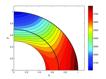
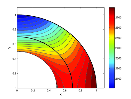
Figure 1: Contour plot of $\Omega(r,\theta)$ in solar interior, using surface fit of Ulrich et al. (1988). SCZ boundaries marked in white. Calculation based on eqs. [20] and characteristic equations of isorotational contours, [22]. $B/r_{\odot}^{3}=0.5\,{\rm(left)},\,0.6\,{\rm(right)}$.

The result of this procedure is shown in figure (1) for the cases $B/r_{\odot}^{3}=0.5,0.6$. The detailed fit of the contours to the actual data is not perfect—there is no tachocline in these simple models, and the true high latitude isotachs show stronger curvature, following spherical shells, before turning upward. But the overall trend of the isotachs being predominantly quasi-spherical at high latitudes, increasingly radial at midlatitudes, and axial at small latitudes is unmistakable. Moreover, fitting our solution to the observed surface data, while convenient, is unlikely to show off its best form: thermal wind balance probably breaks down near the solar surface (Thompson et al. 2003). Given the simplicity of our direct approach, the qualitative agreement is both striking and encouraging.

The iso-angular-momentum contours of equation (18) can also be used to construct an explicit solution. In this case, the surface angular momentum $l$ fit is

$$l(\cos^{2}\theta_{0})=2\pi r_{\odot}^{2}\sin^{2}\theta_{0}\left(451.5-65.3\cos^{2}\theta_{0}-66.7\cos^{4}\theta_{0}\right).$$ (24)

Instead of equation (22), we have

$$\cos\theta_{0}^{2}=1-\sin^{2}\theta_{0}=1-\left[{1\over x^{2}}+r_{\odot}B_{l}\left(1-{1\over\varpi}\right)\right]^{-1}$$ (25)

Substitution of (25) into (24) generates the full solution for the specific angular momentum $l(r,\theta)$, and the angular velocity solution follows immediately from

$$\Omega(\cos^{2}\theta_{0})=(2\pi/x^{2})\sin^{2}\theta_{0}\left(451.5-65.3\cos^{2}\theta_{0}-66.7\cos^{4}\theta_{0}\right)$$ (26)

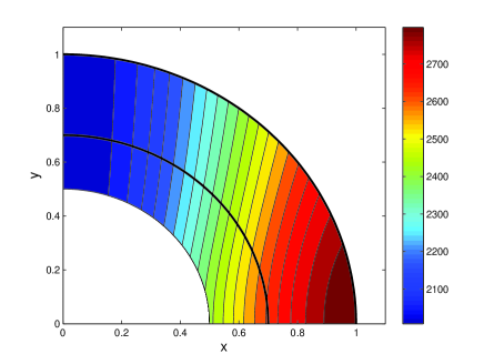
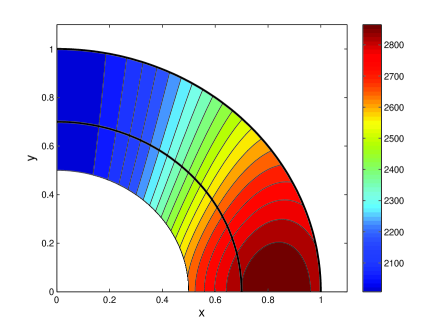
Figure 2: Contour plot of $\Omega(r,\theta)$ in solar interior, based on counter aligned entropy and angular momentum gradients, using surface fit of Ulrich et al. (1988). SCZ boundaries marked in white. Calculation based on eq. [26] and characteristic equation of iso-angular-momentum contours, [24]. $r_{\odot}B_{l^{2}}=0.2\,{\rm(left)},\,0.5\,{\rm(right)}$.

In figure 2, we show two representative diagrams of the isorotational contours taken from this alternative angular momentum based approach. In general the contours are too cylindrical, to some extent exhibiting the same syndrome often seen in numerical SCZ simulations. The contrast between figures 1 and 2 is very apparent. There seems to be a real linkage between $S$ and $\Omega$, and it matters very much that the coupling is between $S$ and $\Omega$, not $S$ and $l$. It is possible that the refractory nature of the cylindrical contours of the simulations is due to an $S-l$ coupling that remains too strong, as noted in in §2.3. While it is possible that this may be cured by a more highly resolved treatment of the turbulent fluid, it is also possible that magnetic fields may be playing a non-negligible role, enforcing an $S-\Omega$ coupling by field line tethering of the fluid elements. We pursue this possibility in §3.

In the remainder of the paper, we focus exclusively on our original $S-\Omega$ solution.

2.5 Tightening the contours

By allowing the $B$ parameter to vary from one isotach to another, the isorotational contours we have found can become more tightly spaced near the poles. In this sense, our solutions admit, but do not demand, something reminscent of tachoclinic structure. Equation (14) may be written

$$r={B/A\over 1-(R^{2}/A)}$$ (27)

If the variation of $\Omega$ leads to a nearly constant ratio for $B/A$ close to the outer radius of the radiative zone $r_{rad}$, but very different $A$ values, tachoclinic structure results. In the polar regions near the axis of rotation, the contours would all converge to $r_{rad}$, while corresponding to very different $\Omega$ values. This would look very much like a tachocline.

Does this make physical sense? Equation (21) implies $A=r_{\odot}^{2}\sin^{2}\theta_{0}+B/r_{\odot}$, or

$${B\over A}={r_{\odot}\over 1+(r_{\odot}^{3}\sin^{2}\theta_{0}/B)},$$ (28)

assuming that the data are initially specified on $r=r_{\odot}$. Hence, $B\propto\sin^{2}\theta_{0}$ would produce tachoclinic structure.

Physically , this would mean that $B\propto dS/d\Omega^{2}$ is small and negative near the pole, and that the entropy decreases toward the equator as $\Omega$ increases. In the vicinity of the equator the entropy drops sharply. This is not unreasonable behavior: near the pole, unencumbered by Coriolis deviations, convection is most effective, whereas at the equator, the opposite is true. At the same time, the observations suggest that $\Omega$ is changing rapidly near the pole, and only slowly at the equator. This is consistent with our simple picture.

We return to equation (22) and replace $B/r_{\odot}^{3}$ by

$$B/r_{\odot}^{3}=\eta_{1}+\eta_{2}\sin^{2}\theta_{0}.$$ (29)

Mathematically, this corresponds to the first two terms in a Taylor series expansion of $S^{\prime}$ as a function of $\sin^{2}\theta_{0}$ (or equivalently $\cos^{2}\theta_{0}$). By varying $\eta_{1}$ and $\eta_{2}$ we can go between a singular tachocline $\eta_{1}=0$ and the previous case $\eta_{2}=0$. Substituting (29) in (22) and solving for $\cos^{2}\theta_{0}$ gives

$$\cos^{2}\theta_{0}=1-{\varpi x^{2}-\eta_{1}(\varpi-1)\over\varpi+\eta_{2}(\varpi-1)}.$$ (30)

Using equation (30) in (20) now produces the interior structure $\Omega(r,\theta)$.

With two parameters available, one can of course produce somewhat better fits to the rotation profile. In practice, the improvement over §2.4 is noticeable, but not dramatic. In figure 3, we show on the left the isotachs for $\eta_{1}=0.3$, $\eta_{2}=0.2$. This gives a very respectable fit to the data away from the tachocline, $r\geq 0.75r_{\odot}$, say. If we wish to include an explicit tachocline in our modeling, our earlier considerations suggest that we should restrict ourselves to small values of $\eta_{1}=0$. On the right side of figure 3, the interesting case of $\eta=0.12$ and $\eta_{2}=0.8$ is presented. A striking “tachocline” structure appears, though formally it lies just beneath the SCZ. The solar midlatitude radial contours and equatorial cylinders regions are, however, rather well-represented. Note as well the gentle nonmonotonic behavior of $\Omega(R)$ near the equator, a feature seen in the helioseismology data. Increasing the value of $eta_{2}$ to bring the tachocline to larger radii (while keeping the surface layers fixed) appears to cause too much global distortion, though an exhaustive parameter search has not been performed.

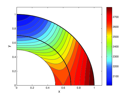
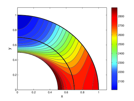
Figure 3: As in figure 1, but calculation now based on equations [20] and [30] with $\eta_{1}=0.3$, $\eta_{2}=0.2$ (left), and $\eta_{1}=0.12$, $\eta_{2}=0.8$ (right). The two-parameter fit on the left is a slight improvement over the earlier single parameter models. The fit on the right is striking in its overall resemblance to the SCZ, though the “tachocline” formally lies below the convective zone lower boundary. Equatorial and midlatitude contours are well-represented.

At this stage, these results are suggestive, but not more than that. It seems likely that more complex choices for $S^{\prime}(\Omega^{2})$ could improve the contour fits, but the agreement is impressive even in the simplest models. A truly compelling explanation of the tachocline will involve more than just the thermal wind equation and the outer convective zone layers. The solar tachocline arises from the complex coupling of the rigidly rotating radiative core and the overlying strongly shearing convective zone, not the demands of the surface rotation and vorticity conservation, and very different dynamical processes are likely to be involved. Our simple, prescription valid above the tachocline ($r\mathrel{\hbox to0.0pt{\lower 2.15277pt\hbox{$\mathchar 536\relax$}\hss}\raise 1.72218pt\hbox{$>$}}0.75r_{\odot}$) may represent a sort of outer SCZ solution that asymptotically matches onto an inner solution in which tachocline dynamics become locally dominant.

2.6 Generic features of isotachs

The isotachs we have found have a very distinctive “viking helmet” structure. This unusual feature is also characteristic of solar isorotation contours, and worth examining in isolation.

To understand the general structure of the isotachs, rewrite eqation (27) as

$${r\over r_{\odot}}={B/Ar_{\odot}\over 1-(r_{\odot}^{2}/A)(R^{2}/r_{\odot}^{2})}={\alpha\over 1-\beta R^{2}/r_{\odot}^{2}}$$ (31)

which defines our two parameters $\alpha$ and $\beta$,

$$\alpha=B/r_{\odot}A,\qquad\beta=r_{\odot}^{2}/A$$ (32)

We now transform to Cartesian coordinates in a meridional plane,

$$y=(r/r_{\odot})\cos\theta,\quad x=(r/r_{\odot})\sin\theta.$$ (33)

The Cartesian contour structure is slightly easier to visualize:

$$y=\left[{\alpha^{2}\over(1-\beta x^{2})^{2}}-x^{2}\right]^{1/2}$$ (34)

We must of course view equation (34) through the convective zone slot $0.7<\sqrt{x^{2}+y^{2}}<1$. There are three types of contours. The first is a typical polar contour, emerging perpendicular to the axis before bending upward, seen at high latitudes in figure 1. The second class, visible at midlatitudes in figure 1, is hidden in the radiative zone at small $x$, and does not emerge into the SCZ until the contour is well separated from the axis, at which point the isotach has a quasi-radial character. The third contour class is deeply buried, running along a very small radius in the core (not seen), completely disappearing in the bulk of the sun ($y$ is imaginary). It then makes a sudden leap upward into the equatorial region of the SCZ, where it appears nearly axial. These are the low latitude regions of figure 1, corresponding physically to Taylor columns of constant rotation on cylinders. Equation (34) thus displays the three key traits one associates with isotachs: horizontal near the poles, radial at midlatitudes, and cylindrical near the equator.

3 Axisymmetric modes in a rotating, baroclinic, weakly magnetized gas

3.1 Preliminaries

The starting point of the analysis of §2 was that the dominant balance of the vorticity equation is given by the thermal wind relation. We adopted a phenomenological connection between $S$ and $\Omega$ that succeded in reproducing the observed general behavior of the solar isorotational contours. In this section we examine a possible reason for this coupling. We suggest that the underlying cause of the $S-\Omega$ coupling is to be found in the general dynamical stability properties of a magnetobaroclinic fluid.

We have already noted that in accretion disk applications, the combination of magnetic fields and differential rotation is extremely destabilizing, even if the field is very weak and not particularly well-ordered. This is a consequence of the MRI. The analysis presented here is an extension of the accretion disk problem, but a highly significant extension: we consider the most general dynamical axisymmetric response to a weakly magnetized baroclinic system. To avoid possible confusion, we will reserve the term “MRI” to apply only to the magnetic destabilization process in rotation-dominated disks. The topic of this section is the “magnetobaroclinic instability.”

The system we analyze is a proxy that shares important features with the sun. It consists of a body of self-gravitating gas that has arbitrary axisymmetric angular velocity and entropy profiles. Instability in the form of turbulent thermal convection is treated on the same footing as rotational instability. Both the thermal and rotational profiles can in principle be altered by turbulent fluxes arising from magnetobaroclinic instability, since neither profile is fixed by the requirements of hydrostatic equilibrium. This differs from the behavior of an accretion disk, whose rotational profile, generally Keplerian, is not at liberty to change.

It is an elementary fact that a convectively unstable stratified gas tends to alter its thermal gradient to a nearly adiabatic configuration, thereby regulating the linear instability itself. What is novel here is that we extend this notion to include simultaneously both the rotational and thermal responses. This is generally not something investigators have pursued, because at first sight it does not appear to be particularly promising. Hydrodynamically, the differential rotation of the sun is not close to instability. It is only when magnetic fields are considered that rotational instabilities are raised to the same level as convective instabilities. Indeed, even a uniformly rotating magnetized gas is just “marginally stable,” tipping to instability with only a slightly adverse angular velocity gradient.

The invocation of magnetic instability may strike some readers as dubious. Is a turbulent convective zone fertile ground for process that requires at least some degree of field coherence? Is it justified in the analysis to prescribe $\Omega$ a priori when in fact it is built up by convection? These questions can ultimately be settled only by well-designed numerical simulations. In the meantime, let us first understand the behavior of our proxy magnetic system, a challenge in itself. We will then be in a better position to address more thorny issues.

3.2 Stability of a magnetized baroclinic gas

We seek to understand the linear stability properties of a gas in which convective, rotational, and magnetic effects are treated as co-equals. As before, let $(R,\phi,z)$ be a standard cylindrical coordinate system. Consider an axisymmetric rotating gaseous body whose equilibrium angular velocity $\Omega$ and entropy $S$ are allowed to be functions of both $R$ and $z$. We consider local perturbations of plane wave form, $\exp(i\mbox{\boldmath{$k\cdot r$}}-i\omega t)$. Here, $k$ is the local axisymmetric wavenumber, $r$ the position vector, $\omega$ the angular frequency (or growth rate) and $t$ is the time. Such disturbances satisfy the dispersion relation (Balbus 1995, Balbus & Hawley 1998):

$${k^{2}\over k_{z}^{2}}\varpi^{4}+\varpi^{2}\left[{1\over\gamma\rho}({\cal D}P){\cal D}(\ln P\rho^{-\gamma})+{{\cal D}(R^{4}\Omega^{2})\over R^{3}}\right]-4\Omega^{2}(\mbox{\boldmath{$k\mbox{\boldmath{$\cdot$}}v_{A}$}})^{2}=0$$ (35)

where $v_{A}$ is the Alfven velocity

$$\mbox{\boldmath{$v_{A}$}}={\mbox{\boldmath{$B$}}\over\sqrt{4\pi\rho}}$$

and

$${\cal D}\equiv\left({k_{R}\over k_{z}}{\partial\ \over\partial z}-{\partial\ \over\partial R}\right),\quad\varpi^{2}=\omega^{2}-(\mbox{\boldmath{$k\mbox{\boldmath{$\cdot$}}v_{A}$}})^{2}.$$ (36)

We follow the stability arguments of Balbus (1995). The variable $\varpi^{2}$, and hence $\omega^{2}$, must be real. We may therefore determine stability by noting those conditions under which $\omega^{2}$ passes through zero. The solution $\omega^{2}=0$ is possible if

$$(\mbox{\boldmath{$k\mbox{\boldmath{$\cdot$}}v_{A}$}})^{2}={k_{z}^{2}\over k^{2}}\left(4\Omega^{2}+{1\over\gamma\rho}({\cal D}P){\cal D}(\ln P\rho^{-\gamma})+{1\over R^{3}}{\cal D}(R^{4}\Omega^{2})\right).$$ (37)

To assure stability, this equation cannot have any solutions for $(\mbox{\boldmath{$k\mbox{\boldmath{$\cdot$}}v_{A}$}})^{2}$, hence the right side must satisfy

$$4\Omega^{2}+{1\over\gamma\rho}({\cal D}P){\cal D}(\ln P\rho^{-\gamma})+{1\over R^{3}}{\cal D}(R^{4}\Omega^{2})<0,$$ (38)

a condition that does not involve the magnetic field, though it pertains only to a magnetized fluid! Notice in particular that the field geometry is unimportant. The hydrodynamical stability condition, by way of contrast, would be

$${1\over\gamma\rho}({\cal D}P){\cal D}(\ln P\rho^{-\gamma})+{1\over R^{3}}{\cal D}(R^{4}\Omega^{2})<0\quad{\rm(hydrodynamic\ stability)},$$ (39)

an altogether different and far more easily satisfied requirement.

If, in equation (38), we set $x=k_{R}/k_{z}$ and expand the ${\cal D}$ operator, we may recast the inequality as

$$x^{2}N_{z}^{2}+x\left[{1\over\gamma\rho}\left({\partial P\over\partial z}{\partial\ln P\rho^{-\gamma}\over\partial R}+{\partial P\over\partial R}{\partial\ln P\rho^{-\gamma}\over\partial z}\right)-R{\partial\Omega^{2}\over\partial z}\right]+N_{R}^{2}+{\partial\Omega^{2}\over\partial\ln R}>0,$$ (40)

where

$$N_{z}^{2}=-{1\over\rho\gamma}{\partial P\over\partial z}{\partial\ln P\rho^{-\gamma}\over\partial z},\qquad N_{R}^{2}=-{1\over\rho\gamma}{\partial P\over\partial R}{\partial\ln P\rho^{-\gamma}\over\partial R}.$$ (41)

In the thermal wind models of §2, $N_{z}^{2}>0$, $N_{R}^{2}<0$, and $N_{R}^{2}+{\partial\Omega^{2}/\partial\ln R}>0$ throughout the bulk of the SCZ at midlatitudes.

Two conditions will ensure that the quadratic polynomial in $x$ is positive. We refer to these as the magnetized Høiland criteria, after the investigator who solved the corresponding hydrodynamic problem (Tassoul 1978). The first is

$$N_{R}^{2}+N_{z}^{2}+{\partial\Omega^{2}\over\partial\ln R}=N^{2}+{\partial\Omega^{2}\over\partial\ln R}>0,$$ (42)

since this means that either very large or very small $x$ is positive. This criterion generally seems to be satisfied throughout the bulk of the convection zone. The second criterion follows from requiring that the discriminant of the quadratic $x$ polynomial (40) should be negative so that there are no real roots. The result of this somewhat lengthy calculation is

$$\left(-{\partial P\over\partial z}\right)\left({\partial\Omega^{2}\over\partial R}{\partial\ln P\rho^{-\gamma}\over\partial z}-{\partial\Omega^{2}\over\partial z}{\partial\ln P\rho^{-\gamma}\over\partial R}\right)>0.$$ (43)

In the course of deriving this result, we explicitly use the $\phi$ component of the vorticity equation,

$$R{\partial\Omega^{2}\over\partial z}={1\over\rho^{2}}\left({\partial\rho\over\partial R}{\partial P\over\partial z}-{\partial\rho\over\partial z}{\partial P\over\partial R}\right),$$ (44)

which will be recognized as the starting point for our thermal wind analysis in §2. It can be shown that equations (42) and (43) together imply

$$N_{R}^{2}+{\partial\Omega^{2}\over\partial\ln R}>0,\qquad N_{z}^{2}>0$$ (45)

a somewhat more stringent requirement than equation (42) by itself, but an obvious set of constraints that also follows simply upon inspection of equation (40).

The second magnetized Høiland criterion (43) states that the $\phi$ component of $\mbox{\boldmath{$\nabla$}}S\mbox{\boldmath{$\times\nabla$}}\Omega$ should be positive in the northern hemisphere and negative in the southern hemisphere for stability. (See figure 4.) Marginal stability by this second important criterion, would correspond to entropy and angular velocity surfaces coinciding. In our problem, the gradients would be oppositely directed. It is to be noted that this criterion holds regardless of field geometry or strength, as long as the Alfvén velocity is relatively small.

Figure 4: An UNSTABLE (left) and a STABLE (right) alignment of $\mbox{\boldmath{$\nabla$}}S$ and $\mbox{\boldmath{$\nabla$}}\Omega$ for northern hemisphere disturbances. Marginal stability, used in our solution of the thermal wind equation (9) corresponds to precise counter-alignment of these gradients.

The marginalization of the linear instability must be viewed at present as a plausible outcome of the induced turbulent flow, rather than a certainty. But assuming that the system ultimately does arrange its entropy and angular velocity gradients to curtail unstable magnetobarotropic modes, it would appear to do so by passing through gradually diminishing values of $(\mbox{\boldmath{$k\cdot v_{A}$}})^{2}$. Eventually the wavelength will exceed the size of the physical domain, and there can be no question of an unstable mode at this point. In practice however, the relevant lengthscale is likely to be determined by the coherence length of the magnetic field, not the size of the SCZ. This is probably a dimension not very different from the largest convective eddy scale.

3.3 Marginal magnetobaroclinic instability

Section 3.2 suggests that the underlying dynamical explanation of the near coincidence of constant entropy and angular velocity surfaces, which seems to be a good phenomenological model of the helioseismology data, is marginal stability to axisymmetric magnetobaroclinic modes. This raises a number of questions. Why these modes? Why focus on axisymmetry? Might nonaxisymmetric modes be more unstable?

The answer to the first question is that the modes considered are just the standard convective motions at the heart of solar turbulence, but which find themselves subject to magnetic fields and rotation. Marginal instability arguments and near adiabatic temperature profiles for stellar convection zones are uncontroversial. They are based on simple physical reasoning, not complex turbulence calculations. Here we suggest that there is an important augmentation to these arguments needed when both magnetic fields and rotation are present. Because of the coupling introduced by the magnetic field, rotational instability must be considered with convection from the very start.

To see why this might be so, as well as to answer the second and third questions, begin with the nonaxisymmetric dispersion relation for a magnetized, uniformly rotating gas. This may be derived using exactly the same procedure followed in Balbus (1995). For a wavenumber with $\phi$ component $m/R$, the dispersion relation (35) becomes

$${k^{2}\over k_{z}^{2}}\varpi^{4}+\varpi^{2}\left[{1\over\gamma\rho}({\cal D}P){\cal D}(\ln P\rho^{-\gamma})-4\Omega^{2}-{m^{2}\over k_{z}^{2}R^{2}}N^{2}\right]-4\Omega^{2}(\mbox{\boldmath{$k\mbox{\boldmath{$\cdot$}}v_{A}$}})^{2}=0$$ (46)

where

$$\varpi^{2}=\omega^{2}-(\mbox{\boldmath{$k\cdot v_{A}$}})^{2},\qquad N^{2}=N_{R}^{2}+N_{z}^{2}=-{1\over\rho\gamma}{\partial P\over\partial r}{\partial\ln P\rho^{-\gamma}\over\partial r}$$ (47)

and $r$ is the spherical radius. Consider first a purely hydrodynamical rotating system, $\mbox{\boldmath{$v_{A}$}}=0$. For stability,

$$N^{2}>0,\qquad({\cal D}P){\cal D}(\ln P\rho^{-\gamma})-4\Omega^{2}<0$$ (48)

The first inequality, a requirement for nonaxisymmetric modes, is the standard Schwarzschild criterion. Ultimately a convectively system is characterized by a small negative value of $N^{2}$, just enough to maintain marginal levels of turbulence. The second inequality, required of all axisymmetric modes, may be written

$$x^{2}N_{z}^{2}+x\left[{1\over\gamma\rho}\left({\partial P\over\partial z}{\partial\ln P\rho^{-\gamma}\over\partial R}+{\partial P\over\partial R}{\partial\ln P\rho^{-\gamma}\over\partial z}\right)\right]+N_{R}^{2}+4\Omega^{2}>0.$$ (49)

This is guaranteed if

$$N_{R}^{2}+4\Omega^{2}>0,\qquad N_{z}^{2}>0$$ (50)

These are slightly more restrictive than the nonaxisymmetric requirement, but hardly constrain the rotation at all.

With the inclusion of even a weak magnetic field, there is a significant change in the stability of axisymmetric modes. The stability requirements of the dispersion relation (46) for any finite $k\cdot v_{A}$ are

$$N_{R}^{2}>0,\quad N_{z}^{2}>0.$$ (51)

The nonaxisymmetric requirement $N^{2}>0$ is superfluous. The presence of a magnetic field precludes any rotational stabilization.

Finally, when we allow the combination of magnetic fields and differential rotation to be present the axisymmetric modes are elevated to the role of key players. Now axisymmetric modes that would be stable by the Rayleigh criterion can be destabilized. Shearing nonaxisymmetric disturbances still couple to convective motion, but marginalizing the Brunt-Väisälä growth rate is not enough to ensure dynamical stability. The rotation profile built up by convection must be marginalized as well (cf. equation [43]), and this is a much more stringent requirement in weak field MHD than in hydrodynamics. This is the central point of this section.

4 Discussion and summary

Our principle conclusion—that the rotational profile of the sun (and presumably other late type stars) is a magnetic phenomenon—is far reaching, and many readers may still be skeptical. Perhaps the most controversial points are the implicit assumption that the Alfvénic $k\cdot v_{A}$ coupling remains vigorous on small scales in a turbulent fluid, and that the gradients of entropy and angular velocity should be accorded equal respect in gauging the overall dynamical stability of the SCZ plasma. These issues must ultimately be established or refuted by well-designed numerical MHD simulations. It bears emphasis, however, that there is a precedent of nearly two decades of intensive numerical simulations of the magnetorotational instability in astrophysical disks. Global MHD simulations are vigorously unstable in the face of fully developed turbulence and highly convoluted flow. The bulk of the magnetic energy is generally to be found at large scales in a turbulent fluid (e.g. Fromang & Papaloizou 2007), and the small wavelengths that drive instability are well-coupled to the embedded fluid magnetic field. The question is whether this is equally true of an MHD turbulent fluid whose primary instability is convective, with the rotation profile built up by the convection itself. This important question remains open, at least for the moment.

In any case, the results of §3 of this paper suggest that the entropy and angular velocity in the SCZ know about each other one way or another. Because of the properties of axisymmetric instabilities in a weakly ionized gas, there is a dynamical basis for the belief that they may well be functionally related: important axisymmetric instabilities are controled when the entropy and angular velocity are counteraligned. But the fit of the thermal wind equation solution with the helioseismology angular velocity contours speaks for itself. It is, at the very least, empirical evidence for $S\simeq S(\Omega^{2})$ throughout much of the SCZ.

Of course the fit is not completely perfect, nor should it be. The actual helioseismology data show polar contours hugging spherical shells before turning sharply outwards (Thompson et al. 2003). Our thermal wind contours are more smooth and less spherically curved. The data show contours closing near the surface at equatorial latitudes, something that our characteristic-based theory does not reproduce. It is interesting as well to note that the the marginal stability arguments break down in this region, since $\partial P/\partial z$ approaches zero and there is no longer a requirement of parallel entropy and angular velocity gradients. Moreover, Thompson et al. (2003) have pointed out that thermal wind balance appears not to hold near in the outermost layers of the SCZ, where turbulent transport can no longer be neglected. In fact, our model results appear to be too smooth here, in comparison with the data.

But our approach is very simple, and that it succeeds as well as it does is striking. If the magnetobaroclinic marginal stability arguments of this paper are not correct, then it is a coincidence that such arguments lead to solutions of the thermal wind equation in broad agreement with the helioseismology data. If the arguments are correct, however, then hydrodynamical simulations are unlikely to reproduce the solar angular velocity contours, unless there is an as yet unknown purely hydrodynamical $S-\Omega$ coupling. In the simulations of Miesch et al. (2006), when such a connection was put in “by hand” the contour fit noticeably improved. To reproduce the observed SCZ isotachs in numerical simulations without such forcing, the presence of a magnetic field may be essential, and care should be taken to ensure that the most rapidily growing magnetobaroclionic local instabilities are resolved. Internal dynamics should take care of the rest: the system will evolve to counteract the instabilities to the extent it can. An excellent way for the flow to do this is to counteralign its entropy and angular velocity gradients. The resulting isotachs should then be in broad agreement with the helioseismology data.

Capturing the local unstable modes may not be an easy task. To do so, wavenumbers $k$ satisfying

$$(kv_{A})^{2}\simeq R{\partial\Omega^{2}\over\partial z}$$ (52)

will need to be resolved (Balbus & Hawley 1998). This leads to $\lambda/r_{\odot}\sim 10^{-3}$ for typical SCZ values. Since a fraction of this wavelength must be represented on the grid (or higher order spectral basis functions), this is beyond the resolution of most of the simulations performed to date. Numericists may wish to consider artificially enhancing magnetic effects to drive the system toward MHD marginal stability as a possible means to improve the fit of the computed rotation contours.

In principle, one may also test our claims by using the helioseismology data for $\Omega(r,\theta)$ and working backwards. From equation (10), the quantity

$$r^{4}\sin\theta\,\cos\theta\left(\partial\Omega^{2}/\partial r\right)\left(\partial\Omega^{2}/\partial\theta\right)^{-1}-r^{3}\sin^{2}\theta,$$ (53)

which is directly proportional to $S^{\prime}(\Omega^{2})$, should have the same isocontours as $\Omega$ itself. But to test this would require a reliable extraction of the partial derivatives of $\Omega^{2}$.

The search for an explanation of the SCZ isorotational contours has been long and not without frustration. If the work presented here is correct in its basic essentials, it would be a step forward. But if for some reason the consistency between the solutions of the thermal wind equation and the marginal stability requirements of local magnetobaroclinic modes is simply an accident, if weak field instabilities are ultimately not effective in the SCZ, even this refutation would represent a form of progress by ruling out a viable alternative. Regulation of the SCZ turbulence by marginal stability to magnetobaroclinic modes is a well-posed, directly testable concept, involving a dynamical domain that is as yet underexplored. It merits serious consideration.

References

- (1) Acheson, D. J. 1983, Geophys. Astrophys. Fluid Dynam., 27, 123
- (2) Balbus S. A. 1995, ApJ, 453, 380
- (3) Balbus S. A., & Hawley, J. 1991, ApJ, 376, 214
- (4) Balbus S. A., & Hawley, J. 1994, MNRAS, 266, 769
- (5) Balbus S. A., & Hawley, J. 1998, Rev. Mod. Phys., 70, 1
- (6) Clayton, D. D. 1983, Principles of Stellar Evolution and Nucleosynthesis (University of Chicago Press: Chicago)
- (7) Brummell, N., Cattaneo, F., & Toomre, J. 1995, Science, 269, 1370
- (8) Fromang, S. & Papaloizou, J. 2007, A&A, 476, 1113
- (9) Kitchatinov, L. & Rüdiger, G. 1995, A&A, 299, 446
- (10) Miesch, M. S., Brun, A. S., Toomre, J. 2006, ApJ, 641, 618
- (11) Ogden, R. R., & Fearn, D. R. 1995, Geophys. Astrophys. Fluid Dyn., 81, 215
- (12) Ogilvie, G. 2007, in The Solar Tachocline, D. Hughes, R. Rosner, and N. Weiss eds. (Cambridge Univ. Press: Cambridge), p. 299
- (13) Papaloizou, J. C. B. & Szuszkiewicz, E. 1992, Geophys. Astrophys. Fluid Dyn., 66, 223.
- (14) Schwarzschild, M. 1958, Structure and Evolution of the Stars (Dover: New York)
- (15) Tassoul, J. L. 1978, Theory of Rotating Stars (Princeton Univ. Press: Princeton)
- (16) Thompson, M. J., Christensen-Dalsgaard, J., Miesch, M. S., & Toomre, J. 2003, ARAA, 41, 599
- (17) Ulrich, R. K., Boyden, J. E., Webster, L., Padilla, S. P., & Snodgrass, H. B. 1988, Sol. Phys., 117, 291