Critical Behaviour of Structure Factors at a Quantum Phase Transition

Abstract

We review the theoretical behaviour of the total and one-particle structure factors at a quantum phase transition for temperature $T=0$. The predictions are compared with exact or numerical results for the transverse Ising model, the alternating Heisenberg chain, and the bilayer Heisenberg model. At the critical wavevector, the results are generally in accord with theoretical expectations. Away from the critical wavevector, however, different models display quite different behaviours for the one-particle residues and structure factors.

J. Phys.: Condens. Matter

1 Introduction

Modern probes of material properties, such as the new inelastic neutron scattering facilities, are reaching such unprecedented sensitivity that they can measure the spectrum not only of a single quasiparticle excitation, but even two-particle excitations (e.g. [1]). These quasiparticles can collide, scatter, or form bound states just like elementary particles in free space. The spectrum of the multiparticle excitations is a crucial indicator of the underlying dynamics of the system.

The experiments measure scattering cross-sections, which are proportional to the appropriate ’structure factor’ for the system or material at hand [2, 3]. It is therefore of particular interest to explore the critical behaviour of these structure factors in the vicinity of a quantum phase transition. In this paper, we present a review of this topic, comparing the theoretical predictions with some exact analytic results and numerical calculations for various models. We concentrate here on quantum spin models, but the major conclusions are applicable more generally.

The theoretical behaviour of the total structure factor has been discussed since early days. More recently, people have begun to discuss the breakdown of the total structure factor into its component multiparticle contributions from one, two, .. etc. intermediate quasiparticles. Sachdev [4], for instance, discusses the behaviour of the 1-particle structure factor in his book on quantum phase transitions. In Section 2 of the paper, we draw together these theoretical discussions.

In the remainder of the paper, we review the behaviour of the structure factors for some specific models. In Section 3 we look at the transverse Ising chain, which is exactly solvable, and hence yields some exact results for the 1-particle structure factors [5]. In Section 4, we review some numerical results obtained by series expansion methods for some other models, namely the trasverse Ising model in higher dimensions [5]. the alternating Heisenberg chain [6, 7], and the bilayer Heisenberg antiferromagnet [8].

Our main conclusions, in Section 5, concern the relationship between the 1-particle structure factor and the total structure factor. It is usually assumed that the 1-particle term dominates the total structure factor, and their scaling behaviour is the same; but this is not always strictly true. In the transverse Ising model and the dimerized alternating chain, for example, te 1-particle structure factor actually vanishes at the critical coupling, everywhere except at the critical wavevector. Only for the bilayer model does the 1-particle structure factor remain dominant at all wavevectors. This latter behaviour, however, is presumably more typical in generic quantum spin systems.

2 Review of Theory

Assuming magnetic scattering from atomic spins ${\bf S}_{i}$ localized on sites $i$ of a Bravais crystal lattice, the neutron scattering cross section can be directly related to the dynamical structure factor [2]

$$S^{\alpha\gamma}({\bf k},\omega)=\frac{1}{2\pi N}\sum_{i,j}\int^{\infty}_{-\infty}dt\ e^{i(\omega t-{\bf k\cdot(r_{j}-r_{i})})}C^{\alpha\gamma}({\bf r_{j}-r_{i}},t)$$ (1)

where

$$C^{\alpha\gamma}({\bf r_{j}-r_{i}},t)=<S^{\alpha}_{j}(t)S^{\gamma}_{i}(0)>.$$ (2)

Here $i,j$ label sites of the lattice, $\alpha,\gamma$ label Cartesian components of the spin operator ${\bf S}$, $N$ is the number of lattice sites, $C^{\alpha\gamma}({\bf r},t)$ is the spin-spin correlation function, and the angular bracket denotes the thermal expectation value at finite $T$ or, at $T=0$, the ground-state expectation value. The structure factor satisfies the condition of ‘detailed balance’

$$S^{\alpha\gamma}({\bf k},\omega)=e^{\beta\omega}S^{\gamma\alpha}(-{\bf k},-\omega).$$ (3)

where $\beta=1/k_{B}T$ in the exponent is the usual Boltzmann coefficient. The time dependence of the spin operator is given as usual by

$$S^{\alpha}_{j}(t)=e^{iHt}S^{\alpha}_{j}(0)e^{-iHt}$$ (4)

Integrating over energy gives the ‘integrated’ or ‘static’ structure factor

$$S^{\alpha\gamma}({\bf k})=\int^{\infty}_{-\infty}d\omega\ S^{\alpha\gamma}({\bf k},\omega)=\frac{1}{N}\sum_{i,j}e^{i{\bf k\cdot(r_{i}-r_{j})}}<S^{\alpha}_{j}S^{\gamma}_{i}>,$$ (5)

the spatial Fourier transform of the 2-spin correlator at equal times.

Integrating over momentum then yields a sum rule:

$$\frac{1}{N}\sum_{\bf k}\int^{\infty}_{-\infty}d\omega\ S^{\alpha\gamma}({\bf k},\omega)=\frac{1}{N}\sum_{i}<S^{\alpha}_{i}S^{\gamma}_{i}>,$$ (6)

involving the expectation value of two spin operators at the same point.

If $S^{\alpha}$ and $S^{\gamma}$ are Hermitian conjugates, which is usually the case of most interest, we can introduce a complete set of energy eigenstates $|n>$ in equation (1) and integrate over time to get

$$S^{\alpha\gamma}({\bf k},\omega)=\sum_{n}S^{\alpha\gamma}_{n}({\bf k},\omega),$$ (7)

i.e. a sum over ‘exclusive’ structure factors or ‘spectral weights’ $S^{\alpha\gamma}_{n}$, where

$$S^{\alpha\gamma}_{n}({\bf k},\omega)=\frac{1}{N}\sum_{n}\delta(\omega-E_{n}+E_{0})|\sum_{i}<\psi_{n}|S^{\gamma}_{i}|\psi_{0}>e^{i{\bf k\cdot r_{i}}}|^{2}\hskip 14.22636pt(T=0)$$ (8)

or for $T\neq 0$

$$S^{\alpha\gamma}_{n}({\bf k},\omega)=\frac{1}{NZ}\sum_{m,n}\delta(\omega-E_{n}+E_{m})e^{-\beta E_{m}}|\sum_{i}<\psi_{n}|S^{\gamma}_{i}|\psi_{m}>e^{i{\bf k\cdot r_{i}}}|^{2}$$ (9)

where $E_{n}$ is the energy of the nth eigenstate, $|\psi_{0}>$ is the ground state, and $Z$ is the partition function

$$Z=\sum_{n}e^{-\beta E_{n}}.$$ (10)

If the system exhibits well-defined quasiparticle excitations, the intermediate states $n$ can be classified into 1-particle, 2-particle or many-particle states, each state making a non-negative contribution, so that the total structure factor is real and positive semi-definite.

Following Sachdev [4], we may also define the corresponding generalized susceptibility $\chi^{\alpha\gamma}({\bf k},\omega)$ by a Fourier transform in imaginary time ($it\rightarrow\tau$)

$$\chi^{\alpha\gamma}({\bf k},\omega_{n})=\int^{\beta}_{0}d\tau\sum_{i}C^{\alpha\gamma}({\bf r_{i}},\tau)e^{-i({\bf k\cdot r_{i}-\omega_{n}\tau)}}$$ (11)

where $\omega_{n}=2\pi nT$, $n$ integer, is the Matsubara frequency arising from periodic boundary conditions across the strip of width $\beta$ in imaginary time. Then $\chi^{\alpha\gamma}({\bf k},\omega)$ for real frequencies is obtained by an analytic continuation $i\omega_{n}\rightarrow\omega+i\delta$, where $\delta$ is a positive infinitesimal. The dynamic susceptibility measures the response of the magnetization $S^{\alpha}$ to an external field coupled linearly to $S^{\gamma}$, oscillating with wavevector ${\bf k}$ and frequency $\omega$. One can show [2] that $\chi^{\alpha\gamma}$ satisfies the Kramers-Kronig relation

$$Re\{\chi^{\alpha\gamma}({\bf k},\omega)\}=P\int^{\infty}_{-\infty}\frac{d\Omega}{\pi}\frac{Im\{\chi^{\alpha\gamma}({\bf k},\Omega)\}}{\Omega-\omega}$$ (12)

where $P$ indicates the principal part.

If $S^{\alpha}$ and $S^{\gamma}$ are Hermitian conjugates, then a fluctuation-dissipation theorem connects the structure factor $S^{\alpha\gamma}$ to the imaginary part of the dynamic susceptibility [2, 4]:

$$S^{\alpha\gamma}({\bf k},\omega)=\frac{1}{\pi(1-e^{-\beta\omega})}Im\{\chi^{\alpha\gamma}({\bf k},\omega)\}$$ (13)

If $S^{\alpha}$ and $S^{\gamma}$ are themselves Hermitian, one can show, using spectral analysis as for $S^{\alpha\gamma}$ above, that

$$\chi^{\alpha\gamma*}({\bf k},\omega)=\chi^{\alpha\gamma}(-{\bf k},-\omega)$$ (14)

If both conditions are true, i.e. $\alpha=\gamma$ and $S^{\alpha}$ is Hermitian, then the diagonal susceptibility obeys

$$\chi^{\alpha\alpha}({\bf k},\omega)=\chi^{\alpha\alpha}(-{\bf k},\omega)$$ (15)

and

$$\chi^{\alpha\alpha}({\bf k},-\omega)=\chi^{\alpha\alpha*}({\bf k},\omega)$$ (16)

Thus $Im\{\chi^{\alpha\alpha}\}$ is an odd function of $\omega$, while $Re\{\chi^{\alpha\alpha}\}$ is an even function of $\omega$. From (13), the dynamic structure factor then satisfies

$$S^{\alpha\alpha}({\bf k},-\omega)=e^{-\beta\omega}S^{\alpha\alpha}({\bf k},\omega)$$ (17)

2.1 Critical Behaviour near a Quantum Phase Transition

Now let us suppose that a quantum spin model undergoes a quantum phase transition as a function of some coupling $\lambda$ at temperature $T=0$. The critical behaviour of the integrated structure factor can be obtained from a heuristic argument as follows. In the continuum approximation near the critical point, equation (6) for the static structure factor reduces to

$$S^{\alpha\gamma}({\bf k})=\int d^{d}r\ e^{i{\bf k\cdot r}}<S^{\alpha}({\bf r})S^{\gamma}(0)>_{0}$$ (18)

where $d$ is the number of spatial dimensions.

The oscillating factor $\exp(i{\bf k\cdot r})$ will kill off the contributions from large distances unless it is compensated by a corresponding oscillation $\exp(-i{\bf k_{0}\cdot r})$ in the correlation function. Then we can write

$$S^{\alpha\gamma}({\bf k})=\int d^{d}r\ e^{i{\bf q\cdot r}}g(r)$$ (19)

where ${\bf q}={\bf k-k_{0}}$, and g(r) is a smooth function. Scaling theory [9, 4] then tells us that in the vicinity of the critical point

$$g(r)\sim r^{-(d+z-2+\eta)}f(r/\xi)$$ (20)

where $\xi$ is the correlation length, and $z$ is the dynamic critical exponent. Thus when ${\bf k}={\bf k_{0}}$, the ‘critical wavevector’, we have

$$S^{\alpha\gamma}({\bf k_{0}})=\int d^{d}r\ r^{-(d+z-2+\eta)}f(r/\xi)\sim\xi^{2-z-\eta}\int d^{d}y\ y^{-(d+z-2+\eta)}f(y)$$ (21)

where $y=r/\xi$. As the coupling $\lambda\rightarrow\lambda_{c}$, corresponding to a quantum phase transition, we expect

$$\xi\sim|\lambda_{c}-\lambda|^{-\nu}$$ (22)

and hence

$$S^{\alpha\gamma}({\bf k_{0}})\sim|\lambda_{c}-\lambda|^{-(2-z-\eta)\nu}.$$ (23)

For $q=|{\bf q}|$ small but non-zero, $q\ll 1/\xi$, we have

$$S^{\alpha\gamma}({\bf k}) \sim \xi^{2-z-\eta}\int d^{d}y\ y^{-(d+z-2+\eta)}e^{i\xi{\bf q\cdot y}}f(y)$$ (24)

$$\sim q^{-(2-z-\eta)}\int d^{d}y^{\prime}\ y^{\prime-(d+z-2+\eta)}e^{i{\bf\hat{q}\cdot y^{\prime}}}f^{\prime}(y^{\prime},q\xi)$$

where ${\bf y^{\prime}}=q\xi{\bf y}$, so that at the critical coupling we expect $S^{\alpha\gamma}({\bf k})$ to scale like $q^{-(2-z-\eta)}$ at small $q$.

For the 1-particle exclusive structure factor, we may paraphrase Sachdev’s argument [4] as follows. Assuming relativistic invariance of the effective field theory (i.e. $z=1$), which applies to many though not all models, the dynamic susceptibility in the vicinity of a quasiparticle pole is expected to have the form

$$\chi^{\alpha\gamma}({\bf k},\omega) = \frac{A^{\alpha\gamma}}{c^{2}{\bf k}^{2}+\Delta^{2}-(\omega+i\epsilon)^{2}}+\cdots$$ (25)

where $\epsilon$ is a positive infinitesimal, $c$ the quasiparticle velocity, $\Delta$ is the quasiparticle energy gap, and $A^{\alpha\gamma}$ is the “quasiparticle residue”. Then the dynamic structure factor is

$$S^{\alpha\gamma}({\bf k},\omega) = \frac{1}{\pi}Im\{\chi^{\alpha\gamma}({\bf k},\omega)\}$$ (26)

Let

$$E({\bf k}) = \sqrt{c^{2}{\bf k}^{2}+\Delta^{2}}$$ (27)

then from (25), (26) and (27) we can write the dynamic structure factor for the 1-particle state

$$S^{\alpha\gamma}_{\rm 1p}({\bf k},\omega) = \frac{A^{\alpha\gamma}({\bf k})}{2E({\bf k})}\delta(\omega-E({\bf k}))$$ (28)

and hence the static structure factor

$$S^{\alpha\gamma}_{\rm 1p}({\bf k}) = \int_{0}^{\infty}d\omega S^{\alpha\gamma}_{1p}({\bf k},\omega)=\frac{A^{\alpha\gamma}({\bf k})}{2E({\bf k})}$$ (29)

where $A^{\alpha\gamma}({\bf k})$ is the residue function, which in general may be a function of ${\bf k}$. Note that $S({\bf k},\omega)$ at $T=0$ vanishes for $\omega<0$, from equation (13).

From renormalization group theory [9], the scaling dimensions of these quantities are expected to be [5] ${\rm dim}[\chi^{\alpha\gamma}]=-2+\eta$ and ${\rm dim}[A^{\alpha\gamma}]=\eta$, or in other words we expect near the critical point

$$A^{\alpha\gamma}({\bf k}_{0}) \sim |\lambda_{c}-\lambda|^{\eta\nu},$$ (30)

$$E({\bf k_{0}}) \sim |\lambda_{c}-\lambda|^{\nu},$$ (31)

and hence

$$S^{\alpha\gamma}_{1p}({\bf k_{0}}) \sim |\lambda_{c}-\lambda|^{-(1-\eta)\nu},$$ (32)

just as for the total structure factor (recall here $z=1$). In many cases, the 1-particle contribution will dominate the structure factor, but this is not always true, as we shall see.

These behaviours may be encapsulated in a scaling form. Assuming once again relativistic invariance of the effective field theory near the critical point ($z=1$), so that the quasiparticle excitation energy is given by equation (27), and the energy gap

$$\Delta = E({\bf k_{0}})\sim|\lambda_{c}-\lambda|^{\nu},$$ (33)

then following Sachdev [4] the structure factor at low temperatures to one side of the transition is expected to take the form

$$S({\bf k},\omega)=\frac{Z_{S}}{T^{2-\eta}}\Phi_{S}(\frac{cq}{T},\frac{\omega}{T},\frac{\Delta}{T})$$ (34)

where $\Phi_{S}$ is a universal scaling function and $Z_{S}$ is a normalization constant depending on the microscopic model. In the ‘quantum critical’ regime, $\Delta/T\rightarrow 0$.

At zero temperature, we may choose $\Delta$ as the reference variable rather than $T$, and write

$$S({\bf k},\omega)=\frac{\tilde{Z}_{S}}{\Delta^{2-\eta}}\tilde{\Phi}_{S}(\frac{cq}{\Delta},\frac{\omega}{\Delta})$$ (35)

or integrating over $\omega$,

$$S({\bf k})=\frac{\tilde{Z}^{\prime}_{S}}{\Delta^{1-\eta}}\tilde{\Phi}^{\prime}_{S}(\frac{cq}{\Delta})$$ (36)

where

$$\tilde{\Phi}^{\prime}_{S}(\frac{cq}{\Delta})=\Delta\int^{\infty}_{-\infty}d\omega^{\prime}\ \tilde{\Phi}_{S}(\frac{cq}{\Delta},\omega^{\prime}).$$ (37)

If the energy gap is zero, as in the presence of Goldstone bosons, an energy scale can be constructed from the spin-stiffness $\rho_{s}$ or the Josephson correlation length $\xi_{J}$ - we refer to Sachdev [4] for details.

3 Comparison with exact Results

3.1 Transverse Ising model in one space dimension

The transverse Ising chain model is exactly solvable, and expressions for the energy spectrum, magnetization, etc. have been given by Pfeuty [10].

Our aim is to confirm the scaling behaviour of the structure factors for this model. In the disordered phase, the Hamiltonian for the model can be written as

$$H=\sum_{i}(1-\sigma^{z}_{i})-\lambda\sum_{<ij>}\sigma^{x}_{i}\sigma^{x}_{j}$$ (38)

where the $\sigma^{\alpha}_{i}=2S^{\alpha}_{i}$ are Pauli operators and the second sum is over nearest neighbour pairs. The critical point [10] lies at $\lambda=1$, and the 1-particle energy is

$$E(k)=2\Lambda(k),$$ (39)

where

$$\Lambda(k)=[1+\lambda^{2}-2\lambda\cos(k)]^{1/2},$$ (40)

so that the ’critical wavevector’ is $k_{0}=0$ and the energy gap is

$$\Delta=2(1-\lambda).$$ (41)

The 1-particle exclusive structure factors have been discussed by Hamer et al. [5]. Multiparticle expansions for correlation functions for the quantum XY model in one space dimension have been obtained by Vaidya and Tracy [11]. The transverse Ising model is merely a special case of the model considered by them (Section 2.2 of Ref. [11] for $t=0$, $\gamma\rightarrow 1$, and $h=1/\lambda$). Hence one can obtain exact expressions for the 1-particle contributions to the correlation functions

$$C^{\alpha\alpha}(n)=\langle S^{\alpha}_{0}S^{\alpha}_{n}\rangle_{0}$$ (42)

as:

$$C^{xx}_{\rm 1p}(n) = (1-\lambda^{2})^{1/4}\frac{1}{8\pi}\int^{2\pi}_{0}dk\ \frac{\cos(kn)}{\Lambda(k)}$$

$$C^{yy}_{\rm 1p}(n) = (1-\lambda^{2})^{1/4}\frac{1}{8\pi}\int^{2\pi}_{0}dk\ \cos(kn)\Lambda(k)$$ (43)

Hence one finds

$$S^{xx}_{\rm 1p}(k) = \frac{(1-\lambda^{2})^{1/4}}{4\Lambda(k)}$$

$$S^{yy}_{\rm 1p}(k) = \frac{1}{4}(1-\lambda^{2})^{1/4}\Lambda(k)$$ (44)

In the vicinity of $\lambda\rightarrow 1$, $k\rightarrow 0$, equation (39) reduces to

$$E(k)\rightarrow\Delta f(cq/\Delta)$$ (45)

where

$$f(x)=\sqrt{(}1+x^{2})$$ (46)

with $c=2$, which is the expected relativistic form. The 1-particle structure factor $S^{xx}_{1p}$ reduces to

$$S^{xx}_{1p}(k)\rightarrow\frac{1}{2}\Delta^{-3/4}\tilde{\Phi}^{{}^{\prime}xx}_{1p}(cq/\Delta)$$ (47)

which has the expected scaling form (c.f. equation(36)), with $d=1,z=1,\eta=1/4,\nu=1$, the transverse Ising model values, and

$$\tilde{\Phi}^{{}^{\prime}xx}_{1p}(cq/\Delta)=1/f(cq/\Delta).$$ (48)

The other transverse structure factor

$$S^{yy}_{1p}(k)\rightarrow\frac{1}{8}\Delta^{5/4}\tilde{\Phi}^{{}^{\prime}yy}_{1p}(cq/\Delta).$$ (49)

where

$$\tilde{\Phi}^{{}^{\prime}yy}_{1p}(cq/\Delta) = f(cq/\Delta).$$ (50)

Note that whereas $S^{xx}_{\rm 1p}(k)$ diverges as $\{\lambda\to 1,k=0\}$, $S^{yy}_{\rm 1p}(k)$ does not, and has a sub-leading critical index, two powers of $\Delta$ smaller than $S^{xx}_{1p}$. It appears that $S^{yy}$ decouples from the one-particle state at the critical point.

The quasiparticle residue for the dominant spectral weight $S^{xx}$ at $k=0$ is

$$A(k) = (1-\lambda^{2})^{1/4}\sim[2(1-\lambda)]^{1/4},\ \lambda\rightarrow 1,$$ (51)

in agreement with Sachdev’s result [4], after one takes into account differing normalization factors in our definitions. Note that in this case $A(k)$ is independent of $k$.

We may deduce the scaling form of the full 1-particle structure function in the vicinity of the critical point:

$$S^{xx}_{1p}(k,\omega) = \frac{\Delta^{-7/4}}{2f(cq/\Delta)}\delta(\omega/\Delta-f(cq/\Delta))$$ (52)

whence the scaling function for the dominant component may be taken as

$$\tilde{\Phi}^{xx}_{1p}(cq/\Delta,\omega\Delta) = \tilde{\Phi}^{\prime xx}_{1p}(cq/\Delta)\delta(\omega/\Delta-f(cq/\Delta))$$ (53)

with normalization factor $\tilde{Z}^{xx}_{1p}=1/2$. These are the simplest possible free-particle forms, save only the renormalization of the residue function with coupling.

4 Comparison with Numerical Results

4.1 The Transverse Ising model in higher dimensions

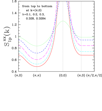
Figure 1: (Color online) $S_{\rm 1p}^{xx}({\bf k})$ along high-symmetry cuts through the Brillouin zone for the transverse Ising model with coupling $\lambda=0.1$, 0.2, 0.3, 0.328, 0.3284 on the square lattice. (From ref. [5]).

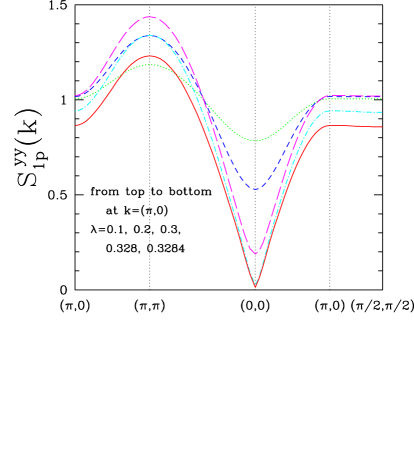
Figure 2: (Color online) $S_{\rm 1p}^{yy}({\bf k})$ along high-symmetry cuts through the Brillouin zone for the transverse Ising model with coupling $\lambda=0.1$, 0.2, 0.3, 0.328, 0.3284 on the square lattice. (From ref. [5]).

The behaviour of the transverse Ising model in higher dimensions is qualitatively similar. The 1-particle structure factors for the transverse Ising model on the triangular, square, and cubic lattices have also been calculated by Hamer et al. [5], using high-order series expansions. Some sample results for the square and cubic lattices are shown in Figures 2-4.

For the square lattice, the critical point is estimated [12] to lie at $\lambda=0.32841(2)$, and the critical exponents are expected to be the same as those of the classical 3D Ising model, namely $\eta=0.0364(5)$, $\nu=0.6301(4)$, from various estimates [13]. The results for $S_{\rm 1p}^{xx}$ and $S_{\rm 1p}^{yy}$ along high-symmetry cuts through the Brillouin zone for the system with couplings $\lambda=0.1$, 0.2, 0.3, 0.328 and 0.3284 are given in Figures 2 and 2. The results of a standard Dlog Padé analysis [5] of the series for $S^{xx}_{\rm 1p}({\bf k})$ at ${\bf k}=(0,0)$ and ${\bf k}=(\pi/2,\pi/2)$ at ${\bf k}=(0,0)$, where the energy gap vanishes, give estimates $\lambda_{c}=0.3284(4)$ with exponent $-0.605(5)$, compared to the expected exponent $\nu(\eta-1)=-0.607$. At momentum ${\bf k}=(\pi/2,\pi/2)$, where the energy gap remains finite, we find $\lambda_{c}=0.34(3)$ with exponent $0.04(2)$ compared to the expected value $\nu\eta=+0.0229$. For $S_{\rm 1p}^{yy}$, the estimate for the critical index is very close to the value $\nu(\eta+1)=0.65$.

In Figures 2 and 2 for $\lambda=0.328$ and 0.3284, we have biased the critical point to $\lambda_{c}=0.32841$ with critical index $\nu\eta=+0.0229$ in our analysis. We can see from these figures, that even for $\lambda=0.3284$ which is very close to the critical point, $S_{\rm 1p}^{xx}$ and $S_{\rm 1p}^{yy}$ are still far from zero. This reflects the tiny value of the exponent $\eta\nu$, which implies a precipitous drop to zero just before the critical point.

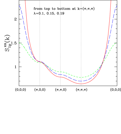
Figure 3: (Color online) $S_{\rm 1p}^{xx}({\bf k})$ along high-symmetry cuts through the Brillouin zone for the transverse Ising model with coupling $\lambda=0.1$, 0.15 and 0.19 on the simple cubic lattice. (From ref. [5]).

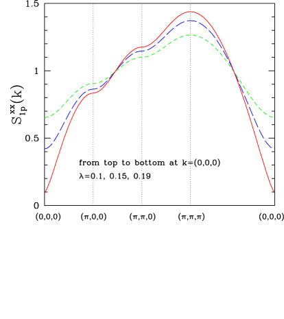
Figure 4: (Color online) $S_{\rm 1p}^{yy}({\bf k})$ along high-symmetry cuts through the Brillouin zone for the transverse Ising model with coupling $\lambda=0.1$, 0.5 and 0.19 on the simple cubic lattice. (From ref. [5]).

Figures 4 and 4 show similar graphs for the simple cubic lattice. In this case, the critical point has been obtained previously [14] as $\lambda_{c}=0.19406(6)$, and the critical exponents are expected to lie in the universality class of the 4D classical Ising model, where we expect the mean field exponents $\eta=0$ , $\nu=1/2$, modulo logarithmic corrections [4].

The analysis of $S^{xx}_{\rm 1p}({\bf k})$ at ${\bf k}=(0,0,0)$, where the energy gap vanishes, gives $\lambda_{c}=0.19406(8)$ with exponent $-0.54(1)$, while for $S^{yy}_{\rm 1p}({\bf k})$ at ${\bf k}=(0,0,0)$, the estimate of the critical point is $\lambda_{c}=0.194(4)$ with exponent $0.55(3)$. Away from ${\bf k}=(0,0,0)$, where the energy gap remains finite, we find $\lambda_{c}=0.22(3)$ with exponent $0.03(2)$ for both $S^{xx}_{\rm 1p}({\bf k})$ and $S^{yy}_{\rm 1p}({\bf k})$. Allowing for logarithmic corrections, these estimates agree reasonably well with the expected values.

In all cases, we see that the dominant structure factor $S^{xx}_{1p}$ at the critical wavevector diverges at the critical coupling with exponent $-\nu(1-\eta)$, while $S^{yy}_{1p}$ vanishes with exponent consistent with $\nu(1+\eta)$. Away from the critical wavevector, the structure factors both vanish at the critical coupling with a small exponent consistent with $\nu\eta$.

4.2 The Alternating Heisenberg Chain

Schmidt and Uhrig [6] and Hamer et al. [7] have investigated the spectral weights of the alternating Heisenberg chain, which can be described by the following Hamiltonian

$$H=\sum_{i}\left({\bf S}_{2i}\cdot{\bf S}_{2i+1}+\lambda{\bf S}_{2i-1}\cdot{\bf S}_{2i}\right)$$ (54)

where the ${\bf S}_{i}$ are spin-$\frac{1}{2}$ operators at site $i$, and $\lambda$ is the alternating coupling. Here we assume that the distance between neighboring spins are all equal and the distance between two successive dimers is $d$.

There is a considerable literature on this model, which has been reviewed by Barnes et al. [15]. At $\lambda=0$, the system consists of a chain of decoupled dimers, and in the ground state each dimer is in a singlet state. Excited states are made up from the three triplet excited states on each dimer, with a finite energy gap between the singlet ground state and the triplet excited states. This scenario is believed [16, 17, 18] to hold right up to the uniform limit $\lambda=1$, which corresponds to a critical point. At $\lambda=1$, we regain the uniform Heisenberg chain, which is gapless.

Several theoretical papers [19, 20, 21, 22] have discussed the approach to the uniform limit. Analytic studies of the critical behaviour near $\lambda=1$ [19] have related the alternating chain to the 4-state Potts model, and indicate that the ground-state energy per site $\epsilon_{0}(\lambda)$, and the energy gap $\Delta(\lambda)$ should behave as

$$\epsilon_{0}(\lambda)-\epsilon_{0}(1) \sim \delta^{4/3}/|\ln(\delta/\delta_{0})|$$ (55)

$$\Delta(\lambda) \sim \delta^{2/3}/\sqrt{|\ln(\delta/\delta_{0})|}$$ (56)

as $\lambda\to 1$, where $\delta=(1-\lambda)/(1+\lambda)$. This corresponds to critical exponents $\alpha=2/3$, $\nu=2/3$. The logarithmic terms in (53) are due to the existence of a marginal variable in the model.

For the uniform chain $\lambda=1$, and near $kd\to 2\pi$, Affleck [23] has obtained expressions for the correlation functions in the model, including logarithmic corrections, which correspond to an exponent $\eta=1$:

$$G^{z}(r)=G^{x}(r)\rightarrow\frac{1}{(2\pi)^{3/2}}\frac{(\ln r)^{1/2}}{r}.$$ (57)

Fourier transforming, one obtains the asymptotic form for $S^{-+}(kd)$ as

$$S(kd)\equiv S^{-+}(kd)=\frac{8}{3(2\pi)^{3/2}}|\ln(\pi-kd/2)|^{3/2}$$ (58)

Note that in this case $(1-\eta)\nu=0$, so there is no power-law divergence in the structure factor, but rather a logarithmic one.

This implies that for $kd=2\pi$ and as $\lambda\to 1$, the asymptotic form for $S(2\pi)$ diverges as

$$S(2\pi)\propto[-\ln(1-\lambda)]^{3/2}\quad\lambda\to 1$$ (59)

For $0<kd<2\pi$, one expects $S$ to be finite for any $\lambda$.

The results obtained by Hamer et al. [7] for $S$ versus momentum $k$ for $\lambda=0$, 0.6, and 1 are shown in Fig. 6. Note that $\int_{0}^{2\pi}S(k)dk=2\pi$ (here we set $d=1$), independent of $\lambda$, so the area under each curve is the same. Also shown in the figure are the results for $S^{\prime}\equiv 6S[-2\pi\ln(1-\frac{k}{2\pi})/k]^{-3/2}$ at $\lambda=1$. The results appear reasonably consistent with the expected behaviour.

Figure 5: The integrated structure factor $S$ versus $k$ for the alternating Heisenberg chain with $\lambda=0$ (dotted line), 0.6 (dashed line), 1 (crosses). Also shown is the quantity $S^{\prime}\equiv 6S[-2\pi\ln(1-\frac{k}{2\pi})/k]^{-3/2}$ for $\lambda=1$ (squares). (From ref. [7]).

Figure 6: The integrated structure factor $S$ versus $\lambda$ for the alternating Heisenberg chain with $kd=\pi/2$, $\pi$, $3\pi/2$ and $2\pi$. (From ref. [7]).

For fixed values of $k$, Fig. 6 shows the integrated structure factor $S$ versus $\lambda$, where for each value of $k$, about 20 different integrated differential approximants to the series are shown. We can see that the results converge very well out to $\lambda=1$. The logarithmic divergence as $\lambda\to 1$ for the case $kd=2\pi$ is clearly evident.

For $0<kd<2\pi$, an analysis of the series for the 1-particle structure factor $S_{\rm 1p}\equiv S^{-+}_{1p}$ using Dlog Padé approximants by Schmidt and Uhrig [6] appeared to show that it vanishes with a behavior close to $(1-\lambda)^{1/3}$. Since $S$ remains finite, one would thus expect that $S_{\rm 1p}/S$ vanishes like $(1-\lambda)^{1/3}$. This agrees with a heuristic argument [6] that the 1-particle spectral weight should vanish like $\sqrt{\Delta}$, i.e. like $\delta^{1/3}/|\ln(\delta/\delta_{0})|^{1/4}$, where $\delta=(1-\lambda)/(1+\lambda)$. It disagrees, however, with what one might expect from the transverse Ising model example, that the one-particle residue should vanish with exponent $\eta\nu=2/3$ at all wavevectors, leading to a behaviour $(1-\lambda)^{2/3}$. It is possible that a logarithmic correction term may again be disguising the true power-law behaviour; or alternatively, the power-law behaviour of the renormalized one-particle residue function might indeed be different away from the critical wavevector. It would be useful to have some further analytical guidance in this case.

Fig. 8 shows numerical values from Hamer et al. [7] for the relative 1-particle weight $S_{\rm 1p}/S$ versus $\lambda$ at selected values of $kd$. It can be seen that for any non-zero value of $k$, $S_{\rm 1p}/S$ decreases abruptly to zero as $\lambda\to 1$. Only at $kd=0+$, does $S_{\rm 1p}/S$ remain finite (about 0.993) in the limit $\lambda=1$; but by then $S$ has itself decreased to zero.

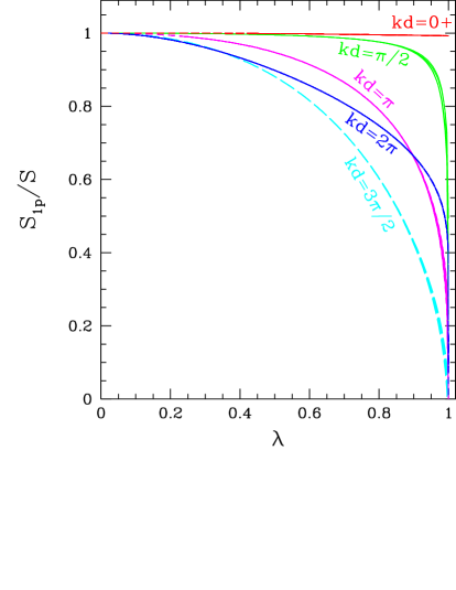
Figure 7: The relative 1-particle weight $S_{\rm 1p}/S$ versus $\lambda$ for the alternating Heisenberg chain with $kd=0+$, $\pi/2$, $\pi$, $3\pi/2$ and $2\pi$. (From ref. [7]).

Figure 8: The auto correlation functions versus $\lambda$ of the bilayer Heisenberg model for the 1-particle state ($\Phi_{\rm 1p}$), 2-particle states ($\Phi_{\rm 2p}$), and two particle bound states $T_{1}$ and $T_{2}$. (From ref. [8]).

Finally, we discuss the results for the spin auto-correlation functions, defined as

$$\Phi(\omega)=\frac{1}{2\pi}\int^{\infty}_{-\infty}dkS^{-+}(k,\omega)$$ (60)

Schmidt and Uhrig [6] argued that the critical behaviour for the total auto correlation function (summed over $\omega$) of the 1-particle state $\Phi_{\rm 1p}$ should be

$$\Phi_{\rm 1p} \propto (1-\lambda)^{1/3}$$ (61)

modulo logarithms, as for the structure factors.

Figure 8 shows various auto-correlation functions versus $\lambda$, reproduced from Hamer et al.. One can see that $\Phi_{\rm 1p}$ vanishes at the limit $\lambda=1$, while $(1-\lambda)^{-1/3}\Phi_{\rm 1p}$ increases almost linearly as $\lambda$ increases. The curve for $(\Phi_{\rm 1p}+\Phi_{\rm 2p})$, if we assume it is non-singular at $\lambda=1$ (i.e. the singularities in $\Phi_{\rm 1p}$ and $\Phi_{\rm 2p}$ cancel exactly), runs almost flat with $\lambda$ once we neglect unphysical and defective approximants: that would indicate that the 2-particle sector accounts for about 99.8% of the weight, even at $\lambda=1$, which agrees almost exactly with the conclusions of Schmidt and Uhrig [6]. Remarkably, this is much higher than the fraction of 73% for the two-spinon continuum at $\lambda=1$ calculated by Karbach et al. [24] from the exact solution. Also shown in Fig. 8 is the direct extrapolation of the 2-particle auto-correlation $\Phi_{\rm 2p}$ using integrated differential approximants. These extrapolations assume that there is no singularity in $\Phi_{\rm 2p}$ at $\lambda=1$, and the results give a somewhat smaller value of about 0.9 at $\lambda=1$.

Overall, then, the 1-particle energy gap and spectral weight at general momenta appear to vanish as $\lambda\to 1$, following the behaviour predicted by Cross and Fisher [19], and already confirmed numerically by Singh and Zheng [25]. However, the 2-triplet spectral weight remains finite in the uniform limit and, in fact, appears to form the major part of the total spectral weight. Schmidt and Uhrig [6] already pointed out that indeed the 2-triplet states carry a larger portion of the total spectral weight than the 2-spinon states, calculated by Karbach et al. [24]. This argues that a description in terms of triplons remains equally valid with a description in terms of spinons for the uniform chain.

4.3 Heisenberg Bilayer Model

As our final example, we consider the Heisenberg bilayer antiferromagnet on the square lattice, with Hamiltonian

$$H=J_{1}\sum_{l\ =\ 1,2}\sum_{<i,j>}{\bf S_{li}\cdot S_{lj}}+J_{2}\sum_{i}{\bf S_{1i}\cdot S_{2i}}$$ (62)

where $l=1,2$ labels the two planes of the bilayer. The physics of the system then depends on the coupling ratio $\lambda=J_{1}/J_{2}$. At $\lambda=0$, the ground state consists simply of $S=0$ dimers on each bond between the two layers, and excitations are composed of $S=1$ ‘triplon’ states [6] on one or more bonds. At large $\lambda$, where the $J_{1}$ interaction is dominant, the ground state will be a standard Néel state, with $S=1$ ‘magnon’ excitations. At some intermediate critical value $\lambda_{c}$, a phase transition will occur between these two phases. It is believed that this transition is of second order, and is accompanied by a Bose-Einstein condensation of triplons/magnons in the ground state.

Figures 10 and 10 show some series results for structure factors in the dimerized phase, calculated by Collins and Hamer [8]. Figure 10 shows the total static transverse structure factor $S({\bf k})\equiv S^{+-}({\bf k})$ as a function of ${\bf k}$ at various couplings $\lambda=J_{1}/J_{2}$. All results are for $k_{z}=\pi$, probing intermediate states antisymmetric between the planes, and we only refer to ${\bf k}=(k_{x},k_{y})$ hereafter.

The dominant feature is a large peak at the Néel point ${\bf k}=(\pi,\pi)$, which appears to become divergent as $\lambda\rightarrow\lambda_{c}$, as we would expect. Figure 10 shows the ratio of the 1-particle structure factor $S_{1p}({\bf k})$ to the total $S({\bf k})$ as a function of ${\bf k}$. The 1-particle contribution generally remains the dominant part of the total, particularly near the Néel point.

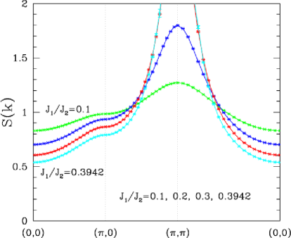
Figure 9: The total static structure factor $S({\bf k})$ in the bilayer Heisenberg model as a function of ${\bf k}$ at various couplings $\lambda=J_{1}/J_{2}$. (From ref. [8]).

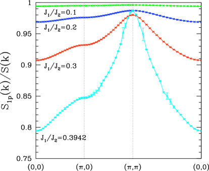
Figure 10: The ratio $S_{1p}({\bf k})/S({\bf k})$ of the 1-particle static structure factor to the total static structure factor as a function of ${\bf k}$ in the bilayer Heisenberg model, for various couplings $\lambda=J_{1}/J_{2}$. (From ref. [8]).

Let us now compare these results with theoretical expectations. From scaling theory (Sec. 2), both the 1-particle structure factor and the total structure factor in the vicinity of the critical point should scale like $(\lambda_{c}-\lambda)^{(\eta-1)\nu}$, at the critical (Néel) momentum. We expect this transition to belong to the universality class of the O(3) model in 3 dimensions, which has critical exponents [26] $\nu=0.707(4)$, $\eta=0.036(3)$, hence we expect $(\eta-1)\nu=-0.682(5)$, which is quite compatible with the numerical estimates.

How does $S_{1p}$ behave at the critical coupling away from the Néel momentum? Here the behaviour is quite different from the previous models. The ratio $S_{1p}/S$ decreases smoothly towards the critical coupling, and shows no sign of vanishing there. In fact the 1-particle structure factor remains dominant everywhere, remaing at 80% of the total or more. Thus it appears that in this case the renormalized residue function does not vanish at $\lambda_{c}$, except at the Néel momentum.

5 Summary and Conclusions

This paper consists largely of a review of the behaviour of structure factors near a quantum phase transition, at temperature $T=0$. We have focused here on quantum spin models, but the conclusions should apply more generally.

Section 2 reviewed current theory on the subject, drawn largely from Sachdev [4]. The generic scaling behaviour of both the total structure factor and the 1-particle exclusive structure factor is predicted to be the same, determined by the critical exponents $\eta$ and $\nu$.

We then reviewed calculations of the structure factors for some specific quantum spin models. For the transverse Ising model in one dimension, exact results can be obtained [5]; while for the transverse Ising model in higher dimensions [5], the alternating Heisenberg chain [6, 7], and the bilayer Heisenberg model [8], we have used some numerical results obtained from series expansions to high orders. For the most part, the results conform to theoretical expectations.

Some significant differences have been noted, however, in the detailed behaviour of these models, particularly as regards the 1-particle structure factor. In the transverse Ising model the 1-particle residue vanishes at the critical point for all wavevectors, and so the 1-particle contribution to the total structure factor becomes negligible. For the solvable case of the one-dimensional chain, the residue is actually independent of wavevector.

For the alternating chain, the one-particle residue again vanishes at the critical point, and it is the 2-particle ‘triplon’ state which appears to become dominant at the phase transition [6, 7]. But the residue appears to vanish with a different exponent depending on the wavevector, namely 2/3 at the critical wavevector and 1/3 away from it, which seems peculiar. It could be that the true exponent is disguised by logarithmic corrections, or perhaps the renormalized residue function does indeed behave differently at different wavevectors, and vanishes with a subdominant exponent away from the critical wavevector. Further analysis is needed here.

For the bilayer Heisenberg model, on the other hand, the renormalized 1-particle residue vanishes at the critical wavevector only, and the 1-particle state remains dominant at the critical point. This is presumably the more typical pattern of behaviour.

References

References

- [*] Email address: c.hamer@unsw.edu.au
- [1] Tennant D A, Broholm C, Reich D A, Nagler S E, Granroth G E, Barnes T, Damle K, Xu G, Chen Y and Sales B C 2003 Phys. Rev.B 67 054414
- [2] Marshall W and Lovesey S W 1971 Theory of Thermal Neutron Scattering: the Use of Neutrons for the Investigation of Condensed Matter (Oxford: Clarendon Press)
- [3] Als-Nielsen J 1976 in ’Phase Transitions and Critical Phenomena’ (New York: Academic) ed. Domb C and Green M S Vol. 5a p. 88.
- [4] Sachdev S 1999 Quantum Phase Transitions (Cambridge : Cambridge University Press)
-
[5]
Hamer C J, Oitmaa J, Zheng W-H and McKenzie R 2006 Phys. Rev.B 74 060402
Hamer C J, Oitmaa J and Zheng W-H 2006 Phys. Rev.B 74 174428 - [6] Schmidt K P and Uhrig G S 2003 Phys. Rev. Lett.90 227204
- [7] Hamer C J, Zheng W-H and Singh R R P 2003 Phys. Rev.B 68 214408
- [8] Collins A and Hamer C J 2008 Phys. Rev.B 78 054419
- [9] Cardy J, 1996 Scaling and Renormalization in Statistical Physics (Cambridge: Cambridge Uniersity Press)
- [10] Pfeuty P, 1970 Ann. Phys., NY57 79
- [11] Vaidya H C and Tracy C A 1978 Physica 92 A 1
- [12] Hamer C J 2000 J. Phys. A: Math. Gen.33 6683
- [13] Pelissetto A, Vicari E 2002 Physics Reports 368 549
- [14] Zheng W-H, Oitmaa J and Hamer C J 1994 J. Phys. A: Math. Gen.27 5425
- [15] Barnes T, Riera T and Tennant D A 1999 Phys. Rev.B 59 11384
- [16] Duffy W and Bair K P 1968 Phys. Rev.165 647
- [17] Bonner J and Blöte H W J 1982 Phys. Rev.B 25 6959
- [18] Jiang X-F, Chen H and Xing D Y 2001 J. Phys. A: Math. Gen.34 L259
-
[19]
den Nijs M P M 1979 Physica 95 A 449
Cross M C and Fisher D 1979 Phys. Rev.B 19 402
Black J L and Emery V J 1981 Phys. Rev.B 23 429 -
[20]
Uhrig G S, Schönfeld F, Laukamp M and Dagotto E 1999 Eur. Phys. J.
B 7 67
Papenbrock T, BarnesT, Dean D J , Stoitsev M V and Stayer M R cond-mat/0212254. -
[21]
Sorenson E S, Affleck I, Augier D and Poilblanc D 1998 Phys. Rev.B
58 R14701
Affleck I 1997 in Dynamical Properties of Unconventional Magnetic Systems (NATO ASI, Geilo, Norway) -
[22]
Essler F H L, Tsvelik A M and Delfino G 1997 Phys. Rev.B
56 11001
see also Gogolin A O, Nersesyan A A and Tsvelik A M 1998 Bosonization and strongly correlated systems (Cambridge: Cambridge University Press) - [23] Affleck I 1998 J. Phys. A: Math. Gen.31 4573
- [24] Karbach M, Müller G and Bougourzi A M 1997 Phys. Rev.B 55 12510
- [25] Singh R R P and Zheng W-H 1999 Phys. Rev.B 59 9911
- [26] Guida R and Zinn-Justin J 1998 J. Phys. A: Math. Gen.31 8103