Local molecular field theory for the treatment of electrostatics

Abstract

We examine in detail the theoretical underpinnings of previous successful applications of local molecular field (LMF) theory to charged systems. LMF theory generally accounts for the averaged effects of long-ranged components of the intermolecular interactions by using an effective or restructured external field. The derivation starts from the exact Yvon-Born Green hierarchy and shows that the approximation can be very accurate when the interactions averaged over are slowly varying at characteristic nearest-neighbor distances. Application of LMF theory to Coulomb interactions alone allows for great simplifications of the governing equations. LMF theory then reduces to a single equation for a restructured electrostatic potential that satisfies Poisson’s equation defined with a smoothed charge density. Because of this charge smoothing by a Gaussian of width $\sigma$, this equation may be solved more simply than the detailed simulation geometry might suggest. Proper choice of the smoothing length $\sigma$ plays a major role in ensuring the accuracy of this approximation. We examine the results of a basic confinement of water between corrugated wall and justify the simple LMF equation used in a previous publication. We further generalize these results to confinements that include fixed charges in order to demonstrate the broader impact of charge smoothing by $\sigma$. The slowly-varying part of the restructured electrostatic potential will be more symmetric than the local details of confinements.

I Introduction

The treatment of long-ranged Coulomb interactions remains a substantial challenge in nearly all classical molecular simulations. The basic problem is that interactions from even very distant charges remain important, as indicated by the divergence of the integral of 1/r from any finite truncation distance to infinity. This causes problems in computer simulations of systems with charges, where contributions from distant periodic images of the simulation cell must be taken into account, typically by Ewald sum techniques. This also hampers the development of simple, intuitive local pictures and analytic theory when charges are present.

Here we discuss basic features of a new approach for charged systems, local molecular field (LMF) theory. LMF theory was originally applied to Lennard-Jones (LJ) systems for both simulation and analytical work WeeksVollmayrKatsov.1997.Intermolecular-forces-and-the-structure-of-uniform-and-nonuniform ; WeeksKatsovVollmayr.1998.Roles-of-repulsive-and-attractive-forces-in-determining ; Vollmayr-LKatsovWeeks.2001.Using-mean-field-theory-to-determine ; KatsovWeeks.2001.Density-fluctuations-and-the-structure-of-a-nonuniform-hard ; KatsovWeeks.2001.On-the-mean-field-treatment-of-attractive-interactions ; Weeks.2002.Connecting , and the LMF approach has been used recently to analyze many charged systems, both uniform and nonuniform, with even greater success ChenKaurWeeks.2004.Connecting-systems-with-short-and-long ; ChenWeeks.2006.Local-molecular-field-theory-for-effective ; RodgersKaurChen.2006.Attraction-between-like-charged-walls:-Short-ranged ; DenesyukWeeks.2008.A-new-approach-for-efficient-simulation-of-Coulomb-interactions ; RodgersWeeks.2008.Interplay-of-local-hydrogen-bonding-and-long-ranged-dipolar .

LMF theory can be generally characterized as a mapping that relates structural and thermodynamic properties of a nonuniform system with long-ranged and slowly-varying intermolecular interactions in a given external potential energy field, representing, e.g., fixed solutes or confining walls, to those of a simpler “mimic system” with properly chosen short-ranged intermolecular interactions in an effective or restructured field. The strong short-ranged interactions in the mimic system are chosen to give an accurate description of the forces between typical nearest-neighbor molecules in the full system, e.g., the repulsive molecular cores in a dense LJ fluid, local hydrogen bonds in water, or ion pairs in a strongly coupled ionic system. Because of the short range of the interactions in the mimic system, fast and efficient simulations scaling linearly with system size are possible. The restructured field is determined self-consistently and is the sum of the bare external field in the original system and a density-weighted mean-field average of the remaining long-ranged and slowly-varying parts of the intermolecular interactions. The restructured field corrects major errors that can arise, especially in nonuniform systems, from applying solely a spherical truncation of the intermolecular pair interactions, exemplified by shifted force truncations for nonuniform Coulomb systems FellerPastorRojnuckari.1996.Effect-of-Electrostatic-Force-Truncation-on-Interfacial ; Spohr.1997.Effect-of-Electrostatic-Boundary-Conditions-and-System . More advanced spherical truncations of $1/r$ exist, such as site-site reaction field techniques HummerSoumpasisNeumann.1994.Computer-simulation-of-aqueous-Na-Cl-Electrolytes , but the difficulties in nonuniform situations remain the same.

The LMF approach offers a very general perspective and the averaging can be carried out for any slowly-varying component of the intermolecular interactions. We show here that LMF theory takes an especially powerful and simple form, with strong analogies to classical electrostatics, when it is applied uniformly to the basic Coulomb $1/r$ interaction alone (and not, e.g., to LJ interactions as well). We can then take advantage of symmetries between charges of different signs and magnitudes, interacting with the same spherically symmetric $1/r$ potential, and determine the effective field using only the total charge density, and not separate number densities for each charged species or interaction site as would be required for a general mixture. We find that the contribution to the restructured field in LMF theory from the slowly-varying parts of the Coulomb interactions can be exactly determined from a restructured electrostatic potential that satisfied Poisson’s equation, but with a Gaussian-smoothed charge distribution. A proper choice of the smoothing length $\sigma$ in the Gaussian plays a key role in the accuracy of LMF theory, since it also determines the size of the local strong-coupling region within which strong forces from nearest-neighbor sites must be accurately captured by the short-ranged interactions in the mimic system.

Previous discussions of LMF theory for Coulomb or LJ systems relied on general arguments and did not exploit all the important simplifications that arise by applying LMF theory only to $1/r$ with the same potential splitting regardless of point charge details. Here we seek to justify and document LMF theory as completely as possible, accounting for Coulomb symmetries. We show how this leads to a simple, broadly applicable equation for a restructured electrostatic potential, and then we extend results from RodgersWeeks.2008.Interplay-of-local-hydrogen-bonding-and-long-ranged-dipolar to show that smooth LMF solutions can still arise from a general class of molecularly-corrugated confinement potentials.

II Derivation of the LMF Equation

The LMF equation may be derived for mixtures and standard site-site molecular models. However the basic features of the derivation are identical regardless of whether we consider a mixture, a site-site molecular fluid, or a single-component system. Therefore, we present the derivation for a single-component system in order to highlight the physical approximations in the derivation without the clutter of the multiple indices necessary in the derivations for mixtures or molecules. Furthermore, symmetries available to us when treating charge interactions will allow us to simplify the LMF equation for mixtures into a single electrostatic potential equation, as we will show later in section III.

II.1 Motivation

We assume that the intermolecular interactions $w(r)$ in the full system of interest are slowly varying at large separations. The first step in LMF theory is to divide $w(r)$ into properly chosen short- and long-ranged parts:

$$w(r)=u_{0}(r)+u_{1}(r),$$ (1)

such that $u_{1}(r)$ contains all the the slowly-varying long-ranged interactions in $w(r)$ but remains slowly varying at characteristic nearest-neighbor distances where there are strong forces between neighboring molecules. By construction, the short-ranged component $u_{0}(r)$ then captures those strong short-ranged forces but vanishes quickly at larger separations.

LMF theory then defines a mapping from the full system with pair potential $w(r)$ and an external single-particle potential energy function $\phi(\mathbf{r})$ to a mimic system defined by the short-ranged pair interactions $u_{0}(r)$ and an effective or restructured external potential energy function $\phi_{\rm R}(\mathbf{r})$:

$$\begin{array}[]{ccc}\mbox{Full}&&\mbox{Mimic}\\ \left\{\begin{array}[]{c}w(r)\\ \phi(\mathbf{r})\end{array}\right\}&\stackrel{{\scriptstyle\mathrm{LMF}}}{{\rightarrow}}&\left\{\begin{array}[]{c}u_{0}(r)\\ \phi_{\rm R}(\mathbf{r})\end{array}\right\}.\end{array}$$ (2)

We call the final combination a mimic system when $u_{0}(r)$ and $\phi_{\rm R}$ are properly chosen because we seek a system that can capture many relevant structural and thermodynamic properties of the full system. In addition, we seek this mapping to be closed, in the sense that the mapping should not require any information about the full system other than the original $w(r)$ and $\phi(\mathbf{r})$. It seems plausible that some effective $\phi_{\rm R}$ could account for averaged effects of the neglected long-ranged interactions $u_{1}(r)$ in the mimic system, but we seek a more careful development of this intuition.

II.2 Exact Starting Point for the LMF Derivation

The derivation of the LMF equation starts with an exact statistical mechanical equation involving structure and forces, the Yvon-Born-Green (YBG) hierarchy of equations McQuarrie.2000.Statistical-Mechanics ; HansenMcDonald.2006.Theory-of-Simple-Liquids . In one form, the first equation in the hierarchy reads

$$k_{\rm B}T\vec{\nabla}\ln\rho^{(1)}\left(\mathbf{\mathbf{r}}\right)=-\vec{\nabla}\phi(\mathbf{r})-\int d\mathbf{r}^{\prime}\rho\left(\mathbf{\mathbf{r}^{\prime}}\middle|\mathbf{\mathbf{r}}\right)\vec{\nabla}w\left(\left|\mathbf{r}-\mathbf{r^{\prime}}\right|\right).$$ (3)

This equation relates the gradient of the (singlet) density profile of the system, $\rho^{(1)}\left(\mathbf{\mathbf{r}}\right)$, to the force from the external single particle potential, $\phi(\mathbf{r})$, and the averaged force between particles, weighted by the conditional singlet density, $\rho\left(\mathbf{\mathbf{r}^{\prime}}\middle|\mathbf{\mathbf{r}}\right)$. This function $\rho\left(\mathbf{\mathbf{r}^{\prime}}\middle|\mathbf{\mathbf{r}}\right)$ is defined as the density at position $\mathbf{r}^{\prime}$ given that a particle is at $\mathbf{r}$, and may be expressed mathematically as the ratio of the two-particle density at $\mathbf{r}$ and $\mathbf{r^{\prime}}$ and the single-particle density at $\mathbf{r}$:

$$\rho\left(\mathbf{\mathbf{r}^{\prime}}\middle|\mathbf{\mathbf{r}}\right)\equiv\frac{\rho^{(2)}(\mathbf{r},\mathbf{r}^{\prime})}{\rho^{(1)}(\mathbf{r})}.$$ (4)

Thus, the YBG hierarchy expresses the rapidly-varying singlet density in terms of the more complex and even more rapidly-varying two-particle density. There are two related difficulties in trying to extract practically useful information about the singlet density from (3). First, the density profile is related to more complicated rapidly-varying functions. Second, there is no obvious manner to create a self-contained loop to determine the singlet density profile, again due to its relation to the higher-order density profile.

Typical superposition closures of the YBG hierarchy attempt to resolve both difficulties by approximating $\rho\left(\mathbf{\mathbf{r}^{\prime}}\middle|\mathbf{\mathbf{r}}\right)\simeq\rho^{(1)}\left(\mathbf{\mathbf{r}^{\prime}}\right)$, leading to an equation where the gradient over $\mathbf{r}$ can be pulled out of (3) and $\rho^{(1)}\left(\mathbf{\mathbf{r}}\right)$ is defined in terms of itself. However, even for a bulk fluid, this is a poor approximation for any moderately dense liquid KrumhanslWang.1972.Superposition-assumption.-I.-Low-density-fluid-argon ; WangKrumhansl.1972.Superposition-assumption.-2.-High-density-fluid-argon . The superposition approximation neglects any excluded volume or specific-binding interactions that alter the small $\left|\mathbf{r}-\mathbf{r^{\prime}}\right|$ nature of $\rho\left(\mathbf{\mathbf{r}^{\prime}}\middle|\mathbf{\mathbf{r}}\right)$ relative to $\rho^{(1)}\left(\mathbf{\mathbf{r}^{\prime}}\right)$. Replacing the conditional singlet density with the singlet density simplifies the equation but also effectively includes with large weight too many configurations where two particles are improbably close to each other, leading to great inaccuracies.

We assume that there exists a good choice of $u_{0}(r)$ that captures those short-ranged excluded-volume and specific-binding contributions. We will describe such a choice ChenKaurWeeks.2004.Connecting-systems-with-short-and-long for splitting $1/r$ using the smoothing length $\sigma$ in section III. Given $u_{0}(r)$, we write the YBG equations for both the full sytem and the LMF-mapped system, denoted by the subscript R, from (2) as:

$$k_{\rm B}T\vec{\nabla}\ln\rho^{(1)}\left(\mathbf{\mathbf{r};[\phi]}\right)=-\vec{\nabla}\phi(\mathbf{r})$$

$$\qquad\qquad-\int d\mathbf{r}^{\prime}\rho\left(\mathbf{\mathbf{r}^{\prime}}\middle|\mathbf{\mathbf{r};[\phi]}\right)\vec{\nabla}w\left(\left|\mathbf{r}-\mathbf{r^{\prime}}\right|\right),$$

$$k_{\rm B}T\vec{\nabla}\ln\rho^{(1)}_{\rm R}\left(\mathbf{r};[\phi_{\rm R}]\right)=-\vec{\nabla}\phi_{\rm R}(\mathbf{r})$$

$$\qquad\qquad-\int d\mathbf{r}^{\prime}\rho_{\rm R}\left(\mathbf{r}^{\prime}\middle|\mathbf{r};[\phi_{\rm R}]\right)\vec{\nabla}u_{0}\left(\left|\mathbf{r}-\mathbf{r^{\prime}}\right|\right).$$ (5)

The density profiles and conditional singlet densities are written as functionals of $\phi(\mathbf{r})$ and $\phi_{\rm R}(\mathbf{r})$ to emphasize the restructuring of the external potential energy in the LMF mapping.

As written with an arbitrary choice of $u_{0}(r)$, (5) simply displays formally exact but not particularly useful equations for two arbitrary and unconnected systems with different intermolecular interactions in different external fields. As in WeeksKatsovVollmayr.1998.Roles-of-repulsive-and-attractive-forces-in-determining , we now connect these systems and achieve substantial simplifications and cancellations by requiring that $\phi_{\rm R}$ be chosen so that

$$\rho^{(1)}(\mathbf{r};[\phi])=\rho_{\rm R}^{(1)}(\mathbf{r};[\phi_{\rm R}]).$$ (6)

It seems very plausible that such a $\phi_{\rm R}$ exists, especially when $u_{0}(r)$ captures the strong short-ranged intermolecular forces. We then take the difference between the equations in (5). The terms involving the singlet densities on the left-hand sides cancel and the result can be exactly written in a form useful for further analysis as

$$-\vec{\nabla}\phi_{\rm R}(\mathbf{r})=-\vec{\nabla}\phi(\mathbf{r})-\int d\mathbf{r}^{\prime}\rho_{\rm R}(\mathbf{r}^{\prime};[\phi_{\rm R}])\vec{\nabla}u_{1}\left(\left|\mathbf{r}-\mathbf{r^{\prime}}\right|\right)$$ (7a)

$$\qquad-\int d\mathbf{r}^{\prime}\left[\rho(\mathbf{r}^{\prime}|\mathbf{r};[\phi])-\rho_{\rm R}(\mathbf{r}^{\prime}|\mathbf{r};[\phi_{\rm R}])\right]\vec{\nabla}u_{0}\left(\left|\mathbf{r}-\mathbf{r^{\prime}}\right|\right)$$ (7b)

$$\qquad-\int d\mathbf{r}^{\prime}\left[\rho(\mathbf{r}^{\prime}|\mathbf{r};[\phi])-\rho(\mathbf{r}^{\prime};[\phi])\right]\vec{\nabla}u_{1}\left(\left|\mathbf{r}-\mathbf{r^{\prime}}\right|\right).$$ (7c)

Henceforth, for simplicity, we denote $\rho^{(1)}\left(\mathbf{\mathbf{r}}\right)$ as $\rho(\mathbf{r})$.

Equation (7) formally holds for any choice of $u_{0}(r)$ and $u_{1}(r)$, and because conditional densities still appear, it generally has most of the problems of the standard hierarchy equations noted after (4). Thus it may seem we have made little progress. But this is not the case for proper choice of $u_{0}(r)$ and $u_{1}(r)$ with the properties sketched above. This will allow considerable simplification of (7) and defines a mimic system that

• has a well-chosen $u_{0}(r)$ that mimics higher order correlations in the full system as well as the singlet density profile,

• can be treated via statistical mechanics without any a priori knowledge of the full system aside from $\phi(\mathbf{r})$ and $w(r)$, and

• has an associated $\phi_{\rm R}(\mathbf{r})$ that depends only on singlet density profiles of the mimic system and not on the more complex conditional singlet densities.

II.3 Approximations to Yield LMF Equation

Physically-motivated approximations to the exact (7) will result in a final LMF equation below in (8) that has a simple mean-field form. The following discussion elucidates that the LMF equation is not a blind assertion of mean-field behavior but rather a controlled and accurate approximation, provided that we choose our mimic system carefully.

Recalling from (1) that $w(r)=u_{0}(r)+u_{1}(r)$, the LMF derivation focuses on making two connected and physically-reasonable approximations based on choosing a short-ranged $u_{0}(r)$ that will induce the correct nearest-neighbor structure, where the conditional singlet and singlet densities differ the most, and a corresponding $u_{1}(r)$ that is slowly-varying on that length scale. As we will see in section III.1, the form of the Coulomb potential grants us the freedom to fulfill both conditions by choosing a single smoothing length $\sigma$. When $u_{0}(r)$ and $u_{1}(r)$ are chosen correctly, we shall have a “mimic system.”

By making approximations to (7), the equality of densities expressed in (6) will only hold approximately, and we will find an equation based on the exact (7) that will also no longer be exact. But all will be accurately satisfied with proper choices of $u_{0}(r)$ and $u_{1}(r)$. The general arguments below have been briefly sketched before WeeksKatsovVollmayr.1998.Roles-of-repulsive-and-attractive-forces-in-determining , but the form of (7) allows us to make a more precise statement of the necessary approximations.

We note that (7a) depends only on the density response of the mimic system, and no information about the density response of the full system or any conditional density is needed. Thus if terms (7b) and (7c) could be neglected, then (7a) alone would define a closed equation for the mimic system. The right side of (7a) still transforms as a gradient and should display all the associated properties. In that sense, neglecting terms (7b) and (7c) together may well be more accurate than taking either one of the following approximations individually.

With proper choice of $u_{0}(r)$ and $u_{1}(r)$, we may reasonably neglect the final two terms in (7) using the following arguments:

1. Term (7b) probes the difference between the conditional singlet densities for the full and mimic systems via convolution with $\vec{\nabla}u_{0}(r)$. The integrand will be quickly forced to zero at larger $\left|\mathbf{r}-\mathbf{r^{\prime}}\right|$ by the vanishing gradient of the short-ranged $u_{0}\left(\left|\mathbf{r}-\mathbf{r^{\prime}}\right|\right)$. Since both the full and mimic systems have the same strong short-ranged core forces with an appropriately chosen $u_{0}(r)$, and these core forces should mainly determine the short-ranged part of the conditional densities, it seems plausible that with proper choice of $u_{0}(r)$, term (7b) can be neglected. This is significantly better than any superposition approximation for the conditional densities and does not require us to numerically estimate either conditional density.

2. Term (7c) probes the difference between the conditional singlet density and the singlet density of the full system. As explained previously with relation to standard closures of the YBG equation, assuming their equality can be highly problematic at short distances. However, we are saved by the fact that this difference is paired with $\vec{\nabla}u_{1}\left(\left|\mathbf{r}-\mathbf{r^{\prime}}\right|\right)$. Since $u_{0}(r)$ has been chosen to encompass core interactions, $u_{1}(r)$ will be simultaneously slowly-varying over those nearest-neighbor distances, so the associated force is essentially zero for exactly the range of distances where the conditional singlet density and singlet density differ significantly. Thus we expect for many liquids that the integrand in term (7c) may also be accurately approximated as zero.

These two approximations allow us to truncate the YBG hierarchy. No explicit knowledge of the conditional singlet density in either the full or the mimic system will be required, but we expect the conditional singlet density of the mimic system to closely resemble that of the full system at short range.

Notably, the second approximation will fail when there are long-ranged pair correlations arising from capillary waves at the liquid-vapor interface or the divergence of the correlation length near the critical point. In those instances, the conditional singlet density will not be approximately the same as the singlet density well beyond nearest-neighbor distances. However, we do expect this approximation to hold in strongly-coupled charged systems away from the critical point where there exist pair correlations that decay exponentially over those nearest-neighbor distances.

With these two coupled approximations, only (7a) remains, and we can take the gradient with respect to $\mathbf{r}$ outside of the integral. Then, integrating over $\mathbf{r}$ yields the general LMF equation

$$\phi_{\rm R}(\mathbf{r})=\phi(\mathbf{r})+\int d\mathbf{r}^{\prime}\rho_{\rm R}(\mathbf{r}^{\prime};[\phi_{\rm R}])u_{1}\left(\left|\mathbf{r}-\mathbf{r}^{\prime}\right|\right)+C,$$ (8)

where the integration constant $C$ will be set by boundary conditions. The form of this equation highlights the connection with mean-field techniques. The function $\phi_{\rm R}$ may be viewed as an averaging of the slowly-varying, long-ranged portions of the pair potential over the single-particle density $\rho_{\rm R}(\mathbf{r})$. The hierarchy has been successfully truncated since $\phi_{\rm R}$ is defined in terms of only $\rho_{\rm R}(\mathbf{r})$. Provided sufficient computer time to simulate the short-ranged mimic system and therefore close the self-consistent loop between $\phi_{\rm R}(\mathbf{r})$ and $\rho_{\rm R}(\mathbf{r})$, the LMF equation is exactly soluble.

This equation is not a naïve mean-field ansatz for $\phi_{\rm R}$ since it arises from reasonable approximations to exact statistical mechanical equations. The crux of LMF theory, however, is choosing reasonable $u_{0}(r)$ and $u_{1}(r)$ such that the necessary approximations are accurate. The next section discusses this choice for $1/r$.

III Electrostatics via LMF Theory

Here, we explain our choice of $u_{0}(r)$ and $u_{1}(r)$ for charge interactions. Then, we seek to highlight the symmetry and simplifications possible when applying the LMF equation to purely charge-charge interactions by developing the LMF equation for a single restructured electrostatic potential, rather than for separate potential energy functions for each atom type.

III.1 Coulomb Potential Split

In CGS units, the pair interaction between two charges, $q_{\alpha}$ and $q_{\gamma}$, is

$$w(r)=\frac{q_{\alpha}q_{\gamma}}{\epsilon r}.$$ (9)

The factor $\epsilon$ is simply the dielectric constant of a uniform medium in which the charges are immersed. The details of charge magnitudes, signs, and choice of CGS or SI units will change from system to system, but the underlying functional form $1/r$ will remain constant. Thus, following DenesyukWeeks.2008.A-new-approach-for-efficient-simulation-of-Coulomb-interactions , we introduce $v_{0}(r)$ and $v_{1}(r)$ to split this function as

$$\frac{1}{r}\equiv v_{0}(r)+v_{1}(r),$$ (10)

into short-ranged and long-ranged components. Both $v_{0}(r)$ and $v_{1}(r)$ will yield either a potential energy or an electrostatic potential, with appropriate prefactors.

Work of previous researchers ChenKaurWeeks.2004.Connecting-systems-with-short-and-long revealed that a beneficial choice of $v_{1}(r)$ is the functional form associated with the electrostatic potential due to a unit Gaussian charge distribution of width $\sigma$, defined as

$$\rho_{G}(\mathbf{r})=\frac{1}{\pi^{3/2}\sigma^{3}}\exp\left(-\frac{r^{2}}{\sigma^{2}}\right),$$ (11)

leading to a $v_{1}(r)$ given by

$$v_{1}(r)\equiv\int d\mathbf{r}^{\prime}\rho_{G}(\mathbf{r^{\prime}})\cdot\frac{1}{\left|\mathbf{r}-\mathbf{r^{\prime}}\right|}=\frac{\mathop{\rm erf}(r/\sigma)}{r}~{}.$$ (12)

This $v_{1}(r)$ is slowly-varying in $r$-space over the smoothing length $\sigma$. As discussed in ChenKaurWeeks.2004.Connecting-systems-with-short-and-long , this choice of $v_{1}(r)$ also simultaneously isolates only the small wave-vector components of the Coulomb potential. The Fourier transform of $v_{1}(r)$ is

$$\hat{v}_{1}(k)=\frac{4\pi}{k^{2}}e^{-k^{2}\sigma^{2}/4},$$ (13)

and the Gaussian function attenuates any large-$k$ components that would be rapidly-varying in $r$-space. Thus the $v_{1}(r)$ is particularly well-suited for mean-field averaging.

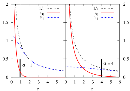
Figure 1: Demonstration of $1/r$ potential split for two different values of the smoothing length $\sigma$. When $\sigma$ is increased from 1 to 4, more of the $1/r$ core interaction is included in $v_{0}(r)$, and $v_{1}(r)$ becomes correspondingly more slowly varying.

The $v_{0}(r)$ corresponding to our choice of $v_{1}(r)$ will then be given as

$$v_{0}(r)\ =\frac{\mathop{\rm erfc}(r/\sigma)}{r}.$$ (14)

Therefore, $v_{0}(r)\equiv 1/r-v_{1}(r)$ is proportional to the electrostatic potential due to a point charge screened by a surrounding, neutralizing Gaussian charge distribution whose width $\sigma$ also sets the scale for the smooth truncation of $v_{0}(r)$. This split is shown in figure 1 along with a demonstration of the impact of increasing the smoothing length $\sigma$ on $v_{0}(r)$ and $v_{1}(r)$. The form of $v_{1}(r)$ is slowly varying over $\sigma$, and $v_{0}(r)$ approximately represents a Coulomb core potential of range $\sigma$. Tuning $\sigma$ to larger values increases the range of $v_{0}(r)$ and simultaneously smooths the variation of $v_{1}(r)$ over characteristic nearest-neighbor interactions.

Since $1/r$ has no inherent length scale, the split between short- and long-ranged by the smoothing length $\sigma$ may be tailored to each situation. This length $\sigma$ should not be viewed as a fitting parameter, but rather a consistency parameter. We expect that choosing $\sigma$ too small will result in poor and rapidly-varying results from full LMF theory as $\sigma$ is changed since the mean-field average will be over rapidly-varying interactions. However once $\sigma$ reaches a $\sigma_{\rm min}$ that is related to characteristic nearest-neighbor distances, the assumptions used in the previous section to derive the LMF equation from the YBG hierarchy become accurate, and essentially the same results should be found for larger $\sigma$ values as well oldfootnote . Thus we expect that self-consistently applied LMF theory with an appropriately chosen $\sigma$ will yield a true mimic system. This requirement for reasonable core inclusion has been explored in previous papers ChenKaurWeeks.2004.Connecting-systems-with-short-and-long ; ChenWeeks.2006.Local-molecular-field-theory-for-effective ; RodgersKaurChen.2006.Attraction-between-like-charged-walls:-Short-ranged .

For small $r<\sigma$, the force due to $v_{0}(r)$ is quite similar to that of a bare point charge. By increasing $\sigma$, we increase the effective range of these essentially unscreened Coulomb interactions. Thus, $v_{0}(r)$ can be thought of as a Gaussian-truncated (GT) or “short” Coulomb interaction. We refer to a model with generically-truncated Coulomb interactions as a short model and with $v_{0}(r)$ specifically used as a GT model. We showed in RodgersWeeks.2008.Interplay-of-local-hydrogen-bonding-and-long-ranged-dipolar that short GT water, where all the point charges in SPC/E water are replaced by $v_{0}(r)$ with no account taken of the effective field, can give a surprisingly accurate description of all site-site correlations for bulk water. But this same approach can fail spectacularly for electrostatic correlations in nonuniform systems unless corrected by the inclusion of the long-ranged forces via the LMF-restructured potential RodgersWeeks.2008.Interplay-of-local-hydrogen-bonding-and-long-ranged-dipolar .

The functional form of $v_{0}(r)$ suggests both Ewald sums Ewald.1921.Evaluation-of-optical-and-electrostatic-lattice-potentials and Wolf sums WolfKeblinskiPhillpot.1999.Exact-method-for-the-simulation-of-Coulombic-systems . Ewald sums, however, seek to explicitly evaluate the forces from $v_{1}(r)$ at each timestep using an exact sum over the fluctuating periodic images of the simulation cell, and thus have a very different philosophical approach. The analogy with Wolf sums is much more appropriate in that each results in a spherical truncation $v_{0}(r)$ applied at each time step. However, the historical development of the Wolf summation technique relies on the observation that charges in ionic lattices are quickly neutralized by slightly shifted “mirror” lattices of neutralizing charges. In fluids, this is altered to assuming that charges within a sharp cutoff radius are exactly neutralized by a shell of charge at the cutoff radius, and the use of $\mathop{\rm erfc}(r/\sigma)$ to damp the forces from $1/r$ is applied more as a numerical afterthought. In the context of LMF theory, we view such damping as much more crucial to the success of Wolf sums in reproducing the structure of uniform fluids than the imposition of strict neutrality within a sharp cutoff radius.

The GT $v_{0}(r)$ also bears great similarity to site-site reaction field (RF) approaches HummerSoumpasisNeumann.1994.Computer-simulation-of-aqueous-Na-Cl-Electrolytes ; Neumann.1983.Dipole-Moment-Fluctation-Formulas-in-Computer ; HummerSoumpasisNeumann.1992.Pair-correlations-in-an-NaCl-SPC-water-model ; HummerSoumpasis.1994.Computation-of-the-Water-Density-Distribution-at-the-Ice-WaterInterface , when the fluid is assumed to be conducting. The usual RF method generates a truncated $v_{0,{\rm RF}}(r)$ from the electrostatic potential of a unit point charge surrounded by a uniform neutralizing spherical charge distribution. We discuss in the Appendix more details of the relation between the GT $v_{0}(r)$, and the usual RF $v_{0,{\rm RF}}(r)$ as well as a smoother charged-clouds RF truncation $v_{0,{\rm CC}}(r)$ HummerSoumpasisNeumann.1994.Computer-simulation-of-aqueous-Na-Cl-Electrolytes . The choice of spheres as the neutralizing charge distribution in these RF methods leads to a potential that is exactly zero beyond a certain cutoff distance, but this induces a discontinuity in a higher order derivative at the sharp cutoff. The LMF choice of Gaussians leads to an infinitely smooth and soft truncation both in $r$-space and $k$-space. Moreover a GT model logically separates the choice of the smoothing length $\sigma$ from the possible use for computational convenience of a sharp cutoff at a larger distance along with various local smoothing schemes that could be employed near the cutoff.

Despite the general similarities, the theoretical constructs of both reaction field techniques and Wolf sums allow for no obvious correction in nonuniform systems, such as the slab confinement to which we applied LMF theory in RodgersWeeks.2008.Interplay-of-local-hydrogen-bonding-and-long-ranged-dipolar . As such, LMF theory is an important advance in the use of spherical truncations for $1/r$.

III.2 LMF Electrostatic Potential

Now we will derive a further simplified electrostatic form of the LMF equation. We need only consider the LMF mixture equation here because, with appropriate further approximations, the LMF equation for standard molecular models collapses onto the mixture LMF equation as will be shown in a paper dealing more broadly with site-site molecular models HuRodgersWeeks.. . Using the YBG equation for mixtures, exactly the same approximations as in section II lead to the following LMF equation for a species $\alpha$ in a mixture of different species indexed by $\gamma$ and including $\alpha$, as originally given in ChenWeeks.2006.Local-molecular-field-theory-for-effective :

$$\phi_{R,\alpha}=\phi_{\alpha}(\mathbf{r})+\sum_{\gamma}\int d\mathbf{r}^{\prime}\,\rho_{R,\gamma}(\mathbf{r}^{\prime})\cdot u_{1,\alpha\gamma}(\left|\mathbf{r}-\mathbf{r^{\prime}}\right|).$$ (15)

If the pair interactions being treated were of general form this would be the furthest simplification possible, with an LMF equation to be solved for each different species.

The observation in ChenWeeks.2006.Local-molecular-field-theory-for-effective that a single $\sigma$ for all charged interactions proves most useful leads straightforwardly to a much more compact form. Using the LMF approach only for charges, each $u_{1,\alpha\gamma}(r)$ may be written as

$$u_{1,\alpha\gamma}(r)=\frac{q_{\alpha}q_{\gamma}}{\epsilon}\frac{\mathop{\rm erf}\left(r/\sigma\right)}{r}=\frac{q_{\alpha}q_{\gamma}}{\epsilon}v_{1}(r).$$ (16)

Thus (15) may be exactly written as

$$\phi_{{\rm R},\alpha}(\mathbf{r})=\phi_{\alpha}(\mathbf{r})+\frac{q_{\alpha}}{\epsilon}\int d\mathbf{r}^{\prime}\,\left(\sum_{\gamma}q_{\gamma}\rho_{{\rm R},\gamma}(\mathbf{r}^{\prime})\right)\cdot v_{1}(\left|\mathbf{r}-\mathbf{r^{\prime}}\right|).$$ (17)

Using the natural definition of charge density as

$$\rho^{q}(\mathbf{r})=\sum_{\gamma}q_{\gamma}\rho_{\gamma}(\mathbf{r}),$$ (18)

we may reexpress the previous equation for $\phi_{{\rm R},\alpha}$ as

$$\phi_{{\rm R},\alpha}(\mathbf{r})=\phi_{\alpha}(\mathbf{r})+\frac{q_{\alpha}}{\epsilon}\int d\mathbf{r}^{\prime}\,\rho^{q}_{\rm R}(\mathbf{r}^{\prime})\cdot v_{1}(\left|\mathbf{r}-\mathbf{r^{\prime}}\right|).$$ (19)

By noting as done in ChenWeeks.2006.Local-molecular-field-theory-for-effective that $\phi_{\alpha}$ may be due to both electrostatic and nonelectrostatic components, we separate $\phi_{\alpha}$ as

$$\phi_{\alpha}(\mathbf{r})=\phi_{{\rm ne},\alpha}(\mathbf{r})+q_{\alpha}\mathcal{V}(\mathbf{r})$$ (20)

where $\phi_{{\rm ne},\alpha}$ encompases nonelectrostatic confinements such as the smooth LJ walls used in RodgersWeeks.2008.Interplay-of-local-hydrogen-bonding-and-long-ranged-dipolar and $\mathcal{V}$ represents the general external electrostatic potential.

This observation naturally leads to the following rewriting of each LMF equation for a species $\alpha$ as

$$\phi_{{\rm R},\alpha}(\mathbf{r})=\phi_{{\rm ne},\alpha}(\mathbf{r})+q_{\alpha}\mathcal{V}_{\rm R}(\mathbf{r}),$$ (21)

with a single restructured electrostatic potential $\mathcal{V}_{\rm R}$, defined as

$$\mathcal{V}_{\rm R}(\mathbf{r})=\mathcal{V}(\mathbf{r})+\frac{1}{\epsilon}\int d\mathbf{r}^{\prime}\rho^{q}_{\rm R}(\mathbf{r}^{\prime})\cdot v_{1}(\left|\mathbf{r}-\mathbf{r^{\prime}}\right|).$$ (22)

Thus all self-consistent requirements on the diverse set of $\phi_{{\rm R},\alpha}$ can be written in terms of a single restructured electrostatic potential $\mathcal{V}_{\rm R}$ defined by one LMF equation involving the equilibrium mobile charge density $\rho^{q}$.

Given the convolution definition of $v_{1}(r)$ as the potential due to a Gaussian charge density in (12), we may schematically represent the integral term in (22) as $\rho^{q}$$\ast$$\rho_{G}$$\ast$$1/r$ where $\ast$ indicates a convolution. Thus (22) can be exactly rewritten as

$$\mathcal{V}_{\rm R}(\mathbf{r})=\mathcal{V}(\mathbf{r})+\frac{1}{\epsilon}\int d\mathbf{r}^{\prime}\,\rho^{q_{\sigma}}_{\rm R}(\mathbf{r}^{\prime})\cdot\frac{1}{\left|\mathbf{r}-\mathbf{r^{\prime}}\right|},$$ (23)

where $\rho^{q_{\sigma}}$ represents the smoothing of the charge density by $\rho_{G}$ in (11) via the convolution

$$\rho^{q_{\sigma}}(\mathbf{r})\equiv\int d\mathbf{r}^{\prime}\,\rho^{q}(\mathbf{r}^{\prime})\rho_{G}(\left|\mathbf{r}-\mathbf{r^{\prime}}\right|).$$ (24)

In almost all cases of interest we can picture $\mathcal{V}$ as arising from a fixed, external charge distribution $\rho^{q}_{\rm ext}$, and we should apply the same separation of the Coulomb potential to the fixed as well as mobile charges. This will allow us to express (23) in a suggestive and compact form using the sum of the fixed charge density and the equilibrated mobile charge density profile, $\rho^{q}_{\rm tot}(\mathbf{r})=\rho^{q}(\mathbf{r})+\rho^{q}_{\rm ext}(\mathbf{r})$. Thus we write

$$\mathcal{V}(\mathbf{r})=\mathcal{V}_{0}(\mathbf{r})+\mathcal{V}_{1}(\mathbf{r}).$$ (25)

Just as $v_{1}(r)$ is the electrostatic potential due to a point charge convolved with a Gaussian of width $\sigma$, so $\mathcal{V}_{1}$ is the electrostatic potential due to the convolution of the fixed external charge density $\rho^{q}_{\rm ext}$ with that same Gaussian as defined in (11) and used in (12) and (24). Given the definition of $\mathcal{V}_{0}$ and $\mathcal{V}_{1}$, we write analogously

$$\mathcal{V}_{\rm R}(\mathbf{r})=\mathcal{V}_{0}(\mathbf{r})+\mathcal{V}_{\rm R1}(\mathbf{r}),$$ (26)

thus defining $\mathcal{V}_{\rm R1}(\mathbf{r})$, the slowly-varying component of the restructured electrostatic potential.

Using (23), this slowly-varying component is exactly given by

$$\mathcal{V}_{\rm R1}(\mathbf{r})=\frac{1}{\epsilon}\int d\mathbf{r}^{\prime}\,\rho^{q_{\sigma}}_{\rm R,tot}(\mathbf{r}^{\prime})\cdot\frac{1}{\left|\mathbf{r}-\mathbf{r^{\prime}}\right|}.$$ (27)

We see that $\mathcal{V}_{\rm R1}$ is the electrostatic potential arising from the Gaussian smoothing of the total charge density, $\rho^{q_{\sigma}}_{\rm tot}(\mathbf{r})$.

Equation (27) appears as the standard definition of the electrostatic potential due to charge density from first-year textbooks like Purcell.1985.Electricity-and-Magnetism . Thus the LMF equation for the slowly-varying component of the restructured electrostatic potential may be viewed as simply doing classical electrostatics on an equilibrium, smoothed total charge density and defining a single external restructured electrostatic potential. In fact we may in general represent the slowly-varying LMF equation (27) as a modified Poisson’s equation,

$$\vec{\nabla}^{2}\mathcal{V}_{\rm R1}(\mathbf{r})=-\frac{4\pi}{\epsilon}\rho^{q_{\sigma}}_{\rm R,tot}(\mathbf{r}),$$ (28)

based on the smoothed total charge density. This point was first made for the uniformly-charged-wall model system Chen.2004.General-Theory-of-Nonuniform-Fluids:-From , and it is immediately generalizable to the LMF equation dealt with here. The existence of this Poisson-like equation dictating a modified electrostatics emphasizes that, in order for LMF theory to be valid for electrostatics, all charge-charge interactions, whether fixed, bound, or mobile, should be mapped via LMF theory to short-ranged interactions in the restructured electrostatic potential $\mathcal{V}_{\rm R}$. In RodgersWeeks.2008.Interplay-of-local-hydrogen-bonding-and-long-ranged-dipolar , we emphasized the value of this modified-electrostatics perspective in physically interpreting molecular simulations and in understanding why and when spherical Gaussian truncations, using $v_{0}(r)$ alone, fail in nonuniform environments.

IV Further Simplifications Due to Charge Smoothing

Understanding the LMF equation as standard electrostatics for a Gaussian-smoothed charge density also allows for simpler solutions of the LMF equation than might be initially expected. As an example, in RodgersWeeks.2008.Interplay-of-local-hydrogen-bonding-and-long-ranged-dipolar , we were able to use a one-dimensional LMF equation to treat a system that has a charge density profile with an explicitly three-dimensional character. In this section, we give the reasoning behind such simplifications and argue that they should be expected generally in many physically relevant cases.

IV.1 Simple Corrugated Surface

In RodgersWeeks.2008.Interplay-of-local-hydrogen-bonding-and-long-ranged-dipolar , we treated SPC/E water confined to a slab by two empirical Pt(111) surfaces RaghavanFosterMotakabbir.1991.Structure-and-Dynamics-of-Water-at-the-Pt111-Interface: that order the water molecules at the surface, attracting the oxygen atoms to localized binding sites. Details of the simulation methods are available in RodgersWeeks.2008.Interplay-of-local-hydrogen-bonding-and-long-ranged-dipolar . In brief, we simulated 1054 SPC/E molecules confined between the two walls with 500 ps of equilibration and 1.5 ns of subsequent data collection. Simulations using slab-corrected three-dimensional Ewald sums, LMF theory with $\sigma=4.5$ Å, and LMF theory with $\sigma=6.0$ Å were carried out. During those runs, the timestep chosen was 1.0 fs. However, for self-consistent solution of the LMF equation, we first simulated sets of 10 shorter runs with 25 ps of equilibration and 50 ps of accumulation with a timestep of 2.5 fs. These 10 shorter runs began with distinct initial conditions; we observed that averaging the $\rho^{q}$ resulting from such a set of simulations better isolated the system’s equilibrium response to changes in $\mathcal{V}_{\rm R}$ from the natural fluctuations in the charge density. For the larger $\sigma$, convergence was achieved within 3 iterations, and for the smaller $\sigma$, 10 iterations were required for self-consistency. This approach certainly does not represent a numerically optimized solution of the LMF equation and is used here only to demonstrate the accuracy possible in principle when the full LMF theory is used. We will address the need for a more comprehensive and numerically efficient approach to the solution of the LMF equation and general timing issues further in section V.

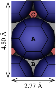
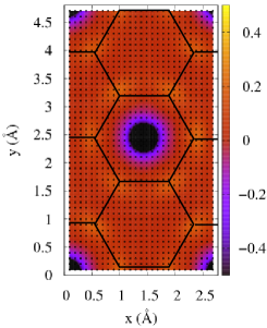
Figure 2: A (111) surface and the proximal charge density. 2 Sketch of the rectangular unit cell for a (111) surface showing the topmost three layers of atoms, labelled A, B, and C. 2 Corresponding $\rho^{q}(x,y)$ in e₀/ų for the 1.5 Å layer closest to the wall. The density is projected onto the $xy$-plane, and the grayscale (color online) indicates the value of the charge at each point. Black dots indicate collected data points.

In contrast to the smooth hydrophobic surface also dealt with in that paper, the empirical (111) surface was intended to represent detailed and specific ordering of water molecules at an atomically-corrugated surface. A schematic of the rectangular unit cell of a (111) surface is shown in figure 2, demonstrating the spacing of the three topmost layers of atoms. The empirical Pt(111) potential RaghavanFosterMotakabbir.1991.Structure-and-Dynamics-of-Water-at-the-Pt111-Interface: that we use does not have explicit atoms or charges. Rather the potential simply encompasses the presence of binding sites through exponential functions and various cosine functions to represent the periodicity of the surface.

As expected from the form of the potential, the charge density $\rho^{q}$ depends on $x$ and $y$ in addition to $z$. In figure 2, the charge density $\rho^{q}(x,y)$ in the 1.5 Å layer nearest the (111)-wall is projected onto a unit cell. As previously demonstrated RaghavanFosterMotakabbir.1991.Structure-and-Dynamics-of-Water-at-the-Pt111-Interface: , the surface induces a charge density profile very nonuniform in the $x$- and $y$-directions. The distinct periodicity is due to the fact that the spacing between binding sites (2.77 Å) is nearly commensurate with the first peak in the bulk water $g_{\rm OO}(r)$ ($\sim$ 2.8 Å). However despite a charge density that was explicitly a function of $\mathbf{r}$, we obtained accurate results for system properties using $\mathcal{V}_{\rm R}(z)$ RodgersWeeks.2008.Interplay-of-local-hydrogen-bonding-and-long-ranged-dipolar . We posited that this was the case due to the charge smoothing described in the previous section.

Here we seek to demonstrate this more quantitatively by probing the charge density profile away from the surface within hexagonal prisms defined by three distinct hexagonal binding regions – A, B, and C – as labeled in figure 2. Figure 3(a) shows the $\rho^{q}(z)$ measured along each hexagonal prism and averaged laterally over the hexagonal area. These density profiles are quite distinct both from each other and from the full laterally-smoothed $\rho^{q}(z)$.

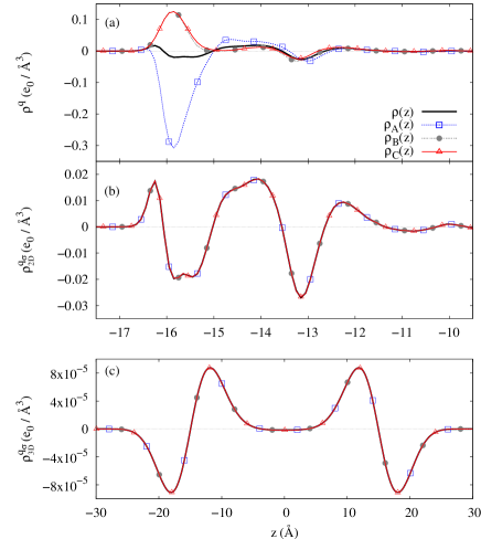
Figure 3: Effect of smoothing with a Gaussian of width $\sigma=4.5$ Å on $\rho^{q}(\mathbf{r})$ between two empirical (111) walls. (a) The charge density $\rho^{q}(z)$ for the three hexagonal prisms labeled A, B, and C in figure 2. (b) Gaussian smoothing of these density profiles in the $x$- and $y$-directions. (c) Full three-dimensional Gaussian smoothing of the $\rho^{q}(z)$ profiles. The plots in (a) and (b) focus on data near the left wall, but the plot in (c) displays data for the full slab of water between the walls.

The Gaussian smoothing of charge density inherent in the LMF treatment allows us to distinguish the coherent and incoherent variations in charge density seen in figure 3(a). As shown in figure 3(b), convoluting $\rho^{q}(\mathbf{r})$ with Gaussians in the $x$- and $y$-directions and subsequently analyzing sites A, B, and C leads to a density, $\rho^{q_{\sigma}}_{2D}$, that is indistinguishable from the $\rho^{q}(z)$ calculated initially as only a function of $z$. This equivalence is due to that fact that the corrugations in effect induce local random noise in the density profile that is therefore averaged out by the Gaussians of width greater than the corrugation. In contrast, the presence of the confining surface leads to a $\rho^{q_{\sigma}}$ density profile that does not average out in the $z$-direction as seen in figure 3c. In essence, the LMF smoothing approach shows when variations in charge density profiles cancel, and when they do not.

IV.2 Simplifications Still Hold For Surfaces with Fixed Charges

However, a reasonable criticism of the previous surface is that it was not atomically realistic, even on a classical level. More realistic metallic surfaces would require a treatment of image charges, which we will not address here. However, molecular surfaces modeled with standard force fields would at least have charges at atomic sites near the surface. If the charges are free to move throughout the simulation as would generally be the case for biological membranes or liquid-liquid interfaces, absolutely no change in tactic would be necessary. The charges associated with those molecules would also be included in the mobile $\rho^{q}$.

If, instead, the charges are held fixed, as is more likely for solid surfaces in classical simulations of solid-liquid interfaces, then $\phi_{\alpha}(\mathbf{r})=\phi_{\alpha,{\rm ne}}(\mathbf{r})+q_{\alpha}\mathcal{V}(\mathbf{r})$. In such cases, we may no longer approximation $\mathcal{V}_{\rm R}(\mathbf{r})$ as $\mathcal{V}_{\rm R}(z)$, but a similar simplification for the smooth $\mathcal{V}_{\rm R1}$ will hold, as might be expected. Such a potential for silica surfaces GiovambattRosskyDebenedett.2006.Effect-of-pressure-on-the-phase-behavior-and-structure is currently being employed in our group to study the silica-acetonitrile interface HuUnpub .

For surfaces with fixed charges, the imposed external electrostatic potential $\mathcal{V}(\mathbf{r})$ would be

$$\mathcal{V}(\mathbf{r})={\sum_{{\rm sites}\,i}}^{\prime}\frac{q_{i}}{\epsilon\left|\mathbf{r}-\mathbf{r_{i}}\right|},$$ (29)

where the prime indicates that these surface charges will need to be accounted for in the surface extending to infinity in the $x$- and $y$-directions. The pair interactions representing the excluded volume of these atomic sites would be included in $\phi_{{\rm ne},\alpha}$. The external electrostatic potential $\mathcal{V}$ may be split into short-ranged component $\mathcal{V}_{0}$ and long-ranged component $\mathcal{V}_{1}$ as

$$\mathcal{V}_{0}(\mathbf{r})=\sum_{{\rm sites}\,i}\frac{q_{i}}{\epsilon}v_{0}(\left|\mathbf{r}-\mathbf{r_{i}}\right|),$$ (30)

$$\mathcal{V}_{1}(\mathbf{r})={\sum_{{\rm sites}\,i}}^{\prime}\frac{q_{i}}{\epsilon}v_{1}(\left|\mathbf{r}-\mathbf{r_{i}}\right|).$$ (31)

Now $\mathcal{V}_{0}$ is a simple minimum image sum over short-ranged pair interactions. The long-ranged component $\mathcal{V}_{1}$ still must include the effect of surface sites extending out to infinity in the $x$- and $y$-directions, but since $\mathcal{V}_{1}$ may be interpreted as the electrostatic potential due to a Gaussian smoothing of the fixed charge sites, we expect that

$$\mathcal{V}_{1}(\mathbf{r})\simeq\mathcal{V}_{1}(z).$$ (32)

The sole requirement would be that $\sigma$ should be larger than relevant lateral spacing of sites on the surface, such that the charge density will be sufficiently smoothed in the lateral directions. In such a case, $\mathcal{V}_{\rm R}$ is a function of $\mathbf{r}$, but all dependence on $x$ and $y$ is contained in $\mathcal{V}_{0}(\mathbf{r})$, and we would expect the self-consistent $\mathcal{V}_{\rm R1}(z)$ to hold to a very good approximation.

As a quick demonstration of the validity of these ideas, we construct a (111)-surface with lattice constant $a=3.92$ Å as for the model (111)-surface discussed in section IV.1. However, we arbitrarily assign charges of $+1$ e₀ for the first layer of atoms, $-2$ e₀ for the second layer of atoms, and $+1$ e₀ for the third layer of atoms.

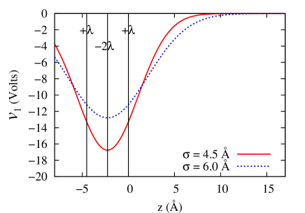
Figure 4: $\mathcal{V}_{1}(z)$ for charged (111)-surface for two different $\sigma$. This approximation to $\mathcal{V}_{1}(\mathbf{r})$ is nonnegligible within $2\sigma$ of the surface.

The corresponding $\mathcal{V}_{1}(z)$ would be determined by smoothing out the charges in each layer laterally, such that the charged (111)-surface is now approximated by three uniformly charged planes. With this representation, we may exactly express $\mathcal{V}_{1}(z)$ as the sum of three analytical functions,

$$\mathcal{V}_{1}(z)=\sum_{i\in{\rm layers}}\frac{2\pi\lambda_{i}}{\epsilon}G(z,z_{i}),$$ (33)

where $\lambda_{i}$ is the surface charge density of each layer, and $G$ is the one-dimensional Gaussian-smoothed Green’s function for a planar charge distribution ChenWeeks.2006.Local-molecular-field-theory-for-effective ; RodgersKaurChen.2006.Attraction-between-like-charged-walls:-Short-ranged analogous to $v_{1}(r)$  in Eq. (12) for a point charge.

$\mathcal{V}_{1}(z)$ is plotted in figure 4 and is an important contributor to the forces near the surface. However, since the surface is net neutral, it decays essentially to zero within a distance of approximately $2\sigma$ from the surface.

We may calculate both $\mathcal{V}(\mathbf{r})$ and $\mathcal{V}_{0}(\mathbf{r})$ easily by constructing various configurations of one $+1$ unit test charge above this (111)-surface in the dlpoly2.16 molecular dynamics package. We exactly calculate $\mathcal{V}_{0}(\mathbf{r})$ to within the simulation energy precision, by carrying out single point energy calculations for a $+1$ e₀ test charge above various $(x,y)$-sites interacting with each particle in the surface via $v_{0}(r)$. This particle is a test charge in the sense that it measures the $\mathcal{V}_{0}$ generated by the charges in the surface without disturbing the organization of charges within the surface. Thus the LMF estimation of the total $\mathcal{V}(\mathbf{r})$ is

$$\mathcal{V}(\mathbf{r})\simeq\mathcal{V}_{\rm LMF}(\mathbf{r})\simeq\mathcal{V}_{0}(\mathbf{r})+\mathcal{V}_{1}(z),$$ (34)

with $\mathcal{V}_{1}(z)$ given analytically by (33).

In order to determine $\mathcal{V}(\mathbf{r})$ independently, we employ slab-corrected three-dimensional Ewald sums as a way to estimate that function YehBerkowitz.1999.Ewald-summation-for-systems-with-slab . Since Ewald sums require net neutrality, we construct two surfaces with test charges – the surface we are interested in with a $+1$ test charge above it and a second mirror surface with opposite charges with a $-1$ test charge above it. The two (111)-surfaces have lateral size 30.49 Å $\times$ 28.806 Å with $L_{z}=280$ Å, and we use $\alpha=0.34$ Å^-1 and $\mathbf{k}_{\rm max}=(13,12,120)$ for the corrected three-dimensional Ewald sums. We separate the two surfaces within the simulation cell as much as possible in order to decouple each surface and test-charge pair from the other pair.

The energies yielded from these single-point-energy calculations $U_{\rm Ewald}(\mathbf{r})$ allow us to estimate $\mathcal{V}(\mathbf{r})$, provided that we subtract the contribution from test charge-test charge interactions $U_{+-}(z)$ and the constant contribution from intra-wall particle interactions ($U_{\rm wall}$) as follows,

$$\mathcal{V}(\mathbf{r})\simeq\mathcal{V}_{\rm Ewald}(\mathbf{r})=\frac{1}{2}\left\{U_{\rm Ewald}(\mathbf{r})-U_{+-}(z)-U_{\rm walls}\right\}.$$ (35)

This is approximate since the Ewald sums will propagate the test charges laterally into all the periodic image cells, but given that the lateral area spans $11\times 6$ repeats of the minimum rectangular (111)-surface unit cell of 2.77 Å $\times$ 4.80 Å, interactions between each surface and the lateral periodic images of the nearest test charge should be minimal.

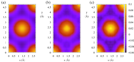
Figure 5: Electrostatic potential $\mathcal{V}(\mathbf{r})$ at a distance of 2.26 Å above the charged surface as calculated by (a) corrected three-dimensional Ewald sums and by LMF estimation with (b) $\sigma=4.5$ Å and (c) $\sigma=6.0$ Å. LMF estimation entails approximating $\mathcal{V}(\mathbf{r})$ as $\mathcal{V}_{0}(\mathbf{r})+\mathcal{V}_{1}(z)$.

Shown in figure 5 is $\mathcal{V}(x,y,z)$ for $z$ fixed at $2.26$ Å as treated by (a) Ewald sums, (b) the LMF approximation with $\sigma=4.5$ Å, and (c) the LMF approximation with $\sigma=6.0$ Å. The similarity of the electrostatic potential surface for each $\sigma$ to the full Ewald calculation demonstrates that 4.5 Å is greater than $\sigma_{\rm min}$ for the fixed surface at least. This stands to reason since, within a plane, particles are within 2.77 Å of each other and the planes of particles are separated by about 2.26 Å. Therefore $\sigma=4.5$ Å is greater than relevant particle spacings. The agreement between $\mathcal{V}_{\rm LMF}(\mathbf{r})$ and $\mathcal{V}_{\rm Ewald}(\mathbf{r})$ is expected but numerically nontrivial since $\left|\mathcal{V}_{1}\right|\gg\left|\mathcal{V}\right|$ at this distance above the surface. Therefore, achieving this degree of accuracy is a result of the accurate addition of two large-magnitude terms, $\mathcal{V}_{0}(\mathbf{r})$ and $\mathcal{V}_{1}(z)$, to yield a much smaller magnitude $\mathcal{V}_{\rm LMF}(\mathbf{r})$.

In order to demonstrate this agreement more broadly, we again study sites A, B, and C as shown in figure 2. Figure 6 shows the difference

$$\Delta\mathcal{V}(\mathbf{r})\equiv\mathcal{V}_{\rm Ewald}(\mathbf{r})-\mathcal{V}_{\rm LMF}(\mathbf{r}),$$ (36)

laterally averaged above each hexagonal site. This variation $\Delta\mathcal{V}(\mathbf{r})$ is relatively small for a $\sigma$ of either 4.5 Å or 6.0 Å since either $\sigma$ is greater than any relevant spacings in the surface. Compared to the huge discrepancies that would arise from using solely $\mathcal{V}_{0}(\mathbf{r})$ and neglecting the several Volt contribution of $\mathcal{V}_{1}(z)$, these differences are miniscule. At larger $z$, there are slightly larger variations, which we believe are numerical artifacts arising from our use of a sharp cutoff radius (10.5 Å for $\sigma=4.5$ Å and 13.5 Å for $\sigma=6.0$ Å) in $\mathcal{V}_{0}$. Given the small scale on these graphs, even very tiny errors will visibly accumulate.

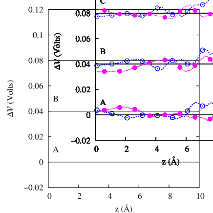
Figure 6: Plots of $\Delta\mathcal{V}(\mathbf{r})$ in Volts averaged above the sites A, B, and C as displayed in figure 2 for smoothing lengths $\sigma=4.5$ Å and $\sigma=6.0$ Å. Data for site B is displaced vertically by 0.04 Volts and data for site C by 0.08 Volts. In each case the value of $\mathcal{V}_{1}(z)$ is several volts, but the correction $\Delta\mathcal{V}(\mathbf{r})$ is substantially smaller.

We fully expect that we should be able to treat $\mathcal{V}_{\rm R}$ as

$$\mathcal{V}_{\rm R}(\mathbf{r})\simeq\mathcal{V}_{0}(\mathbf{r})+\mathcal{V}_{\rm R1}(z).$$ (37)

In fact, we expect this approximation for $\mathcal{V}_{\rm R1}$ to be even better than for $\mathcal{V}_{1}$ since the mobile charge density is included and will act to neutralize the fixed charged sites to an extent. The validity of approximating the Gaussian-smoothed equilibrium charge density profile $\rho^{q_{\sigma}}$ as solely a function of $z$ for non-electrostatic corrugated surface confinement discussed in section IV.1 should also hold for the mobile charge density profile in this model system with fixed point charges. Thus we conclude that this system should be treatable by LMF theory with the same one-dimensional equation as used in RodgersWeeks.2008.Interplay-of-local-hydrogen-bonding-and-long-ranged-dipolar with the sole difference that $\mathcal{V}_{0}$ is a function of $\mathbf{r}$.

V Conclusions and Outlook

Based on the success of LMF theory in treating a variety of charged and molecular systems ChenKaurWeeks.2004.Connecting-systems-with-short-and-long ; ChenWeeks.2006.Local-molecular-field-theory-for-effective ; RodgersKaurChen.2006.Attraction-between-like-charged-walls:-Short-ranged ; DenesyukWeeks.2008.A-new-approach-for-efficient-simulation-of-Coulomb-interactions ; RodgersWeeks.2008.Interplay-of-local-hydrogen-bonding-and-long-ranged-dipolar ; HuRodgersWeeks.. , we believe that LMF theory is a promising new approach that permits simple minimum-image simulations of $1/r$ interactions while still accurately accounting for the net additive long-ranged forces using the restructured external electrostatic potential $\mathcal{V}_{\rm R}$. While the systems treated thus far have been simple ionic and molecular systems, the LMF framework is much more broadly applicable to simulation systems of biomolecular and experimental interest. Current research using the LMF approach in the Weeks research group includes the collapse of model charged polymers DenesyukUnpub and the behavior of acetonitrile near silica surfaces HuUnpub .

Here we have sought to present the statistical mechanical foundations of the LMF treatment of charged systems. We have highlighted the necessary but physically reasonable approximations leading to the LMF equation, and we have also derived the simple LMF equation for the electrostatic potential valid when treating point-charge models, both ionic and molecular.

Furthermore, we have examined the useful consequences of understanding the smoothly-varying LMF electrostatic potential $\mathcal{V}_{\rm R1}$ as resulting from a Gaussian-smoothed charge density. In a previous paper RodgersWeeks.2008.Interplay-of-local-hydrogen-bonding-and-long-ranged-dipolar , we showed that this charge density can be physically enlightening. Here we instead show the practical utility of this smoothing. The convolution of the charge density with a Gaussian of width $\sigma$ allows us to solve much simpler LMF equations than might originally be believed. For confinement into a slab geometry, regardless of whether the confinement has nonelectrostatic or electrostatic corrugations, the relevant LMF equation will depend only on $z$ to a very good approximation.

In future work, we will examine the application of LMF theory to bulk site-site fluids in much more detail HuRodgersWeeks.. and also demonstrate very simple corrections that allow much more accurate thermodynamics from GT models RodgersWeeks.. . Another area which we hope to explore in greater detail is methods for optimally solving the LMF equation during simulation. As alluded to in RodgersWeeks.2008.Interplay-of-local-hydrogen-bonding-and-long-ranged-dipolar , the writing of the LMF equation as a Poisson equation with a Gaussian smoothed charge density suggests that connection with work on efficient Poisson solvers would be numerically helpful, and that simple approximations may prove surprisingly accurate DenesyukWeeks.2008.A-new-approach-for-efficient-simulation-of-Coulomb-interactions . Furthermore, since Poisson’s equation may be written as the minimum of a functional Jackson.1999.Classical-Electrodynamics , using a modified Car-Parinello scheme FrenkelSmit.2002.Understanding-Molecular-Simulation:-From-Algorithms to slowly evolve to the averaged, equilibrium solution of the LMF equation seems like another fruitful path to pursue. In our (unoptimized) simulations of LMF systems, we observed a speed-up of at least a factor of four relative to Ewald summation. However, such timing questions need to be studied in much greater detail once an optimized path to LMF solution is developed.

Regardless of such possibilities for solution of the LMF equation, LMF theory is still an inherently equilibrium theory. Given the success of a scaling principle of dynamics that states that equilibrium, dynamic properties will be well-captured in a reference system that reproduced static, structural properties YoungAndersen.2005.Tests-of-an-approximate-scaling-principle-for-dynamics , many dynamical properties for equilibrium systems could possibly be modeled quite well in our LMF-mapped systems. But such a conjecture needs to be tested, and, regardless, much further theoretical work is required to develop the analog of LMF theory for dynamically-evolving systems.

Appendix: Relation between the GT $v_{0}(r)$ and Reaction Field Truncations

The standard short-ranged RF pair interaction $v_{0,{\rm RF}}(|\mathbf{r}_{n}-\mathbf{r}_{t}|)$ is proportional to the potential energy between a unit point charge at $\mathbf{r}_{t}$ and a unit point charge at $\mathbf{r}_{n}$ surrounded by a uniform neutralizing spherical charge distribution terminating at the sharp cutoff radius $R_{c}$ of the RF model. Anticipating that we may want a more symmetric description of the charge distributions at $\mathbf{r}_{t}$ and $\mathbf{r}_{n}$, we can also relate the RF $v_{0,{\rm RF}}$ to the difference between the potential energy of two unit point charges at $\mathbf{r}_{t}$ and $\mathbf{r}_{n}$ and the potential energy of a unit uniform spherical charge distribution at $\mathbf{r}_{n}$ and a unit point charge at $\mathbf{r}_{t}$. But the subtracted term is not symmetric and the smoother charged-clouds interaction HummerSoumpasisNeumann.1994.Computer-simulation-of-aqueous-Na-Cl-Electrolytes $v_{0,{\rm CC}}(r)$ can be found by subtracting the potential energy of two unit uniform spherical charge distributions at $\mathbf{r}_{n}$ and $\mathbf{r}_{t}$ (with cutoff radius $R_{c}/2$) from the potential energy of two unit point charges at $\mathbf{r}_{t}$ and $\mathbf{r}_{n}$. The functional form $v_{0,{\rm CC}}(r)$ was previously arrived at via a less symmetric argument HummerSoumpasisNeumann.1994.Computer-simulation-of-aqueous-Na-Cl-Electrolytes . The functional form $v_{0,{\rm CC}}(r)$ is different than that of $v_{0,{\rm RF}}(r)$.

In contrast, the $v_{0}(|\mathbf{r}_{n}-\mathbf{r}_{t}|)=\mathop{\rm erfc}(|\mathbf{r}_{n}-\mathbf{r}_{t}|/\sigma)/|\mathbf{r}_{n}-\mathbf{r}_{t}|$ chosen for LMF theory can be related to either the energy between a unit point charge at $\mathbf{r}_{t}$ and a unit point charge at $\mathbf{r}_{n}$ surrounded by a neutralizing Gaussian charge distribution of width $\sigma$ or equivalently to the difference between the potential energy of two unit point charges at $\mathbf{r}_{t}$ and $\mathbf{r}_{n}$ and the potential energy of two unit Gaussian charge distributions of width $\sigma/\sqrt{2}$ at $\mathbf{r}_{n}$ and $\mathbf{r}_{t}$ ChenKaurWeeks.2004.Connecting-systems-with-short-and-long . The same functional form $v_{0}(r)=\mathop{\rm erfc}(r/\sigma)/r$ results in either case.

References

- (1) Weeks J D, Vollmayr K and Katsov K, 1997. Physica A 244 461
- (2) Weeks J D, Katsov K and Vollmayr K, 1998. Phys. Rev. Lett. 81 4400
- (3) Vollmayr-Lee K, Katsov K and Weeks J D, 2001. J. Chem. Phys. 114 416
- (4) Katsov K and Weeks J D, 2001. Phys. Rev. Lett. 86 440
- (5) Katsov K and Weeks J D, 2001. J. Phys. Chem. B 105 6738
- (6) Weeks J D, 2002. Annu. Rev. Phys. Chem. 53 533
- (7) Chen Y G, Kaur C and Weeks J D, 2004. J. Phys. Chem. B 108 19874
- (8) Chen Y G and Weeks J D, 2006. Proc. Nat. Acad. Sci. USA 103 7560
- (9) Rodgers J M, Kaur C, Chen Y G and Weeks J D, 2006. Phys. Rev. Lett. 97 097801
- (10) Denesyuk N A and Weeks J D, 2008. J. Chem. Phys. 128 124109
- (11) Rodgers J M and Weeks J D, submitted. Proc. Nat. Acad. Sci. USA
- (12) Feller S E, Pastor R W, Rojnuckarin A, Bogusz S and Brooks B R, 1996. J. Phys. Chem. 100 17011
- (13) Spohr E, 1997. J. Chem. Phys. 107 6342
- (14) Hummer G, Soumpasis D and Neumann M, 1994. J. Phys. – Condens. Matt. 6 A141
- (15) McQuarrie D A, 2000. Statistical Mechanics (Sausalito, California: University Science Books)
- (16) Hansen J P and McDonald I R, 2006. Theory of Simple Liquids (New York: Academic Press), 3rd ed.
- (17) Krumhansl J and Wang S, 1972. J. Chem. Phys. 56 2179
- (18) Wang S and Krumhansl J, 1972. J. Chem. Phys. 56 4287
- (19) Since we have not bounded errors for the approximations in developing LMF theory, this is an approximate lower bound on , i.e. .
- (20) Ewald P P, 1921. Ann. Phys. (Leipzig) 64 253
- (21) Wolf D, Keblinski P, Phillpot S and Eggebrecht J, 1999. J. Chem. Phys. 110 82541
- (22) Neumann M, 1983. Mol. Phys. 50 841
- (23) Hummer G, Soumpasis D and Neumann M, 1992. Mol. Phys. 77 769
- (24) Hummer G and Soumpasis D M, 1994. Phys. Rev. E 49 591
- (25) Hu Z, Rodgers J M and Weeks J D, in preparation
- (26) Purcell E M, 1985. Electricity and Magnetism, vol. 2 of Berkeley Physics Course (New York: McGraw-Hill), 2nd ed.
- (27) Chen Y G, 2004. General Theory of Nonuniform Fluids: From Hard Spheres to Ionic Fluids. Ph.D. thesis, University of Maryland, College Park
- (28) Raghavan K, Foster K, Motakabbir K and Berkowitz M, 1991. J. Chem. Phys. 94 2110
- (29) Giovambattista N, Rossky P and Debenedetti P, 2006. Phys. Rev. E 73 041604
- (30) Hu Z and Weeks J D, unpublished
- (31) Yeh I and Berkowitz M, 1999. J. Chem. Phys. 111 3155
- (32) Denesyuk N A and Weeks J D, unpublished
- (33) Rodgers J M and Weeks J D, in preparation
- (34) Jackson J D, 1999. Classical Electrodynamics (Hoboken, New Jersey: John Wiley and Sons, Inc.), 3rd ed.
- (35) Frenkel D and Smit B, 2002. Understanding Molecular Simulation: From Algorithms to Applications (New York: Academic Press), 2nd ed.
- (36) Young T and Andersen HC, 2005. J. Phys. Chem. B 109 2985