Fixed Scale Approach to Equation of State in Lattice QCD

Abstract

A new approach to study the equation of state in finite-temperature QCD is proposed on the lattice. Unlike the conventional method in which the temporal lattice size $N_{t}$ is fixed, the temperature $T$ is varied by changing $N_{t}$ at fixed lattice scale. The pressure of the hot QCD plasma is calculated by the integration of the trace anomaly with respect to $T$ at fixed lattice scale. This “$T$-integral method” is tested in quenched QCD on isotropic and anisotropic lattices and is shown to give reliable results especially at intermediate and low temperatures.

I Introduction

The equation of state (EOS) is one of the most fundamental observables to identify different phases in quantum chromodynamics (QCD) at finite temperature $T$. Also, it is an essential input to describe the space-time evolution of the hot QCD matter created in relativistic heavy ion collisions Hirano:2008hy . So far, the lattice QCD is the only systematic method to calculate EOS for wide range of $T$ across the region of the hadron-quark phase transition (see the recent review, lat07 ).

Conventionally, the EOS on the lattice is extracted from a method in which $T=(N_{t}a)^{-1}$ is varied by changing the lattice scale $a$ (or equivalently the lattice gauge coupling $\beta=6/g^{2}$) with a fixed temporal lattice size $N_{t}$. Using the thermodynamic relation $p=(T/V)\ln Z$ with $V$ being the spatial volume and $Z$ being the partition function, the pressure $p$ is calculated as inte_method

$$p=\frac{T}{V}\int^{\beta}_{\beta_{0}}\!d\beta\,\frac{1}{Z}\frac{\partial Z}{\partial\beta}=-\frac{T}{V}\int^{\beta}_{\beta_{0}}\!d\beta\left\langle\frac{\partial S}{\partial\beta}\right\rangle.$$ (1)

Here $S$ is the lattice action and $\langle\cdots\rangle$ is the thermal average with zero temperature contribution subtracted. (In multi-parameter cases such as QCD with dynamical quarks, “$\beta$” should be generalized to the position vector in the coupling parameter space AliKhan:2001ek .) The initial point of integration $\beta_{0}$ is chosen in the low temperature phase from the condition $p(\beta_{0})\approx 0$.

In this conventional method, major part of the computational cost is devoted to zero temperature simulations; they are necessary to set the lattice scale and to carry out zero-temperature subtractions at the simulation points. Furthermore, for the calculation of the trace anomaly $\epsilon-3p$ with $\epsilon$ being the energy density, the non-perturbative beta functions have to be determined by zero temperature simulations at the same simulation points. In multi-parameter cases, simulations should be performed on a line of constant physics (LCP) in the coupling parameter space in order to identify the effect of temperature to a given physical system. LCP’s should be determined also at $T=0$. These zero temperature simulations for a wide range of coupling parameters are numerically demanding, in particular, for QCD with dynamical quarks.

In this paper, we push an alternative approach where temperature is varied by $N_{t}$ with other parameters fixed. The fixed scale approach has been applied with the derivative method Engels:1980ty in, e.g. Ref. Levkova:2006gn . However, determination of nonperturbative Karsch coefficients for all the simulation points requires quite a work, which will not be easy for QCD with dynamical quarks. Here, we propose a new method, “the $T$-integral method”: To calculate the pressure non-perturbatively, we use

$$\frac{p}{T^{4}}=\int^{T}_{T_{0}}dT\,\frac{\epsilon-3p}{T^{5}},$$ (2)

which is obtained from the thermodynamic relation valid at vanishing chemical potential:

$$T\frac{\partial}{\partial T}\left(\frac{p}{T^{4}}\right)=\frac{\epsilon-3p}{T^{4}}.$$ (3)

The initial temperature $T_{0}$ is chosen such that $p(T_{0})\approx 0$. Calculation of $\epsilon-3p$ requires the beta functions just at the simulation point, but no further Karsch coefficients are necessary. Since $T$ is restricted to have discrete values, we need to make an interpolation of $(\epsilon-3p)/T^{4}$ with respect to $T$.

Since the coupling parameters are common to all temperatures, our fixed scale approach with the $T$-integral method has several advantages over the conventional approach; (i) $T=0$ subtractions can be done by a common zero temperature simulation, (ii) the condition to follow the LCP is obviously satisfied, and (iii) the lattice scale as well as beta functions are required only at the simulation point. As a result of these, the computational cost needed for $T=0$ simulations is reduced largely. We may even borrow results of existing high precision spectrum studies at $T=0$ which are public e.g. on the International Lattice Data Grid ILDG . On the other hand, when the beta functions are not available, we need to perform additional $T=0$ simulations around the simulation points as in the case of the conventional method.

For a continuum extrapolation, we need to repeat the calculation at a couple of lattice spacings. If we adopt coupling parameters from $T=0$ spectrum studies in which the continuum extrapolation has already been performed, we can get all configurations for $T=0$ subtractions. Furthermore, because the lattice spacings in spectrum studies are usually smaller than those used in conventional fixed-$N_{t}$ studies around the critical temperature $T_{c}$, the values of $N_{t}$ in our approach are much larger there than those in conventional studies. For example, at $a\approx 0.07$ fm, $T\sim 175$ MeV is achieved by $N_{t}\sim 16$. Therefore, for thermodynamic quantities around $T_{c}$, we can largely reduce the lattice artifacts due to large $a$ and/or small $N_{t}$ over the conventional approach, without high computational cost for $T=0$ calculations. This is also a good news for phenomenological applications of the EOS, since the temperature achieved in the relativistic heavy ion collision at RHIC and LHC will be at most up to a few times the critical temperature Hirano:2008hy . On the other hand, calculation of the trace anomaly around and below $T_{c}$ with large values of $N_{t}$ may require high statistics due to large cancellations by the $T=0$ subtraction. We note here that, as $T$ increases, $N_{t}$ becomes small and hence the lattice artifact increases. Therefore, our approach is not suitable for studying how the EOS approaches the Stephan-Boltzmann value in the high $T$ limit.

Outline of this paper is as follows. After introducing our lattice action and the trace anomaly in Sect.II, we test our $T$-integral method in SU(3) gauge theory on isotropic lattice in Sect.III and on anisotropic lattice in IV. The last section is devoted to summary and conclusions.

II Lattice action

We study the SU(3) gauge theory with the standard plaquette gauge action on an isotropic and anisotropic lattices with the spatial (temporal) lattice size $N_{s}$ ($N_{t}$) and lattice spacing $a_{s}$ ($a_{t}$). The lattice action is given by

$$S = \beta\xi_{0}\sum_{x}\sum_{i=1}^{3}\left[1-\frac{1}{3}\mbox{Re}\mbox{Tr}U_{i4}(x)\right]$$ (4)

$$+\frac{\beta}{\xi_{0}}\sum_{x}\sum_{i>j=1}^{3}\left[1-\frac{1}{3}\mbox{Re}\mbox{Tr}U_{ij}(x)\right]$$

$$\stackrel{{\scriptstyle\rm def.}}{{=}} 3N_{s}^{3}N_{t}\,\beta\left\{\xi_{0}P_{t}+\xi_{0}^{-1}P_{s}\right\}$$ (5)

where $U_{\mu\nu}(x)$ is the plaquette in the $\mu\nu$ plane and $\beta$ and $\xi_{0}$ are the bare lattice gauge coupling and bare anisotropy parameters. The trace anomaly is obtained as

$$\frac{\epsilon-3p}{T^{4}} = \frac{N_{t}^{3}}{N_{s}^{3}\,\xi^{3}}\,a_{s}\left(\frac{\partial\beta}{\partial a_{s}}\right)_{\!\!\xi}\left\langle\left(\frac{\partial S}{\partial\beta}\right)_{\!\!\xi}\right\rangle$$ (7)

$$= \frac{3N_{t}^{4}}{\xi^{3}}\left\langle\left(a_{s}\frac{\partial\beta}{\partial a_{s}}\right)_{\!\!\xi}\left[\left\{\frac{1}{\xi_{0}}P_{s}+\xi_{0}P_{t}\right\}\right.\right.$$

$$\left.\left.-\,\frac{\beta}{\xi_{0}}\left(\frac{\partial\xi_{0}}{\partial\beta}\right)_{\!\!\xi}\left\{\frac{1}{\xi_{0}}P_{s}-\xi_{0}P_{t}\right\}\right]\right\rangle$$

where $\xi=a_{s}/a_{t}$ is the renormalized anisotropy and $a_{s}(\partial\beta/\partial a_{s})_{\xi}$ is the beta function. Note that $(\partial\xi_{0}/\partial\beta)_{\xi}=0$ on isotropic lattices.

III EOS on isotropic lattice

set	$\beta$	$\xi$	$N_{s}$	$N_{t}$	$r_{0}/a_{s}$	$a_{s}$[fm]	$L$[fm]	$a(dg^{-2}/da)$
i1	6.0	1	16	3-10	5.35(${}^{+2}_{-3}$)	0.093	1.5	-0.098172
i2	6.0	1	24	3-10	5.35(${}^{+2}_{-3}$)	0.093	2.2	-0.098172
i3	6.2	1	22	4-13	7.37(3)	0.068	1.5	-0.112127
a2	6.1	4	20	8-34	5.140(32)	0.097	1.9	-0.10704

Table 1: Simulation parameters on isotropic and anisotropic lattices. On isotropic lattices, we adopt $r_{0}/a$ of Edwards:1997xf , and the beta function of Boyd:1996bx . Anisotropic $r_{0}/a_{s}$ is from Matsufuru:2001cp , while the beta function is calculated in Sect.IV. The lattice scale $a_{s}$ and lattice size $L=N_{s}a_{s}$ are calculated with $r_{0}=0.5$ fm.

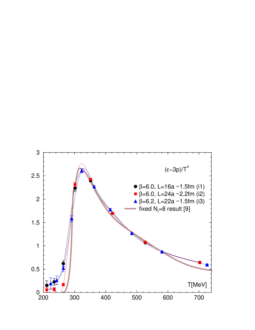
Figure 1: Trace anomaly on isotropic lattices as a function of physical temperature. The dotted lines are natural cubic spline interpolations. Horizontal errors due to the lattice scale are smaller than the symbols.

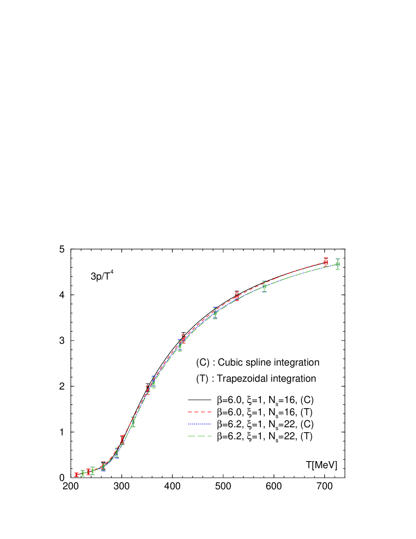
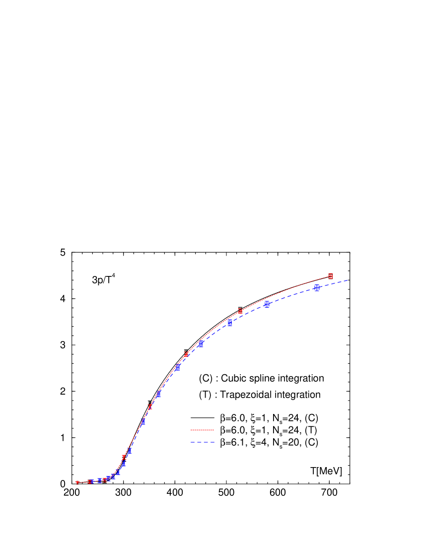
Figure 2: Comparison of the pressure using different interpolation functions for integration. Statistical errors are estimated by the jackknife method Okamoto:1999hi .

Our simulation parameters are listed in Table 1. On isotropic lattices, we calculate EOS on three lattices to study the volume and lattice spacing dependence. The ranges of $N_{t}$ correspond to $T=210$–700 MeV for the sets i1 and i2, and $T=220$–730 MeV for i3, respectively. The critical temperature corresponds to $N_{t}\sim 7$-8 for i1 and i2 and $\sim 10$ for i3, assuming $T_{c}\sim 290$ MeV in quenched QCD with the Sommer scale $r_{0}=0.5$ fm. The set a2 will be discussed in the next section. The zero temperature subtraction is performed with $N_{t}=16$ for i1 and i2, and with $N_{t}=22$ for i3. We generate up to a few millions configurations using the pseudo-heat-bath algorithm. Statistical errors are estimated by the jackknife analysis. Typically, bin size of a few thousands configurations are necessary near $T_{c}$, while a few hundreds are sufficient off the transition region.

Figure 1 shows $(\epsilon-3p)/T^{4}$. Dotted lines in the figure are the natural cubic spline interpolations. For comparison, we also reproduce the result of the fixed $N_{t}$ method at $N_{t}=8$ and $N_{s}=32$ Boyd:1996bx , for which we have rescaled the horizontal axis by $T_{c}=290$ MeV according to our choice of $r_{0}=0.5$ fm. At and below $T_{c}$, lattice size dependence is visible among the sets i1 ($L\approx 1.5$ fm), i2 (2.2 fm) and the fixed $N_{t}=8$ result (2.7 fm). On the other hand, the lattice spacing dependence is negligible between i1 ($a\approx 0.093$ fm) and i3 (0.068 fm). At higher $T$, $(\epsilon-3p)/T^{4}$ on our three lattices show good agreement, however they slightly deviate from the fixed $N_{t}$ one at $T>600$ MeV, presumably due to the coarseness of our lattices at these temperatures.

The integration of (2) is performed numerically using the natural cubic spline interpolations shown in Fig. 1. For the initial temperature $T_{0}$ of the integration, we linearly extrapolate the $(\epsilon-3p)/T^{4}$ data at a few lowest $T$’s because the values of $(\epsilon-3p)/T^{4}$ at our lowest $T$ are not exactly zero. In this study, we commonly take $T_{0}=150$ MeV as the initial temperature which satisfies $(\epsilon-3p)/T^{4}=0$, and estimate the integration from $T_{0}$ to the lowest $T$ by the area of the triangle.

We estimate the statistical error for the $T$-integration by the jackknife analysis at each $T$ and accumulate the contributions from different $T$’s by the error propagation Okamoto:1999hi , because simulations at different $N_{t}$ are statistically independent. Note that the error for the lattice scale do not affect the dimensionless quantity $p/T^{4}$. Error bars shown in the figures represent the statistical errors.

To estimate the systematic error due to the interpolation ansatz, we compare the results of $p/T^{4}$ using cubic spline interpolation and those with the trapezoidal rule in Fig. 2. (The results on the anisotropic $\xi=4$ lattice will be discussed later.) We find that the size of systematic errors due to the interpolation ansatz are comparable to that of the statistical ones. In Fig. 3, we note that the natural cubic spline interpolation curve of $(\epsilon-3p)/T^{4}$ for the set i2 shows small negative values at $T\approx 250$ MeV due to the nearby sharp edge at $T\approx 260$ MeV. From a comparison with the results of trapezoidal interpolation for that range, we find that the effect of this bump on the value of $p/T^{4}$ at $T>250$ MeV is 0.032. Although a negative pressure is unphysical, because this shift in $p/T^{4}$ is smaller than the statistical errors, we disregard the effects of the negative pressure in this paper. To avoid arbitrary data handlings, we just adopt the results of natural cubic spline interpolations as the central values in the followings.

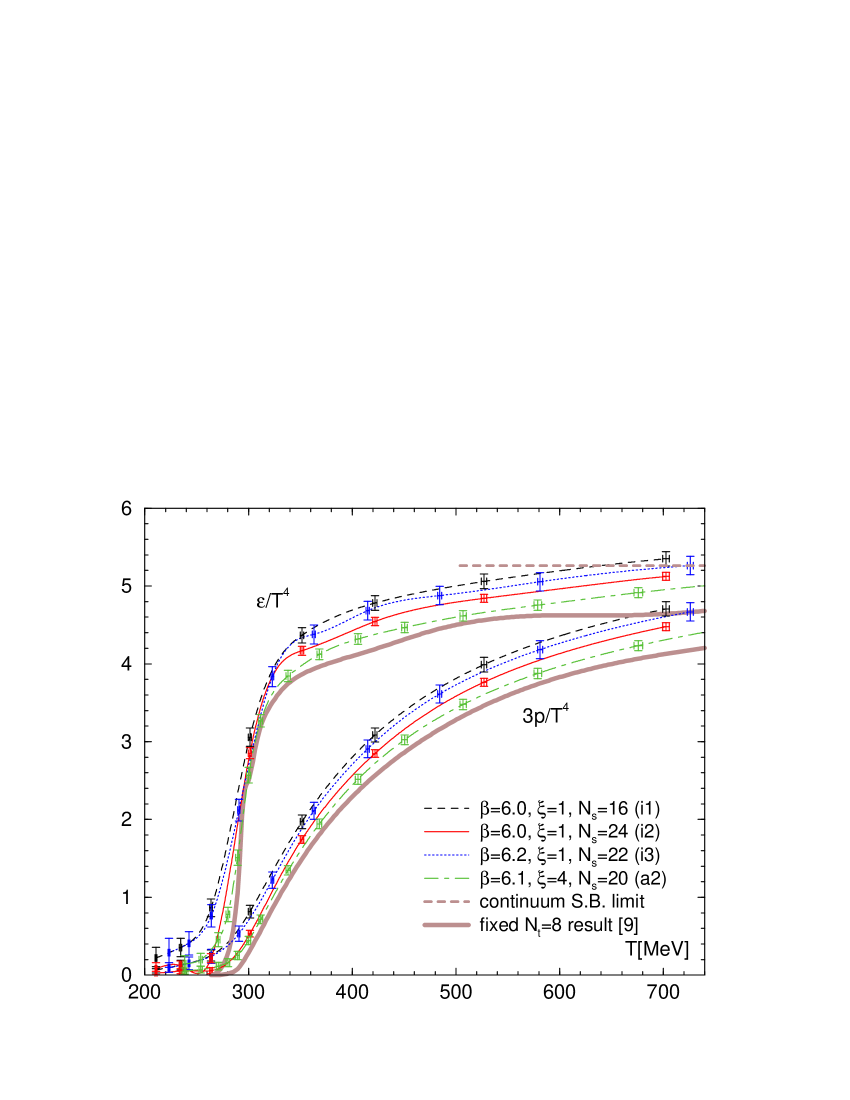
Figure 3: EOS on isotropic and anisotropic lattices. Dashed horizontal line represents the free gas case in the continuum (Stefan-Boltzmann limit).

In Fig. 3, we summarize the results of EOS. Results on the anisotropic lattice (a2) will be discussed later. The normalized energy density $\epsilon/T^{4}$ is calculated by combining $p/T^{4}$ and $(\epsilon-3p)/T^{4}$.

We find that, except for the vicinity of $T_{c}$, the EOS is rather insensitive to the variation of lattice size (between $L\approx 1.5$ fm and $2.2$ fm) and the lattice spacing (between $a\approx 0.093$ fm and 0.063 fm). The results of EOS agree within 10% for our variation of lattice parameters. This is in part due to the fact that $(\epsilon-3p)/T^{4}$ is not so sensitive to the lattice parameters up to high temperatures. Note also that, because $(\epsilon-3p)/T^{4}=0$ in the high temperature limit, the increasingly large lattice artifacts at large $T$ are naturally suppressed in the $T$-integration. Looking at the $T$ $>$$\sim$ $T_{c}$ region closer, we note a slight tendency that both $p$ and $\epsilon$ decrease as the lattice size (lattice spacing) becomes larger (smaller).

Near and below $T_{c}$, we observe a sizable finite size effect between $L\approx 1.5$ fm (i1) and $2.2$ fm (i2), while the effect of the lattice spacing is quite small (i1 and i3). Therefore, for a reliable simulation, we need, at least, $L$ $>$$\sim$ 2 fm.

Our results are qualitatively consistent with the previous EOS by the fixed $N_{t}$ method Boyd:1996bx . Quantitatively our results are slightly above the fixed $N_{t}$ results. The discrepancy can be in part understood by smaller spatial volumes below $T_{c}$ and the small values of $N_{t}$ at higher $T$ in our method.

IV EOS on anisotropic lattice

The anisotropic lattice with the temporal lattice finer than the spatial one is expected to improve the resolution of $T$ without much increasing the computational cost. To further test the systematic error due to the resolution of $T$, we perform the study with the $T$-integral method on an anisotropic lattice with the renormalized anisotropy $\xi=4$.

The simulation parameters are given as the set a2 in Table 1, which are the same as those adopted in Matsufuru:2001cp . We vary $N_{t}=34$–8 corresponding to $T=240$–1010 MeV. The zero temperature subtraction is performed with $N_{t}=80$. ($=20\times\xi$). We generate up to a few millions configurations.

We calculate the beta function $a_{s}(\partial\beta/\partial a_{s})_{\xi}$ by fitting the $r_{0}/a_{s}$ data Matsufuru:2001cp ; mapple with the Allton’s ansatz Allton:1996dn .

$$a_{s}/r_{0}=R(\beta)\cdot A\left(1+B\hat{f}^{2}(\beta)+C\hat{f}^{4}(\beta)\right),$$ (8)

where

$$R(\beta) = \left(\frac{6b_{0}}{\beta}\right)^{\!-b_{1}/(2b_{0}^{2})}\exp{\left(-\,\frac{\beta}{12b_{0}}\right)},$$

$$\hat{f}(\beta) = R(\beta)/R(6.10),\;\;b_{0}=\frac{11}{16\pi^{2}},\;\;b_{1}=\frac{102}{(16\pi^{2})^{2}}.$$

The best fit is achieved by $A=76.0(1.5)$, $B=0.190(32)$, and $C=0.0204(87)$ with $\chi^{2}/{\rm dof}=12.6/6$. The beta function is now obtained by

$$a_{s}\left(\frac{\partial\beta}{\partial a_{s}}\right)_{\!\!\xi}=\frac{12b_{0}^{2}\beta}{6b_{1}-b_{0}\beta}\,\frac{1+B\hat{f}^{2}+C\hat{f}^{4}}{1+3B\hat{f}^{2}+5C\hat{f}^{4}},$$ (9)

and its value at our simulation point is given in Table 1. For $(\partial\xi_{0}/\partial\beta)_{\xi}$ we adopt the result of Klassen:1998ua .

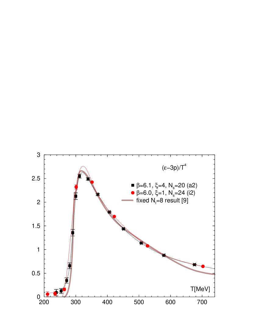
Figure 4: Trace anomaly on isotropic and anisotropic lattices with similar spatial lattice spacing and lattice size. The dotted lines are natural cubic spline interpolations.

In Fig. 4, we compare the trace anomaly obtained on the anisotropic lattice with that on the isotropic lattice with similar $a_{s}$ and $L$ (the set i2). We find that the results are generally consistent with each other, while, due to the cruder resolution in $T$, the natural cubic spline interpolation for the i2 lattice slightly overshoots the data on the a2 lattice around the peak at $T\approx 320$ MeV. We note that the height of the peak on the a2 lattice is similar to that of the fine i3 lattice shown in Fig. 1 and the fixed $N_{t}=8$ result. Similar to the case of the isotropic lattice, our result slightly overshoots the fixed $N_{t}$ result below $T_{c}$ and at $T>600$ MeV. Around the sharp lower edge at $T\approx 250$ MeV, the undershooting of the natural cubic spline interpolation on the i2 lattice, discussed in the previous section, is avoided by the finer data points on the a2 lattice.

The results of pressure on the a2 and i2 lattices are compared in the lower panel of Fig. 2. While they are roughly consistent with each other, we find that the pressure on the anisotropic lattice is slightly smaller than that on the isotropic lattice. This is in part due to the smaller values of $\epsilon-3p$ around the peak at $T\approx 320$ MeV. We also note a slight tendency that the trace anomaly on the a2 lattice is systematically lower than that on the i2 lattice by about $1\sigma$ in the high temperature side.

When we consider the difference between the a2 and i2 lattices as the systematic error due to the cruder $T$-resolution of the i2 lattice, the systematic error is about 2-3 times larger than the estimation in the previous section from a comparison of different interpolation ansätze. Therefore, for an estimation of the systematic error on isotropic lattices, it may be safer to assume a few times larger errors than those estimated from a comparison of different interpolation ansätze.

Some part of this difference in the EOS between a2 and i2 lattices might be explained by the difference of the lattice spacing in the temporal direction, since lattice artifacts of thermodynamic quantities generally have dominant contributions from the temporal lattice spacing Namekawa:2001 . Indeed this interpretation is supplemented by the fact that the difference in the EOS between i1 and i3 has a similar tendency as shown in Fig.3. We reserve further investigation of this possibility for future study.

V Conclusions

We proposed a fixed scale approach to investigate finite temperature QCD on the lattice. To calculate EOS non-perturbatively at fixed scale, we introduced the $T$-integral formula (2), in which $p$ is calculated as an integration of the trace anomaly $\epsilon-3p$ with respect to $T$. The fixed scale approach with the $T$-integral method enables us to efficiently utilize the results of previous $T=0$ spectrum studies. At intermediate and low temperatures, we can largely reduce the lattice artifacts than the fixed $N_{t}$ approach. On the other hand, our approach is not suitable for studying the approach to the high $T$ limit because of small $N_{t}$ there. Also, around and below $T_{c}$, the large values of $N_{t}$ may require high statistics due to large cancellations by the $T=0$ subtraction.

To test the $T$-integral method, we performed a series of simulations of SU(3) gauge theory on isotropic and anisotropic lattices. We found that the method works quite well. Our results of EOS for the quenched QCD on isotropic and anisotropic lattices are summarized in Fig. 3, which are qualitatively consistent with the previous results using the conventional fixed $N_{t}$ approach.

Our EOS in the high temperature region turned out to be roughly independent of the lattice spacing, lattice volume, and the anisotropy. All the results agree within about 10% for the range of our lattice parameters. With small statistical errors of less than about 2%, we identified small systematic shifts under the variations of lattice parameters. The smallness of them will be useful for precise continuum extrapolations. Around the critical temperature, we found that the lattice size should be at least larger than about 2 fm.

The fixed scale approach with the $T$-integral method is applicable to QCD with dynamical quarks too. With dynamical quarks, it is more convenient to simulate isotropic lattices, because the tuning of anisotropy parameters as well as the determination of the factors $\partial\xi_{0}/\partial\beta$ in (7) requires quite a few works for full QCD. Therefore, it is important to estimate the systematic error in EOS due to the limited resolution of $T$ on an isotropic lattice. From the test of quenched QCD presented in this paper, we found that this systematic error is under control and its order of magnitude can be correctly estimated by a comparison of different interpolation ansätze, though it may be safer to introduce a factor of about 2-3 to the estimates.

We are currently investigating EOS in $2+1$ flavor QCD with non-perturbatively improved Wilson quarks, using the configurations by the CP-PACS/JLQCD Collaboration nf2p1-wilson , which are public on the ILDG ILDG . The pseudo-critical temperature ($\sim 175$ MeV) is around $N_{t}\sim 16$ on the finest lattice with $a\approx 0.07$ fm. We are further planning to extend the study to use the $2+1$ flavor configurations by the PACS-CS Collaboration generated just at the physical values of the light quark masses PACS-CS .

TU thanks H. Matsufuru for helpful discussions and $r_{0}/a_{s}$ data on the anisotropic lattice. The simulations have been performed on supercomputers at RCNP, Osaka University and YITP, Kyoto University. This work is in part supported by Grants-in-Aid of the Japanese Ministry of Education, Culture, Sports, Science and Technology (Nos. 17340066, 18540253, 19549001, and 20340047). SE is supported by U.S. Department of Energy (DE-AC02-98CH10886).

References

- (1) T. Hirano, N. van der Kolk and A. Bilandzic, arXiv:0808.2684 [nucl-th].
- (2) C. DeTar, plenary talk at LATTICE 2008, to be published in PoS (LAT08) 042 (2008).
- (3) J. Engels, J. Fingberg, F. Karsch, D. Miller and M. Weber, Phys. Lett. B 252, 625 (1990).
- (4) A. Ali Khan et al. [CP-PACS collaboration], Phys. Rev. D 64, 074510 (2001) [arXiv:hep-lat/0103028].
- (5) J. Engels, F. Karsch, H. Satz and I. Montvay, Phys. Lett. B 101, 89 (1981).
- (6) L. Levkova, T. Manke and R. Mawhinney, Phys. Rev. D 73, 074504 (2006) [arXiv:hep-lat/0603031].
- (7) T. Yoshié, plenary talk at LATTICE 2008, to be published in PoS (LAT08) 042 (2008).
- (8) R. G. Edwards, U. M. Heller and T. R. Klassen, Nucl. Phys. B 517, 377 (1998) [arXiv:hep-lat/9711003].
- (9) G. Boyd et al., Nucl. Phys. B 469, 419 (1996) [arXiv:hep-lat/9602007].
- (10) H. Matsufuru, T. Onogi and T. Umeda, Phys. Rev. D 64, 114503 (2001) [arXiv:hep-lat/0107001].
- (11) M. Okamoto et al. [CP-PACS Collaboration], Phys. Rev. D 60, 094510 (1999) [arXiv:hep-lat/9905005].
- (12) H. Matsufuru, private communication.
- (13) C. R. Allton, Nucl. Phys. Proc. Suppl. 53, 867 (1997) [arXiv:hep-lat/9610014].
- (14) T. R. Klassen, Nucl. Phys. B 533, 557 (1998) [arXiv:hep-lat/9803010].
- (15) Y. Namekawa et al. [CP-PACS Collaboration], Phys. Rev. D 64, 074507 (2001) [arXiv:hep-lat/0105012].
- (16) T. Ishikawa et al. [CP-PACS/JLQCD Collaborations], Phys. Rev. D 78 , 011502(R) (2008) [arXiv:hep-lat/0704.1937].
- (17) Y. Kuramashi, plenary talk at LATTICE 2008, to be published in PoS (LAT08) 042 (2008).