Spectrum Sharing between Wireless Networks

Abstract

We consider the problem of two wireless networks operating on the same (presumably unlicensed) frequency band. Pairs within a given network cooperate to schedule transmissions, but between networks there is competition for spectrum. To make the problem tractable, we assume transmissions are scheduled according to a random access protocol where each network chooses an access probability for its users. A game between the two networks is defined. We characterize the Nash Equilibrium behavior of the system. Three regimes are identified; one in which both networks simultaneously schedule all transmissions; one in which the denser network schedules all transmissions and the sparser only schedules a fraction; and one in which both networks schedule only a fraction of their transmissions. The regime of operation depends on the pathloss exponent $\alpha$, the latter regime being desirable, but attainable only for $\alpha>4$. This suggests that in certain environments, rival wireless networks may end up naturally cooperating. To substantiate our analytical results, we simulate a system where networks iteratively optimize their access probabilities in a greedy manner. We also discuss a distributed scheduling protocol that employs carrier sensing, and demonstrate via simulations, that again a near cooperative equilibrium exists for sufficiently large $\alpha$.

1 Introduction

The recent proliferation of networks operating on unlicensed bands, most notably 802.11 and Bluetooth, has stimulated research into the study of how different systems competing for the same spectrum interact. Communication on unlicensed spectrum is desirable essentially because it is free, but users are subject to random interference generated by the transmissions of other users. Most research to date has assumed devices have no natural incentive to cooperate with one another. For instance, a wireless router in one apartment is not concerned about the interference it generates in a neighboring apartment. Following from this assumption, various game-theoretic formulations have been used to model the interplay between neighboring systems [16], [4], [1], [5], [12]. An important conclusion stemming from this body of work is that for single-stage games the Nash Equilibria (N.E.) are typically unfavorable, resulting in inefficient allocations of resources to users. A quintessential example is the following. Consider a system where a pair of competing links is subjected to white-noise and all cross-gains are frequency-flat. Suppose the transmitters wish to select a one-time power allocation across frequency subject to a constraint on the total power expended (this problem is studied in [15], [2], [3] where it is referred to as the Gaussian Interference Game). It is straightforward to reason (via a waterfilling argument) that the selection by both users of frequency-flat power allocations, each occupying the entire band, constitutes a N.E.. This full spread power allocation can be extremely inefficient. Consider a symmetric system where the cross-gains and direct-gains are equal. At high $\sf SNR$ each link achieves a throughput of only 1 b/s/Hz, instead of $\frac{1}{2}\log_{2}(1+\sf SNR)$ b/s/Hz, which would be obtained if the links cooperated by occupying orthogonal halves of the spectrum. At an $\sf SNR$ of 30 dB, the throughput ratio between cooperative behavior and this full spread N.E. behavior, referred to as the price of anarchy, is about 5. This example highlights an important point in relation to single-stage games between competing wireless links: users typically have an incentive to occupy all of the available resources.

In this work a different approach is taken. Rather than assuming total anarchy, that is, competition between all wireless links, we instead assume competition only between wireless links belonging to different networks. Wireless links belonging to the same network are assumed to cooperate. In short, we assume competition on the network level, not on the link level. In a practical setting this may represent the fact that neighboring wireless systems are produced by the same manufacturer, or are administered by the same network operator. Alternatively one may view the competition as being between coalitions of users [13].

To make the problem analytically tractable but still retain its underlying mechanics, we assume each network operates under a random-access protocol, where users from a given network access the channel independently but with the same probability. Analysis of random access protocols provides intuition for the behavior of systems operating under more complex protocols, as the access probability can broadly be interpreted as the average degrees of freedom each user occupies. For the case of competition on the link level, game-theoretic research of random-access protocols such as ALOHA have been conducted in [14] and [11]. In our model each network has a different density of nodes and chooses its access probability to maximize average throughput per user. Note this access protocol is essentially identical to one in which users select a random fraction of the spectrum on which to communicate. Thus an access probability of one corresponds to a full spread power allocation.

We first assume all links in the system have the same transmission range and afterwards show that the results are only trivially modified if each link is assumed to have an i.i.d. random transmission range. We characterize the N.E. of this system for a fixed-rate model, where all users transmit at the same data rate. We show that unlike the case of competing links, a N.E. always exists and is unique. Furthermore for a large range of typical parameter values, the N.E. is not full spread —nodes in at least one network occupy only a fraction of the bandwidth. We also identify two modes, delineated by the pathloss exponent $\alpha$. For $\alpha>4$, the N.E. behavior is distinctly different than for $\alpha<4$ and possesses pseudo-cooperative properties. Following this we show that the picture for the variable-rate model, in which users individually tailor their transmission rates to match the instantaneous channel capacity, remains unchanged. Before concluding we present simulation results for the behavior of the system when the networks employ a greedy algorithm to optimize their throughput, operating under both a random access protocol, and a carrier sensing protocol.

In section II we formulate the system model explicitly. In section III.A we introduce the random access protocol and analyze its N.E. behavior in the fixed-rate model. In section III.B we analyze the variable-rate model. In section IV we extend our results to cover the case of variable transmission ranges. Section V presents simulation results and the carrier sensing protocol. Section VI summarizes and suggests extensions. Section VII contains proofs of the main theorems presented.

2 Problem Setup

Consider two wireless networks consisting of $n\lambda_{1}$ and $n\lambda_{2}$ tx-rx pairs, respectively. Without loss of generality we will assume $\lambda_{1}\leq\lambda_{2}$. The transmitting nodes are uniformly distributed at random in an area of size $n$. To avoid boundary effects suppose this area is the surface of a sphere. Thus $\lambda_{i}$ is the density of transmitters (or receivers) in network $i$. For each transmitter, the corresponding receiver is initially assumed to be located at a fixed range of $d$ meters with uniform random bearing. Time is slotted and all users are assumed to be time synchronized.

Both networks operate on the same band of (presumably unlicensed) spectrum and at each time slot a subset of tx-rx pairs are simultaneously scheduled in each network. When scheduled a tx-rx pair uses all of the spectrum. It is generally desirable to schedule neighboring tx-rx pairs in different time slots. This scheduling model is a form of TDM, but is more or less analogous to an FDM model where each tx-rx pair is allocated a subset of the spectrum (typically overlapping in some way with other tx-rx pairs in the network).

Transmitting nodes are full buffer in that they always have data to send. Transmissions are assumed to use Gaussian codebooks and interference from other nodes is treated as noise. Initially we analyse the model where all transmissions in network $i$ occur at a common rate of $\log(1+\beta_{i})$. We refer to $\beta$ as the target $\sf SINR$. Thus a transmission in network $i$ is successful iff ${\sf SINR}>\beta_{i}$. Later we explore the model where transmission rates are individually tailored to match the instantaneous capacities of the channels. The signal power attenuates according to a power law with pathloss exponent $\alpha>2$. We assume a high-$\sf SNR$ or interference limited scenario where the thermal noise is insignificant relative to the received power of interfering nodes and thus refer to the $\sf SIR$ as the $\sf SIR$. For a given realization of the node locations the time-averaged throughput achieved by the $j$th tx-rx pair in network $i$ is then

$${\overline{R}}_{j}=f_{j}\mathbb{P}({\sf SIR_{j}(t)}>\beta_{i})\log(1+\beta_{i})$$

per complex d.o.f., where $f_{j}$ is the fraction of time the $j$th tx-rx pair is scheduled. The average (represented by the bar above the $R$) is essentially taken over the distribution of the interference as at different times different subsets of transmitters are scheduled.

As for $\alpha>2$ the bulk of the interference is generated by the strongest interferer, to make the problem tractable, we compute the $\sf SIR$ as the receive power of the desired signal divided by the receive power of the nearest interferers signal. We refer to this as the Dominant Interferer assumption. Denote the range of the nearest interferer to the $j$th receiver at time $t$ by $r_{j}(t)$. Then

$${\sf SIR}_{j}(t)=\frac{d^{-\alpha}}{r_{j}^{-\alpha}(t)}$$

The metric of interest to each network is its expected time-averaged rate per user,

$${\mathbb{E}}{\overline{R}}={\mathbb{E}}_{g}\left[f_{j}\mathbb{P}({\sf SIR_{j}(t)}>\beta_{i})\log(1+\beta_{i})\right]$$

The subscript $g$ indicates this expectation is taken over the geographic distribution of the nodes. As the setup is statistically symmetric, this metric is equivalent to the expected sum rate of the system, divided by $n\lambda_{i}$, in the limit $n\rightarrow\infty$.

3 Random Access protocol

3.1 Fixed-Rate model

Suppose each network uses the following random access protocol. At each time slot each link is scheduled i.i.d. with probability $p_{i}$. The packet size is $\log(1+\beta_{i})$ for all communications in network $i$. The variables $\beta_{i}$ are optimized over.

Let us first compute the optimal access probability for the case of a single network operating in isolation on a licensed band, as a function of the node density and the transmission range. This problem has recently been studied independently in [6]-[9] with equivalent results derived. In [10] similar results are derived for the case where the $\sf SIR$ is computed based on all interferers, not just the nearest.

Let the r.v. $N_{j}(x)$ denote the number of interfering transmitters within range $x$ of the $j$th receiver.

$${\mathbb{E}}{\overline{R}} ={\mathbb{E}}_{g}\left[f_{j}\mathbb{P}(r_{j}(t)>\beta_{i}^{1/\alpha}d)\log(1+\beta_{I})\right]$$

$$=p_{i}\sum_{k=1}^{n\lambda_{i}-1}{\mathbb{P}}(N_{j}(\beta^{1/\alpha}d)=k)(1-p_{i})^{k}\log(1+\beta_{i})$$

$$=p_{i}\sum_{k=1}^{n\lambda_{i}-1}\left(\frac{\pi\beta_{i}^{2/\alpha}d^{2}}{n}\right)^{k}\left(1-\frac{\pi\beta_{i}^{2/\alpha}d^{2}}{n}\right)^{n\lambda_{i}-k-1}$$

$$\quad\quad\quad\quad\quad\times\binom{n\lambda_{i}-1}{k}(1-p_{i})^{k}\log(1+\beta_{i})$$

$$=p_{i}\left(1-p_{i}\frac{\pi\beta_{i}^{2/\alpha}d^{2}}{n}\right)^{n\lambda_{i}-1}\log(1+\beta_{i})$$

$$\rightarrow p_{i}\log(1+\beta_{i})e^{-\pi\lambda_{i}d^{2}p_{i}\beta_{i}^{2/\alpha}}$$

in the limit $n\rightarrow\infty$.

In order to obtain better insight into the problem at hand, a change of variables is required. We refer to the set of all points within the transmission range as the transmission disc. The quantity $\pi\lambda_{i}d^{2}$ is the average number of nodes (tx or rx) per transmission disc. We often refer to it simply as the number of nodes per disc and represent it by the symbol

$$N_{i}\triangleq\pi\lambda_{i}d^{2}.$$

Assume $N_{i}$ is larger than a certain threshold (we make this precise later). Maximizing over the access probability yields

$${\mathbb{E}}{\overline{R}}\rightarrow\frac{\log(1+\beta_{i})}{N_{i}\beta_{i}^{2/\alpha}}e^{-1}$$ (1)

with the optimal access probability being

$$p_{i}^{*}=\frac{1}{N_{i}\beta_{i}^{2/\alpha}}.$$ (2)

One can further optimize over the target $\sf SIR$ so that $\beta_{i}$ is replaced by $\beta_{i}^{*}$ in the above two equations. Inspection of equation (1) reveals that the optimal target $\sf SIR$ is a function of $\alpha$ alone. So if we define the quantity

$$\Lambda_{i}\triangleq N_{i}p_{i},$$

$\Lambda_{i}^{*}$ will be a constant, independent of $N_{i}$. The quantity $\Lambda_{i}$ represents the average number of (simultaneous) transmissions per transmission disc. We sometimes refer to it simply as the transmit density. Whereas the domain of $p_{i}$ is $[0,1]$, the domain of $\Lambda_{i}$ is $[0,N_{i}]$. Thus we see that for $N_{i}$ sufficiently large, the access probability should be set such that an optimal number of transmissions per disc is achieved. What is this optimal number? What is the optimal target $\sf SIR$?

For the purposes of optimizing equation (1), define the function $\Lambda^{*}(\alpha)$ as the unique solution of the following equation

$$\frac{\alpha}{2}=\left(1+{\Lambda^{*}}^{\alpha/2}\right)\log\left(1+\frac{1}{{\Lambda^{*}}^{\alpha/2}}\right).$$ (3)

A plot of $\Lambda^{*}(\alpha)$ is given in figure 1. So as to avoid confusion, note that the symbol $\Lambda^{*}$ represents a pre-defined function, not necessarily the same as the symbol $\Lambda_{i}^{*}$, which is a variable. As equation (1) is smooth and continuous with a unique maxima, by setting it’s derivative to zero we find that the optimal target $\sf SIR$ is $\beta^{*}={\Lambda^{*}}^{-\alpha/2}$ and the optimal number of transmissions per disc is $\Lambda_{i}^{*}=\Lambda^{*}$, when $N_{i}$ is larger than a certain threshold.

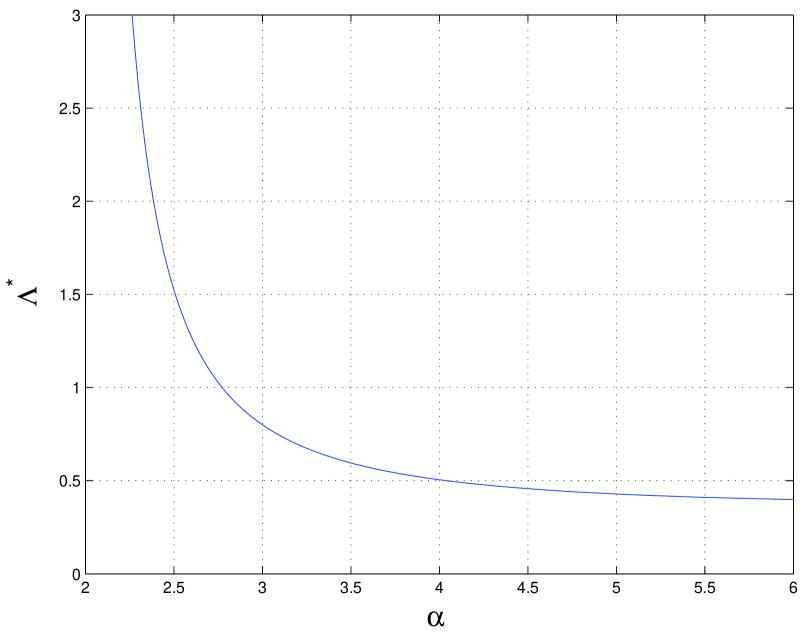
Figure 1: Optimal average number of transmissions per transmission disc as a function of the pathloss exponent.

When $N_{i}$ is smaller than this threshold, there aren’t enough tx-rx pairs to reach the optimal number of transmissions per disc, even when all of them are simultaneously scheduled. In this case the solution lies on the boundary with $p_{i}^{*}=1$. This corresponds to the scenario where the transmission range is short relative to the node density such that tx-rx pairs function as if in isolation. It is intuitive that in this case all transmissions in the network will be simultaneously scheduled. Our discussion is summarized in the following theorem.

Theorem 3.1.

(Optimal Access Probability) For a single network operating in isolation under the random access protocol, when $N_{i}>\Lambda^{*}$ the optimal access probability is $p_{i}^{*}=\frac{\Lambda^{*}}{N_{i}}$, where $\Lambda^{*}$ is given by the unique solution of equation (3). The optimal target $\sf SIR$ is $\beta_{i}^{*}={\Lambda^{*}}^{-\alpha/2}$.

When $N_{i}\leq\Lambda^{*}$, $p_{i}^{*}=1$ and $\beta_{i}^{*}$ is given by the unique solution to

$$\frac{\alpha}{2N_{i}{\beta_{i}^{*}}^{2/\alpha}}=\left(1+\frac{1}{\beta_{i}^{*}}\right)\log(1+\beta_{i}^{*}).$$

The region satisfying $N_{i}>\Lambda^{*}$ is referred to as the partial reuse regime. The complement region is referred to as the full reuse regime. Note the optimal access probability of the above theorem is equivalent to the results of section IV.B in [6], and those discussed under the title “Maximum Achievable Spatial Throughput and TC” on page 4137 of [8].

Now we perform the same computation for the case where both networks operate on the same unlicensed band. In this case there is both intra-network and inter-network interference. It is straightforward to extend the above analysis to show that for network $i$

$${\mathbb{E}}{\overline{R}}_{i}\rightarrow\frac{\Lambda_{i}}{N_{i}}\log(1+\beta_{i})e^{-(\Lambda_{1}+\Lambda_{2})\beta_{i}^{2/\alpha}}$$

in the limit $n\rightarrow\infty$. For a given $\Lambda_{2}$ the first network can optimize $\Lambda_{1}$ and $\beta_{1}$, and vice-versa. That is each network can iteratively adjust its access probability and target $\sf SIR$ in response to the other networks. In this sense a game can be defined between the two networks. A strategy for network $i$ is a choice of $\Lambda_{i}\in[0,N_{i}]$ and $\beta_{i}>0$. Its payoff function (also referred to as utility function) is the limiting form of ${\mathbb{E}}{\overline{R}}_{i}$ times $N_{i}$,

$$U_{1}\left((\Lambda_{1},\beta_{1}),(\Lambda_{2},\beta_{2})\right) =\Lambda_{1}\log(1+\beta_{1})e^{-(\Lambda_{1}+\Lambda_{2})\beta_{1}^{2/\alpha}}$$ (4)

$$U_{2}\left((\Lambda_{1},\beta_{1}),(\Lambda_{2},\beta_{2})\right) =\Lambda_{2}\log(1+\beta_{2})e^{-(\Lambda_{1}+\Lambda_{2})\beta_{2}^{2/\alpha}}.$$ (5)

Here we have scaled the throughput by $N_{i}$ to emphasize the simple form of the payoff functions. At first glance this setup seems desirable but there is a redundancy in the way the strategy space has been defined. The problem is that the variable $\beta_{i}$ only appears in $U_{i}$ and thus should be optimized over separately rather than being included as part of the strategy. This leads to the following game setup.

Definition 3.2.

(Random Access Game) A strategy for network $i$ in the Random Access Game is a choice of $\Lambda_{i}\in[0,N_{i}]$. The payoff functions are

$$U_{1}(\Lambda_{1},\Lambda_{2}) =\max_{\beta_{1}>0}\Lambda_{1}\log(1+\beta_{1})e^{-(\Lambda_{1}+\Lambda_{2})\beta_{1}^{2/\alpha}}$$

$$U_{2}(\Lambda_{1},\Lambda_{2}) =\max_{\beta_{2}>0}\Lambda_{2}\log(1+\beta_{2})e^{-(\Lambda_{1}+\Lambda_{2})\beta_{2}^{2/\alpha}}.$$

The above formulation is intuitively appealing as a networks choice of access probability constitutes its entire strategy. If we could explicitly solve the maximization problems, the variables $\beta_{i}$ would be removed altogether. When $\Lambda_{1}$ and $\Lambda_{2}$ are large this can be done and

$$U_{1}(\Lambda_{1},\Lambda_{2}) \approx\frac{\Lambda_{1}}{(\Lambda_{1}+\Lambda_{2})^{\alpha/2}}\cdot(\alpha/2)^{\alpha/2}e^{-\alpha/2}$$ (6)

$$U_{2}(\Lambda_{1},\Lambda_{2}) \approx\frac{\Lambda_{2}}{(\Lambda_{1}+\Lambda_{2})^{\alpha/2}}\cdot(\alpha/2)^{\alpha/2}e^{-\alpha/2},$$ (7)

but in general it is not possible. Instead, since we are only interested in analyzing the Nash equilibrium (N.E.) or equilibria of this game, we do the following.

Observe that the objective function within the maximization is smooth and continuous. This enables the order of maximization to be swapped. That is, for a given $\Lambda_{2}$, we first maximize over $\Lambda_{1}$ in equation (4) and then over the $\beta_{1}$. Likewise for equation (5). The benefit of this approach is that the maximizing $\Lambda_{i}$ can be explicitly expressed as a function of $\beta_{i}$. This was demonstrated earlier for the single network scenario. The resulting expressions are

$$U_{1}(\Lambda_{1},\Lambda_{2})$$

$$=\left\{\begin{array}[]{ll}\Lambda_{1}\log\left(1+\Lambda_{1}^{-\alpha/2}\right)e^{-\Lambda_{2}/\Lambda_{1}-1},&\hbox{$\Lambda_{1}<N_{1}$;}\\ \max_{\beta_{1}>0}\log(1+\beta_{1})e^{-(N_{1}+\Lambda_{2})\beta_{1}^{2/\alpha}},&\hbox{$\Lambda_{1}=N_{1}$.}\end{array}\right.$$

$$U_{2}(\Lambda_{1},\Lambda_{2})$$

$$=\left\{\begin{array}[]{ll}\Lambda_{2}\log\left(1+\Lambda_{2}^{-\alpha/2}\right)e^{-\Lambda_{1}/\Lambda_{2}-1},&\hbox{$\Lambda_{2}<N_{2}$;}\\ \max_{\beta_{2}>0}\log(1+\beta_{2})e^{-(N_{2}+\Lambda_{1})\beta_{2}^{2/\alpha}},&\hbox{$\Lambda_{2}=N_{2}$.}\end{array}\right.$$

The set of N.E. of the above game and their corresponding values of $U_{1}$ and $U_{2}$ are identical to those of the Random Access Game. Inspection of the above equations reveals a further simplification of the problem is at hand —the set of N.E. of the above game are identical to the set of N.E. of the following game (though the values of $U_{1}$ and $U_{2}$ at the equilibria may be different).

Definition 3.3.

(Transformed Random Access Game) A strategy for network $i$ in the Transformed Random Access Game is a choice of $\Lambda_{i}\in[0,N_{i}]$. The payoff functions are

$$U_{1}(\Lambda_{1},\Lambda_{2}) =\Lambda_{1}\log\left(1+\Lambda_{1}^{-\alpha/2}\right)e^{-\frac{\Lambda_{2}}{\Lambda_{1}}-1}$$

$$U_{2}(\Lambda_{1},\Lambda_{2}) =\Lambda_{2}\log\left(1+\Lambda_{2}^{-\alpha/2}\right)e^{-\frac{\Lambda_{1}}{\Lambda_{2}}-1},$$

We now analyze the N.E. of the Random Access Game by analyzing the N.E. of the Transformed Random Access Game. The first question of interest is whether or not there exists a N.E.? It turns out a unique N.E. always exists but its nature depends crucially on the pathloss exponent. There are two modes, $2<\alpha<4$ and $\alpha>4$. We start with the first.

Theorem 3.4.

(Random Access N.E. for $2<\alpha<4$) For $2<\alpha<4$ the unique N.E. occurs at $\Lambda_{1}^{*}=N_{1}$, and $\Lambda_{2}^{*}$ defined by either the solution of

$$N_{1}=\Lambda_{2}\left(\frac{\alpha}{2\left(1+{\Lambda_{2}}^{\alpha/2}\right)\log\left(1+{\Lambda_{2}}^{-\alpha/2}\right)}-1\right)$$ (8)

or $N_{1}$, whichever is smaller.

The N.E. described in theorem 3.4 occurs on the boundary of the strategy space. This is because for $2<\alpha<4$ each network tries to set its number of transmissions per disc higher than the other (see the proof of the theorem). The equilibrium is then only attained when at least one network has maxed out and scheduled all of its transmissions simultaneously.

The N.E. can be better understood when $N_{1}\gg 1$ corresponding to the case in which transmissions span several intermediate nodes.

Theorem 3.5.

(Random Access N.E. for $2<\alpha<4$ and $N_{1}\gg 1$) In the limit $N_{1}\rightarrow\infty$ the N.E. occurs at

$$(\Lambda_{1}^{*},\Lambda_{2}^{*})$$

$$\quad\quad=\left\{\begin{array}[]{ll}(N_{1},N_{2}),&\hbox{$N_{1}\leq N_{2}\leq\dfrac{2}{\alpha-2}N_{1}$}\\ \left(N_{1},\dfrac{2}{\alpha-2}N_{1}\right),&\hbox{$\dfrac{2}{\alpha-2}N_{1}\leq N_{2}$.}\end{array}\right.$$

This result stems from using the limiting form $\log(1+x)\rightarrow x$ as $x\rightarrow 0$ in the utility functions $U_{1}$ and $U_{2}$, as was done in equations (6) and (7). From it we see that if the denser network has more than $\approx 2/(\alpha-2)$ times as many nodes as its rival, the N.E. will correspond to partial reuse, i.e. the denser network will only occupy a fraction of the total available bandwidth. This is in stark contrast to the case of competing individual transmissions where the N.E. typically corresponds to a full spread, i.e. both competing links spread their power evenly across the entire bandwidth. The limit result of theorem LABEL:thm:apx_soln is plotted in figure 2 as a dashed line.

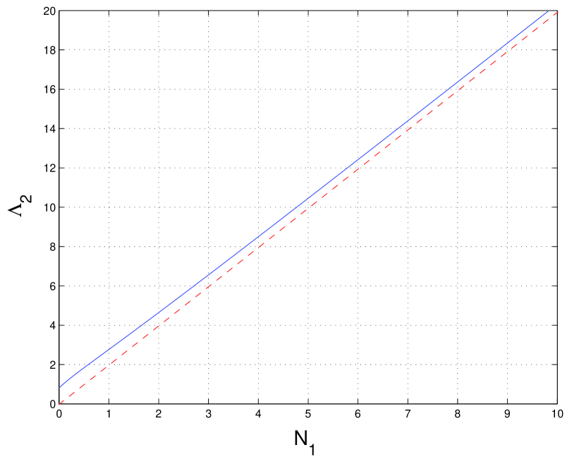
Figure 2: The solid line represents the solution to equation (8) for $\alpha=3$. The N.E. value $\Lambda_{2}^{*}$ is equal to the minimum of this line and $N_{2}$. The limiting solution used in theorem LABEL:thm:apx_soln is plotted as a dashed line.

We now investigate the average throughput at equilibrium for the mode $2<\alpha<4$. We define the metric

$$U_{e}=U_{1}(\Lambda_{1}^{*},\Lambda_{2}^{*})+U_{2}(\Lambda_{1}^{*},\Lambda_{2}^{*})$$

This quantity has a natural interpretation. Recall $\mathbb{E}{\overline{R}}_{i}$ is the average throughput per tx-rx pair and $N_{i}$ is the average number of tx-rx pairs per transmission disc in network $i$. Thus $U_{i}=N_{i}\mathbb{E}{\overline{R}}_{i}$ is the average throughput per transmission disc in network $i$. This is the average number of bits successfully received in network $i$ within an area of size $\pi d^{2}$ per time slot, per d.o.f.. The quantity $U_{e}$ is then the average throughput per transmission disc in the system, that is, the average number of bits successfully received in both networks within an area of size $\pi d^{2}$ per time slot, per d.o.f..

Theorem 3.6.

In the limit $N_{1}\rightarrow\infty$

$$U_{e}\rightarrow\left\{\begin{array}[]{ll}\dfrac{c_{1}(\alpha)}{N_{1}^{\alpha/2-1}}&\hbox{$N_{1}\leq N_{2}\leq\frac{2}{\alpha-2}N_{1}$}\\ \dfrac{c_{2}(\alpha)}{(N_{1}+N_{2})^{\alpha/2-1}},&\hbox{$\frac{2}{\alpha-2}N_{1}\leq N_{2}$.}\end{array}\right.$$

where $c_{1}(\alpha)=\left(\alpha/2-1\right)^{\alpha/2-1}(\alpha/2)e^{-\alpha/2}$ and $c_{2}(\alpha)=(\alpha/2)^{\alpha/2}e^{-\alpha/2}$.

The important property of this result is that as the number of nodes per transmission disc increases, $U_{e}$ decreases roughly like $1/(N_{1}+N_{2})^{\alpha/2-1}$. Let us compare this to the average throughput per transmission disc in the cooperative case, that is when the two networks behave as if they were a single network with $N_{1}+N_{2}$ nodes per disc. From equation (1) this average throughput per disc is

$$U_{c}=\Lambda^{*}\log(1+{\Lambda^{*}}^{-\alpha/2})$$

which is independent of the number of nodes per disc. Thus as the number of nodes per disc grows, so does the price of anarchy

$$\frac{U_{c}}{U_{e}}=O\left(N_{1}^{\alpha/2-1}\right).$$

For $\alpha>4$ the N.E. behavior is different. Whereas for $2<\alpha<4$ the solution always lies on the boundary, for $\alpha>4$ it typically does not.

Theorem 3.7.

(Random Access N.E. for $\alpha>4$) For $\alpha>4$ the unique N.E. occurs at

$$(\Lambda_{1}^{*},\Lambda_{2}^{*})=(\sqrt{\Lambda^{*}(\alpha/2)},\sqrt{\Lambda^{*}(\alpha/2)})$$

if $\sqrt{\Lambda^{*}(\alpha/2)}<N_{1}$, otherwise $\Lambda_{1}^{*}=N_{1}$ and $\Lambda_{2}^{*}$ is defined by either the solution of equation (8) or $N_{2}$, whichever is smaller.

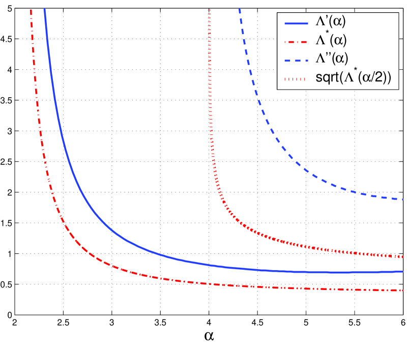
Figure 8: The functions $\Lambda^{\prime\prime}(\alpha)$ and $\Lambda^{\prime}(\alpha)$ for the Variable-Rate model versus the equivalent functions $\Lambda^{*}(\alpha)$ and $\sqrt{(}\Lambda^{*}(\alpha/2))$ for the Fixed-Rate model.

A plot of $\sqrt{\Lambda^{*}(\alpha/2)}$ versus $\alpha$ is given in figure 8. The condition $\sqrt{\Lambda^{*}(\alpha/2)}<N_{1}$ corresponds to network $1$ having more than $\sqrt{\Lambda^{*}(\alpha/2)}$ nodes per transmission disc. We refer to this as the partial/partial reuse regime.

The interpretation of theorem 3.7 is that for $\alpha>4$ in the partial/partial reuse regime, the solution lies in the strict interior of the strategy space. This is because on the boundary of the space network $i$ can improve its throughput by undercutting the transmit density of network $j$, i.e. setting $\Lambda_{i}<\Lambda_{j}$. The symmetry of the N.E. ($\Lambda_{1}^{*}=\Lambda_{2}^{*}$) then follows by observing the utility functions are symmetric and the solution is unique.

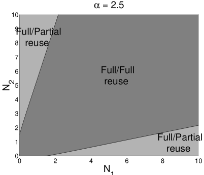
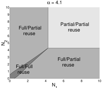
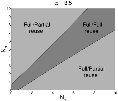
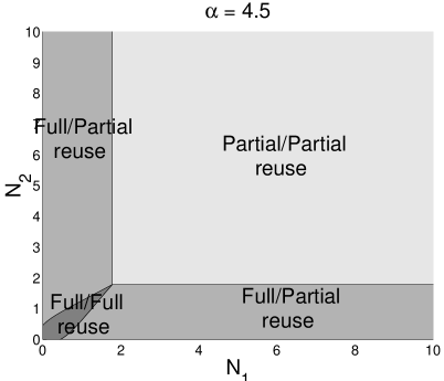
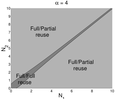
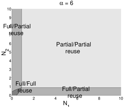
Figure 3: These plots can be used to determine which regime the N.E. is in. The x-axis and y-axis corresponds to the average number of nodes per transmission disc in network 1 and 2, respectively. Note the lower left vertex of the partial/partial reuse regime always occurs at $(\sqrt{\Lambda^{*}(\alpha)},\sqrt{\Lambda^{*}(\alpha)})$ and the intersection of the full/full reuse regime with the axes always occurs at $(\Lambda^{*}(\alpha),0)$ and $(0,\Lambda^{*}(\alpha))$.

There is a cooperative flavor to this equilibrium in that both networks set their transmission densities to the same level, and this level is comparable to the optimal single network density $\Lambda^{*}(\alpha)$. Moreover the equilibrium level does not grow with the number of nodes per transmission disc, as it does for $2<\alpha<4$. Actual cooperation between networks corresponds to setting the access probability based on equation (2), taking into account that the effective node density is $\lambda_{1}+\lambda_{2}$. Thus the cooperative solution is

$$(\Lambda_{1}^{*},\Lambda_{2}^{*})=\left(\frac{\lambda_{1}}{\lambda_{1}+\lambda_{2}}\Lambda^{*},\frac{\lambda_{2}}{\lambda_{1}+\lambda_{2}}\Lambda^{*}\right).$$

Under cooperation the average throughput per transmission disc is (from equation (1))

$$U_{c}=\frac{1}{e}\Lambda^{*}(\alpha)\log\left(1+\frac{1}{{\Lambda^{*}(\alpha)}^{\alpha/2}}\right).$$

Under cooperation in the partial/partial reuse regime it is

$$U_{e}=\frac{2}{e^{2}}\sqrt{\Lambda^{*}(\alpha/2)}\log\left(1+\frac{1}{{\Lambda^{*}(\alpha/2)}^{\alpha/4}}\right)$$

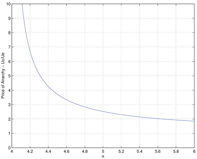
Figure 4: For $\alpha>4$, the price of anarchy depends only on the pathloss exponent in the partial/partial reuse regime.

The price of anarchy is the ratio of these two quantities ($U_{e}/U_{c}$) and is plotted in figure 4. Comparing the two modes we see that whereas for $2<\alpha<4$ the price of anarchy grows in an unbounded fashion with the number of nodes per transmission disc, for $\alpha>4$ the price of anarchy in the partial/partial reuse regime is a constant depending only on $\alpha$.

We now summarize the equilibria results. There are three regimes.

1. Full/Full reuse
   - $N_{1}\leq\sqrt{\Lambda^{*}(\alpha/2)}$ and $N_{1}\leq N_{2}\left(\alpha/2(1+{N_{2}}^{\alpha/2})\log(1+{N_{2}}^{-\alpha/2})-1\right)$
   - both networks schedule all transmissions

2. Full/Partial reuse
   - $N_{1}\leq\sqrt{\Lambda^{*}(\alpha/2)}$ and $N_{1}>N_{2}\left(\alpha/2(1+{N_{2}}^{\alpha/2})\log(1+{N_{2}}^{-\alpha/2})-1\right)$
   - denser network schedules all transmissions, sparser schedules only a fraction

3. Partial/Partial reuse
   - $N_{1}>\sqrt{\Lambda^{*}(\alpha/2)}$
   - both networks schedule only a fraction of their transmissions

In the full/full reuse regime $(\Lambda_{1}^{*},\Lambda_{2}^{*})=(N_{1},N_{2})$. In the full/partial reuse regime the sparser network sets $\Lambda_{1}^{*}=N_{1}$ and the denser network sets $\Lambda_{2}^{*}$ as the solution to equation (8). In the partial/partial reuse regime $(\Lambda_{1}^{*},\Lambda_{2}^{*})=(\sqrt{\Lambda^{*}(\alpha/2)},\sqrt{\Lambda^{*}(\alpha/2)})$.

The regimes are essentially distinguished by which boundary constraints are active. For $2<\alpha<4$ the partial/partial reuse regime is not accessible. Figure 3 provides an illustrated means for determining which regime the system is in, for a range of values of the pathloss exponent. In these plots we consider all values of $N_{1}$ and $N_{2}$, not just those satisfying $N_{1}\geq N_{2}$. Notice that as $\alpha\rightarrow 2$ the entire region corresponds to the full/full reuse regime, for $\alpha=4$ almost the entire region corresponds to the full/partial reuse regime and for $\alpha\rightarrow\infty$ the entire region corresponds to the partial/partial reuse regime.

3.2 Variable-Rate model

In this section we examine the case where tx-rx pairs tailor their communication rates to suit instantaneous channel conditions, sending at rate $\log(1+{\sf SIR(t)})$ during the $t$th time slot. Various protocols can be used to enable tx-rx pairs to estimate their ${\sf SIR}(t)$.

Consider first the single, isolated network scenario. The expected time-averaged rate per user is now

$$\mathbb{E}{\overline{R}}_{i}=p_{i}\mathbb{E}\log(1+{\sf SIR}).$$

As before, the rate is both time-averaged over the interference and averaged over the geographic distribution of the nodes. The $\sf SIR$ is the instantaneous value observed by a given rx node and is distributed according to

$$\mathbb{P}({\sf SIR}>x) =\mathbb{P}(r>x^{1/\alpha}d)$$

$$=\left(1-\frac{\pi x^{2/\alpha}d^{2}p_{i}}{n}\right)^{n\lambda_{i}}$$

where the variable $r$ denotes the distance to the nearest interferer. Thus

$$\mathbb{E}{\overline{R}}_{i} =p_{i}\int{\mathbb{P}}\left(\log(1+{\sf SINR})>s\right)ds$$

$$=p_{i}\int{\mathbb{P}}\left({\sf SINR}>x\right)\frac{dx}{1+x}$$

$$=p_{i}\int_{0}^{\left(\frac{n}{p_{i}\pi d^{2}}\right)^{\alpha/2}}\left(1-\frac{\pi x^{2/\alpha}d^{2}p_{i}}{n}\right)^{n\lambda_{i}}\frac{dx}{1+x}$$

$$\rightarrow p_{i}\int_{0}^{\infty}e^{-\pi p_{i}\lambda_{i}d^{2}x^{2/\alpha}}\frac{dx}{1+x}$$

in the limit $n\rightarrow\infty$. Changing variables and optimizing we have

$$\mathbb{E}{\overline{R}}_{i}\rightarrow\frac{1}{N_{i}}\max_{0\leq\Lambda_{i}\leq 1}\Lambda_{i}\int_{0}^{\infty}e^{-\Lambda_{i}x^{2/\alpha}}\frac{dx}{1+x}.$$ (9)

Define $\Lambda^{\prime}(\alpha)$ as the maximizing argument of the unconstrained version of the above optimization problem, or more specifically as the unique solution to

$$\int_{0}^{\infty}\frac{1-\Lambda^{\prime}x^{2/\alpha}}{1+x}e^{-\Lambda x^{2/\alpha}}dx=0.$$

The function $\Lambda^{\prime}(\alpha)$ is plotted in figure 8. Then

$$p_{i}^{*}=\min(\Lambda^{\prime}(\alpha)/N_{i},1)$$

From this we see that the solution for the variable-rate case is the same as the fixed-rate solution, differing only by substitution of the function $\Lambda^{\prime}(\alpha)$ for $\Lambda^{*}(\alpha)$.

Now we turn to the case of two competing wireless networks. Using an approach similar to the one above it can be shown that

$$\mathbb{E}{\overline{R}}_{i}\rightarrow\frac{1}{N_{i}}\Lambda_{i}\int_{0}^{\infty}e^{-(\Lambda_{1}+\Lambda_{2})x^{2/\alpha}}\frac{dx}{1+x}.$$

In this way we can define the game between the two networks like so.

Definition 3.8.

(Variable Rate Random Access Game) A strategy for network $i$ in the Variable Rate Random Access Game is a choice of $\Lambda_{i}\in[0,\pi\lambda_{i}d^{2}]$. The payoff functions are

$$U_{1}(\Lambda_{1},\Lambda_{2}) =\Lambda_{1}\int_{0}^{\infty}e^{-(\Lambda_{1}+\Lambda_{2})x^{2/\alpha}}\frac{dx}{1+x}$$

$$U_{2}(\Lambda_{1},\Lambda_{2}) =\Lambda_{2}\int_{0}^{\infty}e^{-(\Lambda_{1}+\Lambda_{2})x^{2/\alpha}}\frac{dx}{1+x}.$$

From the above definition we see that the Fixed-Rate game is derived from the Variable-Rate game by merely applying a step-function lower bound to the players utility functions, with the width of the step-function optimized, i.e.

$$\int_{0}^{\infty}e^{-(\Lambda_{1}+\Lambda_{2})x^{2/\alpha}}\frac{dx}{1+x}$$

$$\quad\quad\quad\quad\geq\max_{\beta_{i}>0}e^{-(\Lambda_{1}+\Lambda_{2})\beta_{i}^{2/\alpha}}\int_{0}^{\beta_{i}}\frac{dx}{1+x}$$

$$\quad\quad\quad\quad=\max_{\beta_{i}>0}\log(1+\beta_{i})e^{-(\Lambda_{1}+\Lambda_{2})\beta_{i}^{2/\alpha}}.$$

A plot comparing the expression on the left as a function of $\Lambda_{1}+\Lambda_{2}$, to the expression on the right as a function of $\Lambda_{1}+\Lambda_{2}$, for $\alpha=4$, is presented in figure 5. The figure suggests that both expressions share a similar functional dependency on $\Lambda_{1}+\Lambda_{2}$. It is therefore natural to wonder whether, as a consequence of this close relationship, the N.E. of the Variable-Rate game bears any relationship to the N.E. of the Fixed-Rate game?

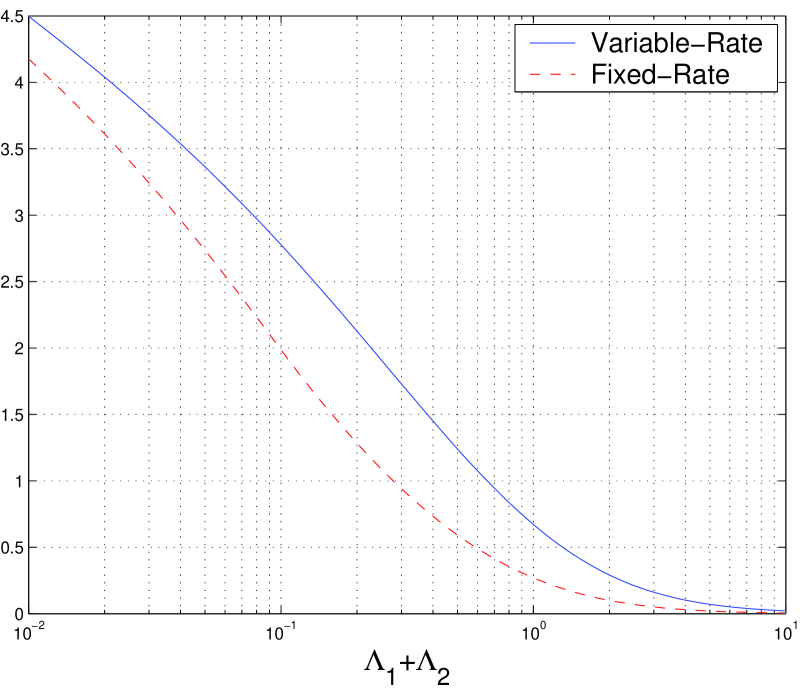
Figure 5: The utility functions used in the Fixed-Rate model are lower bounds of those used in the Variable-Rate model. In this sample plot $\alpha=4$. The y-axis represents $U_{i}/\Lambda_{i}$.

As in the Fixed-Rate game, the utility functions of the Variable-Rate game can be explicitly evaluated when $\Lambda_{1}$ and $\Lambda_{2}$ are large yielding

$$U_{1}(\Lambda_{1},\Lambda_{2}) \approx\frac{\Lambda_{1}}{(\Lambda_{1}+\Lambda_{2})^{\alpha/2}}\cdot\Gamma(\alpha/2+1)$$

$$U_{2}(\Lambda_{1},\Lambda_{2}) \approx\frac{\Lambda_{2}}{(\Lambda_{1}+\Lambda_{2})^{\alpha/2}}\cdot\Gamma(\alpha/2+1).$$

Comparing with equations (4) and (5) we see that for large $\Lambda_{1},\Lambda_{2}$, the utility functions of the Variable-Rate game have exactly the same functional dependency on $\Lambda_{1},\Lambda_{2}$ as the utility functions of the Fixed-Rate game, differing only in an $\alpha$-dependent constant. These constants are plotted in figure 6. The plots illustrate the benefit in total system throughput that stems from playing the Variable-rate game in place of the Fixed-Rate game.

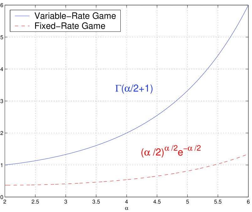
Figure 6: The total system throughputs at equilibrium for the Variable-Rate and Fixed-Rate games differ only by $\alpha$-dependent constants. These constants are plotted above. For the Variable-Rate game the constant is $\Gamma(\alpha/2+1)$ versus $(\alpha/2)^{\alpha/2}e^{-\alpha/2}$ for the Fixed-Rate game.

As anticipated by the above discussion, the N.E. behavior of the Variable-Rate game parallels that of the Fixed-Rate game. The same two modes are present, $2<\alpha<4$ and $\alpha>4$. These give rise to the same three spreading regimes, the only difference being that the boundaries delineating them are shifted slightly. The N.E. values $(\Lambda_{1}^{*},\Lambda_{2}^{*})$ in each regime take on a similar form.

Theorem 3.9.

The Variable-Rate Random Access Game has a unique N.E. $(\Lambda_{1}^{*},\Lambda_{2}^{*})$ which lies in one of three regions. Let $\Lambda^{\prime\prime}(\alpha)$ be the unique solution of

$$\int_{0}^{\infty}\frac{1-\Lambda^{\prime\prime}x^{2/\alpha}}{1+x}e^{-2\Lambda^{\prime\prime}x^{2/\alpha}}dx=0.$$ (10)

for $\alpha>4$, and equal to positive infinity for $\alpha\leq 4$.

• (Full/Full reuse) If $N_{1}\leq\Lambda^{\prime\prime}(\alpha)$ and $N_{2}\leq$ the unique solution over $\Lambda$ of

  $$\int_{0}^{\infty}\frac{1-\Lambda x^{2/\alpha}}{1+x}e^{-(N_{1}+\Lambda)x^{2/\alpha}}dx=0,$$ (11)

  then $(\Lambda_{1}^{*},\Lambda_{2}^{*})=(N_{1},N_{2})$.

• (Full/Partial reuse) If $N_{1}\leq\Lambda^{\prime\prime}(\alpha)$ and $N_{2}>$ the unique solution of equation (11) then $\Lambda_{1}^{*}=1$ and $\Lambda_{2}^{*}$ is equal to this unique solution.

• (Partial/Partial reuse) If $N_{1}>\Lambda^{\prime\prime}(\alpha)$ then $(\Lambda_{1}^{*},\Lambda_{2}^{*})=(\Lambda^{\prime\prime}(\alpha),\Lambda^{\prime\prime}(\alpha))$.

A regime map is provided in figure 7. As is evident from the above theorem, it is not possible to characterize the behavior of the N.E. for the Variable-Rate game as explicitly as for the Fixed-Rate game. This is in part due to the more complex representation of the utility functions in terms of integrals, and in part due to the fact that the the function $\Lambda^{\prime\prime}(\alpha)$ cannot be represented in terms of the function $\Lambda^{\prime}(\alpha)$, as in the case of the Fixed-Rate game, where one function equals the square-root of the other evaluated at $\alpha/2$.

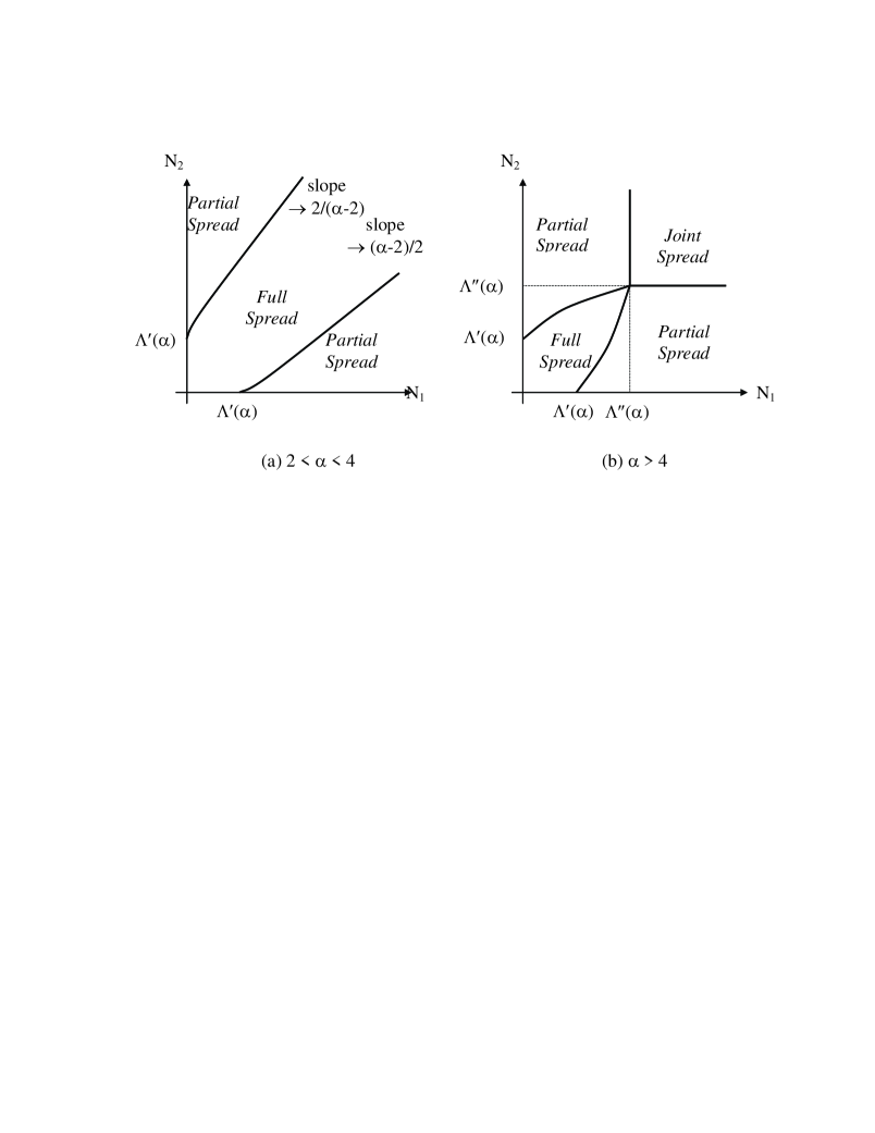
Figure 7: The three regimes for the N.E. of the Variable-Rate Game.

For large $N_{1}$ however, we can use the approximation adopted in theorem LABEL:thm:apx_soln to explicitly characterize the behavior of the N.E. in the full/partial reuse regime.

Theorem 3.10.

(Variable-Rate Random Access N.E. for $2<\alpha<4$ and $N_{1}\gg 1$) In the limit $N_{1}\rightarrow\infty$ the N.E. occurs at

$$(\Lambda_{1}^{*},\Lambda_{2}^{*})$$

$$\quad\quad=\left\{\begin{array}[]{ll}(N_{1},N_{2}),&\hbox{$N_{1}\leq N_{2}\leq\dfrac{2}{\alpha-2}N_{1}$}\\ \left(N_{1},\dfrac{2}{\alpha-2}N_{1}\right),&\hbox{$\dfrac{2}{\alpha-2}N_{1}\leq N_{2}$.}\end{array}\right.$$

Thus for $2<\alpha<4$ and large $N_{1}$, the behavior of the N.E. in the Variable-Rate game is identical to that of the Fixed-Rate game. As discussed earlier, the values of $U_{1}$ and $U_{2}$ at equilibrium are equal to those of the Fixed-Rate game times a constant $(\alpha/2)^{\alpha/2}e^{-\alpha/2}/\Gamma(\alpha/2+1)$.

3.3 Explanation of Behavior

The intuition behind our result is the following. The average throughput per link is essentially equal to the product of the fraction of time transmissions are scheduled, and the average number of bits successfully communicated per transmission. Adjusting the transmit density has a linear effect on the former term, but a non-linear effect on the latter. The latter depends on the $\sf SIR$ and the $\sf SIR$ essentially depends on the pathloss exponent via

$${\sf SIR}\approx\left(\frac{\text{distance to transmitter}}{\text{distance to interferer}}\right)^{\alpha}$$

When the nearest interferer is closer than the transmitter, the ratio inside the parentheses is less than one, and a large value of $\alpha$ substantially hurts the $\sf SIR$, dragging it to near zero and causing the link capacity to drop to near zero. However, when the nearest interferer is further away than the transmitter, the ratio is greater than one and a large value of $\alpha$ substantially improves the $\sf SIR$, resulting in a large link capacity. Thus for large $\alpha$ the average number of bits successfully communicated per transmission is very sensitive to whether or not the transmission disc is empty.

This insensitivity for sufficiently small $\alpha$ means that increasing the transmit density in network $i$ causes a linear increase in the fraction of time transmissions are scheduled, but has little effect on the number of bits successfully communicated per transmission, up until the point where the transmit density of network $i$ starts to dwarf the transmit density of network $j$. Thus network $i$ will wish to increase its transmit density until it is sufficiently larger than network $j$’s. Likewise network $j$ will wish to increase its transmit density until it is sufficiently larger than network $i$’s. Ultimately this results in either

1. a full/full reuse solution, which occurs when the sparser network max’s out and winds up simultaneously scheduling all of its transmissions, and the denser network is insufficiently dense such that its optimal transmit density based on the sparser networks choice, results in it simultaneously scheduling all of its transmissions, or

2. a full/partial reuse solution, which occurs when the sparser network max’s out and winds up simultaneously scheduling all of its transmissions but the denser network is sufficiently dense such that its optimal transmit density based on the sparser networks choice, results in it simultaneously scheduling only a fraction of its transmissions.

The opposite effect occurs for sufficiently large $\alpha$, where the average number of bits successfully communicated per transmission depends critically on whether or not there is an interferer inside the transmission disc. In this scenario network $i$ will set its active density to a level lower than network $j$’s, in order to capitalize on those instances in which network $j$ happens to not schedule any transmissions nearby to one of network $i$’s receivers, resulting in the successful communication of a large number of bits. Likewise network $j$ will set its active density to a level lower than network $i$’s, and the system converges to the partial/partial reuse regime.

4 Variable Transmission Range

One of our initial assumptions was that all tx-rx pairs have the same transmission range $d$. In this section we consider the scenario where the transmission ranges of all tx-rx pairs in the system are i.i.d. random variables $D_{j}$. When the variance of $D_{j}$ is large, some form of power control may be required to ensure long range transmissions are not unfairly penalized. A natural form of power control involves tx nodes setting their transmit powers such that all transmissions are received at the same $\sf SNR$. This means transmit power scales proportional to $D_{j}^{\alpha}$. Denote the distance from the $k$th tx node to the $j$th rx node $D_{ij}$. Then the interference power from the $k$th tx node impinging on the $j$th rx node is proportional to $D_{kk}^{\alpha}/D_{kj}^{\alpha}$. In the fixed transmission range scenario this quantity was proportional to $1/D_{kj}^{\alpha}$. There we assumed the bulk of the interference was generated by the dominant interferer. Denote the scheduled set of tx nodes at time $t$ by ${\cal A}(t)$. This assumption essentially evoked the following approximation

$$\sum_{k\in\cal A(t)}1/D_{kj}(t)^{\alpha}\approx\max_{k\in\cal A(t)}1/D_{kj}(t)^{\alpha}.$$

The equivalent approximation for the variable transmission range problem is

$$\sum_{k\in\cal A(t)}D_{kk}^{\alpha}/D_{kj}(t)^{\alpha}\approx\max_{k\in\cal A(t)}D_{kk}^{\alpha}/D_{kj}(t)^{\alpha}.$$

Thus for variable range transmission the dominant interferer is not necessarily the nearest to the receiver. Under this assumption the $\sf SIR$ at the $j$th rx node at time $t$ is then

$${\sf SIR}_{j}(t)=\frac{D_{k^{*}k^{*}}^{-\alpha}}{D_{k^{*}j^{*}}^{-\alpha}}$$

where $k^{*}$ is the index of the tx node that is closest to the $j$th receiver relative to its transmission range.

Let us compute the throughput for the variable transmission range model under the Fixed-Rate Random Access protocol.

$${\mathbb{E}}{\overline{R}}=p_{i}{\mathbb{P}}\left({\sf SIR}_{j}(t)>\beta_{i}\right)\log(1+\beta_{i}).$$

The probability the $\sf SIR$ is greater than the threshold

$${\mathbb{P}}({\sf SINR_{j}(t)>\beta_{i}}) ={\mathbb{P}}\left(D_{kj}>\beta_{i}^{1/\alpha}D_{kk},\forall k\right)$$

$$=\left(\int_{0}^{\sqrt{n/\pi}/\beta_{i}^{1/\alpha}}{\mathbb{P}}\left(D_{kj}>\beta_{i}^{1/\alpha}x\right){\mathbb{P}}_{D_{kk}}(x)dx\right)^{n\lambda}$$

$$=\left(\int_{0}^{\sqrt{n/\pi}/\beta_{i}^{1/\alpha}}\left(1-\frac{p_{i}\pi\beta_{i}^{2/\alpha}x^{2}}{n}\right){\mathbb{P}}_{D_{kk}}(x)dx\right)^{n\lambda}$$

$$=\left(1-\frac{p_{i}\pi\beta_{i}^{2/\alpha}}{n}\int_{0}^{\sqrt{n/\pi}/\beta_{i}^{1/\alpha}}x^{2}{\mathbb{P}}_{D_{kk}}(x)dx\right)^{n\lambda}$$

$$=\left(1-\frac{p_{i}\pi\beta_{i}^{2/\alpha}{\mathbb{E}}D_{kk}^{2}}{n}\right)^{n\lambda}$$

$$\rightarrow e^{-p_{i}\pi\beta_{i}^{2/\alpha}{\mathbb{E}}D_{kk}^{2}}$$

as $n\rightarrow\infty$. For notational simplicity let $d\equiv D_{kk}$. If we define $N_{i}$ as the average number of nodes per transmission disc, where the average is taken over both the geographical distribution of the nodes and the distribution of the size of the transmission disc, i.e.

$$N_{i}=\pi\lambda_{i}{\mathbb{E}}_{d}^{2}$$

we wind up with ${\mathbb{E}}{\overline{R}}\rightarrow p_{i}\log(1+\beta_{i})e^{-N_{i}p_{i}\beta_{i}^{2/\alpha}}$, which is the same result as the fixed-transmission range model. It is straightforward to extend the analysis to the case of two competing networks. The throughput per user in network 1 is then

$${\mathbb{E}}{\overline{R}}\rightarrow p_{1}\log(1+\beta_{1})e^{-(N_{1}p_{1}+N_{2}p_{2})\beta_{1}^{2/\alpha}}.$$

Likewise for network 2. From this we see that all results for the fixed-transmission range model extend to the variable-transmission range model by simply replacing $d^{2}$ by ${\mathbb{E}}d^{2}$.

5 Simulations

5.1 Random Access Protocol

In order to get a sense of the typical behavior of the players in the (Variable-Rate) Random Access game, and to justify the validity of the Dominant Interferer assumption, we simulate the behavior of the following greedy algorithm with the interference computed based on all transmissions in the network, not just the strongest.

Inputs: $p_{1}(0),p_{2}(0),\Delta$
Outputs: ${\bf p}_{i}=[p_{i}(1),\dots,p_{i}(500)]$, for $i=1,2$.

For $t=1$ to $500$

Form estimate $\overline{R}_{1}(p_{1}(t-1)+\Delta,p_{2}(t-1))$

Form estimate $\overline{R}_{1}(p_{1}(t-1)-\Delta,p_{2}(t-1))$

If $\overline{R}_{1}(p_{1}(t-1)+\Delta,p_{2}(t-1))>\overline{R}_{1}(p_{1}(t-1)-\Delta,p_{2}(t-1))$

$p_{1}(t)=\min(p_{1}(t-1)+\Delta,1)$

Else

$p_{1}(t)=\max(p_{1}(t-1)-\Delta,0)$

End

Form estimate $\overline{R}_{2}(p_{1}(t),p_{2}(t-1)+\Delta)$

Form estimate $\overline{R}_{2}(p_{1}(t),p_{2}(t-1)-\Delta)$

If $\overline{R}_{2}(p_{1}(t),p_{2}(t-1)+\Delta)>\overline{R}_{2}(p_{1}(t),p_{2}(t-1)-\Delta)$

$p_{2}(t)=\min(p_{2}(t-1)+\Delta,1)$

Else

$p_{2}(t)=\max(p_{2}(t-1)-\Delta,0)$

End

End

Each update time $t$, network 1 temporarily sets its access probability to $p_{1}(t-1)+\Delta$ and measures the resulting throughput, averaged over 200 transmission times. This is denoted $\overline{R}_{1}(p_{1}(t-1)+\Delta,p_{2}(t-1))$. It then repeats this measurement for an access probability of $p_{1}(t-1)-\Delta$. This is denoted $\overline{R}_{1}(p_{1}(t-1)-\Delta,p_{2}(t-1))$. It then either permanently increases its access probability to $p_{1}(t)=p_{1}(t-1)+\Delta$ or permanently decreases it to $p_{1}(t)=p_{1}(t-1)-\Delta$ depending on which option it estimates will lead to a higher throughput. Now network 2 performs the same operation. It uses a total of 400 time slots to measure the effect of increasing versus decresing its access probability and then either sets $p_{2}(t)=p_{2}(t-1)+\Delta$ or $p_{2}(t)=p_{2}(t-1)-\Delta$. If $\Delta$ is small, then both networks can perform these measurement operations simultaneously without significantly affecting the outcome.

The topology used in the simulations consisted of 400 tx nodes from network 1 and 200 tx nodes from network 2, all i.i.d. uniformly distributed in a square of unit area. For each tx node, its corresponding rx node was located at a point randomly chosen at uniform from a disc of radius 0.15. This corresponds to $N_{1}=400/\sqrt{(}800)\approx 14.14$ and $N_{2}=200/\sqrt{(}800)\approx 7.28$. A step-size of $\Delta=0.02$ was used. When computing the throughputs, in order to avoid boundary effects, only transmissions emanating from those tx nodes in the interior of the network were counted. The results for $\alpha=2.5,3.5$ and $4.5$ are displayed in figure 9. The observed behavior corresponds to the analytical results. For the values of $N_{1}$ and $N_{2}$ used, the N.E. lies in the Full/Full regime for $\alpha=2.5$, the Full/Partial regime for $\alpha=3.5$, and the Partial/Partial regime for $\alpha=4.5$, as can be seen from figure 3.

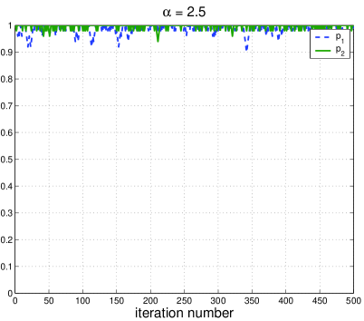
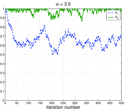
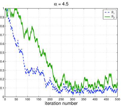
Figure 9: Simulations of greedy algorithm under Random Access protocol.

5.2 Carrier Sensing Multiple Access based protocol

The high level conclusion from our analysis of the Random Access protocol, is that the Nash Equilibrium is cooperative in nature for a sufficiently high pathloss exponent. Ideally we would like to be able to draw this conclusion for a more sophisticated class of scheduling protocols employing carrier sensing. Due to the analytical intractability of the problem, we present simulation results to illustrate this effect. We assume both networks operate under the following protocol. We present a centralized version of it due to space constraints, but claim there exists a distributed version that performs identically in most cases. During the scheduling phase, each tx-rx pair is assigned a unique token at random from $\{1,\dots,n\}$. Tx nodes proceed with their transmission so long as they will not cause excessive interference to any rx node with a higher priority token. More precisely, a transmission is scheduled so long as for each rx node with higher priority, the difference between its received signal power in dB and the interference power from the lower priority tx node in dB, exceeds a silencing threshold $\gamma_{i}$ ($i=1$ for network 1 and $i=2$ for network 2). Thus a game between the two networks can be defined where the strategies are the choices of silencing thresholds $\gamma_{1}$ and $\gamma_{2}$. We refer to this as the CSMA game. The silencing threshold for the CSMA game essentially plays the same role as the access probability in the Random Access game -it determines the degree of spatial reuse. A high value of $\gamma$ leads to a low density of transmissions, a low value of $\gamma$ leads to a high density.

We simulate the behavior that arises when both networks optimize their silencing thresholds in a greedy manner. Analogously to before, we have the following algorithm.

Inputs: $p_{1}(0),p_{2}(0),\Delta$
Ouputs: ${\bf p}_{i}=[p_{i}(1),\dots,p_{i}(500)]$, for $i=1,2$.

For $t=1$ to $500$

Form estimate $\overline{R}_{1}(\gamma_{1}(t-1)+\Delta,\gamma_{2}(t-1))$

Form estimate $\overline{R}_{1}(\gamma_{1}(t-1)-\Delta,\gamma_{2}(t-1))$

If $\overline{R}_{1}(\gamma_{1}(t-1)+\Delta,\gamma_{2}(t-1))>\overline{R}_{1}(\gamma_{1}(t-1)-\Delta,\gamma_{2}(t-1))$

$\gamma_{1}(t)=\min(\gamma_{1}(t-1)+\Delta,30{\sf dB})$

Else

$\gamma_{1}(t)=\max(\gamma_{1}(t-1)-\Delta,-30{\sf dB})$

End

Form estimate $\overline{R}_{2}(\gamma_{1}(t),\gamma_{2}(t-1)+\Delta)$

Form estimate $\overline{R}_{2}(\gamma_{1}(t),\gamma_{2}(t-1)-\Delta)$

If $\overline{R}_{2}(\gamma_{1}(t),\gamma_{2}(t-1)+\Delta)>\overline{R}_{2}(\gamma_{1}(t),\gamma_{2}(t-1)-\Delta)$

$\gamma_{2}(t)=\min(\gamma_{2}(t-1)+\Delta,30{\sf dB})$

Else

$\gamma_{2}(t)=\max(\gamma_{2}(t-1)-\Delta,-30{\sf dB})$

End

End

The topology used in the setup is identical to before, the only exception being that at each iteration of the algorithm, 10 old tx-rx pairs leave each network, and 10 new pairs join in i.i.d. locations drawn uniformly at random. This is to ensure sufficient averaging.

In a similar fashion to before, each network estimates the effect of either increasing or decreasing the silencing threshold and then makes a permanent choice. For the same parameter values, the results of the simulation are displayed in figure 10. On the y-axes of these plots we have drawn the fraction of nodes simultaneously scheduled at each iteration, which we denote $f_{1}$ and $f_{2}$, rather than the silencing thresholds $\gamma_{i}$, in order to draw a simple visual comparison with figure 9. For this reason there is more fluctuation in the results, as the fraction of simultaneously scheduled transmissions varies not only due to the up/down movements of the silencing thresholds, but also due to the changing topology.

We conclude from these plots that for small values of $\alpha$ (namely $\alpha=2.5$) the system converges to a competitive equilibrium, where both networks simultaneously schedule a large fraction of their transmissions, and for large values of $\alpha$ (namely $\alpha=3.5$ and $4.5$) the system converges to a near cooperative equilibrium, where both networks schedule a small fraction of their transmissions.

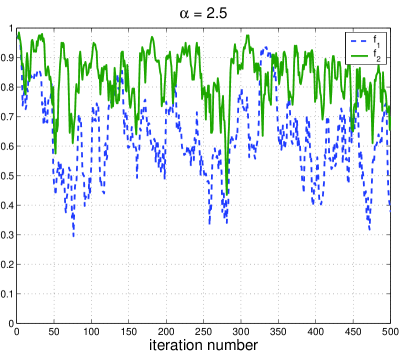
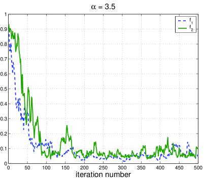
Figure 10: Simulations of greedy algorithm under Carrier Sensing Multiple Access protocol

6 Conclusion

This work studied spectrum sharing between wireless devices operating under a random access protocol. The crucial assumption made was that nodes belonging to the same network or coalition cooperate with one another. Competition only exists between nodes belonging to rival networks. It was found that cooperation between devices within each network created the necessary incentive to prevent total anarchy. For pathloss exponents greater than four, we showed that contrary to ones intuition, there can be a natural incentive for devices to cooperate to the extent that each occupies only a fraction of the available bandwidth. Such results are optimistic and encouraging. We demonstrated via simulations that it may be possible to extend them to more complex operating protocols such as those that employ carrier-sensing to determine when the medium is free. More generally one wonders whether a multi-stage game capturing the system dynamics under such a protocol can be formulated, and whether the desirable properties of the single-stage game continue to hold. It would also be worthwhile investigating the incentives wireless links have to form coalitions, as in this work it was in essence assumed that coalitions had been pre-determined.

7 Proofs

7.1 Theorem 3.1

The limiting expression for the average throughput is

$${\mathbb{E}}{\overline{R}}(p_{i},\beta_{i})\rightarrow p_{i}\log(1+\beta_{i})e^{-N_{i}p_{i}\beta_{i}^{2/\alpha}}.$$

Given a $\beta_{i}$ there is a single maximum over $p_{i}$. By differentiation we have

$$\frac{\partial{\mathbb{E}}{\overline{R}}}{\partial{p_{i}}}=\left(1-p_{i}N_{i}\beta_{i}^{2/\alpha}\right)\log(1+\beta_{i})e^{-N_{i}p_{i}\beta_{i}^{2/\alpha}},$$

so $p_{i}^{*}=\min(1,1/N_{i}\beta_{i}^{2/\alpha})$. Thus

$${\mathbb{E}}{\overline{R}}(p_{i}^{*},\beta_{i})=\left\{\begin{array}[]{ll}\log(1+\beta_{i})e^{-N_{i}\beta_{i}^{2/\alpha}},&\hbox{$\beta_{i}\leq N_{i}^{-2/\alpha}$},\\ \dfrac{\log(1+\beta_{i})e^{-1}}{N_{i}\beta_{i}^{2/\alpha}},&\hbox{$\beta_{i}>N_{i}^{-2/\alpha}$}.\end{array}\right.$$

Both of these functions have one maximum, but the maximum of the second function is always greater than the maximum of the first as it represents the solution to the unconstrained problem

$$\max_{p_{i}>0,\beta_{i}>0}{\mathbb{E}}{\overline{R}}(p_{i},\beta_{i}),$$

whereas the maximum of the first represents the solution to

$$\max_{p_{i}=1,\beta_{i}>0}{\mathbb{E}}{\overline{R}}(p_{i},\beta_{i}).$$

Thus if the maximum of the second function occurs for $\beta_{i}>N_{i}^{-2/\alpha}$, it is the maximum of the entire function, but if it occurs for $\beta_{i}\leq N^{-2/\alpha}$, the maximum of the entire function is the maximum of the first function over the domain $\beta_{i}\leq N^{-2/\alpha}$. By differentiation we find the maximum of the second function occurs at the unique solution of

$$\frac{\alpha}{2}=(1+1/\beta_{i})\log(1+\beta_{i})$$

which is $\beta_{i}={\Lambda^{*}}^{-\alpha/2}$. Thus if $N_{i}>\Lambda^{*}$, the solution is $p^{*}=\Lambda^{*}/N_{i}$ and $\beta_{i}^{*}={\Lambda^{*}}^{-\alpha/2}$. If $N_{i}\leq\Lambda^{*}$ the solution is $p^{*}=1$ and $\beta_{i}^{*}$ equal to the unique solution of

$$\frac{\alpha}{2N_{i}\beta_{i}^{2/\alpha}}=(1+1/\beta_{i})\log(1+\beta_{i})$$ (12)

or $N_{i}^{-2/\alpha}$, whichever is smaller. But as $(1+1/x)\log(1+x)$ is a monotonically increasing function, from the definition of $\Lambda^{*}$ we have

$$\frac{\alpha}{2}\leq\left(1+N_{i}^{\alpha/2}\right)\log\left(1+N_{i}^{-\alpha/2}\right)$$

whenever $N_{i}\leq\Lambda^{*}$. Combining this with equation (12) and using the monotonicity of $(1+1/x)\log(1+x)$ we see that the unique solution to equation (12) is always smaller than $N_{i}^{-2/\alpha}$. This establishes the desired result.

7.2 Theorem 3.4

First we show that any N.E. must lie on the boundary of the strategy space, i.e. $\Lambda_{i}=1$ for some $i$. The utility functions are smooth and continuous. Differentiating $U_{1}$ with respect to $\Lambda_{1}$ yields

$$\frac{\partial U_{1}}{\partial\Lambda_{1}}=e^{-\Lambda_{2}/\Lambda_{1}}\left(\frac{\Lambda_{2}}{\Lambda_{1}}-\frac{\alpha}{2\left(1+\Lambda_{1}^{\alpha/2}\right)\log\left(1+\Lambda_{1}^{-\alpha/2}\right)}+1\right)$$

Consider the function $f(x)=(1+x)\log(1+1/x)$. As $f(x)$ is monotonically decreasing for $x\geq 0$ and $\lim_{x\rightarrow\infty}f(x)=1$ we have $f(x)>1$ for all $x\geq 0$. Thus for $\alpha<4$, ${\partial U_{1}}/{\partial\Lambda_{1}}>0$ whenever $\Lambda_{1}<\Lambda_{2}$ and similarly ${\partial U_{2}}/{\partial\Lambda_{2}}>0$ whenever $\Lambda_{2}<\Lambda_{1}$. Thus for a N.E. to occur in the interior of the strategy space we must have both $\Lambda_{1}>\Lambda_{2}$ and $\Lambda_{2}>\Lambda_{1}$. As these conditions are mutually exclusive at least one of the constraints of the strategy space must be active at the N.E.. In essence each network is trying to set it’s active density higher than the other’s. Eventually at least one network maxs out.

First consider the case where the solution to

$$N_{1}=x\left(\frac{\alpha}{2\left(1+{x}^{\alpha/2}\right)\log\left(1+{x}^{-\alpha/2}\right)}-1\right).$$ (13)

occurs for $x<N_{2}$. Suppose $\Lambda_{2}^{*}=N_{2}$. Then as $N_{1}\leq N_{2}$ we have $\Lambda_{1}\leq\Lambda_{2}^{*}$, hence $\partial U_{1}/\partial\Lambda_{1}>0$ for all $\Lambda_{1}$ on the interior and hence $\Lambda_{1}^{*}=N_{1}$. Now the function $U_{2}(\Lambda_{1}^{*},\Lambda_{2})$ has a unique maximum for $\Lambda_{2}$. This maximum satisfies $\partial U_{2}(\Lambda_{1}^{*},\Lambda_{2})\partial\Lambda_{2}=0$, which is equation (13) with $\Lambda_{2}^{*}$ substituted for $x$. But the solution equation (13) satisfies $x<N_{2}$, so $\Lambda_{2}^{*}<N_{2}$, a contradiction. Thus the constraint $\Lambda_{2}\leq N_{2}$ must be inactive. Suppose instead that the constraint $\Lambda_{1}^{*}=N_{1}$ is active. Then by the same arguments the unique $\Lambda_{2}^{*}$ satisfies equation (13). This establishes the solution and it’s uniqueness, for the first case.

Second consider the case where the solution to equation (13) occurs for $x\geq N_{2}$. Then it is straightforward to check using similar arguments above, that the unique solution satisfies $(\Lambda_{1}^{*},\Lambda_{2}^{*})=(N_{1},N_{2})$. This establishes the result.

7.3 Theorem 3.5

For $\alpha>2$ the solution to equation (8) only goes to infinity for $N_{1}\rightarrow\infty$. In this limit $(1+{\Lambda_{2}^{*}}^{\alpha/2})\log(1+{\Lambda_{2}^{*}}^{-\alpha/2})\rightarrow 1$ and

$$\Lambda_{2}^{*}\rightarrow\frac{2}{\alpha-2}\Lambda_{1}^{*}$$

if $N_{1}\leq(\alpha/2-1)N_{2}$. Otherwise, $\Lambda_{2}^{*}=N_{2}$. Computing $p_{i}^{*}=\Lambda_{i}^{*}/N_{i}$ produces the stated result.

7.4 Theorem 3.6

This follows by direct substitution.

7.5 Theorem 3.7

The proof of this result is more involved than the proof of theorem 2.3. There are three regimes.

First consider the joint spread regime where $N_{1}>\sqrt{\Lambda^{*}(\alpha/2)}$. We show that a N.E. cannot occur on the boundary of the strategy space. Suppose $\Lambda_{1}^{*}=N_{1}$. Then $\Lambda_{1}^{*}>\sqrt{\Lambda^{*}(\alpha/2)}$. As $\sqrt{\Lambda^{*}(\alpha/2)}$ is the solution to the equation

$$\frac{\alpha}{2\left(1+{\sqrt{\Lambda^{*}(\alpha/2)}}^{\alpha/2}\right)\log\left(1+{\sqrt{\Lambda^{*}(\alpha/2)}}^{-\alpha/2}\right)}-1=1.$$

and $(1+x)\log(1+1/x)$ is a monotonically decreasing function for $x>0$, we have

$$\frac{\alpha}{2\left(1+{\Lambda_{1}^{*}}^{\alpha/2}\right)\log\left(1+{\Lambda_{1}^{*}}^{-\alpha/2}\right)}-1>1.$$

If $\Lambda_{1}^{*}$ lies on the boundary of the strategy space then $\partial U_{1}(\Lambda_{1}^{*},\Lambda_{2}^{*})/\partial\Lambda_{1}>0$ which implies

$$\Lambda_{2}^{*} >\Lambda_{1}^{*}\left(\frac{\alpha}{2\left(1+{\Lambda_{1}^{*}}^{\alpha/2}\right)\log\left(1+{\Lambda_{1}^{*}}^{-\alpha/2}\right)}-1\right)$$

$$>\Lambda_{1}^{*}$$

$$>\sqrt{\Lambda^{*}(\alpha/2)}.$$

This in turn implies

$$\frac{\alpha}{2\left(1+{\Lambda_{2}^{*}}^{\alpha/2}\right)\log\left(1+{\Lambda_{2}^{*}}^{-\alpha/2}\right)}-1>1.$$

At equilibrium $\partial U_{2}(\Lambda_{1}^{*},\Lambda_{2})/\partial\Lambda_{2}\geq 0$ so

$$\Lambda_{1}^{*} \geq\Lambda_{2}^{*}\left(\frac{\alpha}{2\left(1+{\Lambda_{2}^{*}}^{\alpha/2}\right)\log\left(1+{\Lambda_{2}^{*}}^{-\alpha/2}\right)}-1\right)$$

$$>\Lambda_{2}^{*},$$

a contradiction. Thus $\Lambda_{1}<N_{1}$. Now assume $\Lambda_{2}=N_{2}$. By assumption $N_{2}\geq N_{1}$ so $\Lambda_{2}^{*}>\sqrt{\Lambda^{*}(\alpha/2)}$. By repeating the same arguments we can generate the same style of contradiction and thus $\Lambda_{2}<N_{2}$. This establishes that a N.E. cannot occur on the boundary of the strategy space. In essence each network is trying to undercut the active density of the other. This drags the equilibrium away from the boundary.

Now we establish any N.E. must be symmetric, i.e. $\Lambda_{1}^{*}=\Lambda_{2}^{*}$. Suppose a N.E. $(\Lambda_{1}^{*},\Lambda_{2}^{*})$ with $\Lambda_{1}^{*}\neq\Lambda_{2}^{*}$ exists. Then as it must lie on the interior of the strategy space and as the utility functions are symmetric, $(\Lambda_{2}^{*},\Lambda_{1}^{*})$ must also be a N.E.. On the interior of the strategy space the N.E. criterion is $\partial U_{1}(\Lambda_{1}^{*},\Lambda_{2}^{*})/\partial\Lambda_{1}=0$ and so the function $\Lambda_{1}^{*}(\Lambda_{2})$ is monotonically increasing in $\Lambda_{2}$. But this implies we cannot have N.E. at both $(\Lambda_{1}^{*},\Lambda_{2}^{*})$ and $(\Lambda_{2}^{*},\Lambda_{1}^{*})$, a contradiction. Thus $\Lambda_{1}^{*}=\Lambda_{2}^{*}$.

By differentiating the utility functions this implies that at any N.E. $\Lambda_{1}^{*}$ satisfies

$$\frac{\alpha}{2\left(1+{\Lambda_{1}^{*}}^{\alpha/2}\right)\log\left(1+{\Lambda_{1}^{*}}^{-\alpha/2}\right)}-1=1$$

with $\Lambda_{2}^{*}=\Lambda_{1}^{*}$. But this is equivalent to $\Lambda_{1}^{*}=\sqrt{\Lambda^{*}(\alpha/2)}$. Thus the N.E. is unique and occurs at $(\Lambda_{1}^{*},\Lambda_{2}^{*})=(\sqrt{\Lambda^{*}(\alpha/2)},\sqrt{\Lambda^{*}(\alpha/2)})$.

Next consider the partial spread and full spread regimes where $N_{1}\leq\sqrt{\Lambda^{*}(\alpha/2)}$. We first show that $\Lambda_{1}^{*}=N_{1}$. Suppose $\Lambda_{1}^{*}<N_{1}$. Then $\Lambda_{1}^{*}<\sqrt{\Lambda^{*}(\alpha/2)}$ which implies

$$\frac{\alpha}{2\left(1+{\Lambda_{1}^{*}}^{\alpha/2}\right)\log\left(1+{\Lambda_{1}^{*}}^{-\alpha/2}\right)}-1<1.$$

At equilibrium $\partial U_{1}/\partial\Lambda_{1}=0$ so

$$\Lambda_{2}^{*} =\Lambda_{1}^{*}\left(\frac{\alpha}{2\left(1+{\Lambda_{1}^{*}}^{\alpha/2}\right)\log\left(1+{\Lambda_{1}^{*}}^{-\alpha/2}\right)}-1\right)$$

$$<\Lambda_{1}^{*}$$

$$<\sqrt{\Lambda^{*}(\alpha/2)}.$$

But this in turn implies

$$\frac{\alpha}{2\left(1+{\Lambda_{2}^{*}}^{\alpha/2}\right)\log\left(1+{\Lambda_{2}^{*}}^{-\alpha/2}\right)}-1<1$$

which in conjunction with the equilibrium condition $\partial U_{2}/\partial\Lambda_{2}=0$ implies $\Lambda_{1}^{*}<\Lambda_{2}^{*}$, a contradiction. Thus $\Lambda_{1}^{*}=N_{1}$. Now we can solve for $\Lambda_{2}^{*}$ to conclude that $\Lambda_{2}^{*}$ is the unique solution to equation (8) or $N_{2}$, whichever is smaller. This concludes the proof.

7.6 Theorem 3.9

We first tackle the full spread and partial spread regimes. It is shown in lemma 8.4 in the appendix that $\Lambda^{\prime\prime}(\alpha)$ is undefined for $\alpha\leq 4$ and recall $\Lambda^{\prime\prime}(\alpha)$ is defined to be positive infinity for $\alpha>4$. Consider the case where $N_{1}\leq\Lambda^{\prime\prime}(\alpha)$. We show that $\Lambda_{1}^{*}=N_{1}$. Suppose the contrary, that $\Lambda_{1}^{*}<N_{1}$. Then $\Lambda_{1}^{*}<\Lambda^{\prime\prime}(\alpha)$. Define the function

$$f(s_{1},s_{2})\triangleq\dfrac{\int_{0}^{\infty}e^{-(s_{1}+s_{2})x^{2/\alpha}}\dfrac{dx}{1+x}}{s_{1}\int_{0}^{\infty}x^{2/\alpha}e^{-(s_{1}+s_{2})x^{2/\alpha}}\dfrac{dx}{1+x}},$$

for $s_{1}$ and $s_{2}$ positive. In Lemma 8.1 in the appendix it is shown that $f(s,s)$ is a monotonically decreasing function in $s$. By rearranging equation (10) one can check that $f(\Lambda^{\prime\prime}(\alpha),\Lambda^{\prime\prime}(\alpha))=1$. Thus $f(\Lambda_{1}^{*},\Lambda_{1}^{*})>1$. For a given $\Lambda_{2}$ it is shown in Lemma 8.2 in the appendix that the utility function $U_{1}(\Lambda_{1},\Lambda_{2})$ is a smooth continuous function of $\Lambda_{1}$ with a unique maximum (and likewise for $U_{2}$ given $\Lambda_{1}$). As $\Lambda_{1}^{*}<N_{1}$ the maximum with respect to $\Lambda_{1}$ occurs at $\partial U_{1}(\Lambda_{1}^{*},\Lambda_{2})/\partial\Lambda_{1}=0$. By rearranging equation (11) one can check that this condition is equivalent to $f(\Lambda_{1}^{*},\Lambda_{2})=1$. This means $f(\Lambda_{1}^{*},\Lambda_{2}^{*})<f(\Lambda_{1}^{*},\Lambda_{1}^{*})$. In lemma 8.2 we show that $f(s_{1},s_{2})$ is a monotonically increasing function in $s_{2}$ given $s_{1}$. Thus we have $\Lambda_{2}^{*}<\Lambda_{1}^{*}$ and so also $\Lambda_{2}^{*}<\Lambda^{\prime\prime}(\alpha)$ and $\Lambda_{2}^{*}<N_{1}$. Thus $f(\Lambda_{2}^{*},\Lambda_{2}^{*})>1$. As by assumption $N_{1}\leq N_{2}$, we have $\Lambda_{2}^{*}<N_{2}$ and so the maximum of $U_{2}$ occurs at $\partial U_{2}(\Lambda_{1},\Lambda_{2}^{*})/\partial\Lambda_{2}=0$. This means $f(\Lambda_{2}^{*},\Lambda_{1}^{*})=1<f(\Lambda_{2}^{*},\Lambda_{2}^{*})$ which implies $\Lambda_{1}^{*}<\Lambda_{2}^{*}$. This is a contradiction. Thus we must have $\Lambda_{1}^{*}=N_{1}$ at a N.E.. By maximizing over $\Lambda_{2}$ via differentiation of $U_{2}$, we see that $\Lambda_{2}^{*}$ equals the solution of (11) or $N_{2}$ whichever is smaller. Lemma 8.2 establishes the solution of (11) always exists and is unique.

Now consider the case where $N_{1}>\Lambda^{\prime\prime}(\alpha)$. We first show that a N.E. cannot occur on the boundary of the strategy space. Suppose $\Lambda_{1}^{*}=N_{1}$. Then $\Lambda_{1}>\Lambda^{\prime\prime}(\alpha)$. This implies $f(\Lambda_{1}^{*},\Lambda_{1}^{*})<1$. As $\Lambda_{1}^{*}=N_{1}$ the maximum of $U_{1}$ occurs at $\partial U_{1}(\Lambda_{1}^{*},\Lambda_{2})/\partial\Lambda_{1}\geq 0$ for a given $\Lambda_{2}$. This means $f(\Lambda_{1}^{*},\Lambda_{2}^{*})\geq 1>f(\Lambda_{1}^{*},\Lambda_{1}^{*})$, thus $\Lambda_{2}^{*}>\Lambda_{1}^{*}$. We also then have $\Lambda_{2}^{*}>\Lambda^{\prime\prime}(\alpha)$. From the optimality condition for network 2 we then have $\partial U_{2}(\Lambda_{1}^{*},\Lambda_{2})/\partial\Lambda_{2}\geq 0$. This means $f(\Lambda_{2}^{*},\Lambda_{1}^{*})\geq 1>f(\Lambda_{2}^{*},\Lambda_{2}^{*})$ which implies $\Lambda_{1}^{*}>\Lambda_{2}^{*}$. This is a contradiction. Thus we must have $\Lambda_{1}^{*}<N_{1}$. As $N_{2}\geq N_{1}>\Lambda^{\prime\prime}(\alpha)$ we can repeat the argument for $\Lambda_{2}^{*}$ to conclude that we must also have $\Lambda_{2}^{*}<N_{2}$. This proves a N.E. can only occur on the interior of the strategy space.

Now we establish any N.E. must be symmetric, i.e. $\Lambda_{1}^{*}=\Lambda_{2}^{*}$. Suppose a N.E. $(\Lambda_{1}^{*},\Lambda_{2}^{*})$ with $\Lambda_{1}^{*}\neq\Lambda_{2}^{*}$ exists. Then as it must lie on the interior of the strategy space and as the utility functions are symmetric, $(\Lambda_{2}^{*},\Lambda_{1}^{*})$ must also be a N.E.. On the interior of the strategy space the N.E. criterion is $\partial U_{1}(\Lambda_{1}^{*},\Lambda_{2}^{*})/\partial\Lambda_{1}=0$ and so the function $\Lambda_{1}^{*}(\Lambda_{2})$ is monotonically increasing in $\Lambda_{2}$ by lemma 8.3. But this implies we cannot have N.E. at both $(\Lambda_{1}^{*},\Lambda_{2}^{*})$ and $(\Lambda_{2}^{*},\Lambda_{1}^{*})$, a contradiction. Thus $\Lambda_{1}^{*}=\Lambda_{2}^{*}$.

Finally one can verify that $\Lambda_{1}^{*}=\Lambda_{2}^{*}=\Lambda^{\prime\prime}(\alpha)$ is a N.E. by differentiating the utility functions. Thus the unique N.E. is $(\Lambda_{1}^{*},\Lambda_{2}^{*})=(\Lambda^{\prime\prime}(\alpha),\Lambda^{\prime\prime}(\alpha))$.

In essence what is going on here is that in the absence of strategy space constraints, when $\Lambda_{i}<\Lambda^{\prime\prime}(\alpha)$, network $i$ wants to set $\Lambda_{i}>\Lambda_{j}$ and when $\Lambda_{i}>\Lambda^{\prime\prime}(\alpha)$ network $i$ wants to set $\Lambda_{i}<\Lambda_{j}$. Thus the natural equilibrium is at $(\Lambda_{1}^{*},\Lambda_{2}^{*})=(\Lambda^{\prime\prime}(\alpha),\Lambda^{\prime\prime}(\alpha))$. The problem for $\alpha<4$ is $\Lambda^{\prime\prime}(\alpha)$ is infinite and the sparser network winds up maxing out at $\Lambda_{1}^{*}=N_{1}$. When $\alpha>4$ the function $\Lambda^{\prime\prime}(\alpha)$ is finite and it is possible to have $N_{1}>\Lambda^{\prime\prime}(\alpha)$, i.e. both networks have a sufficiently high density of nodes so as not to be constrained by the strategy space. In this case they get to set their access probabilities so as to achieve the natural equilibrium.

8 Appendix

Lemma 8.1.

The function $f(s,s)$ is monotonically decreasing in $s$.

Proof.

By changing variables we can rewrite $f(s,s)$ as

$$f(s,s)\triangleq\dfrac{\int_{0}^{\infty}g_{s}(x)dx}{\int_{0}^{\infty}xg_{s}(x)dx}$$

where

$$g_{s}(x)=\dfrac{x^{\alpha/2-1}e^{-2x}}{s^{\alpha/2}+x^{\alpha/2}}.$$

Choose a pair of values for $s_{1}$ and $s_{2}$ satisfying $0\leq s_{1}\leq s_{2}$ and then observe that for any $x_{1}\leq x_{2}$ the following inequality holds

$$\dfrac{g_{s_{2}}(x_{2})}{g_{s_{1}}(x_{2})}\geq\dfrac{g_{s_{2}}(x_{1})}{g_{s_{1}}(x_{1})}.$$

Thus

$$\int_{0}^{\infty}\int_{0}^{x_{2}}(x_{2}-x_{1})g_{s_{1}}(x_{1})g_{s_{2}}(x_{2})dx_{1}dx_{2} =\int_{0}^{\infty}\int_{x_{1}}^{\infty}(x_{2}-x_{1})g_{s_{1}}(x_{1})g_{s_{2}}(x_{2})dx_{2}dx_{1}$$

$$=\int_{0}^{\infty}\int_{x_{2}}^{\infty}(x_{1}-x_{2})g_{s_{1}}(x_{2})g_{s_{2}}(x_{1})dx_{1}dx_{2}$$

$$\geq\int_{0}^{\infty}\int_{x_{2}}^{\infty}(x_{1}-x_{2})g_{s_{1}}(x_{1})g_{s_{2}}(x_{2})dx_{1}dx_{2}.$$

Then

$$\int_{0}^{\infty}\int_{0}^{\infty}(x_{2}-x_{1})g_{s_{1}}(x_{1})g_{s_{2}}(x_{2})dx_{1}dx_{2}\geq 0$$

and so

$$\int_{0}^{\infty}\int_{0}^{\infty}x_{2}g_{s_{1}}(x_{1})g_{s_{2}}(x_{2})dx_{1}dx_{2}\geq\int_{0}^{\infty}\int_{0}^{\infty}x_{1}g_{s_{1}}(x_{1})g_{s_{2}}(x_{2})dx_{1}dx_{2}$$

which implies

$$\int_{0}^{\infty}g_{s_{1}}(x)dx\int_{0}^{\infty}xg_{s_{2}}(x)dx\geq\int_{0}^{\infty}xg_{s_{1}}(x)dx\int_{0}^{\infty}g_{s_{2}}(x)dx$$

and thus $f(s_{1},s_{1})\geq f(s_{2},s_{2})$. ∎

Lemma 8.2.

The function

$$U_{i}(\Lambda_{1},\Lambda_{2})=\Lambda_{i}\int_{0}^{\infty}e^{-(\Lambda_{1}+\Lambda_{2})x^{2/\alpha}}\dfrac{dx}{1+x}$$

is smooth and continuous in $\Lambda_{i}$ with a unique maximum $\Lambda_{i}^{*}$.

Proof.

As the integral is well-defined for all positive $\Lambda_{1}$ and $\Lambda_{2}$, the function is smooth and continuous by inspection. To see that a unique maximum exists set the derivative to zero to obtain $f(\Lambda_{i},\Lambda_{j})=1$. For fixed $\Lambda_{j}$ it is straightforward to show $f(\Lambda_{i},\Lambda_{j})$ is monotonically decreasing in $\Lambda_{i}$ using arguments similar to those in lemma 8.1. For $\Lambda_{i}\rightarrow 0$ we find $f(\Lambda_{i},\Lambda_{j})\rightarrow\infty$ and for $\Lambda_{i}\rightarrow\infty$ we find $f(\Lambda_{i},\Lambda_{j})\rightarrow 2/\alpha$ which is always less than 1 for $\alpha>2$. Thus there always exists a single $\Lambda_{i}^{*}$ satisfying $f(\Lambda_{i}^{*},\Lambda_{j})=1$ and hence a unique maximum always exists. ∎

Lemma 8.3.

The function $f(s_{1},s_{2})$ is monotonically increasing in $s_{2}$ given $s_{1}$.

Proof.

The proof mirrors that of lemma 8.1, the only difference being that now

$$\dfrac{g_{s_{2}}(x_{2})}{g_{s_{1}}(x_{2})}\leq\dfrac{g_{s_{2}}(x_{1})}{g_{s_{1}}(x_{1})},$$

i.e. the inequality goes the other way. We omit the details for brevity. ∎

Lemma 8.4.

The function $\Lambda^{\prime\prime}(\alpha)$ is undefined for $\alpha\leq 4$ and uniquely defined for $\alpha>4$.

Proof.

$\Lambda^{\prime\prime}(\alpha)$ is the solution to $f(\Lambda^{\prime\prime}(\alpha),\Lambda^{\prime\prime}(\alpha))=1$. The function $f(s,s)$ is a monotonically decreasing in $s$ by lemma 8.1. By taking $s\rightarrow 0$ we find $f(s,s)\rightarrow\infty$ and by taking $s\rightarrow\infty$ we find $f(s,s)\rightarrow 4/\alpha$. Thus when $\alpha\leq 4$ there is no $s$ for which $f(s,s)=1$ and hence $\Lambda^{\prime\prime}(\alpha)$ is undefined. When $\alpha>4$ there is a single $s$ at which $f(s,s)$ crosses the value 1 and hence $\Lambda^{\prime\prime}(\alpha)$ is uniquely defined. ∎

References

- [1] L. Berlemann, G. R. Hiertz, B. H. Walke, S. Mangold, “Radio resource sharing games: enabling QoS support in unlicensed bands,” IEEE Network, vol. 19, iss. 4, pp. 59-65, July-Aug. 2005.
- [2] S.T. Chung, S. Kim, J. Lee, J.M. Cioffi, “A game-theoretic approach to power allocation in frequency-selective Gaussian interference channels,” Proc. of IEEE International Symposium on Information Theory, pp. 316-316, July 2003.
- [3] R. Etkin, A. Parekh, D. Tse, “Spectrum sharing for unlicensed bands,” IEEE J. Sel. Areas Comm., vol. 25, is. 3, pp. 517-528, Apr. 2007.
- [4] M. Félegyházi, M. Cagalj, S. S. Bidokhti, J.-P. Hubaux, “Non-cooperative multi-radio channel allocation in wireless networks,” Proc. INFOCOM, pp. 1442-1450, May 2007.
- [5] M. M. Halldórsson, J. Y. Halpern, Li (Erran) Li, Vahab S. Mirrokni, “On spectrum sharing games,” Proc. of Annual ACM Symposium on Principles of Distributed Computing, pp. 107-114, 2004.
- [6] N. Jindal, J. G. Andrews, S. Weber, ”Optimizing the SIR operating point of Spatial Networks,” Workshop on Information Theory and its Applications, U.C. San Diego, available at arXiv:cd.IT/0702030v1, Feb 2007.
- [7] N. Jindal, J. G. Andrews, S. Weber, ”Bandwidth partitioning in Decentralized Wireless Networks,” submitted to IEEE Trans. Wireless Comm., Nov. 2007.
- [8] S. Weber, J. G. Andrews, ”The Effect of Fading, Channel Inversion, and Threshold Scheduling on Ad Hoc Networks,” IEEE Trans Info. Theory, vol. 53, no. 11, Nov. 2007.
- [9] N. Jindal, S. Weber, J. G. Andrews, “Fractional Power Control for Decentralized Wireless Networks,” submitted to IEEE Trans. Wireless Comm., Dec. 2007.
- [10] F. Baccelli, B. Blaszczyszyn, P. Mühlethaler, “An Aloha Protocol for Multihop Mobile Wireless Networks,” IEEE Trans. Info. Theory, vol. 52, pp. 421-436, Feb. 2006.
- [11] A.B. MacKenzie, S.B. Wicker, “Selfish users in Aloha: a game-theoretic approach,” Proc. of IEEE Vehicular Technology Conference, vol. 3, pp. 1354-1357, Oct. 2001.
- [12] M. H. Manshaei, M. Félegyházi, J. Freudiger, J.-P. Hubaux, P. Marbach, “Spectrum Sharing Games of Network Operators and Cognitive Radios,” Cognitive Wireless Networks: Concepts, Methodologies and Visions, Springer, 2007.
- [13] S. Mathur, L. Sankaranarayanan, N. B. Mandayam, “Coalitional games in receiver cooperation for spectrum sharing,” Proc. of IEEE Inform. Sci. and Systems, pp. 949-954, March 2006.
- [14] O. Simeone, Y. Bar-Ness, “A game-theoretic view on the interference channel with random access,” Proc. of IEEE New Frontiers in Dynamic Spectrum Access Networks, pp. 13-21, April 2007.
- [15] Wei Yu, G. Ginis, J.M. Cioffi, “Distributed multiuser power control for digital subscriber lines,” IEEE J. Sel. Areas Comm. vol. 20, no. 5, June 2002.
- [16] F. Zuyuan, B. Bensaou,“Fair bandwidth sharing algorithms based on game theory frameworks for wireless ad-hoc networks,” Proc. 23rd Annual Joint Conference of the IEEE Computer and Communications Societies (INFOCOM), vol. 2, pp. 1284-1295, Mar. 2004.