Dominance of Sign Geometry and the Homogeneity of the Fundamental Topological Structure

Abstract:

We propose and support the possibility that the shape of topological density 2–point function in pure–glue QCD is crucially, and possibly entirely, determined by the space–time folding (geometry) of the double–sheet   sign–coherent   structure of Ref. [1], while the distribution of topological density within individual sheets only determines the overall magnitude of the correlator at finite physical distances. A specific manifestation of this, discussed here, is that the shape of the correlation function (encoding e.g. the masses of pseudoscalar glueballs) is reproduced upon the replacement $q(x)\rightarrow\mathop{\rm sgn}(q(x))$, i.e. by considering the double sheet of the same space–time geometry but with constant magnitude of topological density. Combined with previous results on the fundamental topological structure, this suggests that a collective degree of freedom describing topological fluctuations of QCD vacuum can be viewed as a global space-filling homogeneous double membrane. Selected possibilities for practical uses of this are discussed.

Π Σ

1. The Context. Discovery of sign–coherent topological structure in equilibrium configurations of lattice–regularized QCD [1] and the subsequent demonstration that this order is of dynamical origin [2] opened the door for systematic inquiry into the nature of configurations dominating the QCD path integral [3]. Conceptual innovations associated with these developments have their origin in the fact that the space–time structure is detected directly in equilibrium ensembles and using local composite operators which, among other things, has two important implications. (1) The information on the space–time order in QCD vacuum so obtained is free of a priori assumptions and subjective manipulations (Bottom–Up approach [3]) thus putting the associated line of research on a solid ground. (2) The space–time structure identified in this way incorporates features at all scales in the continuum limit. Consequently, the association of these features with underlying physics is not limited to usual “vacuum structure” low energy manifestations (condensates, string tension) but extends to arbitrary property described by the theory (fundamental structure) [1, 3].

In the general framework of [3] that we follow, it is emphasized that the scale dependence of phenomena in QCD has to be reflected in the way we describe the structure of typical configurations (vacuum structure). Indeed, while the fundamental structure carries complete information on the theory, it is implicitly understood that we are simultaneously considering an infinite tower of effective structures, labeled by momentum scale $\Lambda$. In the effective structure the fluctuations up to length scale $1/\Lambda$ are averaged out from the fundamental structure [3]. An individual effective structure does not carry complete information about the theory, but the association of its space–time features with physics at the corresponding scale $\Lambda$ is expected to capture this physics most efficiently. Loosely speaking, effective structures represent the fundamental order at varying resolutions (scales of physics). Here we focus on the fundamental structure in topological density.

The chief rationale of inquiries into the structure of typical QCD configurations is the expectation that such information can eventually be turned into an improved qualitative and quantitative control over the theory. In case of fundamental topological structure, the underlying order manifests itself via existence of extended sign–coherent lower–dimensional regions (“sheets”) with strong spatial correlation between the regions of opposite sign [1]. More precisely, the following properties of the sign–coherent structure have been advocated. (i) Lower dimensionality [1], meaning that it is impossible (in average sense) to embed a 4-d sign-coherent ball of finite physical radius into the sign–coherent topological structure of QCD (see also [4, 5]). (ii) Inherent globality [1, 6], meaning that it is not possible to break the coherent structure into localized pieces without compromising the physics. In fact, there are only two global oppositely charged sheets closely following each other (“double–sheet”). (iii) Space–filling nature [1], meaning that even though the structure is locally lower-dimensional, it nevertheless fills a macroscopic fraction of 4-d space–time and is thus geometrically analogous to space–filling curves. (For additional references related to fundamental topological structure, see [7].)

In this work, we propose a new geometric property of the double–sheet structure that has direct connection to QCD dynamics. In particular, we will show that the shape of the 2–point function is insensitive to inhomogeneities within the sign–coherent regions present in typical configurations of lattice–regularized ensembles. In other words, the presence of such inhomogeneities is due to an unphysical noise, not affecting correlations at finite physical distances. Rather, at the level of fundamental structure, the dynamics appears to be encoded (possibly entirely) in the space–time folding of homogeneous objects – in the geometry of the double–sheet sign–coherent structure.

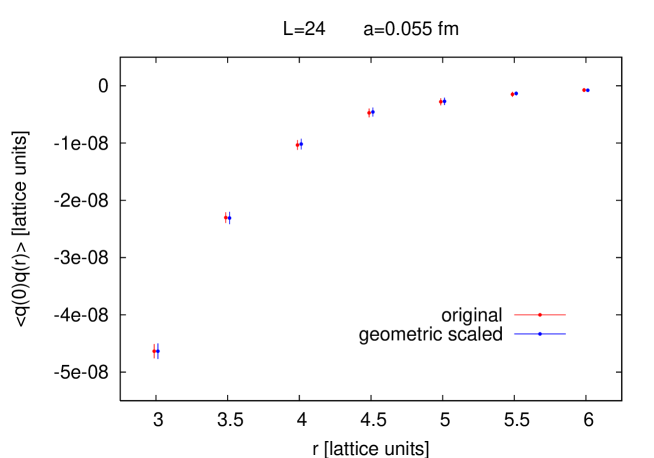
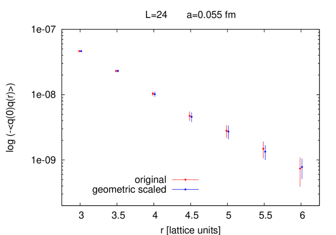
Figure 1: The results for the original, $G(r)$, and the geometric, ${\bar{G}}(r)$, correlators on $24^{4}$ lattice in pure–glue lattice gauge theory (Iwasaki action) at $a=$ 0.055 fm. ${\bar{G}}(r)$ was rescaled to coincide with $G(r)$ at $r=3$.

2. The Basic Observation. Original results put forward in this work are based on the outcome of the following numerical experiment. Consider an ensemble of topological density configurations corresponding to Wilson’s lattice gauge theory at some cutoff. With every configuration ${\cal C}\equiv\{q(x),\;x\in{\twelvebb Z}^{4}\}$ associate a new configuration ${\bar{\cal C}}({\cal C})$ defined via

$${\bar{\cal C}}\,\equiv\,\{\,sq(x)\equiv\mathop{\rm sgn}\bigl{(}q(x)\bigr{)},\;q(x)\in{\cal C}\,\}$$ (1)

where $\mathop{\rm sgn}(y)$ is the sign function. Thus, the configuration ${\bar{\cal C}}$ has field values $\pm 1$ and possesses the same sign–coherent regions as ${\cal C}$. Now, consider the two–point functions of the original $G(x)\equiv\langle q(x)q(0)\rangle$ and of the associated ${\bar{G}}(x)\equiv\langle sq(x)sq(0)\rangle$ ensembles. Is there a definite relation between $G(x)$ and ${\bar{G}}(x)$? Note that we will frequently refer to barred entities as “geometric” (i.e. geometric correlator, geometric ensemble) since the only information kept from the original configuration is the space–time geometry of sign–coherent regions.

In Fig. 1 we show the result of such calculation on $24^{4}$ lattice at lattice spacing $a=$ 0.055 fm, using overlap–based definition of topological density. Since the overall magnitudes of the two correlators will evidently be very different, we have rescaled the geometric one such that at $|x|\equiv r=3$ they become equal, i.e. ${\bar{G}}(r)\longrightarrow{\bar{G}}(r)G(3)/{\bar{G}}(3)$. On the bottom plot, we show the results on a logarithmic scale to better discern points at larger distances. As can be seen quite clearly, the original and the rescaled geometric 2–point functions appear identical within statistical errors. In fact the agreement is better than statistical, indicating that, already at this physical volume, sign–coherent geometry drives correlations at the level of individual configurations.

There are couple of points that we would like to note here. Firstly, the feature uncovered above only holds in the “negative part” of the lattice correlator, i.e. in the region where it can approximate the behavior at finite physical distances, and not in the positive core. Indeed, we will not propose that lattice correlators $G(x)$ and ${\bar{G}}(x)$ are equal up to rescaling. Rather, we will conjecture the possibility that they define the same continuum limit at non–zero physical distances. Secondly, we emphasize that the currently available data [8] is supportive of the scenario with geometric dominance being satisfied at all, rather than just at asymptotically large physical distances.

3. Specifics and Formalization. The numerical work on which we draw our conclusions is based on pure–glue SU(3) lattice ensembles defined by the Iwasaki action and specified in Table 1. The referenced lattice spacings are obtained from string tension ($\sqrt{\sigma}=\,$450 MeV), and the physical volume is kept fixed at $V_{p}=3$ fm⁴. For definition of topological density operator we use overlap Dirac matrix [9] based on Wilson–Dirac kernel with standardly defined parameters $r=1$ and $\rho=26/19$. This setup was used in the original work [1] as well as in all the followups by the Kentucky group. Implementation of matrix–vector operation needed to evaluate topological density $q(x)\;=\;\frac{1}{2\rho}\,\mbox{\rm tr}\,\gamma_{5}\,D(x,x)$ is described in Ref. [10].

The correlators shown in Fig. 1 are coarse–grained over the distance of half a lattice spacing. By this we mean that the samples for correlations with a given point were accumulated within the spherical shells of thickness one half, centered at that point. More precisely, let us define a sequence of points and the associated sets (intervals), namely

$$r_{k}\,=\,\cases{\;0\;&\mbox{\rm for $k=0$}\cr\;\frac{k}{2}+\frac{1}{2}\;&\mbox{\rm for $k=1,2,\ldots$}}\qquad{{\twelvefrak I}}_{k}\,=\,\cases{\;\{\,0\,\}\;&\mbox{\rm for $k=0$}\cr\;[\,r_{k}-\frac{1}{4},r_{k}+\frac{1}{4}\,)\;&\mbox{\rm for $k=1,2,\ldots$}\cr}$$ (2)

The coarse–grained correlation function $G(r_{k},{\cal C})$ on a given configuration ${\cal C}$ is defined as

$$G(r_{k},{\cal C})\,=\,\langle\,q(x)q(y)\,\rangle_{\,{\cal C},\,|x-y|\in{{\twelvefrak I}}_{k}}$$ (3)

Continuum limits of the (ensemble–averaged) standard and coarse–grained correlators are the same, but the latter behaves more smoothly which is why we use it here. All conclusions presented here are independent of this choice. In what follows we will denote the coarse–grained correlator simply as $G(r)$ with the above discrete values of $r$ implicitly understood.

The results shown in Fig. 1 correspond to the ensemble ${\cal E}_{4}$ with the ensembles at coarser lattice spacings behaving similarly. To quantify the trends and to formalize the proposed observation, we need a suitable measure. Equality of functions up to a multiplicative constant is naturally expressed in terms of a normalized overlap (scalar product). For continuum real–valued functions $f_{1}$, $f_{2}$ on the interval $[a,b]$ one has

$$\bar{\twelveeusm O}[f_{1},f_{2},a,b]\equiv\frac{f_{1}\cdot f_{2}}{|f_{1}|\,|f_{2}|}\qquad\quad f_{1}\cdot f_{2}\equiv\int_{a}^{b}dx\,f_{1}(x)f_{2}(x)$$ (4)

but in case of fast-decaying functions (such as the correlators considered here) a measure that is more uniform over the domain and more stringent is provided by the “relative overlap”, namely

$${\twelveeusm O}[f_{1},f_{2},a,b]\equiv\bar{\twelveeusm O}\bigl{[}1,\frac{f_{2}}{f_{1}},a,b\bigr{]}$$ (5)

Note that for functions $f(x_{k})$ defined only on discrete set of arguments $x_{k}$ (lattice correlators) we apply the above formulas as well via replacing these functions with their piecewise constant extensions $f(x)=f(x_{k})$ for $x\in[x_{k},x_{k+1})$.

ensemble	$a$ [fm]	$V$	$V_{p}$ [fm4]	configs
$\;{\cal E}_{1}\;$	$\quad 0.110\quad$	$\quad 12^{4}\quad$	$\quad 3.0\quad$	$\quad 142\quad$
$\;{\cal E}_{2}\;$	$\quad 0.082\quad$	$\quad 16^{4}\quad$	$\quad 3.0\quad$	$\quad 50\quad$
$\;{\cal E}_{3}\;$	$\quad 0.066\quad$	$\quad 20^{4}\quad$	$\quad 3.0\quad$	$\quad 20\quad$
$\;{\cal E}_{4}\;$	$\quad 0.055\quad$	$\quad 24^{4}\quad$	$\quad 3.0\quad$	$\quad 10\quad$

Table 1: Ensembles of Iwasaki gauge configurations for topological density calculations.

Consider the lattice definition of the topological density 2–point function in the domain of physical distances $[r_{p,1},r_{p,2}]$. This requires studying the behavior of $G(r,a)$ on the ever–growing sliding lattice interval $[\,r_{p,1}/a,\,r_{p,2}/a\,]$ close to the continuum limit $a\to 0$. If the original and the geometric correlators ($G(r,a)$, ${\bar{G}}(r,a)$) carry the same information about the shape of the physical 2-point function in the continuum limit, their relative overlap has to approach unity. The result of such calculation for the interval [0.15 fm, 0.30 fm] is shown in Fig. 2. To understand this, we also included two ensembles coarser than ${\cal E}_{1}$, with relevant lattice interval being entirely within the positive core of the correlator. For ${\cal E}_{1}$ the upper limit of the interval involves a correlation very close to zero as the correlator just becomes negative. This results in the observed dip and large fluctuation of the relative overlap whose definition implicitly assumes that $f_{1}$ is non–zero on its domain (see Eq. (5)). For finer lattice spacings the relative overlap quickly approaches unity. Given these results, we propose to consider the possibility that the following conjecture holds.

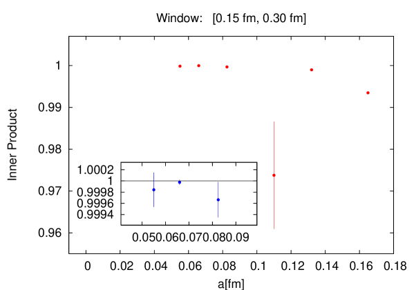
Figure 2: The relative overlap ${\twelveeusm O}[{\bar{G}}(a),G(a),0.15/a,0.30/a]$. See the discussion in the text for explanation.

Conjecture 1. Consider the pure-glue lattice gauge theory defined by the Iwasaki gauge action on the infinite lattice together with arbitrary non–perturbative procedure of fixing the lattice spacing $a$. If $G(a)$ and ${\bar{G}}(a)$ are the original and the geometric 2–point functions of standard overlap–based topological density then

$$\lim_{a\to 0}{\twelveeusm O}\bigl{[}\,{\bar{G}}(a),\,G(a),\,\frac{r_{p,1}}{a},\,\frac{r_{p,2}}{a}\,\bigr{]}\,=\,1$$ (6)

for arbitrary range of physical distances $[r_{p,1},r_{p,2}]$.

We emphasize that we do not mean to imply that the simplest sign reduction $q(x)\rightarrow\mathop{\rm sgn}(q(x))$ considered here is the unique way to obtain the above–proposed equivalence. Rather, what we wish to convey is that there exists a family of computable configuration–based reductions $\{\,q(x)\,\}\rightarrow\{\,sq(x)\,\}$ with $sq(x)\in\{-1,1\}$ such that the shape equivalence holds.

4. The Uses and the Discussion. Dominance of sign–coherent geometry promises to have interesting ramifications regardless of whether it eventually turns out to be an approximation (exact at asymptotically large physical distances) or an exact statement specified by Conjecture 1. In the former case, it suggests to consider the “homogeneous approximation” to fundamental topological structure [8]. In the latter case (strictly consistent with the data at this point) it would represent a simple explicit link between short and long–distance physics – a connection that the fundamental structure (in any composite field) has to encode in some way. There are several possible ways to exploit such exact link, and we mention two examples here. (1) Validity of Conjecture 1 would imply that for spectral calculations (glueball masses) it is sufficient to evaluate configurations of signs of topological density rather than their precise values. For overlap–based topological density, this could lead to a speedup of calculations. (2) An alternative (not strictly equivalent) way of formulating the observed trends is the following. Consider $\lim_{r\to\infty}G(r,a)/{\bar{G}}(r,a)$. This limit, ${\bar{q}}^{2}(a)$, exists and the correlators $G(r,a)$ and ${\hat{G}}(r,a)\equiv{\bar{G}}(r,a){\bar{q}}^{2}(a)$ are strictly equivalent from the point of view of the continuum limit. In particular, in the expected way of obtaining finite physical 2-point function we have at arbitrary physical distance $r_{p}$

$$G_{p}(r_{p})\equiv\lim_{a\to 0}\frac{G(\frac{r_{p}}{a},a)}{a^{8}}\,=\,\lim_{a\to 0}\frac{{\hat{G}}(\frac{r_{p}}{a},a)}{a^{8}}\,=\,\lim_{a\to 0}\frac{{\bar{G}}(\frac{r_{p}}{a},a)\,{\bar{q}}^{2}(a)}{a^{8}}$$ (7)

Applying this equation to short distances $x_{p}\ll 1/m_{p}$ (glueball range) and taking into account that ${\bar{G}}(r,a)$ has finite continuum limit at fixed $r$, one can see that measuring ${\bar{q}}^{2}(a)$ offers a novel way of testing the exact nature of asymptotic freedom. In Fig. 3 we show the result of evaluating ${\bar{q}}^{2}(a)$ for ensembles ${\cal E}_{1}$–${\cal E}_{4}$ (fitting $G(r,a)/{\bar{G}}(r,a)$ to a constant), indicating that for our finest lattices (2.3–3.6 GeV) the behavior is excellently described by ${\bar{q}}^{2}(a)\propto a$. The perturbative prediction, namely a logarithmic decrease of ${\bar{q}}^{2}(a)$ toward zero, hasn’t yet set in. It will be quite interesting to examine yet shorter scales to see where the perturbative description starts to dominate, and to look for possible geometric changes occurring in the fundamental structure as that happens. The absence of such transition would imply a highly non–standard scenario, in which $G_{p}(x_{p})\propto 1/|x_{p}|^{7}$ at short distances with the true dimension of the topological density operator being $D_{q}=3.5$ rather than $D_{q}=4$. In that case the parameter $\theta$ would be dimensionful (analogous to mass), asymptotic freedom would be only approximate, and the strong CP problem would cease to exist.

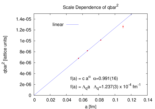
Figure 3: The scale dependence of ${\bar{q}}^{2}(a)$.See the discussion in the text for explanation.

References

- [1] I. Horváth et al., Phys. Rev. D68, 114505 (2003).
- [2] A. Alexandru, I. Horváth, J.B. Zhang, Phys. Rev. D72 (2005) 034506.
- [3] I. Horváth, hep-lat/0605008; hep-lat/0607031; “Framework for Systematic Study of QCD Vacuum Structure III: Scale Dependence”, in preparation.
- [4] P.Y. Boyko, F.V. Gubarev, Phys. Rev. D 73, 114506 (2006).
- [5] E.M. Ilgenfritz, et al., Phys. Rev. D76, 034506 (2007).
- [6] I. Horváth, et al., Phys. Lett. B612 (2005) 21.
- [7] S. Ahmad, J.T. Lenaghan, H.B. Thacker, Phys. Rev. D72, 114511 (2005); H.B. Thacker, PoS LAT2005 (2005) 324, hep-lat/0509057; F.L. Lin, S.Y. Wu, arXiv:0805.2933; P.J. Moran, D.B. Leinweber, arXiv:0805.4246.
- [8] I. Horváth, A. Alexandru, T. Streuer, in preparation.
- [9] H. Neuberger, Phys. Lett. B417 (1998) 141; Phys. Lett. B427 (1998) 353.
- [10] Y. Chen et al., Phys. Rev. D70, 034502 (2004).