Revealing components of the galaxy population through nonparametric techniques

Abstract

The distributions of galaxy properties vary with environment, and are often multimodal, suggesting that the galaxy population may be a combination of multiple components. The behaviour of these components versus environment holds details about the processes of galaxy development. To release this information we apply a novel, nonparametric statistical technique, identifying four components present in the distribution of galaxy H$\alpha$ emission-line equivalent-widths. We interpret these components as passive, star-forming, and two varieties of active galactic nuclei. Independent of this interpretation, the properties of each component are remarkably constant as a function of environment. Only their relative proportions display substantial variation. The galaxy population thus appears to comprise distinct components which are individually independent of environment, with galaxies rapidly transitioning between components as they move into denser environments.

1 Components of the galaxy population

It has long been recognised that galaxies may be divided into at least two distinct sub-populations. Originally this division was based on visual appearance. Most galaxies can be morphologically classified as either elliptical or spiral. Finer classification is possible, discretizing an apparently continuous variation in galaxy appearance. However the dichotomy between elliptical and spiral morphology is more pronounced than the variations within each class. Subsequently, it has been discovered that several other, more quantitative, galaxy properties are distributed unevenly or in a multi-modal manner.

The colour distribution of SDSS galaxies is strongly bimodal (Strateva et al., 2001). Galaxies in the “red” and “blue” modes can be roughly identified as those with elliptical and spiral morphology, respectively (Hogg et al., 2002; Driver et al., 2006). Whereas morphology reflects the dynamical state of galaxies, colour is related to their star-formation history, particularly over the last $\la 10^{9}$ years. The colour bimodality thus implies a division of the galaxy population into blue galaxies, which have recently formed stars, and red galaxies, which have not. Such a bimodality in the star-formation properties of galaxies has also been observed using more direct measures of current star-formation, such as emission-line strength (Balogh et al., 2004).

The position of the red and blue galaxy sequences in the colour–luminosity or colour–stellar mass planes display only a weak dependence on environment. However, the relative proportions of galaxies in the two sequences vary strongly. In regions with a higher local galaxy density the fraction of galaxies on the red sequence is higher (Balogh et al., 2004; Baldry et al., 2004; Baldry et al., 2006).

It remains a matter of debate whether colour is more closely related to environment than morphology. Some claim that trends in morphology versus environment can be mostly explained via a morphology–colour relation which is almost independent of environment (Weinmann et al., 2006; Blanton et al., 2006; Ball et al., 2006; Wolf et al., 2007). However, other studies oppose this view (Park et al., 2007), and it has been clearly shown that the colour and morphology bimodalities behave differently with respect to environment and stellar mass (Bamford et al., 2008).

There are growing indications that, in a fraction of the galaxy population, star-formation must be terminated rapidly (Balogh et al., 2004; Baldry et al., 2006). The emission lines in galaxy spectra provide a way of measuring the level of current star formation on a timescale of $\la 10^{7}$ years. They therefore trace rapid star formation variations more sensitively than colour. Another important property of emission lines is that they are produced by active galactic nuclei (AGN), in addition to star formation. AGN are present in many galaxies, and are thought to be produced by accretion of material onto the super-massive black holes which appear to reside at the centre of most, if not all, galaxies (Richstone et al., 1998). Recently a variety of studies have suggested that AGN strongly influence star-formation in their host galaxies, and thus play an important role in defining the galaxy population (Kauffmann et al., 2003; Silk, 2005; Croton et al., 2006; Bower et al., 2006). The potential presence of an AGN contribution complicates the traditional usage of emission-lines as an indicator of star formation rate (SFR). However, it also presents an opportunity to study these two interdependent processes, star-formation and AGN, through the distribution of a single quantity.

Galaxies with contrasting properties are found to be distributed differently in space. Elliptical galaxies cluster together more strongly than spirals (Beisbart & Kerscher, 2000; Giuricin et al., 2001). Similarly, red galaxies are preferentially found in denser environments than blue galaxies (Zehavi et al., 2005). We have a well developed theory for how structure forms in the cosmos, at least in terms of the underlying cold dark matter which dominates the mass density (Springel et al., 2005). Baryonic matter is expected to be similarly distributed, in broad terms. This theory thus explains the range of galaxy environments observed. However, the properties of galaxies as a function of environment is a much more complicated issue, depending on the detailed physics of galaxy formation and evolution. By studying trends in the galaxy population with environment we can learn about these physical processes.

There has been a logical progression in studies of galaxy properties as a function of environment. Early work was based on dividing galaxies into simple classes and looking at variations in the fractions of galaxies of each class in bins of environment (Dressler et al., 1985). As galaxy samples grew, this moved on to examining trends in the mean properties of galaxies as a smooth function of local galaxy density (Lewis et al., 2002; Gómez et al., 2003). A significant development was fitting to the data functions that describe the distribution of galaxies in two classes (Balogh et al., 2004; Baldry et al., 2004; Baldry et al., 2006). Most of the approaches employed so far have relied upon enforcing a predefined view of how to divide or classify the galaxy population in increasingly complex ways. However, our understanding of the physical processes at work is highly uncertain and does not provide a sufficient basis to make this decision. Our only guide is the data itself. A natural next step is thus to turn to nonparametric methods, where the components of the population are deduced consistently from the data itself.

Recently, several studies have performed multivariate statistical analyses on datasets containing a wide variety of galaxy properties, in order to identify components of the galaxy population, and determine which properties are most important for identifying to which component a galaxy belongs (Ellis et al., 2005; Conselice, 2006). Such studies are highly informative, but become complicated when one wishes to determine the behaviour of the identified components versus another variable. In this paper we are primarily concerned with variation in the components of the galaxy population as a function of environment. The statistical method we present below may be straightforwardly applied to multivariate datasets. However, for simplicity, in the present work we consider the environmental dependence of just one galaxy property. Nevertheless, even with this elementary approach, we are able to learn much about the galaxy population.

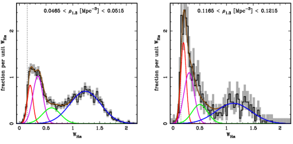
Figure 1: The distribution of transformed H$\alpha$ equivalent width ($W_{\rm{H}\alpha}$) for (left) low and (right) high density environments. The histogram displays the data, with Poisson uncertainties indicated by the grey shading. The red, purple, green and blue lines show the components derived by applying the NMR technique. The brown line gives the sum of these components, which is clearly a good representation of the data.

2 Conditional density estimation

A common problem in astronomy, and statistical sciences in general, is that one wishes to understand how the behaviour of one variable depends upon another. This is relatively straightforward in the case where there is a single relationship between the variables, albeit with some, possibly variable, scatter or width to the distribution. Much statistical and astronomical literature has been devoted to the development of such regression methods (Weisberg, 2005). However, in the case where multiple components may be present in the overall distribution, each with a different functional dependence on the variables, the situation becomes substantially more difficult. One can still attempt to apply single-component statistical tools, for example nonparametric quantile regression (Koenker & Bassett, 1978; Yu & Jones, 1998), on the whole distribution, but the understanding one gains from such an exercise is limited and sometimes misleading. Alternatively one may individually analyse subsamples selected by defining regions in the parameter space, or preferably using additional information(Cherkassky & Ma, 2005). This approach, however, is unsuitable when the multiple components significantly overlap, or when it is unclear how many components are present.

Most regression techniques focus on estimating the conditional mean, the average value of one variable as a function of another variable; for example, a line through a set of scattered points. However, one may get a better understanding of the relationship between a response variable and a set of covariates by considering the estimation of the conditional density as a whole; the distribution of one variable as a function of another. (Note that density here refers to probability density as a function of the parameter set, not a measure of environmental local galaxy density as elsewhere in this paper.) We use a new conditional density estimator based on finite mixture models and local likelihood estimation, which describes the underlying relationship between two variables by a set of parameterised functions. This feature gives the proposed procedure the advantage of being easily interpretable. This method is called nonparametric mixture regression (NMR), and is described in detail in Appendix A.

The NMR technique has the potential to aid the understanding of many datasets, across all fields of science. In the present work, it allows us to determine the environmental dependence for individual components of the galaxy population, with minimal prior assumptions on the number and properties of these components.

3 Galaxy H$\alpha$ equivalent widths

The strongest emission line in a galaxy optical spectrum is H$\alpha$. The luminosity of H$\alpha$ is approximately proportional to the rate of ongoing star-formation (Moustakas et al., 2006), when uncontaminated by additional emission, such as from an AGN. A commonly employed quantity is the equivalent width (EW) of a spectral line, the line flux normalised by the continuum flux at the same wavelength. The EW measurement has the advantages of being approximately independent of uncertainties in the spectral flux calibration and any extinction present in both the observed galaxy and our own. The H$\alpha$ line is in the red region of the spectrum, where the continuum is dominated by the light from old stars. The H$\alpha$ continuum flux is therefore roughly proportional to stellar mass, and hence $\rm{EW}(\rm{H}\alpha)$ is approximately proportional to the SFR per unit stellar mass.

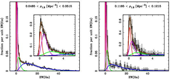
Figure 2: As Fig. 1, but shown here in terms of the untransformed equivalent width, $\rm{EW}(\rm{H}\alpha)$. The inset shows the same plot with axis-ranges chosen to better show the behaviour at small $\rm{EW}(\rm{H}\alpha)$.

The overall distribution of galaxy H$\alpha$ luminosity, equivalent width, and hence absolute and normalised SFR, are found to move to lower levels with increasing environmental density (Lewis et al., 2002; Gómez et al., 2003). This generally agrees with the colour and morphology trends described above, and the variation of H$\alpha$ emission with morphological type (Nakamura et al., 2004). However, if the galaxy population is separated into galaxies which are star-forming and those which are not, the distribution of $\rm{EW}(\rm{H}\alpha)$ for each component does not depend significantly on environment. Only the relative proportion of star-forming galaxies changes strongly (Balogh et al., 2004) with environment. This finding, of distinguishable components in the galaxy population with properties independent of environment but proportions which vary strongly, mirrors the behaviour found in the colour distribution. It also motivates us to perform a more rigorous evaluation of the components present in the galaxy population in this work.

As mentioned earlier, an important feature of emission lines is that, in addition to star formation, they are also produced by AGN. Galaxies whose emission lines are dominated by star-formation or AGN activity can be separated using various diagnostic diagrams. The most common of these plots the emission line ratios ${\rm{[OIII]}\lambda 5007}/{\rm{H}\beta}$ versus ${\rm{[NII]}\lambda 6583}/{\rm{H}\alpha}$, and is known as the BPT diagram (Baldwin et al., 1981). The usual approach is to use these diagrams to reject objects inappropriate to the particular study. Thus a study of galaxy star formation properties would exclude all galaxies with signs of AGN contamination. However, classifying a galaxy using the BPT diagram requires multiple emission lines to be detected, resulting in a fraction of objects which cannot be classified. In addition, the separation between galaxies dominated by star-formation and AGN is not clear, and there appears to be a large population of galaxies which host both star-formation and an AGN. Roughly 20% of all galaxies are unambiguously AGN-dominated, while it is estimated that a further 20% are star-forming galaxies with a significant AGN contribution (Miller et al., 2003). This ambiguity means a variety of SFR–AGN demarcations exist (Kewley et al., 2001; Kauffmann et al., 2003; Stasińska et al., 2006). Star formation studies based on emission lines have therefore rejected widely varying fractions of galaxies from their samples. This fraction is usually low, so significant numbers of AGN-contaminated galaxies remain. More importantly, if our aim is to gain knowledge of star-formation properties across the whole galaxy population, then we may be rejecting an important fraction of the population. If there are any intrinsic correlations between AGN and star-formation, as has been suggested by other studies (Kauffmann et al., 2003), then information about these will be lost.

A number of classes of AGN have been identified. A primary distinction is between Type 1 and Type 2 AGN. In Type 1 objects our viewing angle is such that we see the region immediately around the central black hole directly, and thus the galaxy’s light is dominated by the AGN emission. In this case the properties of the host galaxy are generally very difficult to determine. In Type 2 AGN, the central region is obscured by a dusty torus surrounding it. The observed AGN emission is therefore due to material further removed from the central ionising source, and mostly confined to emission lines. Most photometric and structural galaxy properties may therefore be reliably measured, despite the presence of a Type 2 AGN. In this work we exclude all Type 1 AGN, identified by the large widths of their emission lines, and consider only the more common Type 2 objects. A further subdivision within Type 2 AGN is between LINER and Seyfert 2 objects. These are similar, and may simply be two parts of a continuum of objects, with Seyfert 2 AGN being more powerful and highly ionised. However, there are signs that LINERs and Seyfert 2 AGN are truly physically distinct classes (Kewley et al., 2006).

In this work we examine the components in the distribution of galaxy $\rm{EW}(\rm{H}\alpha)$, interpretable as a proxy for star formation rate and nuclear activity per unit stellar mass. It is possible to estimate the true star-formation rate and stellar mass, for galaxies which do not host an AGN, using a combination of several spectral features. However, such estimates are sensitive to the details of the assumed model. There is therefore a concern that any finding concerning the components of the resulting distribution may be attributable to the model. The $\rm{EW}(\rm{H}\alpha)$, on the other hand, is a single, robust, model-independent measurement.

The data we use in our study is from Data Release 4 of the SDSS (Adelman-McCarthy et al., 2006). The emission line fluxes, continua and resulting EW used in this study are those provided for DR4 by the MPA-Garching group (Tremonti et al., 2004). All quantities used in this paper were obtained from the CMU-PITT SDSS DR4 Value Added Catalog (VAC). The SQL code for the selection of each of our samples is given in Table 1. We construct a volume-limited sample by selecting galaxies with $0.05<z<0.095$ and $M_{r}<-20.4$. In this work we thus focus on the behaviour of fairly bright galaxies. The lower redshift limit ensures the spectra are based on a reasonable fraction of the galaxies’ light; at $z=0.05$ the $3$ arcsec diameter of each spectroscopic fibre corresponds to $3$ kpc. Throughout we convert to physical scales assuming a flat Friedman-Robertson-Walker cosmology with $\Omega_{m}=0.3$, $\Omega_{\lambda}=0.7$ and $H_{0}=70$ km s^-1 Mpc^-1.

Table 1: Definitions of the galaxy samples used in this study, given as ‘where’ clauses of the SQL queries of the CMU-PITT SDSS DR4 VAC

sample	SQL selection	$n$
density defining sample	!z between 0.02 and 0.10 and absolute_Petro_r <= -20.4 and Sort = 0	117873
$\rho_{1.3}$ sample	!z between 0.05 and 0.095 and absolute_Petro_r <= -20.4 and 2.4 < Dist_right_edge and 2.4 < Dist_left_edge and 2.4 < Dist_upper_edge and 2.4 < Dist_lower_edge and H_ALPHA_FLUX > -99 and H_ALPHA_CONT > 0.0001 and H_ALPHA_FLUX/H_ALPHA_CONT > -0.4 and absolute_Petro_u > -990 and absolute_Petro_r > -990 and Sort = 0	76420
$\rho_{5.5}$ sample	!z between 0.05 and 0.095 and absolute_Petro_r <= -20.4 and 11 < Dist_right_edge and 11 < Dist_left_edge and 11 < Dist_upper_edge and 11 < Dist_lower_edge and H_ALPHA_FLUX > -99 and H_ALPHA_CONT > 0.0001 and H_ALPHA_FLUX/H_ALPHA_CONT > -0.4 and absolute_Petro_u > -990 and absolute_Petro_r > -990 and Sort = 0	46998

4 Measuring galaxy environment

Galaxy environment can be characterised in many ways, but a commonly adopted value is the local number density of galaxies brighter than a given luminosity, averaged over some volume or kernel. We estimate the local galaxy number density, $\rho_{b}$, within a fixed-scale, spherical kernel with a Gaussian radial profile and bandwidth $b$. Our local galaxy densities are thus simple to interpret physically.

To select the bandwidth, or scale, $b$ of the kernel, we apply leave-one-out cross-validation; that is, we select the value of $b$ which minimizes the estimated integrated mean squared error, $CV(b)$. This error is obtained by estimating the density function $n$ times, each time leaving out one galaxy from the estimation:

$$CV(b)=\int\widehat{f}_{n,b}^{\;2}(\mn@boldsymbol{x})d\mn@boldsymbol{x}-\frac{2}{n}\sum_{i=1}^{n}\widehat{f}_{(-i),b}(\mn@boldsymbol{X_{i}})$$ (1)

where $\{\mn@boldsymbol{X_{i}}\}$ is the set of galaxy positions, and $\widehat{f}_{n,b}$ and $\widehat{f}_{(-i),b}$ are the kernel density estimators with bandwidth $b$, using all $n$ galaxies and after removing the $i^{\mathrm{th}}$ galaxy, respectively. We compute $CV(b)$ for a range of different bandwidth values to find that which minimizes the error. Applying this cross-validation method we determine an optimum bandwidth value of $1.3$ Mpc. A similar optimum bandwidth for local galaxy density estimation was found using cross-validation by Balogh et al. (2004).

Interestingly, this scale corresponds to the size of galaxy clusters, and is thus highly appropriate for characterising density from a physical, as well as a statistical, point of view. However, while cross-validation provides the statistically optimum bandwidth for the whole sample, any choice of bandwidth has its limitations. This density estimator loses resolution at low densities, where there are no neighbouring galaxies within the kernel bandwidth, and is thus unable to discriminate between densities lower than $\rho_{1.3}\sim 0.03$ Mpc^-3, comprising 17% of the sample. In order to probe environments less dense than this, but necessarily on larger physical scales, we additionally perform the analysis with local densities measured using a larger bandwidth of $5.5$ Mpc. Almost all galaxies have a neighbour within this radius. One could also consider estimating densities with a kernel bandwidth significantly smaller than $1.3$ Mpc. However, such an estimator would lose resolution below even moderate densities, where galaxies are typically separated by more than the bandwidth. It would also be less able to discriminate between high density environments, because the densities are estimated using galaxy positions uncorrected for redshift-space distortions, and hence an increase in true-space density no longer results in a higher redshift-space density within the kernel. We mostly show results based on the statistically-motivated $1.3$ Mpc bandwidth in the main body of this article, but provide figures using the $5.5$ Mpc bandwidth in Appendix B, to demonstrate that we find similar results on larger scales and to lower densities.

We avoid biased density estimates for galaxies at the edges of our sample volume by determining the densities using a larger volume sample of galaxies with $0.02<z<0.10$ and $M_{r}<-20.4$. We then limit the analysis sample to galaxies with $0.05<z<0.095$ and further than approximately twice the bandwidth from a survey boundary. We reject a further 3% of galaxies with unreliable $\rm{EW}(\rm{H}\alpha)$ or $(u-r)$ rest-frame colour measurements. The exact selections, and corresponding sample sizes, are given in Table 1.

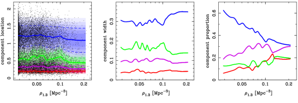
Figure 3: The behaviour of the NMR components versus environment. The left panel plots the data as dots, along with the location of each component, indicated by thick, solid lines, and additionally their widths via the coloured shading and dashed lines. These widths are shown explicitly in the middle panel. The right panel displays the variation in the proportion of each component. While the location and width of the components do not change significantly with environment, the proportions vary strongly.

5 Applying the NMR technique

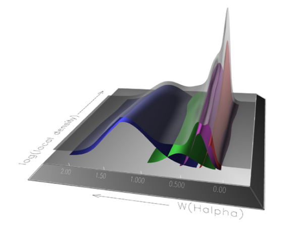
Figure 4: A three-dimensional view of the NMR estimate of the $W_{\rm{H}\alpha}$–$\rho_{5.5}$ distribution, shown by the grey, transparent surface, and its constituent components, colour-coded is in the previous figures. It can be clearly seen that the positions and widths of the components do not change significantly, while their relative proportions vary substantially.

A brief inspection of the sample $\rm{EW}(\rm{H}\alpha)$ distribution reveals a peak around zero EW, with a long, asymmetric tail to high EW. The NMR technique is more computationally efficient when using symmetrical, Gaussian functions to model the distribution. Gaussians are also an obvious choice due to their exceptional richness and flexibility. For convenience we therefore wish to transform the equivalent width quantity to a space where its natural components appear to take a more symmetrical, Gaussian, form. Better matching the shape of the true distribution components to that assumed in the NMR technique will also naturally result in fewer NMR components being required to model the distribution (but see Appendix A). The EW extend slightly to negative values, proscribing a simple logarithmic transformation. We therefore choose the transformation $W_{\rm{H}\alpha}=\log_{10}(\rm{EW}(\rm{H}\alpha)+\lambda)$. The zero offset parameter, $\lambda$, must be large enough to make the logarithm argument positive for the most negative EW value in our sample. In constructing our sample we remove outliers by requiring $\rm{EW}(\rm{H}\alpha)>-0.4$, thereby clipping the lowest 0.1% of the sample. Therefore, we must have $\lambda>0.4$. We have examined the behaviour of our NMR fits and their likelihood with variations in $\lambda$. The chosen value has only a relatively small effect, slightly altering the shape of the Gaussian basis functions once they are transformed back into EW space, but not changing our results significantly. Here we adopt $\lambda=1.4$ as a compromise between maximising the fit likelihood and ensuring stable behaviour. We must also choose a reasonable bandwidth for the regression kernel in $\rho$. Following extensive tests we adopt an adaptive bandwidth enclosing the nearest 5000 points (also see discussion in Appendix A).

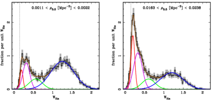
Figure 8: As Fig. 1, but for local galaxy densities estimated using a $5.5$ Mpc bandwidth kernel, $\rho_{5.5}$. The results are very similar to those found using $\rho_{1.3}$.

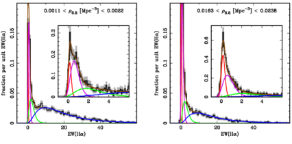
Figure 9: As Fig. 8, but shown in terms of the untransformed equivalent width, $\rm{EW}(\rm{H}\alpha)$. The inset shows the same plot with axis-ranges chosen to better show the behaviour at small $\rm{EW}(\rm{H}\alpha)$.

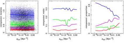
Figure 10: As Fig. 3, but for local galaxy densities estimated using a $5.5$ Mpc bandwidth kernel, $\rho_{5.5}$. The results are very similar to those found using $\rho_{1.3}$.

We apply the NMR technique to the distribution of $W_{\rm{H}\alpha}$, and determine the optimum number of components using the Bayesian Information Criterion (BIC; Schwarz, 1978). Four components are strongly preferred by the data, by $\Delta$BIC $>$ 7 (see Appendix A for more details). In Fig. 1 (Fig. 8) we show the NMR components we obtain for the $\rho_{1.3}$ ($\rho_{5.5}$) sample, at two values of local galaxy density. The components are plotted in $W_{\rm{H}\alpha}$-space, in which the technique is applied. We also show the components and data transformed back into $\rm{EW}(\rm{H}\alpha)$-space in Fig. 2 (Fig. 9). The properties of these components as a function of environmental density are shown in Fig. 3 (Fig. 10). In Fig. 4 we show a three-dimensional view of the components and their sum for the $\rho_{5.5}$ sample, which includes all the relevant information (location, width and relative proportion of each component) in a single plot. We show the results for the $\rho_{5.5}$ here simply because they are smoother than those for $\rho_{1.3}$, and the individual components are more clearly visible in this three-dimensional view. It is critical to note that the only data which has been used to determine these components is the $\rm{EW}(\rm{H}\alpha)$ distribution.

At this stage we make no attempt at interpreting the components as physically distinct populations. Nevertheless, Figs. 1, 8, 2, 9 indicate that the $\rm{EW}(\rm{H}\alpha)$ distribution can be well described by multiple components. The hypothesis that the galaxy population comprises distinct components, or types, is strongly supported by the various property bimodalities described earlier. We find that the locations and widths of the components of the $\rm{EW}(\rm{H}\alpha)$ distribution are independent of environment. Only the relative proportions of the components are found to vary strongly. This implies that the variations with environment are primarily the result of differences in the relative frequency of each galaxy type, rather than changes in the intrinsic properties of each type.

Galaxies move to regions of higher density over time, under the influence of gravity. The variation of galaxy properties with environment is therefore at least partly due to environmentally-dependent changes in individual galaxy properties over time. If all galaxies in a given environment were affected similarly, we would expect to see smooth changes in the property distributions of each individual component. However, we find that the individual components remain mostly unchanged with environment. This implies that some galaxies are transformed directly from one type to another, in an apparently stochastic manner. If this transformation is sufficiently slow, we would expect to see the transitioning galaxies appearing as a separate component in the relevant range of local density. If it is rapid, then the fraction of transitioning galaxies at any time would be too low to separate from the main distribution.

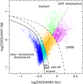
Figure 5: The BPT diagram for our $\rho_{1.3}$ sample, traditionally used to identify star-forming galaxies and AGN hosts. For clarity, only one-fifth of our sample galaxies are plotted. The LINER, Seyfert 2 and SF dominated regions are colour-coded to match our interpretation of their correspondence to the NMR components shown in the other figures (purple, blue and green, respectively). Note that many galaxies cannot be placed on this diagram. These are passive galaxies, with no emission lines, and uncertain galaxies, with some detected emission lines, but not all four of those required for inclusion in this diagram.

6 Identifying the components

It is easy to identify the component at zero $\rm{EW}(\rm{H}\alpha)$ with passive galaxies, containing no star-formation or AGN activity. The dominant component at high $\rm{EW}(\rm{H}\alpha)$ must be associated with star-forming galaxies (with the above caveats concerning potential AGN contamination). We also find two intermediate $\rm{EW}(\rm{H}\alpha)$ components. The principle change with environment appears to be the movement of galaxies from the star-forming component to the others, but primarily to the passive component. However, interpreting either of these intermediate EW components as a population transitioning between star-forming and passive is inconsistent with their existence as a significant fraction of the galaxy population even at low environmental densities.

To explore the physical interpretation of the components we have found, we now turn to more traditional diagnostics to separate the contributions from star formation (SF) and AGN to the emission lines. The BPT diagram for our $\rho_{1.3}$ sample is shown in Fig. 5. In order to appear on this plot, all four required emission lines must be detected at $>2$ sigma significance. The classifications we define are as follows; passive: no emission lines detected, SF dominated: all four lines detected and below the curve of Stasińska et al. (2006), AGN dominated: above the line of Kewley et al. (2001) with either all four lines detected or with both lines for just one of the ratios detected and ${\rm{[OIII]}}/{\rm{H}\beta}>0.6$ or ${\rm{[NII]}}/{\rm{H}\alpha}>0.05$, AGN+SF: all four lines detected and between the curves of Kewley et al. (2001) and Kauffmann et al. (2003), SF+AGN: all four lines detected and between the curves of Stasińska et al. (2006) and Kauffmann et al. (2003), uncertain: at least one of the four emission lines detected, but none of the other classification criteria met. Note that the majority of AGN-dominated galaxies can be robustly identified simply from their ${\rm{[NII]}}/{\rm{H}\alpha}$ ratio (Miller et al., 2003; Stasińska et al., 2006).

Our classification method is such that galaxies classified as AGN dominated must contain a significant AGN component, and will have low contribution to their emission lines from star formation. On the other hand SF dominated galaxies may well also contain up to $\sim 20$–$40$% AGN contamination in their emission lines (Kauffmann et al., 2003; Stasińska et al., 2006). The AGN dominated galaxies can be further subdivided into LINER and Seyfert 2 sources using the BPT diagram (Kauffmann et al., 2003).

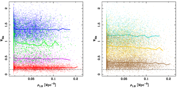
Figure 6: The $W_{\rm{H}\alpha}$–$\rho_{1.3}$ distribution for objects in our sample colour-coded by their location in the BPT diagram shown in Fig. 4. The lines indicate the median $W_{\rm{H}\alpha}$ in bins of $\rho_{1.3}$ for each subsample. The left panel shows passive, LINER, Seyfert 2 and SF dominated galaxies (in order of increasing $W_{\rm{H}\alpha}$), while the right panel shows uncertain, AGN+SF and SF+AGN galaxies (brown, orange and cyan, respectively, and again in order of increasing $W_{\rm{H}\alpha}$). A comparison with Fig. 2 reveals a correspondence between the NMR components and, in order of increasing $W_{\rm{H}\alpha}$, (1) passive galaxies, (2) LINER and uncertain galaxies, (3) Seyfert 2 and AGN+SF galaxies, and (4) SF dominated and SF+AGN galaxies.

Figure 6 shows the $W_{\rm{H}\alpha}$–$\rho_{1.3}$ distributions of galaxies classified using the BPT diagram. Comparing with Fig. 3, one can clearly identify the NMR components with the passive, LINER, Seyfert 2 and SF dominated BPT-classified galaxies. The large fraction of galaxies for which the BPT diagram gives an uncertain result may also be identified with the components. The galaxies with apparently mixed star formation and AGN emission are found at similar $W_{\rm{H}\alpha}$ to the Seyfert 2 objects, and the higher intermediate NMR component. Galaxies with at least one emission line, but which cannot be identified via the BPT diagram have similar $W_{\rm{H}\alpha}$ to LINER objects and the lower NMR component. While not conclusive, this strongly suggests that the components derived from the NMR technique do represent physically distinct populations. This is remarkable given that the NMR components have been inferred from just a single emission line.

7 A new insight into the galaxy population

By applying the newly developed NMR method to the H$\alpha$ equivalent width distribution, a single astrophysical quantity that contains information on both star formation and nuclear activity, we have identified four distinct components in the galaxy population. None of these components vary significantly with environment, in terms of the distribution of their H$\alpha$ equivalent widths. However, the relative proportions of galaxies in each component vary substantially with environment. This implies that any environmental processes at work do not affect all galaxies in a gradual way, which would result in changes in the component H$\alpha$ equivalent width distributions. Rather, they must rapidly transform a fraction of galaxies from one component to another, in a stochastic manner, in order to avoid changing the properties of the individual components.

The above conclusions stand without requiring us to identify the components with more traditional galaxy sub-populations. However, when we attempt such an identification, we find that the extreme components may be associated with passive and star-forming galaxies, while the two intermediate components display similarities to galaxies hosting LINERs and Seyfert 2 AGN. Galaxies with an apparent mix of star-formation and AGN may also be identified with these components. However, in contrast to the usual methods of classifying the star-formation and AGN properties of galaxies, which require multiple emission lines to be significantly detected, the technique we describe in this paper is applicable to all galaxies. We thereby avoid the issue of excluding objects for which traditional methods are uncertain, and the biases which this may introduce.

Appendix A Nonparametric mixture regression

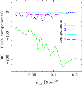
Figure 7: Offsets in the Bayesian Information Criterion (BIC) score versus local galaxy density, $\rho_{1.3}$, for NMR fits utilising 2, 3, and 5 components, relative to the favoured 4 component fit. Where the 5 component fit BIC offset is zero at low $\rho_{1.3}$, the NMR method only uses 4 of the 5 available components as two of the components are degenerate. Four components are thus preferred, by significantly higher BIC values, at all local densities.

This is a newly developed statistical method for determining the dependences of one variable, $y$, on another, $x$, where there may be multiple components present in the data, each with a different $y$ on $x$ dependence. For the analysis presented in the main body of this article we use this technique, putting $x=\rho_{1.3}$ or $\rho_{5.5}$, estimates of the local environmental density, and $y=W_{\rm{H}\alpha}$, a transformed version of the H$\alpha$ equivalent width (see Section 3). Here we give a technical description of the method.

We model the probability, $f(y|x)$, of $y$ given $x$ as a sum of components, thus

$$f(y|x;{\mn@boldsymbol{\Theta}}(x))=\sum_{i=1}^{c(x)}{\pi_{i}(x)s_{i}(y|{\mn@boldsymbol{\eta}}_{i}(x))}$$ (2)

where the $s_{j}(y|\mn@boldsymbol{\eta}_{j}(x))$, are density functions with a vector of parameters ${\mn@boldsymbol{\eta}}_{j}(x)$ that depends on $x$, and the $\pi_{j}(x)$’s are a set of mixing proportions that sums to one for each $x$. In this paper we use Gaussian functions to model the components, each with parameters ${\mn@boldsymbol{\eta}}_{i}=(\mu_{i},\sigma_{i}$), mean and standard deviation respectively. The number of components is $c(x)$, and may vary as a function of $x$. Gaussians are rich and flexible functions which are highly suited to this task, particularly if one wishes to avoid the danger of overly designing the method to fit one’s expectations of the results.

The parameter set, ${\mn@boldsymbol{\Theta}}(x)\left({\mn@boldsymbol{\theta}}_{1}(x),\ldots,{\mn@boldsymbol{\theta}}_{c(x)}(x)\right)=(\pi_{1}(x),{\mn@boldsymbol{\eta}}_{1}(x),\ldots,\pi_{c(x)}(x),{\mn@boldsymbol{\eta}}_{c(x)}(x))$, is determined using local likelihood estimation. The parameters are approximated locally by a polynomial of degree $p$, and hence vary smoothly with $x$. The variation of the parameters can thus be described by a set of polynomial coefficients, $\mn@boldsymbol{B}$. These coefficients may then be constrained by data, weighted using a kernel of bandwidth $b(x)$ about $x$.

The log-likelihood function of the set of polynomial coefficients $\mn@boldsymbol{B}$ given the data is therefore

$${\cal L}_{p}(\mn@boldsymbol{B};x,b,c(x)) = \sum_{m=1}^{n}w_{m}(x;b)\times$$

$$\log_{e}f(Y_{m},x;\mn@boldsymbol{T}(X_{m}-x,\mn@boldsymbol{B})),$$

for $n$ measurements labelled by $m$, with locations $(x,y)=(X_{m},Y_{m})$. The set of polynomial functions approximating the parameters $\mn@boldsymbol{\Theta}$ at $x$ are

$$\mn@boldsymbol{T}(\delta_{m},\mn@boldsymbol{B})=\big{(}t_{1,1}\big{(}\delta_{m},\mn@boldsymbol{\beta}_{1,1}\big{)},\ldots,t_{1,1}\big{(}\delta_{m},\mn@boldsymbol{\beta}_{1,q_{1}}\big{)},\ldots,$$ (4)

$$t_{c(x),1}\big{(}\delta_{m},\mn@boldsymbol{\beta}_{c(x),1}\big{)},\ldots,t_{c(x),1}\big{(}\delta_{m},\mn@boldsymbol{\beta}_{c(x),q_{c(x)}}\big{)}\big{)},$$

defining $\delta_{m}=X_{m}-x$, with

$$t_{i,j}(\delta_{m},\mn@boldsymbol{\beta}_{i,j})=\sum_{k=0}^{p}{\beta_{i,j,k}(\delta_{m})^{k}/k!},$$ (5)

where $i=1,\ldots,c(x)$ counts over the components, $j=1,\ldots,q_{i}$ counts the parameters of component $i$ (in our case each density function is a Gaussian with parameters $\mu$ and $\sigma$, and with mixing weight $\pi$, thus $q_{i}=3$), and $k=0,\ldots,p$ counts the degrees of the polynomials used in $\mn@boldsymbol{T}$ to approximate the parameters $\mn@boldsymbol{\Theta}$. The $\beta_{i,j,k}$, and hence their containing sets, $\mn@boldsymbol{\beta}_{i,j}$ and $\mn@boldsymbol{B}$, correspond to a particular value of $x$. Note that the $\beta_{i,j,k}$ give approximations around $\delta_{m}=0$ for the value and $k$-th derivative of the parameter $j$ of component $i$. The contribution to ${\cal L}_{p}$ of data at distance $\delta_{m}$ from $x$ is specified by

$$w_{m}(x;b(x))=W\left(\frac{X_{m}-x}{b(x)}\right),$$ (6)

where $W(z)$ is a weighting function.

One can then attempt to determine the $\mn@boldsymbol{B}$ which maximises the local log-likelihood, ${\cal L}_{p}$, which we denote $\widehat{\mn@boldsymbol{B}}(x;b(x),c(x))$, explicitly indicating its dependencies. Therefore,

$$\widehat{\mn@boldsymbol{B}}(x;b(x),c(x))=\begin{array}[]{c}\\ \mathrm{argmax}\\ ^{\mn@boldsymbol{B}}\end{array}\sum_{j=1}^{n}w_{j}(x;b(x))\;\times$$

$$\log_{e}\sum_{i=1}^{c(x)}s_{i}\big{(}Y_{j}|t_{i,1}(X_{j}-x,{\mn@boldsymbol{\beta}}_{i,1}),\ldots,t_{i,q_{i}}(X_{j}-x,{\mn@boldsymbol{\beta}}_{i,q_{i}})\big{)}.$$

The local likelihood estimate for the set of parameters is then defined by $\widehat{\mn@boldsymbol{\Theta}}(x;b(x),c(x))=\mn@boldsymbol{T}(0,\widehat{\mn@boldsymbol{B}}(x;b(x),c(x)))$, that is $\widehat{\theta}_{i,j}(x;b(x),c(x))=\widehat{\beta}_{i,j,0}(x;b(x),c(x))$. Our conditional density estimate given $b(x)$ and $k(x)$ is therefore

$${\widehat{f}}(y|x;b(x),c(x))\equiv f(y|x;{\widehat{\mn@boldsymbol{\Theta}}}(x;b(x),c(x))).$$ (11)

In general, given $b(x)$ and $c(x)$, the standard method of solving Eqn. A is to use the Expectation-Maximisation (EM) method (McLachlan & Krishnan, 1997).

The estimator Eqn. 11 is dependent upon the chosen bandwidth $b(x)$ and number of components $c(x)$. If they are a priori unknown, we must therefore select them in some reliable way.

In this work we have chosen the bandwidth for $x=\rho_{1.3}$ or $\rho_{5.5}$ to be a function of the $K$th nearest neighbour. We use $K=5000$, selected as a compromise between the smoothness of the resulting component regression lines and their ability to trace any variation in $W_{\rm{H}\alpha}$ versus environment. We have checked that the exact choice of $K$ (within the range 1000–7500) does not affect our results. The optimum number of components was determined using the Bayesian Information Criterion(BIC; Schwarz, 1978):

$$\mathrm{BIC}={\cal L}_{p}-\frac{1}{2}(3c-1)\log_{e}(K)$$ (12)

where ${\cal L}_{p}$ is the maximised log-likelihood, $c$ is the number of components, and $K$ is the sample size. With this definition, otherwise known as the Schwarz Criterion, the preferred model is that which maximises the value of BIC. Note that other definitions sometimes multiply the right hand side of Eqn. 12 by $-2$. The difference between the BIC values of two models, $\Delta$BIC, approximates the natural logarithm of the Bayes factor, a summary of the evidence for one model over another. A $\Delta$BIC of 7 indicates that the preferred model is truly better than the alternative model with odds better than a thousand to one. A Bayes factor of $>150$, i.e. $\Delta\mathrm{BIC}>5$, is generally taken to be very strong evidence for the preferred model (Kass & Raftery, 1995). Four components are thus very strongly favoured, by $\Delta$BIC = 147.1, 11.9 and 7.7 versus 2, 3 and 5 components, respectively, averaged over $\log_{10}\rho_{1.3}$. The $\Delta$BIC are shown versus $\rho_{1.3}$ in Fig. 7.

One might argue that choosing different density functions, other than Gaussians, or applying a different transformation, would result in our finding a different optimal number of components. However, when varying the $W_{\rm{H}\alpha}=\log_{10}(\rm{EW}(\rm{H}\alpha)+\lambda)$ transformation by changing $\lambda$, and trying various combinations of Gaussians and lognormal functions in $\rm{EW}(\rm{H}\alpha)$-space, the optimum number of components has consistently turned out to be four. A careful visual inspection of the $\rm{EW}(\rm{H}\alpha)$ and $W_{\rm{H}\alpha}$ distributions also supports this conclusion.

Obviously one could examine the data and devise component density functions that would result in the NMR method finding any desired number of components. However, this defeats the object of employing the NMR technique. By ‘components’ we mean simple, distinct elements of the overall population. We must therefore make only simple assumptions and transformations in order to identify them, with minimal prior reference to the data.

If two or more NMR components together represent only a single true component of the galaxy populations, then we would expect them to behave identically. Otherwise, they could not represent a single component, by definition. However, our four NMR components each demonstrate different behaviour with respect to local density, indicating they are truly distinct (see Figs. 1–3, B1–B3).

Finally, the components we find using the NMR technique correspond remarkably well to traditional galaxy classifications (compare Figs. 3 & 6). This strongly supports our interpretation of the NMR components as physically distinct elements of the galaxy population. However, the NMR components have the advantage of being based on all galaxies in our sample. Traditional diagnostic diagrams can only be used for objects with multiple, significantly-detected, emission lines, and in many cases give ambiguous classifications (e.g. SF+AGN).

Appendix B Larger scale environment

The main text of the paper focuses on a measure of environment using a kernel of bandwidth $1.3$ Mpc, chosen by cross-validation. This bandwidth performs well at the scales of galaxy clusters. However, at low densities there is frequently only one galaxy within the kernel, and the estimator is unable to differentiate between different low-density environments. We thus additionally perform our analysis using local densities estimated using a kernel with $5.5$ Mpc bandwidth. The results are very similar to those from the $1.3$ Mpc densities, and thus our conclusions are robust to the precise definition of local density. The figures corresponding to the $5.5$ Mpc kernel are given in this appendix.

References

- Adelman-McCarthy et al. (2006) Adelman-McCarthy J. K., et al., 2006, ApJS, 162, 38
- Baldry et al. (2004) Baldry I. K., Balogh M. L., Bower R., Glazebrook K., Nichol R. C., 2004, in Allen R. E., Nanopoulos D. V., Pope C. N., eds, The New Cosmology: Conference on Strings and Cosmology Vol. 743 of American Institute of Physics Conference Series, Color bimodality: Implications for galaxy evolution. pp 106–119
- Baldry et al. (2006) Baldry I. K., Balogh M. L., Bower R. G., Glazebrook K., Nichol R. C., Bamford S. P., Budavari T., 2006, MNRAS, 373, 469
- Baldwin et al. (1981) Baldwin J. A., Phillips M. M., Terlevich R., 1981, PASP, 93, 5
- Ball et al. (2006) Ball N. M., Loveday J., Brunner R. J., 2008, MNRAS, 383, 907
- Balogh et al. (2004) Balogh M., et al., 2004, MNRAS, 348, 1355
- Balogh et al. (2004) Balogh M. L., Baldry I. K., Nichol R., Miller C., Bower R., Glazebrook K., 2004, ApJL, 615, 101
- Bamford et al. (2008) Bamford S. P., Nichol R. C., Baldry I. K., Land K., Lintott C. J., Schawinski K., Slosar A., Szalay A. S., Thomas D., Torki M., Andreescu D., Edmondson E. M., Miller C. J., Murray P., Raddick M. J., Vandenberg J., 2008, ArXiv:0805.2612
- Barnes et al. (2006) Barnes D. G., Fluke C. J., Bourke P. D., Parry O. T., 2006, Publications of the Astronomical Society of Australia, 23, 82
- Beisbart & Kerscher (2000) Beisbart C., Kerscher M., 2000, ApJ, 545, 6
- Blanton et al. (2006) Blanton M. R., Berlind A. A., Hogg D. W., 2007, ApJ, 664, 791
- Bower et al. (2006) Bower R. G., Benson A. J., Malbon R., Helly J. C., Frenk C. S., Baugh C. M., Cole S., Lacey C. G., 2006, MNRAS, 370, 645
- Cherkassky & Ma (2005) Cherkassky V., Ma Y., 2005, IEEE Transactions on Neural Networks, 16, 785
- Conselice (2006) Conselice C. J., 2006, MNRAS, 373, 1389
- Croton et al. (2006) Croton D. J., Springel V., White S. D. M., De Lucia G., Frenk C. S., Gao L., Jenkins A., Kauffmann G., Navarro J. F., Yoshida N., 2006, MNRAS, 365, 11
- Dressler et al. (1985) Dressler A., Thompson I. B., Shectman S. A., 1985, ApJ, 288, 481
- Driver et al. (2006) Driver S. P., et al., 2006, MNRAS, 368, 414
- Ellis et al. (2005) Ellis S. C., Driver S. P., Allen P. D., Liske J., Bland-Hawthorn J., De Propris R., 2005, MNRAS, 363, 1257
- Giuricin et al. (2001) Giuricin G., Samurović S., Girardi M., Mezzetti M., Marinoni C., 2001, ApJ, 554, 857
- Gómez et al. (2003) Gómez P. L., et al., 2003, ApJ, 584, 210
- Hogg et al. (2002) Hogg D. W., et al., 2002, AJ, 124, 646
- Kass & Raftery (1995) Kass R. E., Raftery A. E., 1995, Journal of the American Statistical Association, 90, 773
- Kauffmann et al. (2003) Kauffmann G., Heckman T. M., Tremonti C., Brinchmann J., Charlot S., White S. D. M., Ridgway S. E., Brinkmann J., Fukugita M., Hall P. B., Ivezić Ž., Richards G. T., Schneider D. P., 2003, MNRAS, 346, 1055
- Kewley et al. (2001) Kewley L. J., Dopita M. A., Sutherland R. S., Heisler C. A., Trevena J., 2001, ApJ, 556, 121
- Kewley et al. (2006) Kewley L. J., Groves B., Kauffmann G., Heckman T., 2006, MNRAS, 372, 961
- Koenker & Bassett (1978) Koenker R., Bassett G., 1978, Econometrica, 46, 33
- Lewis et al. (2002) Lewis I., et al., 2002, MNRAS, 334, 673
- McLachlan & Krishnan (1997) McLachlan G., Krishnan T., 1997, The EM algorithm and extensions (Wiley series in probability and statistics). John Wiley & Sons
- Miller et al. (2003) Miller C. J., Nichol R. C., Gómez P. L., Hopkins A. M., Bernardi M., 2003, ApJ, 597, 142
- Moustakas et al. (2006) Moustakas J., Kennicutt Jr. R. C., Tremonti C. A., 2006, ApJ, 642, 775
- Nakamura et al. (2004) Nakamura O., Fukugita M., Brinkmann J., Schneider D. P., 2004, AJ, 127, 2511
- Park et al. (2007) Park C., Choi Y.-Y., Vogeley M. S., Gott J. R. I., Blanton M. R., 2007, ApJ, 658, 898
- Richstone et al. (1998) Richstone D., Ajhar E. A., Bender R., Bower G., Dressler A., Faber S. M., Filippenko A. V., Gebhardt K., Green R., Ho L. C., Kormendy J., Lauer T. R., Magorrian J., Tremaine S., 1998, Nature, 395, A14
- Schwarz (1978) Schwarz G., 1978, The Annals of Statistics, 6, 461
- Silk (2005) Silk J., 2005, MNRAS, 364, 1337
- Springel et al. (2005) Springel V., White S. D. M., Jenkins A., Frenk C. S., Yoshida N., Gao L., Navarro J., Thacker R., Croton D., Helly J., Peacock J. A., Cole S., Thomas P., Couchman H., Evrard A., Colberg J., Pearce F., 2005, Nature, 435, 629
- Stasińska et al. (2006) Stasińska G., Cid Fernandes R., Mateus A., Sodré L., Asari N. V., 2006, MNRAS, 371, 972
- Strateva et al. (2001) Strateva I., et al., 2001, AJ, 122, 1861
- Tremonti et al. (2004) Tremonti C. A., Heckman T. M., Kauffmann G., Brinchmann J., Charlot S., White S. D. M., Seibert M., Peng E. W., Schlegel D. J., Uomoto A., Fukugita M., Brinkmann J., 2004, ApJ, 613, 898
- Weinmann et al. (2006) Weinmann S. M., van den Bosch F. C., Yang X., Mo H. J., 2006, MNRAS, 366, 2
- Weisberg (2005) Weisberg S., 2005, Applied Linear Regression, 3rd Ed.. Wiley/Interscience
- Wolf et al. (2007) Wolf C., Gray M. E., Aragón-Salamanca A., Lane K. P., Meisenheimer K., 2007, MNRAS, 376, L1
- Yu & Jones (1998) Yu K., Jones M. C., 1998, Journal of the American Statistical Association, 93, 228
- Zehavi et al. (2005) Zehavi I., et al., 2005, ApJ, 630, 1