Dynamics of vertex-reinforced random walks

Abstract

We generalize a result from Volkov [Ann. Probab. 29 (2001) 66–91] and prove that, on a large class of locally finite connected graphs of bounded degree $(G,\sim)$ and symmetric reinforcement matrices $a=(a_{i,j})_{i,j\in G}$, the vertex-reinforced random walk (VRRW) eventually localizes with positive probability on subsets which consist of a complete $d$-partite subgraph with possible loops plus its outer boundary.

We first show that, in general, any stable equilibrium of a linear symmetric replicator dynamics with positive payoffs on a graph $G$ satisfies the property that its support is a complete $d$-partite subgraph of $G$ with possible loops, for some $d\geq 1$. This result is used here for the study of VRRWs, but also applies to other contexts such as evolutionary models in population genetics and game theory.

Next we generalize the result of Pemantle [Probab. Theory Related Fields 92 (1992) 117–136] and Benaïm [Ann. Probab. 25 (1997) 361–392] relating the asymptotic behavior of the VRRW to replicator dynamics. This enables us to conclude that, given any neighborhood of a strictly stable equilibrium with support $S$, the following event occurs with positive probability: the walk localizes on $S\cup\partial S$ (where $\partial S$ is the outer boundary of $S$) and the density of occupation of the VRRW converges, with polynomial rate, to a strictly stable equilibrium in this neighborhood.

and aut1Supported by the Swiss National Foundation Grant 200020-120218/1. aut2On leave from the University of Oxford. Supported in part by the Swiss National Foundation Grant 200021-1036251/1, and by a Leverhulme Prize.

1 General introduction

Let $(\Omega,\mathcal{F},P)$ be a probability space. Let $(G,\sim)$ be a locally finite connected symmetric graph, and let $G$ be its vertex set, by a slight abuse of notation. Let $a:=(a_{i,j})_{i,j\in G}$ be a symmetric (i.e., $a_{i,j}=a_{j,i}$) matrix with nonnegative entries such that, for all $i,j\in G$,

$$i\sim j\quad\Leftrightarrow\quad a_{i,j}>0.$$

Let $(X_{n})_{n\in\mathbb{N}}$ be a process taking values in $G$. Let $\mathbb{F}=(\mathcal{F}_{n})_{n\in\mathbb{N}}$ denote the filtration generated by the process, that is, $\mathcal{F}_{n}=\sigma(X_{0},\ldots,X_{n})$ for all $n\in\mathbb{N}$.

For any $i\in G$, let $Z_{n}(i)$ be the number of times that the process visits site $i$ up through time $n\in\mathbb{N}\cup\{\infty\}$, that is,

$$Z_{n}(i)=Z_{0}(i)+\sum_{m=0}^{n}\mathbh{1}_{\{X_{m}=i\}}$$

with the convention that, before initial time $0$, a site $i\in G$ has already been visited $Z_{0}(i)\in\mathbb{R}_{+}\setminus\{0\}$ times.

Then $(X_{n})_{n\in\mathbb{N}}$ is called a Vertex-Reinforced Random Walk (VRRW) with starting point $v_{0}\in G$ and reinforcement matrix $a:=(a_{i,j})_{i,j\in G}$ if $X_{0}=v_{0}$ and, for all $n\in\mathbb{N}$,

$$\mathbb{P}(X_{n+1}=j|\mathcal{F}_{n})=\mathbh{1}_{\{j\sim X_{n}\}}\frac{a_{X_{n},j}Z_{n}(j)}{\sum_{k\sim X_{n}}a_{X_{n},k}Z_{n}(k)}.$$

These non-Markovian random walks were introduced in 1988 by Pemantle pemantle3 during his PhD with Diaconis, in the spirit of the model of Edge-Reinforced Random Walks by Coppersmith and Diaconis in 1987 diaconis , where the weights accumulate on edges rather than vertices.

Vertex-reinforced random walks were first studied in the articles of Pemantle pemantle1 and Benaïm benaim1 exploring some features of their asymptotic behavior on finite graphs and, in particular, relating the behavior of the empirical occupation measure to solutions of ordinary differential equations when the graph is complete (i.e., when all vertices are related together), as explained below. On the integers $\mathbb{Z}$, Pemantle and Volkov pemantle2 showed that the VRRW a.s. visits only finitely many vertices and, with positive probability, eventually gets stuck on five vertices, and Tarrès tarres proved that this localization on five points is the almost sure behavior.

On arbitrary graphs, Volkov volkov proved that VRRW with reinforcement coefficients $a_{i,j}=\mathbh{1}_{i\sim j}$, $i,j\in G$ (again, $i\sim j$ meaning that $i$ and $j$ are neighbors in the nonoriented graph $G$), localizes with positive probability on some specific finite subgraphs; we recall this result in Theorem 4 below, in a generalized version. More recently, Limic and Volkov limic-volkov study VRRW with the same specific type of reinforcement on complete-like graphs (i.e., complete graphs ornamented by finitely many leaves at each vertex) and show that, almost surely, the VRRW spends positive (and equal) proportions of time on each of its nonleaf vertices.

The VRRW with polynomial reinforcement [i.e., with the probability to visit a vertex proportional to a function $W(n)=n^{\rho}$ of its current number of visits] has recently been studied by Volkov on $\mathbb{Z}$ volkov2 . In the superlinear case (i.e., $\rho>1$), the walk a.s. visits two vertices infinitely often. In the sublinear case (i.e., $\rho<1$), the walk a.s. either visits infinitely many sites infinitely often or is transient; it is conjectured that the latter behavior cannot occur, and that, in fact, all integers are infinitely often visited.

The similar Edge-Reinforced Random Walks and, more generally, self-interacting processes, whether in discrete or continuous time/space, have been extensively studied in recent years. They are sometimes used as models involving self-organization or learning behavior, in physics, biology or economics. We propose a short review of the subject in the introduction of mountford-tarres . For more detailed overviews, we refer the reader to surveys by Davis davis3 , Merkl and Rolles merkl-rolles3 , Pemantle pemantle5 and Tóth toth , each analyzing the subject from a different perspective.

Let us first recall a few well-known observations on the study of Vertex-Reinforced Random Walks, and, in particular, the heuristics for relating its behavior to solutions of ordinary differential equations when the graph is finite and complete (i.e., when all vertices are related together), as done in Pemantle pemantle1 and Benaïm benaim1 .

Let us introduce some preliminary notation, without any further assumption on $(G,\sim)$ locally finite connected symmetric graph, possibly infinite. For all $x=(x_{i})_{i\in G}\in\mathbb{R}^{G}$, let

$$S(x):=\{i\in G/x_{i}\not=0\}$$

be its support. For all $x\in\mathbb{R}^{G}$ such that $S(x)$ is finite, let

$$N_{i}(x):=\sum_{j\in G,j\sim i}a_{i,j}x_{j},H(x)=\sum_{i,j\in G,i\sim j}a_{i,j}x_{i}x_{j}=\sum_{i\in G}x_{i}N_{i}(x)$$ (1)

and, if $H(x)\not=0$, let

$$\pi(x):=\biggl{(}\frac{x_{i}N_{i}(x)}{H(x)}\biggr{)}_{i\in G}.$$ (2)

Let

$$\Theta:=\{x\in\mathbb{R}^{G}\mbox{ s.t. }|S(x)|<\infty\},$$

and let

$$\Delta:=\biggl{\{}x\in\mathbb{R}_{+}^{G}\cap\Theta\mbox{ s.t. }\sum_{i\in G}x_{i}=1\biggr{\}}$$

be the nonnegative simplex restricted to elements $x$ of finite support.

For all $n\in\mathbb{N}$, let

$$y(n):=\biggl{(}\frac{Z_{n}(i)-Z_{0}(i)}{n}\biggr{)}_{i\in G}\in\Theta\cap\Delta$$

and, if $G$ is finite, let

$$x(n):=\biggl{(}\frac{Z_{n}(i)}{n+n_{0}}\biggr{)}_{i\in G},$$

where $n_{0}:=\sum_{j\in G}Z_{0}(j)>0$: $x(n)$ [resp. $y(n)$] is the vector of density of occupation of the random walk at time $n$, with the convention that site $i$ has been visited $Z_{0}(i)$ (resp., $0$) times at time $0$.

Assume, for the sake of simplicity in the following heuristic argument, that $G$ is a finite graph. Let $L\gg 1$. For all $n\in\mathbb{N}$, the goal is to compare $x(n+L)$ to $x(n)$. If $n\gg L$, then the VRRW between these times behaves as though $x(k)$, $n\leq k\leq n+L$, were constant, and hence approximates a Markov chain which we call $M(x(n))$.

Then $\pi(x(n))\in\Delta$ is the invariant measure of $M(x(n))$, which is reversible [trivially $H(x(n))>0$ since $x(n)_{i}>0$ for all $i$, so that $\pi(x(n))$ is well defined]. If $L$ is large enough, then, by the ergodic theorem, the local occupation density between these times will be close to $\pi(x(n))$. This means that

$$(n+L)x(n+L)\approx nx(n)+L\pi(x(n)),$$ (3)

hence,

$$x(n+L)-x(n)\approx\frac{L}{nH(x(n))}F(x(n)),$$ (4)

where

$$F(x)=(x_{i}[N_{i}(x)-H(x)])_{i\in G}.$$ (5)

Up to an adequate time change, $(x(k))_{k\in\mathbb{N}}$ should approximate solutions of the ordinary differential equation on $\Delta$,

$$\frac{dx}{dt}=F(x),$$ (6)

also known as the linear replicator equation in population genetics and game theory.

However, the requirement that $L$ be large enough so that the local occupation measure of the Markov Chain approximates the invariant measure $\pi(x(n))$ competes with the other requirement that $L$ be small enough so that the probability transitions of this Markov Chain still match the ones of the VRRW, so that the heuristics breaks down when the relaxation time of the Markov Chain is of the order of $n$, which can happen in general on noncomplete graphs and is actually consistent with the fact that the walk will indeed eventually localize on a small subset. An illustration of how such a behavior can occur is given in the proof of Lemma 2.8 in Tarrès tarres . The study of the a.s. asymptotic behavior of the VRRW on an infinite graph is even more involved in general.

Let us yet study the replicator differential equation (6) associated to the random walk on $\Delta$ for general locally finite symmetric graphs $(G,\sim)$.

It is easy to check that $H$ is a strict Lyapounov function for (6) on $\Delta$, that is, strictly increasing on the nonconstant solutions of this equation: if $x(t)=(x_{i}(t))_{i\in G}$ is the solution at time $t$, starting at $x(0):=x_{0}$, then

$$\frac{d}{dt}H(x(t))=\sum_{i\in S(x)}\frac{\partial H}{\partial x_{i}}(x(t))F(x(t))_{i}=J(x(t)),$$

where, for all $x\in\Delta$,

$$J(x):=2\sum_{i\in S(x)}N_{i}(x)F(x)_{i}=2\sum_{i\in S(x)}x_{i}\bigl{(}N_{i}(x)-H(x)\bigr{)}^{2}.$$ (7)

Note that the restriction of $H$ to the equilibria of (6) takes finitely many values if $G$ is finite (see pemantle1 , e.g.).

Let us now deal with the equilibria of this differential equation: a point $x=(x_{i})_{i\in G}\in\Delta$ is called an equilibrium if and only if $F(x)=0.$ An equilibrium is called feasible provided $H(x)\not=0.$

On a finite graph $G$, any equilibrium point $x\in\Delta$ of $(x(n))_{n\in\mathbb{N}}$ is feasible: for all $n\in\mathbb{N}$ and $i\in G$, $Z_{n}(i)\leq\sum_{j\sim i}Z_{n}(j)+n_{0}$, so that $x$ would satisfy $N_{i}(x)\geq(\min_{j\sim i}a_{i,j})x_{i}$ for all $i\in G$, hence,

$$H(x)\geq\Bigl{(}\min_{\{i,j\in S(x),j\sim i\}}a_{i,j}\Bigr{)}\sum_{i\in S(x)}x_{i}^{2}\geq\frac{\min_{\{i,j\in S(x),j\sim i\}}a_{i,j}}{|S(x)|}$$ (8)

by the Cauchy–Schwarz inequality.

By a slight abuse of notation, we let $DF(x)=(\partial F_{i}/\partial x_{j})_{i,j\in G}$ denote both the Jacobian matrix of $F$ at $x$, and the corresponding linear operator on $\Theta$. Since $\Delta$ is invariant under the flow induced by $F,$ the tangent space

$$T\Delta:=\biggl{\{}y\in\Theta\Big{/}\sum_{i\in G}y_{i}=0\biggr{\}}$$

is invariant under $DF(x).$ We let $DF(x)|_{T\Delta}$ denote the restriction of the operator $DF(x)$ to $T\Delta.$

When $x$ is an equilibrium, it is easily seen that $DF(x)$ has real eigenvalues (see Lemma 1). Such an equilibrium is called hyperbolic (resp., a sink) provided $DF(x)|_{T\Delta}$ has nonzero (resp., negative) eigenvalues. It is called a stable equilibrium if $DF(x)|_{T\Delta}$ has nonpositive eigenvalues. Note that every sink is stable. Furthermore, by Theorem 1 below, every stable equilibrium is feasible.

We will sometimes abuse notation and identify arbitrary subsets $H$ of $G$ to the corresponding subgraph $(H,\sim)$. Given $i\in G$ and a subset $A$ of $G$, we write $i\sim A$ if there exists $j\in A$ such that $i\sim j$. Given two subsets $R$ and $S$ of $G$, we let

$$\partial R=\{j\in G\setminus R\dvtx j\sim R\},\qquad\partial_{S}R=\{j\in S\setminus R\dvtx j\sim R\};$$

$\partial R$ is called the outer boundary of $R$.

Given $e$, $e^{\prime}\in E(G)$, we write $e\sim e^{\prime}$ if $e$ and $e^{\prime}$ have at least one vertex in common.

A site $i\in G$ will be called a loop if $i\sim i$, and we will say that a subset $H$ contains a loop iff there exists a site in it which is a loop.

We will say that $x$ is a strictly stable equilibrium if it is stable and, furthermore, for all $i\in\partial S(x)$, $N_{i}(x)<H(x).$ We let $\mathcal{E}_{s}$ be the set of strictly stable equilibria of (6) in $\Delta$. Note that $x$ stable already implies $N_{i}(x)\leq H(x)$ for all $i\in\partial S(x)$, by Lemma 1.

Given $d\geq 1$, subgraph $(S,\sim)$ of $(G,\sim)$ will be called a complete $d$-partite graph with possible loops, if $(S,\sim)$ is a $d$-partite graph on which some loops have possibly been added. That is,

$$S=V_{1}\cup\cdots\cup V_{d}$$

with: [(ii)]

$\forall p\in\{1,\ldots,d\}$, $\forall i,j\in V_{p}$, if $i\not=j$ then $i\not\sim j.$

$\forall p,q\in\{1,\ldots,d\}$, $p\not=q$, $\forall i\in V_{p}$, $\forall j\in V_{q}$, $i\sim j$.

For all $S\subseteq G$, let (P)_S be the following predicate:

1. [(P)${}_{S}\mathrm{(a)}$]

2. $(S,\sim)$ is a complete $d$-partite graph with possible loops.

3. If $i\sim i$ for some $i\in S$, then the partition containing $i$ is a singleton.

4. If $V_{p}$, $1\leq p\leq d$ are its $d$ partitions, then for all $p,q\in\{1,\ldots,d\}$ and $i,i^{\prime}\in V_{p}$, $j,j^{\prime}\in V_{q}$, $a_{i,j}=a_{i^{\prime},j^{\prime}}$.

In the following Theorems 1–4 and Propositions 2 and 3, we only assume the graph $(G,\sim)$ to be symmetric and locally finite, without any further conditions than the ones mentioned in the statements.

Theorem 1

If $x\in\Delta$ is a stable equilibrium of (6), then $x$ is feasible and (P)_S(x) holds.

In the case $a=(a_{i,j})_{i,j\in G}=(\mathbh{1}_{i\sim j})_{i,j\in G}$ the following Theorem 2 provides a necessary and sufficient condition for $x\in\Delta$ being a stable equilibrium. Theorems 1 and 2 are proved in Section 2.2.

Theorem 2

Assume $a_{i,j}=\mathbh{1}_{i\sim j}$ for all $i,j\in G$, and let $x=(x_{i})_{i\in G}\in\Delta$.

If $(S(x),\sim)$ contains no loop, then $x$ is a stable (resp., strictly stable) equilibrium if and only if there exists $d\geq 2$ such that: [(iii)]

$\!\!(S(x),\!\sim)$ is a complete $d$-partite subgraph, with $\mbox{partitions}\,{=:}\,V_{1},\ldots,V_{d}$,

$\!\!\sum_{i\in V_{p}}x_{i}=1/d$ for all $p\in\{1,\ldots,d\}$,

$\!\!\forall i\in\partial S(x),N_{i}(x)\leq$ (resp., $<$) $1-1/d$.

If $(S(x),\sim)$ contains a loop, then $x$ is a stable (resp., strictly stable) equilibrium if and only if $(S(x),\sim)$ is a clique of loops [resp., with the additional assumption: $\forall j\in\partial S(x)$, $N_{j}(x)<1$ or, equivalently, $\partial\{j\}\not\supseteq S(x)$].

Remark 1.

Jordan jordan independently shows, in the context of preferential duplication graphs, that conditions (i)–(iii) in Theorem 2 are indeed sufficient for $x\in\Delta$ being a stable equilibrium when loops are not allowed.

Remark 2.

A connection between the number of stable rest points in the replicator dynamics [or of patterns of evolutionary stable sets (ESS’s)] and the numbers of cliques of its graph was made by Vickers and Cannings vickers1 , vickers2 , Broom et al. broom and Tyrer et al. cannings , motivated by the study of evolutionary dynamics in biology.

A consequence of Theorem 1 is that supports of stable equilibria are generically cliques of the graph $G.$ More precisely, assume that the coefficients $(a_{i,j})_{i,j\in G}$ are distributed according to some absolutely continuous distribution w.r.t. the Lebesgue measure on symmetric matrices. Then the supports of stable equilibria are a.s. cliques of the graph $G$ (i.e., any two different vertices are connected), as a consequence of (P)_S(x)(a) and (c).

The following Theorem 3 states that, given any neighborhood $\mathcal{N}(x)$ of a strictly stable equilibrium $x\in\mathcal{E}_{s}$, then, with positive probability, the VRRW eventually localizes in

$$T(x):=S(x)\cup\partial S(x),$$

and the vector of density of occupation converges toward a point in $\mathcal{N}(x)$, which will not necessarily be $x$ (there may exist a submanifold of stable equilibria in the neighborhood of $x$). Note that this will imply, using Remark 2, that the VRRW generically localizes with positive probability on subgraphs which consist of a clique plus its outer boundary.

More precisely, let us first introduce the following definitions. For all $R\subseteq G$, let

$$\mathcal{S}(R):=S^{-1}(R)\cap\Delta=\{x\in\Delta\mbox{ s.t. }S(x)=R\}.$$

For any open subset $U$ of $\Delta$ containing $x\in\Delta$, let $\mathcal{L}(U)$ be the event

$$\mathcal{L}(U):=\Bigl{\{}y(\infty):=\lim_{n\to\infty}y(n)\mbox{ exists (coordinatewise) and belongs to}$$

$$\hskip 226.0pt\mathcal{E}_{s}\cap\mathcal{S}(S(x))\cap U\Bigr{\}}.$$

Let $\mathcal{R}$ be the asymptotic range of the VRRW, that is,

$$\mathcal{R}:=\{i\in G\mbox{ s.t. }Z_{\infty}(i)=\infty\}.$$

For any random variable $x$ taking values in $\Delta$, let

$$\mathcal{A}_{\partial}(x):=\biggl{\{}\!\forall i\in\partial S(x),\frac{Z_{n}(i)}{n^{N_{i}(x)/H(x)}}\mbox{ converges to a (random) limit }\in(0,\infty)\!\biggr{\}}.$$

Theorem 3

Let $x\in\Delta$ be a strictly stable equilibrium. Then, for any open subset $U$ of $\Delta$ containing $x$,

$$\mathbb{P}\bigl{(}\{\mathcal{R}=T(x)\}\cap\mathcal{L}(U)\cap\mathcal{A}_{\partial}(y(\infty))\bigr{)}>0.$$

Moreover, the rate of convergence is at least reciprocally polynomial, that is, by possibly restricting the neighborhood $U$ of $x$, there exists $\nu:=\mathsf{Cst}(x,a)$ such that, a.s. on $\mathcal{L}(U)$,

$$\lim_{n\to\infty}\bigl{(}y(n)-y(\infty)\bigr{)}n^{\nu}=0.$$

Theorem 3 is proved in Section 2.3. It naturally leads to the following questions.

First, are all the trapping subsets always of the form $T(x)$ for some $x\in\mathcal{E}_{s}$? The answer is negative in general: let us consider, for instance, the graph $(\mathbb{Z},\sim)$ of integers, to which we add a loop $0\sim 0$ at site $0$, with $a_{i,j}:=\mathbh{1}_{i\sim j}$. Then $x:=(\mathbh{1}_{\{i=0\}})_{i\in\mathbb{Z}}$ is a stable equilibrium, but is not strictly stable since $N_{-1}(x)=N_{1}(x)=1=H(x)$. However, Proposition 1 (proved in Appendix .6) shows that $y(n)$ converges to $x$ with positive probability, by combining an urn result from Athreya athreya , Pemantle and Volkov pemantle2 (Theorem 2.3) with martingale techniques from Tarrès tarres (Section 3.1).

Proposition 1

Let $(G,\sim)$ be the graph of integers defined above, and let $a_{i,j}:=\mathbh{1}_{i\sim j}$. Then, with positive probability, the VRRW localizes on $\{-2,-1,\allowbreak 0,1,2\}$, and there exist random variables $\alpha\in(0,1)$, $C$ and $C^{\prime}>0$ such that

(i) $$\frac{Z_{n}(0)}{n}\longrightarrow_{n\to\infty}1,$$

(ii) $$\frac{(Z_{n}(-1),Z_{n}(1))}{n/\log n}\longrightarrow_{n\to\infty}(\alpha,1-\alpha),$$

(iii) $$\biggl{(}\frac{Z_{n}(-2)}{(\log n)^{\alpha}},\frac{Z_{n}(2)}{(\log n)^{1-\alpha}}\biggr{)}\longrightarrow_{n\to\infty}(C,C^{\prime}).$$

We conjecture that, conditionally on a localization of the VRRW on a finite subset, its vector of density of occupation on the subset converges to a stable equilibrium $x$ of (6), that the asymptotic range $\mathcal{R}$ is a subset of $S(x)\cup\partial S(x)\cup\partial(\partial S(x))$, and is equal to $T(x)=S(x)\cup\partial S(x)$ if $x\in\mathcal{E}_{s}$, which occurs generically on $a$ (in the sense given in the paragraph after Remark 2).

A proof would require a deeper understanding of the dynamics of $(Z_{.}(i))_{i\in G}$ (see Lemma 4). Note that, on the integers $\mathbb{Z}$ with standard adjacency—unlike Proposition 1—and with $a_{i,j}=\mathbh{1}_{i\sim j}$, the result that the VRRW a.s. localizes on five sites tarres implies that only equilibria in $\mathcal{E}_{s}$ are reached with positive probability. More precisely, in this case there exist a.s. $k\in\mathbb{Z}$ and $x\in\Delta$ with $x_{k}=1/2$, $x_{k-1}=\alpha/2$, $x_{k+1}=(1-\alpha)/2$, $\alpha\in(0,1)$ (thus, $x\in\mathcal{E}_{s}$) such that $Z_{n}(i)/n\,{\to}\,x_{i}$ as $n\,{\to}\,\infty$ for all $i\,{\in}\,\mathbb{Z}$, $\mathcal{A}_{\partial}(x)$ holds and $\mathcal{R}\,{=}\,T(x)$; see tarres . Stable equilibria which are not in $\mathcal{E}_{s}$ correspond to cases $\alpha=0$ or $1$, which would lead to localization on six vertices if they were possible, similarly to Proposition 1. This result on $\mathbb{Z}$ can be related to the property that every neighborhood of any stable equilibrium $x$ contains a strictly stable one.

Second, which subsets are of the form $T(x)=S(x)\cup\partial S(x)$ for some $x\in\mathcal{E}_{s}$? We know from Theorem 1 that subsets $S(x)$ satisfy (P)_S(x) and thus always consist of a complete $d$-partite subgraph with possible loops and its outer boundary for some $d\geq 2$. But (P)_S(x) is not sufficient, and the occurrence of such subsets also depends on the reinforcement matrix $a=(a_{i,j})_{i,j\in G}$. Even in the case $a=(a_{i,j})_{i,j\in G}=(\mathbh{1}_{i\sim j})_{i,j\in G}$ Theorem 2 provides explicit criteria for $x\in\mathcal{E}_{s}$, but the corresponding condition (iii) [when $(S(x),\sim)$ has no loops] is on $x$, thus not explicitly on the subgraph.

We introduce in the following Definition 1 the notion of strongly trapping subsets, which we prove in Theorem 4 to always be such subsets $T(x)$ for some $x\in\mathcal{E}_{s}$. As a consequence, by Theorem 3, the VRRW localizes on these subsets with positive probability. The result is thus a generalization to arbitrary reinforcement matrices of Theorem 1.1 by Volkov volkov when $a_{i,j}:=\mathbh{1}_{\{i\sim j\}}$, in which case the assumptions of Definition 1 obviously reduce to (c) or (c)^′.

Definition 1

A subset $T\subseteq G$ is called a strongly trapping subset of $(G,\sim)$ if $T=S\cup\partial S$, where: [(a)]

$(i,j)\mapsto a_{i,j}$ is constant on $\{(i,j)\in S^{2}$ s.t. $i\sim j\}$, with common$value=:a_{S}$,

$\max_{i\in S,j\in\partial S}a_{i,j}\leq a_{S}$, and either [(c)(ii)]

$S$ is a complete $d$-partite subgraph of $G$ for some $d\geq 2$, with partitions $V_{1},\ldots,V_{d}$,

$\forall j\in\partial S$, $\exists p\in\{1,\ldots,d\}$ and $i\in S\setminus V_{p}$ such that $j\not\sim V_{p}\cup\{i\}$, or [(c)^′]

$S$ is a clique of loops, and $\forall j\in\partial S$, $\partial\{j\}\not\supseteq S$.

Theorem 4

Let $T$ be a strongly trapping subset of $(G,\sim)$; then the VRRW has asymptotic range $T$ with positive probability.

More precisely, assume $T=S\cup\partial S$, where $S$ satisfies conditions (a)–(c) or (c)^′ of Definition 1, and let us use the corresponding notation. Let

$$\Sigma := \biggl{\{}x\in\mathcal{S}(S)\mbox{ s.t. }\sum_{i\in V_{q}}x_{i}=1/d\mbox{ for all }1\leq q\leq d\biggr{\}},$$

$$r_{d} := d/(d-1)$$

if $(S,\sim)$ contains no loops, and $\Sigma:=\mathcal{S}(S)$, $r_{d}:=1$ otherwise.

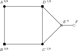
Figure 1: We show in Example 1 that $T:=\{A,B,C,D,E\}$ does not satisfy the assumptions of Theorem 4, but is a trapping subgraph with positive probability by Theorems 2 and 3. The numbers indicated in superscript of vertices represent the limit proportions of visits to these vertices if $x(n)$ were to converge to the equilibrium $x$ in the example. In this case the walk would asymptotically spend most of the time in the bipartite subgraph $S:=V_{1}\cup V_{2}$, where $V_{1}:=\{A,C\}$, $V_{2}:=\{B,D\}$, evenly divided between partitions $V_{1}$ and $V_{2}$, and vertex $E$ would be seldom visited, of the order of $\sqrt{n}$ times at time $n$.

Then, for any $x\in\Sigma$ and any neighborhood $\mathcal{N}(x)$ of $x$ in $\Sigma$, there exist random variables $y\in\mathcal{N}(x)$ and $C_{j}>0$, $j\in\partial S$ such that, with positive probability: [(iii)]

VRRW eventually localizes on $T$, that is, $\mathcal{R}=T$,

$Z_{n}(i)/n\longrightarrow_{n\to\infty}y_{i}$ for all $i\in S$,

$Z_{n}(j)\sim_{n\to\infty}C_{j}n^{r_{d}\sum_{i\sim j}a_{i,j}y_{i}/a_{S}}$ for all $j\in\partial S$.

Theorem 4 is proved in Section 2.2.3. We provide in Example 1 (illustrated in Figure 1) a counterexample showing that Theorem 3 is stronger, even in the case $a=(\mathbh{1}_{i\sim j})_{i,j\in G}$.

Third, which conditions on the graph and on the reinforcement matrix $a$ do ensure the existence of at least one strictly stable equilibrium $x\in\mathcal{E}_{s}$, thus implying localization with positive probability on $T(x)$? First note that, trivially, this does not always occur, for instance, on $\mathbb{Z}$ when $\phi(n):=a_{\{n,n+1\}}$ is strictly monotone, in which case we believe the walk to be transient.

In the case $a=(\mathbh{1}_{i\sim j})_{i,j\in G}$, Volkov volkov proposed the following result, using an iterative construction on subsets of the graph.

Proposition 2 ((Volkov volkov ))

Assume that $a=(\mathbh{1}_{i\sim j})_{i,j\in G}$, and that $(G,\sim)$ does not contain loops. Then, under either of the following conditions, there exists at least one strongly trapping subset: [(C)]

$(G,\sim)$ does not contain triangles;

$(G,\sim)$ is of bounded degree;

the size of any complete subgraph is uniformly bounded by some number $K$.

Start, for some $d\geq 2$, with any complete $d$-partite subgraph $(S,\sim)$ of $G$ with partitions $V_{1},\ldots,V_{d}$ (e.g., a pair of connected vertices, $d=2$). Let $x\in\partial S$, $S=V_{1}\cup\cdots\cup V_{d}$: [(3)]

First assume that $x\sim V_{p}$ for all $1\leq p\leq d$. Then, for all $1\leq p\leq d$, let $j_{p}\in V_{p}$ be such that $x\sim j_{p}$; iterate the procedure with the subgraph $\bigcup_{1\leq p\leq d}\{j_{p}\}\cup\{x\}$, which is a clique, and thus a complete $(d+1)$-partite subgraph.

Now assume there exists $p$ such that $x\not\sim V_{p}$, with $\partial\{x\}\supseteq S\setminus V_{p}$. Then we iterate the procedure with the complete $d$-partite subgraph $S\cup\{x\}$ with partitions $V_{1},\ldots,V_{p}\cup\{x\},\ldots,V_{d}$.

Otherwise we keep the same subgraph $S$ and try another $x\in\partial S$.

The construction eventually stops if (A), (B) or (C) holds. When it does, that is, when $S$ has remained unchanged for all $x\in\partial S$, then $T=S\cup\partial S$ is a strongly trapping subgraph in the sense of Definition 1.

Using a similar technique, we can obtain the following necessary condition for the existence of a strongly trapping subset in the case of general reinforcement matrices $a$, when the graph does not contain triangles or loops. Let us first introduce some notation. Let $c$ be the distance on $E(G)$ edges of $G$ defined as follows: for all $e$, $e^{\prime}\in E(G)$, let $c(e,e^{\prime})$ be the minimum number of edges necessary to connect $e$ to $e^{\prime}$ plus one ($0$ if $e=e^{\prime}$, and $1$ if $e\sim e^{\prime}$). For all $e=\{i,j\}$, let $\mathcal{C}(2,e)$ be the set of maximal complete $2$-partite subgraphs $S\subseteq G$ such that $i,j\in S$ and, for all $k,l\in S$ with $k\sim l$, $a_{k,l}=a_{i,j}$.

Proposition 3

Assume the graph does not contain triangles nor loops. If, for some $e\in E(G)$,

$$\min_{S\in\mathcal{C}(2,e)}\max_{k\in S,l\in\partial S}a_{k,l}\leq a_{e},$$ (9)

then there exists at least one strongly trapping subset.

Note that (9) holds if

$$\max_{c(e,e^{\prime})\leq 2}a_{e^{\prime}}\leq a_{e}.$$

Remark 3.

If, for all $e\in E(G)$, (9) does not hold, then there exists, for all $e\in E(G)$, an infinite sequence of edges $(e_{n})_{n\in\mathbb{N}_{0}}$ such that $e_{0}=e$, $e_{n}\sim e_{n+1}$ and, for all $n\in\mathbb{N}$, $a_{e_{n}}\leq a_{e_{n+1}}$ and $a_{e_{n}}<a_{e_{n+2}}$. However, even in this case, there can exist a strictly stable equilibrium $x\in\mathcal{E}_{s}$ (but no strongly trapping subset).

Proof of Proposition 3 By assumption, there exist $e=\{i,j\}$ and a maximal complete $2$-partite subgraph $S\subseteq G$ containing $i$ and $j$, with partitions $V_{1}$ and $V_{2}$, and satisfying conditions (a), (b) and (c)(i) of Definition 1. For all $k\in\partial S$, $k$ is adjacent to at most one of two partitions, say, $V_{1}$, since otherwise $G$ would contain a triangle; if $k$ were adjacent to all vertices in $V_{1}$, then it would be in $V_{2}$, since $S$ is assumed maximal. Hence, (c)(ii) holds as well, and $S$ is a strongly trapping subset.

When the graph contains triangles, the property outlined in Remark 3, that is, the existence of an infinite sequence of edges with increasing labels when there is no strongly trapping subset, does not hold anymore. The maximum of the Lyapounov function on a complete subgraph with more than two vertices takes a nontrivial form, which can lead to counterintuitive behavior.

We show, for instance, in Example 2 a case where the reinforcement matrix $a$ has a strict global maximum at a certain edge, but where, however, there is no stable equilibrium at all. We believe the walk to be transient in this example.

Example 1.

Let us show, in the case $a=(\mathbh{1}_{i\sim j})_{i,j\in G}$, that Theorem 3 is stronger than Theorem 4. Consider a graph $G$ on six vertices $A$, $B$, $C$, $D$, $E$ and $F$, with a neighborhood relation $\sim$ defined as follows (see Figure 1): $A\sim B\sim C\sim D\sim A$, $C\sim E\sim D$ and $E\sim F$ (recall that the graph $G$ is symmetric). Let $x=(x_{A},x_{B},x_{C},x_{D},x_{E},x_{F}):=(3/8,3/8,1/8,1/8,0,0)$, then $S(x)=\{A,B,C,D\}$ and $\partial S(x)=\{E\}$. Also, $x$ is an equilibrium of (6), (P)_S(x) is satisfied with $V_{1}=\{A,C\}$, $V_{2}=\{B,D\}$, and $N_{E}(x)=1/4<H(x)=1/2$, which implies that $x$ is a strictly stable equilibrium by Theorem 2, hence subsequently by Theorem 3 that $\mathcal{R}=T(x)$ with positive probability.

Now let us prove by contradiction that $T(x)$ with such $x$ does not satisfy the assumptions of Theorem 4 above. Indeed, if $T(x)=S\cup\partial S$, then $S\subseteq\{A,B,C,D\}$ since, otherwise, $F$ would belong to $T(x)$. Now the condition that, for all $i\in\partial S$, $\exists p\in\{1,\ldots,d\}$ and $j\in S\setminus V_{p}$ such that $i\not\sim V_{p}\cup\{j\}$ implies, in particular, that a vertex in $\partial S$ is not connected to at least two other vertices in $S$, so that $i\in\partial S$ cannot be $A$, $B$, $C$ or $D$, which are connected to all other but one vertex in $\{A,B,C,D\}$. Hence, $S=\{A,B,C,D\}$, but then $i:=E$ is connected to both partitions of $S$, and does not satisfy the condition mentioned in the last sentence, bringing a contradiction.

Example 2.

Let us first study the case of a triangle $(G,\sim)$, $G:=\{0,1,2\}$, $0\sim 1\sim 2\sim 0$, with reinforcement coefficients $a:=a_{0,1}$, $b:=a_{1,2}$, $c:=a_{0,2}>0$.

If $a<b+c$, then the equilibrium $x=(x_{0},x_{1},x_{2})=(1/2,1/2,0)$ is not stable, since $N_{2}(x)=(b+c)/2>H(x)=a/2$. Hence, if we assume that

$$a<b+c,\qquad b<a+c,\qquad c<a+b,$$ (10)

then a stable equilibrium has to belong to the interior of the simplex $\Delta$. A simple calculation shows that there is only one such equilibrium:

$$x=(x_{0},x_{1},x_{2}):=\biggl{(}\frac{c(a+b-c)}{\delta},\frac{b(a+c-b)}{\delta},\frac{a(b+c-a)}{\delta}\biggr{)},$$

where

$$\delta:=(a+b+c)^{2}-2(a^{2}+b^{2}+c^{2});$$

$\delta\,{>}\,0$, which can be shown by adding up inequalities $(b-a)^{2}\,{\leq}\,c^{2}$, $(c-a)^{2}\,{\leq}\,b^{2}$ and $(c-b)^{2}\,{\leq}\,a^{2}$. Then $H(x)=2abc/\delta$.

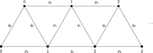
Figure 2: On the infinite graph on the figure, with reinforcement coefficient sequences $(p_{n})_{n\geq 0}$ strictly decreasing and $(q_{n})_{n\geq 0}$ strictly increasing, we show in Example 2 that, even if $p_{0}=\sup_{n\geq 0}p_{n}>\sup_{n\geq 0}q_{n}$, we can choose these sequences in such a way that there is no stable equilibrium in $\Delta$, and therefore no trapping subgraph.

Let $\mathbb{N}:=\mathbb{Z}_{+}$. Let us now consider the following graph $(G,\sim)$ with vertices $G:=\{\underline{i},\overline{i},i\in\mathbb{N}\}$ and adjacency $\underline{i}\sim\underline{i+1}$, $\overline{i}\sim\overline{i+1}$, $\underline{i}\sim\overline{i}$ and $\overline{i}\sim\underline{i+1}$, for all $i\in\mathbb{N}$, as drawn in Figure 2.

Fix $\varepsilon,\eta,p,q>0$, $\mu\in(0,1)$, which will be chosen later. Let, for all $n\in\mathbb{N}$,

$$p_{n}:=p\prod_{k=0}^{n-1}(1-\mu^{k}\varepsilon),\qquad q_{n}:=q\prod_{k=0}^{n-1}(1+\mu^{k}\eta).$$ (11)

Note that, for all $n\in\mathbb{N}$,

$$p\biggl{(}1-\frac{\varepsilon}{1-\mu}\biggr{)}\leq p_{n}\leq p,\qquad q\leq q_{n}\leq qe^{{\eta}/{(1-\mu)}}.$$

Now assume that the reinforcement matrix $(a_{k,l})_{k,l\in G}$ is defined as follows, depending on $(p_{n})_{n\in\mathbb{N}}$ and $(q_{n})_{n\in\mathbb{N}}$, for all $i\in\mathbb{N}$:

$$a_{\underline{2i},\underline{2i+1}} := p_{2i},\qquad a_{\overline{2i+1},\overline{2(i+1)}}:=p_{2(i+1)},$$

$$a_{\overline{2i},\overline{2i+1}} \hskip 3.0pt= a_{\underline{2i+1},\underline{2(i+1)}}:=q_{2i+1}$$

$$a_{\underline{2i},\overline{2i}} \hskip 3.0pt= a_{\overline{2i},\underline{2i+1}}:=q_{2i}$$

$$a_{\underline{2i+1},\overline{2i+1}} := p_{2i+1}$$

$$a_{\overline{2i+1},\underline{2(i+1)}} := q_{2i+1}.$$

Let $x\in\Delta$ be a stable equilibrium of (6). Then, by Theorem 1, (P)_S(x) holds, so that $S(x)$ consists of two vertices or a triangle [it cannot be made of four vertices, because of (P)_S(x)(c)]. Assume

$$p<2q,\qquad\eta qe^{{\eta}/{(1-\mu)}}<p\biggl{(}1-\frac{\varepsilon}{1-\mu}\biggr{)}.$$ (12)

Then, for all $i\in\mathbb{N}$,

$$p_{i}<2q_{i},\qquad p_{i+1}<q_{i}+q_{i+1},\qquad q_{i+1}<q_{i}+p_{i+1},$$

so that $S(x)$ has to be a triangle.

Assume $S(x):=\{\underline{2i},\overline{2i},\underline{2i+1}\}$ for some $i\in\mathbb{N}$; the argument is similar in other cases. Then

$$x_{\overline{2i+1}}=\frac{H(x)}{2q_{i}},\qquad x_{\overline{2i}}=\frac{H(x)}{2q_{i}^{2}}(2q_{i}-p_{i}),\qquad x_{\underline{2i+1}}=\frac{H(x)}{2q_{i}},$$

and

$$N_{\underline{2i}}(x)=q_{i}x_{\overline{2i}}+p_{i}x_{\underline{2i+1}}=H(x),$$

and, therefore,

$$N_{\overline{2i+1}}(x) = q_{i+1}x_{\overline{2i}}+p_{i+1}x_{\underline{2i+1}}$$

$$= H(x)+\frac{H(x)}{2q_{i}^{2}}[(q_{i+1}-q_{i})(2q_{i}-p_{i})+(p_{i+1}-p_{i})q_{i}]$$

$$= H(x)+\frac{H(x)}{2q_{i}^{2}}\mu^{i}[\eta q_{i}(2q_{i}-p_{i})-\varepsilon p_{i}q_{i}]>H(x)$$

if

$$\eta>\varepsilon\frac{p}{2q-p},$$ (13)

using that $p/(2q-p)>p_{i}/(2q_{i}-p_{i})$ for all $i\in\mathbb{N}$.

Hence, $x$ is not a stable equilibrium, which leads to a contradiction.

2 Introduction to the proofs

2.1 Notation

We let $\mathbb{N}:=\mathbb{Z}_{+}$, $\mathbb{N}^{*}:=\mathbb{N}\setminus\{0\}$, $\mathbb{R}_{+}^{*}:=\mathbb{R}_{+}\setminus\{0\}$.

For all $y=(y_{i})_{i\in G}\in\mathbb{R}^{G}$ and for any finite subset $A$ of $G$, let

$$y_{A}:=\sum_{i\in A}y_{i}.$$

Given $r\in\mathbb{N}^{*}$, let $(\cdot,\cdot)$ (resp., $|\cdot|$, $\|\cdot\|_{\infty}$) be the scalar product (resp., the canonical norm, the infinity norm) on $\mathbb{R}^{r}$, defined by

$$(a,b)=\sum_{i=1}^{r}a_{i}b_{i},\qquad|a|=\sqrt{(a,a)},\qquad\|a\|_{\infty}:=\max_{1\leq i\leq r}|a_{i}|$$

if $a=(a_{1},\ldots,a_{r})$ and $b=(b_{1},\ldots,b_{r})$.

Given a real $r\times r$ matrix $M$ with real eigenvalues, we let $\operatorname{\mathsf{Sp}}(M)$ denote the set of eigenvalues of $M.$ When $M$ is symmetric we let $M[\cdot]$ denote the quadratic form associated to $M$, defined by $M[a]=(Ma,a)$ for all $a\in\mathbb{R}^{r}$.

Given $y_{1},\ldots,y_{r}$, we let $\operatorname{\mathsf{Diag}}(y_{1},\ldots,y_{r})$ be the diagonal $r\times r$ matrix of diagonal terms $y_{1},\ldots,y_{r}$.

For all $u,v\in\mathbb{R}$, we write $u=\Box(v)$ if $|u|\leq v$. Given two (random) sequences $(u_{n})_{n\geq k}$ and $(v_{n})_{n\geq k}$ taking values in $\mathbb{R}$, we write $u_{n}\equiv v_{n}$ if $u_{n}-v_{n}$ converges a.s., and $u_{n}\sim_{n\to\infty}v_{n}$ iff $u_{n}/v_{n}\to_{n\to\infty}1$, with the convention that $0/0=1$.

Let $\mathsf{Cst}(a_{1},a_{2},\ldots,a_{p})$ denote a positive constant depending only on $a_{1},a_{2},\allowbreak\ldots,a_{p}$, and let $\mathsf{Cst}$ denote a universal positive constant.

2.2 Proof of Theorems 1, 2 and 4

Theorems 1 and 2 are a consequence of the more general three following Lemmas 1, 2 and 3 below.

2.2.1 Lemmas 1, 2 and 3, and proof of Theorem 1

By the following Lemma 1, if an equilibrium $x\in\Delta$ is stable, then the eigenvalues of $[a_{i,j}-2H(x)]_{i,j\in S(x)}$, which depend only on $a$, $S(x)$ and $H(x)$, are nonpositive. This property will subsequently imply (P)_S(x), by Lemmas 2 and 3.

Lemma 1

Let $x=(x_{i})_{i\in G}\in\Delta$ be an equilibrium. Then:

1. [(a)]

2. $DF(x)$ has real eigenvalues.

3. The three following assertions are equivalent:

   1. [(iii)]

   2. $x$ is stable,

   3. $\max\operatorname{\mathsf{Sp}}(DF(x))\leq 0$,

   4. $\max(\operatorname{\mathsf{Sp}}([a_{i,j}-2H(x)]_{i,j\in S(x)})\cup\{N_{i}(x)-H(x),i\in\partial S(x)\})\leq 0$.

4. If $x$ is stable, then it is feasible.

Lemma 2 yields an algebraically simpler characterization of assertion (P)_S for $S\subseteq G$; recall that, given subsets $S$ and $R$ of $G$, $\partial_{S}R$, defined in Section 1, is the outer boundary of $R$ inside $S$.

Lemma 2

The statement (P)_S is equivalent to

1. [$\mathrm{(P)}_{S}^{\prime}$]

2. If $j,k\in S$ are such that $j\not\sim k$, then, for all $i\in S$, $a_{i,j}=a_{i,k}$ (so that $\partial_{S}\{j\}=\partial_{S}\{k\}$ in particular).

Lemma 3 states that (P)_S(x) holds if the eigenvalues of $[a_{i,j}-2H(x)]_{i,j\in S(x)}$ are nonpositive, with equivalence if $a=(\mathbh{1}_{i\sim j})_{i,j\in G}$.

Lemma 3

Let $x=(x_{i})_{i\in G}\in\Delta$ be a feasible equilibrium. Then

$$\max\operatorname{\mathsf{Sp}}\bigl{(}[a_{i,j}-2H(x)]_{i,j\in S(x)}\bigr{)}\leq 0\quad\Longrightarrow\quad\mbox{{(P)}}_{S(x)}^{\prime}.$$

If, for some $c>0$, $a_{i,j}=c\mathbh{1}_{i\sim j}$ for all $i,j\in S(x)$, then the above implication is an equivalence.

Lemmas 1, 2 and 3 are proved, respectively, in Sections 3.1, 3.2 and 3.3. They obviously imply Theorem 1.

2.2.2 Proof of Theorem 2

Suppose $a=(\mathbh{1}_{i\sim j})_{i,j\in G}$, and let $x\in\Delta$.

First assume that $(S(x),\sim)$ contains no loop. If $x$ is a stable equilibrium, then (P)_S(x) and, thus, (i) holds by Theorem 1; let $V_{k}$, $1\leq k\leq d$ be the partitions of $S(x)$. Then $d\geq 2$ [otherwise $H(x)=0$ and $x$ is not feasible, thus not stable by Lemma 1] and, for all $1\leq k\leq d$, $j\in V_{k}$,

$$v_{k}:=\sum_{i\in V_{k}}x_{i}=1-N_{j}(x)=1-H(x),$$

so that $v_{k}=1/d$ (since $\sum_{k}v_{k}=1$) and $H(x)=1-1/d$, and, subsequently, (ii)–(iii) hold by Lemma 1. Conversely, assume (i)–(iii) hold; then $N_{i}(x)=1-1/d$ for all $i\in S(x)$, so that $H(x)=\sum_{i\in S(x)}x_{i}N_{i}(x)=1-1/d$ and $x$ is a feasible equilibrium. Now (i) implies (P)_S(x) and thus (P)${}_{S(x)}^{\prime}$ by Lemma 2. Hence, using Lemmas 1 and 3, $x$ is a stable equilibrium.

Now assume on the contrary that $(S(x),\sim)$ contains one loop $i\sim i$. If $x$ is a stable equilibrium, then (P)_S(x) again holds by Theorem 1: (P)_S(x)(b) implies $N_{i}(x)=1=H(x)$ ($x$ equilibrium). Hence, for all $j\in S(x)$, $N_{j}(x)=1$ and $j\sim k$ for all $k\in S(x)$, that is, $(S(x),\sim)$ is a clique of loops. Conversely, if $(S(x),\sim)$ is a clique of loops, then (P)_S(x) obviously holds so that, by Lemmas 1 and 3, $x$ is stable [since $H(x)=1$, then $N_{i}(x)\leq H(x)$ for all $i\in G$].

2.2.3 Proof of Theorem 4

First observe that

$$\Sigma=\mathcal{S}(S)\cap\mathcal{E}_{s}.$$

Indeed, the proof of Theorem 2 implies that $\Sigma\supseteq\mathcal{S}(S)\cap\mathcal{E}_{s}$ and, conversely, that if $x\in\Sigma$, then $x$ is a equilibrium and, by (c)(ii), for all $j\in\partial S(x)$, $N_{j}(x)<H(x)$ [$=a_{S}(1-1/d)$ if $(S(x),\sim)$ contains no loops, $=a_{S}$ otherwise], using assumptions (a)–(b) and (c)(ii) or the second part of (c)^′. Also, (P)_S(x) holds by (c) or (c)^′, and, therefore, $x$ is strictly stable by Lemmas 1–3. The rest of the proof follows from Theorem 3.

2.3 Proof of Theorem 3

First, we provide in Lemma 4 a rigorous mathematical setting for the stochastic approximation of the density of occupation of the VRRW $x(n)$ by solutions of the ordinary differential equation (6) on a finite graph $G$, heuristically justified in Section 1 [see (4)]. Second, we make use of this technique and of an entropy function originally introduced in losert to study the VRRW on the finite subgraph $T(x)$ when its density of occupation is in the neighborhood of a strictly stable equilibrium $x$, in Lemmas 5–10. Third, we focus again on a general graph $G$—possibly infinite—and prove in Proposition 4, assuming again that the density of occupation is in the neighborhood of an element $x\in\mathcal{E}_{s}$, that the walk eventually localizes in $T(x)$ with lower bounded probability.

In the first step, we make use of a technique originally introduced by Métivier and Priouret in 1987 metivier and adapted by Benaïm benaim1 in the context of vertex reinforcement when the graph is complete (Hypothesis 3.1 in benaim1 ). In Sections 4.1–4.3, we generalize it and show that a certain quantity $z(n)$, depending only on $a$, $x(n)$, $X_{n}$ and $n$ and defined in (36), satisfies the recursion (37):

$$z(n+1)=z(n)+\frac{1}{n+n_{0}+1}\frac{F(z(n))}{H(x(n))}+\varepsilon_{n+1}+r_{n+1},$$

where $\mathbb{E}(\varepsilon_{n+1}|\mathcal{F}_{n})=0$. The following Lemma 4, proved in Section 4.3, provides upper bounds on the infinity norms of $\varepsilon_{n+1}$, $r_{n+1}$ and $z(n)-x(n)$, and on the conditional variances of $(\varepsilon_{n+1})_{i}$, $i\in G$.

More precisely, let us break down the set of vertices of $G$ as $G=S\cup\partial S$, where $(S,\sim)$ is finite, connected and not a singleton unless it is a loop. Let, for all $\alpha\in\mathbb{R}_{+}\setminus\{0\}$,

$$\Lambda_{\alpha}:=\{x=(x_{j})_{j\in G}\in\Delta\mbox{ s.t. }x_{j}\geq\alpha\mbox{ for all }j\in S\}.$$ (14)

Lemma 4

For all $n\geq\mathsf{Cst}(\alpha)$ and $i\in G$, if $x(n)\in\Lambda_{\alpha}$, then

$$\mbox{{(a)}}\quad\!\!\|\varepsilon_{n+1}\|_{\infty} \leq \frac{\mathsf{Cst}(\alpha,a,|G|)}{n+n_{0}},\qquad\mbox{{(b)}}\quad\!\!\mathbb{E}((\varepsilon_{n+1})_{i}^{2}|\mathcal{F}_{n})\leq\frac{\mathsf{Cst}(\alpha,a,|G|)x(n)_{i}}{(n+n_{0})^{2}},$$

$$\mbox{{(c)}}\quad\!\!\|r_{n+1}\|_{\infty} \leq \frac{\mathsf{Cst}(\alpha,a,|G|)}{(n+n_{0})^{2}},\qquad\mbox{{(d)}}\quad\!\!\|z(n)-x(n)\|_{\infty}\leq\frac{\mathsf{Cst}(\alpha,a,|G|)}{n+n_{0}}.$$

Note that if $G$ were a complete $d$-partite finite graph for some $d\geq 1$ or, more generally, if $G$ were without loop and, for all $i,j\in G$ with $i\sim j$, $\{i,j\}\cup\partial\{i,j\}=G$, then the constants in the inequalities of Lemma 4 would not depend on $\alpha>0$ and, as a consequence, the stochastic approximation of $z(n)$ by (6) would hold uniformly a.s. Indeed, for all $n\in\mathbb{N}$, by the pigeonhole principle, there exists at least one edge $\{i,j\}$ $i,j\in G$, $i\sim j$, on which the walk has spent more than $n/|G|^{2}$ times, so that $x(n)_{i}\wedge x(n)_{j}\geq\frac{1}{|G|^{2}}\frac{n}{n+n_{0}}$ and, under the assumption on $G$, Lemma 4 with $S:=\{i,j\}$ would yield the claim.

In the second step, we define an entropy function $V_{q}(\cdot)$, measuring a “distance” between $q$ and an arbitrary point [as can be seen by (15) below], originally introduced by Losert and Akin in 1983 in losert in the study of the deterministic Fisher–Wright–Haldane population genetics model, and to our knowledge so far only used for the analysis of deterministic replicator dynamics. Note that it is not mathematically a distance, however, since it does not satisfy the triangle inequality in general.

In the following, until after the statement Lemma 10—and, in particular, in Lemmas 5–10—we assume that $x\in\mathcal{E}_{s}$ and $G=T(x)=S(x)\cup\partial S(x)$; this choice will be justified later in the proof. Note that if $q\in\mathcal{N}(x)\cap\mathcal{E}_{s}$, where $\mathcal{N}(x)$ is an adequately chosen neighborhood of $x$, then $q\in\mathcal{S}(S(x))$ since $x\in\mathcal{E}_{s}$, so that $T(q)=T(x)$. Set $S:=S(x)$, $T:=T(x)$, and $\mathcal{S}:=\mathcal{S}(S(x))$ for simplicity.

Lemmas 5 and 6 below will imply that, given any stable equilibrium $q\in\mathcal{N}(x)\cap\mathcal{E}_{s}$ as a reference point, $V_{q}(z(n))$ decreases in average when $z(n)$ is close enough to $x$. Therefore, martingale estimates will enable us to prove in Lemma 7 that, starting in the neighborhood of $x$, $x(n)$ remains close to $x$ with large probability if $n$ is large, and converges to one of the strictly stable equilibria in this neighborhood.

For all $q=(q_{i})_{i\in G}\in\mathcal{S}$ and $y\in\mathbb{R}^{G}$, let

$$V_{q}(y):=\cases{\displaystyle-\sum_{i\in S}q_{i}\log(y_{i}/q_{i})+2y_{\partial S},&\quad if $y_{i}>0$, $\forall i\in S$,\cr\infty,&\quad otherwise.}$$

Let, for all $q\in\mathcal{S}$ and $r>0$,

$$B_{V_{q}}(r):=\{y\in\Delta\mbox{ s.t. }V_{q}(y)<r\},\qquad B_{\infty}(q,r):=\{y\in\Delta\mbox{ s.t. }\|y-q\|_{\infty}<r\}.$$

Then, we will prove in Section 4.4 that, for all $q\in\mathcal{S}$, there exist increasing continuous functions $u_{1,q}$, $u_{2,q}\dvtx\mathbb{R}_{+}\longrightarrow\mathbb{R}_{+}$ such that $u_{1,q}(0)=u_{2,q}(0)=0$ and, for all $r>0$,

$$B_{\infty}(q,u_{1,q}(r))\subseteq B_{V_{q}}(r)\subseteq B_{\infty}(q,u_{2,q}(r)).$$ (15)

Let, for all $q,z\in\mathbb{R}^{G}$,

$$I_{q}(z):=-\sum_{i\in S}q_{i}[N_{i}(z)-H(z)]+2\sum_{i\in\partial S}z_{i}[N_{i}(z)-H(z)].$$ (16)

The following Lemma 5, also proved in Section 4.4, provides the stochastic approximation equation for $V_{q}(z(n))$, $q\in\mathcal{S}\cap\mathcal{E}_{s}$; we make use of notation $u=\Box(v)\iff|u|\leq v$, introduced in Section 2.1.

Lemma 5

Let $q\in\mathcal{S}\cap\mathcal{E}_{s}$. There exist an adapted process $(\zeta_{n})_{n\in\mathbb{N}}$ (not depending on $q$ and $a$), and constants $n_{1}$ and $\varepsilon$ (depending only on $q$ and $a$) such that, if $n\geq n_{1}$ and $x(n)\in B_{V_{q}}(\varepsilon)$, then $V_{q}(z(n))<\infty$, $V_{q}(z(n+1))<\infty$, $\mathbb{E}(\zeta_{n+1}|\mathcal{F}_{n})=0$ and

$$V_{q}\bigl{(}z(n+1)\bigr{)} = V_{q}(z(n))+\frac{I_{q}(x(n))}{(n+n_{0}+1)H(x(n))}$$

$${}-(q,\zeta_{n+1})+2(\varepsilon_{n+1})_{\partial S}+\Box\biggl{(}\frac{\mathsf{Cst}(q,a)}{(n+n_{0})^{2}}\biggr{)}.$$

Lemma 6, proved in Section 3.4, provides estimates of the Lyapounov function $H$, and of $I_{\cdot}(\cdot)$, in the neighborhood of a strictly stable equilibrium. It will not only be useful in the proof of Lemma 7, stating convergence of $x(n)$ with large probability, but also for Lemma 8 on the rate of this convergence.

Lemma 6

There exists a neighborhood $\mathcal{N}(x)$ of $x$ in $\Delta$ such that, for all $q\in\mathcal{N}(x)\cap\mathcal{E}_{s}$, $y\in\mathcal{N}(x)$,

$$\mbox{{(a)}}\quad\mathsf{Cst}(x,a)J(y)\leq H(q)-H(y)\leq\mathsf{Cst}(x,a)J(y),$$ (18)

$$\mbox{{(b)}}\quad{-}[H(q)-H(y)+\mathsf{Cst}(x,a)y_{\partial S}]$$

(19)

$$\hphantom{\mbox{{(b)}}\quad}\qquad\leq I_{q}(y)\leq-[H(q)-H(y)+\mathsf{Cst}(x,a)y_{\partial S}]\leq 0.$$

Remark 4.

Lemma 6 implies that $y\in\mathcal{N}(x)$ is an equilibrium iff $H(y)=H(x)$. Also note that the maximality of $H$ at $x\in\mathcal{E}_{s}$ is not global in general. For instance, in the counterexample at the end of Section 1, $x:=(3/8,3/8,1/8,1/8,0)\in\mathcal{E}_{s}$, but, letting $y:=(0,0,1/3,1/3,1/3)$, $H(y)=2/3>H(x)=1/2$.

The proof of Lemma 7 is shown in Section 5.1. A key point in its proof is that the martingale term $-(q,\zeta_{n+1})+2(\varepsilon_{n+1})_{\partial S}$, in Lemma 5, is a linear function of $\zeta_{n+1}$ and $\varepsilon_{n+1}$ which do not depend on $q$, so that the two corresponding convergence results of these martingales will apply from any reference point $q\in\mathcal{E}_{s}\cap\mathcal{N}(x)$. It will enable us to prove that, if $r$ is a accumulation point of $x(n)$, then $V_{r}(x(n))$ a.s. converges to $0$ if $r\in\mathcal{N}(x)$ although $r$ is random.

Lemma 7

There exist $\varepsilon_{0}:=\mathsf{Cst}(x,a)$ and $n_{1}:=\mathsf{Cst}(x,a)$ such that, if for some $\varepsilon\leq\varepsilon_{0}$ and $n\geq n_{1}$, $x(n)\in B_{V_{x}}(\varepsilon/2)$, then

$$\mathbb{P}\bigl{(}\mathcal{L}(B_{V_{x}}(\varepsilon))|\mathcal{F}_{n}\bigr{)}\geq 1-\exp\bigl{(}-\varepsilon^{2}\mathsf{Cst}(x,a)(n+n_{0})\bigr{)}.$$

Next, we provide in Lemma 8 some information on the rate of convergence of $x(n)$ to $x(\infty)$, which will be necessary for the asymptotic estimates on the frontier $\mathcal{A}_{\partial}(x(\infty))$ in Lemma 10.

Lemma 8

There exist $\varepsilon$, $\nu:=\mathsf{Cst}(x,a)$ such that, a.s. on $\mathcal{L}(B_{V_{x}}(\varepsilon))$,

$$\lim_{n\to\infty}\bigl{(}x(n)-x(\infty)\bigr{)}n^{\nu}=0.$$

The proof of Lemma 8, given in Section 5.2, starts with a preliminary estimate of the rate of convergence of $H(x(n))$ to $H(x(\infty))$. To this end, we make use of Lemma 9 below, giving the stochastic approximation equation of $H(z(n))$. It implies, together with Lemma 6(a), that the expected value of $H(z(n+1))-H(z(n))$ is at least $\mathsf{Cst}(x,a)(H(x)-H(z(n))$, so that we can then estimate the rate of $H(x(n))$ to $H(x)$ by a one-dimensional technique.

Finally, this estimate implies similar ones for the convergence of $J(x(n))$ and $I_{x(\infty)}(x(n))$ to $0$ by Lemma 6, so that we conclude using entropy estimates for the rate of convergence of $V_{x(\infty)}(z(n))$, using again that only two martingales estimates are necessary, given the linearity of the perturbation in (5) with respect to the reference point $q\in\mathcal{E}_{s}\cap\mathcal{N}(x)$.

Lemma 9

For all $n\in\mathbb{N}$,

$$H\bigl{(}z(n+1)\bigr{)}-H(z(n))=\frac{1}{n+n_{0}+1}\frac{J(z(n))}{H(x(n))}+\xi_{n+1}+s_{n+1},$$ (20)

where $\mathbb{E}(\xi_{n+1}|\mathcal{F}_{n})=0$ and, if for some $\alpha>0$, $x(n)\in\Lambda_{\alpha}$ and $n\geq\mathsf{Cst}(\alpha)$, then

$$(1)\quad\|\xi_{n+1}\|_{\infty}\leq\frac{\mathsf{Cst}(\alpha,a,|G|)}{n+n_{0}},\qquad(2)\quad\|s_{n+1}\|_{\infty}\leq\frac{\mathsf{Cst}(\alpha,a,|G|)}{(n+n_{0})^{2}}.$$

Lemma 9 is proved in Section 4.5.

Lemma 10 yields the asymptotic behavior on the border sites $\partial S$. This behavior is similar to the one one would obtain without perturbation [i.e., with $(\varepsilon_{n})_{n\in\mathbb{N}^{*}}=0$ in (37)]. Indeed, if $i\in\partial S$, then $N_{i}(x)-H(x)<0$ is the eigenvalue of the Jacobian matrix of (6) in the direction $(\delta_{i,j})_{j\in G}$ (see the proof of Lemma 1), and the renormalization in time is approximately in $H(x)^{-1}\log n$ [see equation (37)], so that the replicator equation (6) would predict that $i\in\partial S$ is visited of the order of $n^{N_{i}(x)/H(x)}$ times at time $n$. This similarity with the noiseless case is due to the fact that the perturbation $(\varepsilon_{n})_{n\in\mathbb{N}^{*}}$ is weak near the boundary [see Lemma 4(b)].

Lemma 10

There exists $\varepsilon:=\mathsf{Cst}(x,a)$ such that, a.s. on $\mathcal{L}(B_{V_{x}}(\varepsilon))$, $\mathcal{A}_{\partial}(x(\infty))$ occurs a.s.

The proof of Lemma 10, given in Section 5.3, makes use of a martingale technique developed in tarres , Section 3.1, and in limtar in the context of strong edge reinforcement. We could have shown Lemma 10 by a thorough study of the border sites coordinates of the stochastic approximation equation (37), but it would lead to a significantly longer—and less intuitive—proof.

Now we do not assume anymore that $G=T(x)$ for some $x\in\Delta$, in other words, we let the graph $(G,\sim)$ be arbitrary, possibly infinite.

Let, for all $n,k\in\mathbb{N}\cup\{\infty\}$, $n\geq k$, $\mathcal{R}_{n,k}$ be the range of the vertex-reinforced random walk between times $n$ and $k$, that is,

$$\mathcal{R}_{n,k}:=\{i\in G\mbox{ s.t. }X_{j}=i\mbox{ for some }j\in[n,k]\};$$

note that, for all $n\in\mathbb{N}$, $\mathcal{R}\subseteq\mathcal{R}_{n,\infty}$.

Proposition 4

Let $x\in\mathcal{E}_{s}$. There exists $\varepsilon:=\mathsf{Cst}(x,a)$ such that, for all $n\geq\mathsf{Cst}(x,a)$, if $X_{n}\in T(x)$ and $x(n)\in B_{V_{x}}(\varepsilon/2)$, then

$$\mathbb{P}\bigl{(}\{\mathcal{R}_{n,\infty}=T(x)\}\cap\mathcal{L}(B_{V_{x}}(\varepsilon))\cap\mathcal{A}_{\partial}(y(\infty))|\mathcal{F}_{n}\bigr{)}>0.$$

Moreover, the rate of convergence is at least reciprocally polynomial, that is, there exists $\nu:=\mathsf{Cst}(x,a)$ such that, a.s. on $\mathcal{L}(B_{V_{x}}(\varepsilon))$,

$$\lim_{k\to\infty}\bigl{(}y(k)-y(\infty)\bigr{)}k^{\nu}=0.$$

Proposition 4 is proved in Section 5.4. It obviously implies Theorem 3: indeed, given $U$ a neighborhood of $x$, there exists $\varepsilon>0$ such that $B_{V_{x}}(\varepsilon)\subseteq U$, and $X_{n}\in T(x)$ and $x(n)\in B_{V_{x}}(\varepsilon/2)$ occurs with positive probability if $n$ is large enough.

Observe that, if $G=T(x)$, then this Proposition 4 is a direct consequence of Lemmas 7, 8 and 10. The localization with positive probability in this subgraph $T(x)$ results from a Borel–Cantelli type argument: the probability to visit $\partial T(x)$ at time $n$ starting from $S(x)$ is, by Lemma 10, upper bounded by a term smaller than $n^{\alpha-2}$, where $\alpha\approx\max_{i\in\partial S}N_{i}(x)/H(x)<1$, and $\sum_{n\in\mathbb{N}}n^{\alpha-2}<\infty$. Technically, the proof is based on a comparison of the probability of arbitrary paths remaining in $T(x)$ for the VRRWs defined, respectively, on the graphs $T(x)$ and $G$.

2.4 Contents

Section 3 concerns the results on the deterministic replicator dynamics: Lemmas 1–3 and Lemma 6 are proved, respectively, in Sections 3.1–3.3 and 3.4.

Section 4 develops the framework relating the behavior of the vector of density of occupation $x(n)$ to the replicator equation (6): we write the stochastic approximation equation (37) in Section 4.1, establish in Section 4.2 some preliminary estimates on the underlying Markov Chain $M(x)$, prove Lemma 4 in Section 4.3, prove Lemmas 5 and 9 [stochastic approximation equations for $V_{q}(z(n))$ and $H(z(n))$] and inclusions (15) in Sections 4.4 and 4.5.

Section 5 is devoted to the proofs of the asymptotic results for the VRRW: Lemma 7 in Section 5.1 on the convergence of $x(n)$ with positive probability, Lemma 8 in Section 5.2 on the corresponding speed of convergence, Lemma 10 in Section 5.3 on the asymptotic behavior of the number of visits on the frontier of the trapping subset, and Proposition 4 in Section 5.4 on localization with positive probability in the trapping subsets.

Finally, we show in Appendix .5 a lemma on the remainder of square-bounded martingales, which is useful in the proofs of Lemma 8 and Proposition 1, whereas Appendix .6 is devoted to the proof of Proposition 1.

3 Results on the replicator dynamics

3.1 Proof of Lemma 1

Note that $DF(x)v=-H(x)v=0$ if $S(v)\cap T(x)=\varnothing$, so that it is sufficient to study the eigenvalues of $DF(x)$ on $\{v\in\mathbb{R}^{G}\mbox{ s.t. }S(v)\subseteq T(x)\}$; hence, we can assume that $G$ is finite [equal to $T(x)$] w.l.o.g.

Let $S:=S(x)$ for convenience. For all $i,j\in G$,

$$\frac{\partial F_{i}}{\partial x_{j}}=\cases{N_{i}(x)-H(x),&\quad if $x_{i}=0$ and $j=i$,\cr 0,&\quad if $x_{i}=0$ and $j\not=i$,\cr x_{i}[a_{i,j}-2H(x)],&\quad if $x_{i}\not=0$ and $x_{j}\not=0$,\cr x_{i}[a_{i,j}-2N_{j}(x)],&\quad if $x_{i}\not=0$ and $x_{j}=0$.}$$

Let us now consider matrix $DF(x)$ by taking the following order on the indices: we take first the indices $i,j\in G\setminus S$, and second the indices $i,j\in S$,

$$\pmatrix{\operatorname{\mathsf{Diag}}\bigl{(}N_{i}(x)-H(x)\bigr{)}_{i\in G\setminus S}&(0)\cr(*)&DB},$$

where

$$B=[a_{i,j}-2H(x)]_{i,j\in S},\qquad D=\operatorname{\mathsf{Diag}}(x_{i})_{i\in S}.$$

The matrix $DB$ is easily seen to be self-adjoint with respect to the scalar product $(u,v)_{D^{-1}}:=(D^{-1}u,v).$ Hence, $DB$ has real eigenvalues. This proves the first statement of the lemma.

Note that if we consider (6) as a differential equation on $\mathbb{R}^{G}$, then

$$(F(x),\mathbh{1})=\frac{d(x(t),\mathbh{1})}{dt}\bigg{|}_{t=0,x(0)=x}=-\bigl{(}(x,\mathbh{1})-1\bigr{)}H(x).$$

Therefore, if $x\in\Delta$ [which implies $(x,\mathbh{1})=1$], for all vector $u\in\mathbb{R}^{G}$,

$$(DF(x)u,\mathbh{1})=-H(x)(u,\mathbh{1}).$$ (21)

Hence, $p\dvtx u\mapsto(u,\mathbh{1})$ is an eigenvector of ${}^{t}DF(x)$ with eigenvalue $-H(x).$ This makes $-H(x)$ an eigenvalue of $DF(x)$ and, more precisely,

$$\operatorname{\mathsf{Sp}}(DF(x))=\{-H(x)\}\cup\operatorname{\mathsf{Sp}}(DF(x)|_{T\Delta});$$

indeed, by (21), an eigenvector $u$ of $DF(x)$ with eigenvalue $\lambda\not=-H(x)$ belongs to $\mathsf{Ker}p=T\Delta$. Therefore, the stability of an equilibrium $x$ of (6) on $\mathbb{R}^{G}$ is equivalent to the stability restricted on $\Delta$, which completes the proof of the first equivalence in statement (b).

Let $M=\operatorname{\mathsf{Diag}}(y_{1},\ldots,y_{r})$ be a diagonal $r\times r$ matrix, with $y_{1},\ldots,\allowbreak y_{r}\in\mathbb{R}_{+}^{*}$, and let $N$ be a symmetric $r\times r$ matrix. Then $\min\operatorname{\mathsf{Sp}}(N)\geq 0\iff\min\operatorname{\mathsf{Sp}}(MN)\geq 0$ and, under this assumption,

$$\min\operatorname{\mathsf{Sp}}(MN)\geq\min\operatorname{\mathsf{Sp}}(N)\min\{y_{i}\}_{1\leq i\leq r}.$$

It suffices to prove that $\min\operatorname{\mathsf{Sp}}(N)\geq 0$ implies $\min\operatorname{\mathsf{Sp}}(MN)\geq 0$ and the corresponding inequality, since the coinverse statement is symmetrical.

Recall that, for any $r\times r$ symmetric matrix $R$ with nonnegative eigenvalues, there exist a diagonal matrix $D$ and an orthogonal matrix $Q$ such that $R=Q^{T}DQ$, hence,

$$\min\operatorname{\mathsf{Sp}}(R)=\inf_{|t|\geq 1}(Dt,t)=\inf_{|t|\geq 1}(DQt,Qt)=\inf_{|t|\geq 1}(Rt,t).$$

Let us define $L=\operatorname{\mathsf{Diag}}(\sqrt{y_{1}},\ldots,\sqrt{y_{r}})$. Observe that $L^{2}=M$. Now $MN=L(LNL)L^{-1}$ implies $\operatorname{\mathsf{Sp}}(MN)=\operatorname{\mathsf{Sp}}(LNL)$.

$LNL$ is symmetric; therefore,

$$\min\operatorname{\mathsf{Sp}}(MN) = \min\operatorname{\mathsf{Sp}}(LNL)=\inf_{|t|\geq 1}(LNLt,t)$$

$$= \inf_{|t|\geq 1}(NLt,Lt)\geq\inf_{|u|\geq\min_{1\leq i\leq r}\sqrt{y_{i}}}(Nu,u)$$

$$= \min_{1\leq i\leq r}y_{i}\inf_{|u|\geq 1}(Nu,u)=\min_{1\leq i\leq r}y_{i}\operatorname{\mathsf{Sp}}(N).$$

To complete the proof of statement (b), we apply the claim to $M:=D$ and $N:=-B$.

It remains to prove that a stable equilibrium in $\Delta$ is feasible. Let $x\in\Delta$ be such an equilibrium. Assume that $H(x)=0$. If $x_{i}=0$ for some $i$ then, by Lemma 1(b), $N_{i}(x)=0$, so that $x_{j}=0$ for all $j\sim i$. Hence, $x=0$, which is contradictory. Now, if $x_{i}\neq 0$ for all $i$, then $G$ is necessarily finite (by definition of $\Delta$), and $a=(a_{i,j})_{i,j\in G}=0$ since its eigenvalues are nonpositive [Lemma 1(b) again] and its trace is nonnegative. This is again contradictory.

3.2 Proof of Lemma 2

Let $\partial:=\partial_{S}$, $\mathrm{(P)}:=\mathrm{(P)}_{S}$ and $\mathrm{(P)}^{\prime}:=\mathrm{(P)}_{S}^{\prime}$ for simplicity.

Assume (P) holds for some $d\geq 1$. Let us prove that, if $i,j,k\in S$ are such that $i\sim j\not\sim k$, then $a_{i,j}=a_{i,k}$.

If $i=j$, then $i=j\not\sim k$ implies, by (P)(a)–(b), that $k\notin S$—and therefore a contradiction—since if $k$ were in $S$, it would be in the partition of $i$, which is a singleton. If $i\not=j\not\sim k$, then $j$ and $k$ are in the same partition of $S$. Hence, $a_{i,j}=a_{i,k}$ by (P)(c), which completes the proof of (P)^′.

Assume now (P)^′. Let us prove that the relation $R$ defined on $S$ by

$$iRj\quad\Longleftrightarrow\quad i\not\sim j\mbox{ or }i=j$$

is an equivalence relation on $S$. It is clearly symmetric and reflexive. Let us prove that it is transitive: let $i,j,k\in S$ be such that $iRj$ and $jRk$, and prove $iRk$. This is immediate if $i=j$ or $j=k$; hence, assume that $i\not=j$ and $j\not=k$; then (P)^′ implies $\partial_{S}\{i\}=\partial_{S}\{j\}=\partial_{S}\{k\}$. If we had $i\sim k$, then it would imply $k\in\partial_{S}\{i\}=\partial_{S}\{j\}$, and, therefore, $j\sim k$, which leads to a contradiction.

Now let us prove that there is only one element in the partition of a loop. Assume that $iRj$, $i\sim i$ and $j\not=i$ for $i,j\in S$; (P)^′ implies in this case that $a_{i,i}=a_{i,j}>0$, so that $i\sim j$, hence, $i=j$ since $iRj$ holds, which leads to a contradiction.

Let $V_{p}$, $p=1,\ldots,d$ be the partitions of $R$: elements of different partitions are connected, by definition, and (P)(a)–(b) holds for some $d\geq 1$. Let us prove (P)(c): let $p,q\in\{1,\ldots,d\}$ be such that $p\not=q$, and assume $i\in V_{p}$, $j\in V_{q}$. Let

$$W_{i,j}:=\{(i^{\prime},j^{\prime})\in S^{2}\mbox{ s.t. }a_{i^{\prime},j^{\prime}}=a_{i,j}\}.$$

By applying (P)^′ twice, we first obtain that $W_{i,j}\supseteq\{i\}\times V_{q}$, and second that $W_{i,j}\supseteq V_{p}\times V_{q}$, which enables us to conclude.

3.3 Proof of Lemma 3

Let $S:=S(x)$ and $\mathrm{(P)}^{\prime}:=\mathrm{(P)}_{S(x)}^{\prime}$ for simplicity. Let

$$B=[a_{i,j}-2H(x)]_{i,j\in S}.$$

Now $\max\operatorname{\mathsf{Sp}}(B)\leq 0\iff\forall t\in\mathbb{R}^{S},B[t]\leq 0$. Observe that, for all $t=\break(t_{i})_{i\in S}\in\mathbb{R}^{S}$,

$$B[t]=\sum_{i,j\in S}\bigl{(}a_{i,j}-2H(x)\bigr{)}t_{i}t_{j}=H(t)-2H(x)\biggl{(}\sum_{i\in S}t_{i}\biggr{)}^{2}.$$

Let us assume that (P)^′ does not hold, and deduce that $B[t]>0$ for some $t\in\mathbb{R}^{S}$, which will prove the first statement.

There exist $i,j,k\in S$ such that $j\not\sim k$ and $a_{i,j}\not=a_{i,k}$ [otherwise (P)^′ would be satisfied]. Let, for all $\lambda\in\mathbb{R}$,

$$t_{\lambda}:=\bigl{(}\mathbh{1}_{\{v=i\}}+\lambda\mathbh{1}_{\{v=j\}}-(1+\lambda)\mathbh{1}_{\{v=k\}}\bigr{)}_{v\in S}\in\mathbb{R}^{S},$$

then

$$B[t_{\lambda}]\geq 2\lambda(a_{i,j}-a_{i,k})-2a_{i,k},$$

so that $B[t_{\lambda}]>0$ for some $\lambda\in\mathbb{R}$, which yields the contradiction.

Let us now assume that (P)^′ holds, and that $a_{i,j}=c\mathbh{1}_{i\sim j}$, with $c=1$ for simplicity. First assume $S$ contains no loop. Then, by Lemma 2, $S$ is a $d$-partite subgraph for some $d\geq 1$ [$\mathrm{(P)}_{S}\mathrm{(a)}$ holds]; let $V_{1},\ldots,V_{d}$ be its partitions, then

$$B[t] = \sum_{i,j\in S}\bigl{(}\mathbh{1}_{i\sim j}-2H(x)\bigr{)}t_{i}t_{j}=-2H(x)\biggl{(}\sum_{i\in S}t_{i}\biggr{)}^{2}+\sum_{i,j\in S}\mathbh{1}_{i\sim j}t_{i}t_{j}$$

$$= -2H(x)\biggl{(}\sum_{k=1}^{d}v_{k}\biggr{)}^{2}+\biggl{(}\sum_{k=1}^{d}v_{k}\biggr{)}^{2}-\sum_{k=1}^{d}v_{k}^{2},$$

where, for all $i\in\{1,\ldots,d\}$, $v_{k}=\sum_{i\in V_{k}}t_{i}$. Therefore,

$$B[t]=-\bigl{(}2H(x)-1\bigr{)}\biggl{(}\sum_{k=1}^{d}v_{k}\biggr{)}^{2}-\sum_{k=1}^{d}v_{k}^{2}\leq 0,$$

where we use the fact that $H(x)\geq 1/2$, since $H(x)=1-1/d$ and $d\geq 2$ (see proof of Theorem 2, Section 2.2.2).

Now assume that $S$ contains one loop; then, again by the proof of Theorem 2, Section 2.2.2, it is a clique of loops and $H(x)=1$; thus,

$$B[t]=-2\biggl{(}\sum_{i\in S}t_{i}\biggr{)}^{2}+\biggl{(}\sum_{i\in S}t_{i}\biggr{)}^{2}=-\biggl{(}\sum_{i\in S}t_{i}\biggr{)}^{2}\leq 0.$$

3.4 Proof of Lemma 6

Let us first prove (a) in the case $q:=x$, which will imply $H(q)=H(x)$ for any equilibrium $q\in\mathcal{N}(x)$ and therefore imply (a) in the general case. Let $x\in\mathcal{E}_{s}$, and let $y\in T\Delta$ be such that $x+y\in\Delta$. Let $S:=S(x)$ for simplicity.

Recall that $G=S\cup\partial S$. We have

$$\qquad H(x+y) = \sum_{i,j\in G}a_{i,j}(x_{i}+y_{i})(x_{j}+y_{j})=H(x)+2\sum_{i\in G}N_{i}(x)y_{i}+H(y)$$

$$= H(x)+2\sum_{i\in G}\bigl{(}N_{i}(x)-H(x)\bigr{)}y_{i}+\sum_{i,j\in G}\bigl{(}a_{i,j}-2H(x)\bigr{)}y_{i}y_{j}$$

$$= H(x)+2\sum_{i\in\partial S}\bigl{(}N_{i}(x)-H(x)\bigr{)}y_{i}$$

$${}+\sum_{i,j\in S}\bigl{(}a_{i,j}-2H(x)\bigr{)}y_{i}y_{j}+\sum_{i\in\partial S}w_{i}(y)$$

$$\leq H(x)+2\sum_{i\in\partial S}\bigl{(}N_{i}(x)-H(x)\bigr{)}y_{i}+\sum_{i\in\partial S}w_{i}(y).$$

In the third equality, we make use of the identity $\sum_{i\in G}y_{i}=0$, whereas in the fourth equality we notice that $N_{i}(x)=H(x)$ for all $i\in S$ and that the reinforcement matrix $a:=(a_{i,j})_{i,j\in G}$ is symmetric, and let

$$w_{i}(y) := y_{i}\biggl{(}2\sum_{j\in S}\bigl{(}a_{i,j}-2H(x)\bigr{)}y_{j}+\sum_{j\in\partial S}\bigl{(}a_{i,j}-2H(x)\bigr{)}y_{j}\biggr{)}$$

$$\hskip 3.0pt= o_{|y|\to 0}(y_{i})=o_{|y|\to 0}(y_{\partial S}),$$

using that, for all $j\in\partial S$, $y_{j}\geq 0$. Finally, we apply in the inequality that $B:=(a_{i,j}-2H(x))_{i,j\in S}$ is a negative semidefinite matrix by Lemma 1.

Using that, for all $i\in\partial S$, $N_{i}(x)<H(x)$ (and $y_{i}\geq 0$), we deduce that there exists a neighborhood $\mathcal{N}(x)$ of $x$ in $\Delta$ such that, if $x+y\in\mathcal{N}(x)$, then $H(x+y)\leq H(x)$.

In order to obtain the required estimate of $H(x+y)-H(x)$, we observe that, if $z:=(y_{i})_{i\in S}$, then, by semidefiniteness of the symmetric matrix $B$,

$$-\mathsf{Cst}(x,a)|Bz|^{2}\leq(Bz,z)\!=\!\sum_{i,j\in S}\bigl{(}a_{i,j}-2H(x)\bigr{)}y_{i}y_{j}\leq-\mathsf{Cst}(x,a)|Bz|^{2}.$$ (24)

But

$$Bz=\biggl{(}N_{i}(y)-2H(x)\sum_{i\in S}y_{i}\biggr{)}_{i\in S}=\bigl{(}N_{i}(y)+2H(x)y_{\partial S}\bigr{)}_{i\in S},$$

where we use that $y_{\partial S}=-y_{S}$ in the second equality, since $y\in T\Delta$. Hence,

$$|Bz|^{2}=\sum_{i\in S}\bigl{(}N_{i}(y)+2H(x)y_{\partial S}\bigr{)}^{2}=\sum_{i\in S}N_{i}(y)^{2}+o_{|y|\to 0}(y_{\partial S})$$ (25)

and, if we let

$$K(y):=\sum_{i\in S}N_{i}(y)^{2}+y_{\partial S},$$

then, by combining identities (3.4), (24) and (25) [and using that $w_{i}(y)=o_{|y|\to 0}(y_{\partial S})$ for all $i\in\partial S$], restricting $\mathcal{N}(x)$ if necessary,

$$-\mathsf{Cst}(x,a)K(y)\leq H(x+y)-H(x)\leq-\mathsf{Cst}(x,a)K(y).$$ (26)

On the other hand, let

$$L(y):=\sum_{i\in S}\bigl{(}N_{i}(x+y)-H(x+y)\bigr{)}^{2}+y_{\partial S}.$$

Then, again by restricting $\mathcal{N}(x)$ if necessary,

$$\mathsf{Cst}(x,a)L(y)\leq J(x+y)\leq\mathsf{Cst}(x,a)L(y),$$ (27)

where we use again that $N_{i}(x)<H(x)$ for all $i\in\partial S$. But

$$L(y) = \sum_{i\in S}\bigl{[}N_{i}(y)-\bigl{(}H(x+y)-H(x)\bigr{)}\bigr{]}^{2}+y_{\partial S}$$

$$= K(y)+o_{|y|\to 0}\bigl{(}|H(x+y)-H(x)|\bigr{)}.$$

Combining inequalities (26), (27) and (3.4), and further restricting $\mathcal{N}(x)$ if necessary, we obtain inequality (18) as required.

Let us now prove (b). If $q\in\mathcal{S}(S(x))$ and $y\in\Delta$, then

$$-\sum_{i\in S}q_{i}[N_{i}(y)-H(y)]=H(y)-\sum_{i\in S}q_{i}N_{i}(y)$$

and

$$\sum_{i\in S}q_{i}N_{i}(y)=\sum_{i\in G}q_{i}N_{i}(y)=\sum_{i\in G}y_{i}N_{i}(q)=H(q)+\sum_{i\in\partial S}y_{i}[N_{i}(q)-H(q)],$$

where we use that $(a_{i,j})_{i,j\in G}$ is symmetric in the second equality, and that $q$ is an equilibrium in the third equality. Therefore,

$$\qquad I_{q}(y)=H(y)-H(q)+\sum_{i\in\partial S}y_{i}\bigl{[}2\bigl{(}N_{i}(y)-H(y)\bigr{)}-\bigl{(}N_{i}(q)-H(q)\bigr{)}\bigr{]}.$$ (29)

If $q,y\in\mathcal{N}(x)$, then [by restricting $\mathcal{N}(x)$ if necessary] $x\in\mathcal{E}_{s}$ implies that, for all $i\in\partial S$,

$$-\mathsf{Cst}(x,a)\leq 2\bigl{(}N_{i}(y)-H(y)\bigr{)}-\bigl{(}N_{i}(q)-H(q)\bigr{)}\leq-\mathsf{Cst}(x,a).$$

Inequality (6) follows.

4 Stochastic approximation results for the VRRW

4.1 The stochastic approximation equation

We assume in this section that $G$ is finite. The main idea is to modify the density of occupation measure

$$x(n)=\biggl{(}\frac{Z_{n}(i)}{n+n_{0}}\biggr{)}_{i\in G}$$

into a vector $z(n)$ that takes into account the position of the random walk, so that the conditional expectation of $z(n+1)-z(n)$ roughly only depends on $z(n)$ and not on the position $X_{n}$. This expectation will actually approximately be $F(z(n))/(n+n_{0})$, where $F$ is the map involved in the ordinary differential equation (6).

For all $x\in\Delta$, let $M(x)$ be the following matrix of transition probabilities of the reversible Markov chain:

$$M(x)(i,j)\dvtx\mathbh{1}_{i\sim j}\frac{a_{i,j}x_{j}}{\sum_{k\sim i}a_{i,k}x_{k}};$$ (30)

$M(x(n))$ provides the transition probabilities from the VRRW at time $n$. Recall that $\pi(x)$ in (2) is the invariant probability measure for $M(x)$.

Let us denote by $\mathcal{G}$ (resp., $\mathcal{H}$) the set of functions on $G$ taking values in $\mathbb{R}$ (resp., in $\mathbb{R}^{G}$). Let $\mathbh{1}$ be the function identically equal to $1$. Let $M(x)$ and $\Pi(x)$ denote the linear transformations on $\mathcal{G}$ defined by

$$(M(x)f)(i) := \sum_{j\in G}M(x)(i,j)f(j),$$ (31)

$$\Pi(x)(f) := \biggl{(}\sum_{i\in G}\pi(x)(i)f(i)\biggr{)}\mathbh{1}.$$ (32)

Note that, by a slight abuse of notation, $M(x)$ equally denotes the Markov chain defined in (30) and its transfer operator in (31); $\Pi(x)$ is the linear transformation of $\mathcal{G}$ that maps $f$ to the linear form identically equal to the mean of $f$ under the invariant probability measure $\pi(x)$.

Any linear transformation $P$ of $\mathcal{G}$ [and, in particular, $M(x)$ and $\Pi(x)$] also defines a linear transformation of $\mathcal{H}$: for all $f=(f_{i})_{i\in G}\in\mathcal{H}$,

$$Pf:=(Pf_{i})_{i\in G}.$$ (33)

Let us now introduce a solution of the Poisson equation for the Markov chain $M(x)$. Let us define, for all $t\in\mathbb{R}_{+}$,

$$G_{t}(x):=e^{-t(I-M(x))}=e^{-t}\sum_{0}^{\infty}\frac{t^{i}M(x)^{i}}{i!},$$

which is the Markov operator of the continuous time Markov chain associated with $M(x)$. For all $x\in\mathit{Int}(\Delta)$, $M(x)$ is indecomposable so that $G_{t}(x)$ converges toward $\Pi(x)$ at an exponential rate, hence,

$$Q(x):=\int_{0}^{\infty}\bigl{(}G_{t}(x)-\Pi(x)\bigr{)}\,dt$$

is well defined. Note that

$$Q(x)\mathbh{1}=0,$$

and that $Q(x)$ is the solution of the Poisson equation

$$\bigl{(}I-M(x)\bigr{)}Q(x)=Q(x)\bigl{(}I-M(x)\bigr{)}=I-\Pi(x),$$ (34)

using that $M(x)\Pi(x)f=\Pi(x)f=\Pi(x)M(x)f$ for all $f\in\mathcal{G}$ (or $f\in\mathcal{H}$).

Let us now expand $x(n+1)-x(n)$, using (34). Let $(e_{i})_{i\in G}$ be the canonical basis of $\mathbb{R}^{G}$, that is, $e_{i}:=(\mathbh{1}_{j=i})_{j\in G}$ for all $i\in G$. Let $\iota\in\mathcal{H}$ be defined by

$$\iota\dvtx G \longrightarrow \mathbb{R}^{G},$$

$$i \longmapsto e_{i}.$$

First note that, for all $x\in\Delta$, $\Pi(x)\iota=\pi(x)\mathbh{1}$ since, for all $j\in G$,

$$\Pi(x)\iota(j)=((\Pi(x)\iota_{k})(j))_{k\in G}=((\pi(x)(k)\mathbh{1})(j))_{k\in G}=\pi(x).$$

Therefore,

$$(n+n_{0}+1)\bigl{(}x(n+1)-x(n)\bigr{)} = \bigl{(}\mathbh{1}_{X_{n+1}=i}-x(n)_{i}\bigr{)}_{i\in G}=\iota(X_{n+1})-x(n)$$

$$= \iota(X_{n+1})-\pi(x(n))+F(x(n))$$

$$= [I-\Pi(x(n))]\iota(X_{n+1})+F(x(n)),$$

where $F$ is the function defined in (5).

Now,

$$\frac{[I-\Pi(x(n))]\iota(X_{n+1})}{n+n_{0}+1} = \frac{(Q(x(n))-M(x(n)Q(x(n)))\iota(X_{n+1})}{n+n_{0}+1}$$

$$= \varepsilon_{n+1}+\eta_{n+1}+r_{n+1,1}+r_{n+1,2},$$

where

$$\varepsilon_{n+1} := \frac{Q(x(n))\iota(X_{n+1})-M(x(n))Q(x(n))\iota(X_{n})}{n+n_{0}+1},$$

$$r_{n+1,1} := \biggl{(}\frac{1}{n+n_{0}+1}-\frac{1}{n+n_{0}}\biggr{)}M(x(n))Q(x(n))\iota(X_{n})$$

$$\hskip 3.0pt= -\frac{M(x(n))Q(x(n))\iota(X_{n})}{(n+n_{0})(n+n_{0}+1)},$$

$$\eta_{n+1} := \frac{M(x(n))Q(x(n))\iota(X_{n})}{n+n_{0}}-\frac{M(x(n+1))Q(x(n+1))\iota(X_{n+1})}{n+n_{0}+1},$$

$$r_{n+1,2} := \frac{[M(x(n+1))Q(x(n+1))-M(x(n))Q(x(n))]\iota(X_{n+1})}{n+n_{0}+1}.$$

Let, for all $n\in\mathbb{N}$,

$$z(n):=x(n)+\frac{M(x(n))Q(x(n))\iota(X_{n})}{n+n_{0}}$$ (36)

and

$$r_{n+1,3} := \frac{1}{n+n_{0}+1}\frac{F(x(n))-F(z(n))}{H(x(n))},$$

$$r_{n+1} := r_{n+1,1}+r_{n+1,2}+r_{n+1,3}.$$

Then, for all $n\in\mathbb{N}$, it follows from equation (4.1) that

$$z(n+1)=z(n)+\frac{1}{n+n_{0}+1}\frac{F(z(n))}{H(x(n))}+\varepsilon_{n+1}+r_{n+1}.$$ (37)

Note that $\mathbb{E}(\varepsilon_{n+1}|\mathcal{F}_{n})=0$, since

$$\mathbb{E}(Q(x(n))\iota(X_{n+1})|\mathcal{F}_{n})=M(x(n))Q(x(n))\iota(X_{n});$$

also observe that

$$\sum_{i\in G}z(n)_{i}=\sum_{i\in G}x(n)_{i}+\frac{(M(x(n))Q(x(n))\mathbh{1})(X_{n})}{n+n_{0}}=1.$$

We provide in Section 4.2 estimates of the conditional variance of $\varepsilon_{n+1}$ and of $r_{n+1}$, which will be sufficient to prove localization of the vertex-reinforced random walk with positive probability.

4.2 Estimates on the underlying Markov chain $M(x)$

For convenience we assume here that $G=S\cup\partial S$, where $(S,\sim)$ is finite, connected and not a singleton unless it is a loop. Let $\overline{a}:=\max_{i,j\in G,i\sim j}a_{i,j}$, $\underline{a}:=\min_{i,j\in G,i\sim j}a_{i,j}$.

Let us first introduce some general notation on Markov chains. Let $K$ be a reversible Markov chain on the graph $(G,\sim)$, with invariant measure $\mu$. Let $\langle\cdot,\cdot\rangle_{\mu}$ be the scalar product defined by, for all $f,g\in\mathcal{G}$,

$$\langle f,g\rangle_{\mu}:=\sum_{x\in G}f(x)g(x)\mu(x).$$

On $\mathcal{G}$, we define the $\ell^{p}(\mu)$ norm, $1\leq p<\infty$ by

$$\|f\|_{\ell^{p}(\mu)}:=\biggl{(}\sum_{x\in G}|f(x)|^{p}\mu(x)\biggr{)}^{1/p},\vspace*{-1.5pt}$$

and the infinity norm

$$\|f\|_{\infty}:=\max_{x\in G}|f(x)|.\vspace*{-1.5pt}$$

We also define the infinity norm on $\mathcal{H}$: if $f=(f_{i})_{i\in G}\in\mathcal{H}$,

$$\|f\|_{\infty}=\max_{i\in G}\|f_{i}\|_{\infty}=\max_{i,x\in G}|f_{i}(x)|.\vspace*{-1.5pt}$$ (38)

Let $\mathbb{E}_{\mu}$ be the expectation operator

$$\mathbb{E}_{\mu}f:=\sum_{x\in G}f(x)\mu(x)=\langle f,\mathbh{1}\rangle_{\mu},\vspace*{-1.5pt}$$

where $\mathbh{1}$ is the constant function equal to $1$.

We let $\mathcal{E}_{K}$ be the Dirichlet form of $K$,

$$\mathcal{E}_{K}(f,g)=\langle(I-K)f,g\rangle_{\mu},\vspace*{-1.5pt}$$

and let $\operatorname{\mathsf{Var}}_{\mu}$ be the variance operator,

$$\operatorname{\mathsf{Var}}_{\mu}(f):=\|f-\mathbb{E}_{\mu}f\|_{\ell^{2}(\mu)}^{2}=\|f\|_{\ell^{2}(\mu)}^{2}-(\mathbb{E}_{\mu}f)^{2}.\vspace*{-1.5pt}$$

Simple calculations yield that

$$\mathcal{E}_{K}(f,f)=\frac{1}{2}\sum_{i\sim j}\bigl{(}f(i)-f(j)\bigr{)}^{2}K(i,j)\mu(i),\vspace*{-1.5pt}$$

and

$$\operatorname{\mathsf{Var}}_{\mu}(f)=\frac{1}{2}\sum_{i,j\in G}\bigl{(}f(i)-f(j)\bigr{)}^{2}\mu(i)\mu(j).\vspace*{-1.5pt}$$

Let $\lambda(K)$ be the spectral gap of the Markov chain $K$,

$$\lambda(K):=\min\biggl{\{}\frac{\mathcal{E}_{K}(f,f)}{\operatorname{\mathsf{Var}}_{\mu}(f)}\mbox{ s.t. }\operatorname{\mathsf{Var}}_{\mu}(f)\not=0\biggr{\}}.\vspace*{-1.5pt}$$

The following Lemma 11 states that the spectral gap of the Markov chain $M(x)$ is lower bounded on $\Lambda_{\alpha}$ [defined in (14)].

Lemma 11

For all $x\in\Lambda_{\alpha}$, $\lambda(M(x))\geq\mathsf{Cst}(\alpha,a,|G|)$.

Let $M:=M(x)$ and $\pi:=\pi(x)$ for simplicity. Let us first observe that, for all $i\in G$, $j\in S$ such that $i\sim j$,

$$M(i,j) \geq \underline{a}x_{j}/\overline{a}\geq\alpha\underline{a}/\overline{a}\quad\mbox{and }$$

$$M(i,j)\pi(i) = \pi(j)M(j,i)\geq\underline{a}\alpha^{2}\mathbh{1}_{i\in S}/\overline{a},$$

where the second inequality comes from

$$M(i,j)\pi(i)=\frac{a_{i,j}x_{j}}{N_{i}(x)}\frac{x_{i}N_{i}(x)}{H(x)}=\frac{a_{i,j}x_{i}x_{j}}{H(x)}\geq\frac{\underline{a}\alpha^{2}}{\overline{a}}\mathbh{1}_{i\in S}.$$

Now, by connectedness of $(S,\sim)$, for all $i,j\in G$, there exists $l\leq|G|$ and a path $(n_{k})_{1\leq k\leq l}\in G\times S^{l-2}\times G$ such that $i=n_{1}$, $j=n_{l}$, $n_{k}\sim n_{k+1}$ for all $k\in\{1,\ldots,l-1\}$.

Hence, for all $k\in\{1,\ldots,l\}$, using inequalities (4.2),

$$\pi(i)\pi(j)\bigl{(}f(i)-f(j)\bigr{)}^{2}$$

$$\qquad\leq l\pi(i)\pi(j)\sum_{k\in\{1,\ldots,l-1\}}\bigl{(}f(n_{k})-f(n_{k+1})\bigr{)}^{2}$$

$$\qquad\leq l\pi(i)\bigl{(}f(i)-f(n_{2})\bigr{)}^{2}+l\pi(j)\bigl{(}f(j)-f(n_{l-1})\bigr{)}^{2}$$

$$\qquad\quad{}+l\sum_{k\in\{2,\ldots,l-2\}}\bigl{(}f(n_{k})-f(n_{k+1})\bigr{)}^{2}$$

$$\qquad\leq\frac{\overline{a}l}{\underline{a}\alpha}\bigl{[}M(i,n_{2})\pi(i)\bigl{(}f(i)-f(n_{2})\bigr{)}^{2}$$

$$\qquad\quad\hphantom{\frac{\overline{a}l}{\underline{a}\alpha}\bigl{[}}{}+M(j,n_{l-1})\pi(j)\bigl{(}f(j)-f(n_{l-1})\bigr{)}^{2}\bigr{]}$$

$$\qquad\quad{}+\frac{\overline{a}l}{\underline{a}\alpha^{2}}\sum_{k\in\{2,\ldots,l-2\}}\bigl{(}f(n_{k})-f(n_{k+1})\bigr{)}^{2}M(n_{k},n_{k+1})\pi(n_{k})$$

$$\qquad\leq\frac{\overline{a}l}{\underline{a}\alpha^{2}}\sum_{k\in\{1,\ldots,l-1\}}\bigl{(}f(n_{k})-f(n_{k+1})\bigr{)}^{2}M(n_{k},n_{k+1})\pi(n_{k})$$

$$\qquad\leq\frac{2\overline{a}|G|}{\underline{a}\alpha^{2}}\mathcal{E}_{M}(f,f).$$

Therefore,

$$\operatorname{\mathsf{Var}}_{\pi}(f)=\frac{1}{2}\sum_{i,j\in G}\pi(i)\pi(j)\bigl{(}f(i)-f(j)\bigr{)}^{2}\leq\frac{\overline{a}|G|^{3}}{\underline{a}\alpha^{2}}\mathcal{E}_{M}(f,f).$$

Lemma 12 provides upper bounds on the norms of $Q(x)$, $M(x)Q(x)$ and their partial derivatives on $\Lambda_{\alpha}$, which will be needed in the estimates of $r_{n+1}$ and of the conditional variance of $\varepsilon_{n+1}$ in Lemma 4.

The norm on linear transformations of $\mathcal{G}$ will be the infinity norm

$$\|A\|_{\infty}:=\sup_{f\in\mathcal{G},f\not=0}\frac{\|Af\|_{\infty}}{\|f\|_{\infty}}.$$

Note that, for any linear transformation $A$ of $\mathcal{G}$, the corresponding linear transformation of $\mathcal{H}$ (still called $A$) defined in (33) still has the same infinity norm [the $\|\cdot\|_{\infty}$ on $\mathcal{H}$ is defined by (38)],

$$\|A\|_{\infty}=\sup_{f\in\mathcal{H},f\not=0}\frac{\|Af\|_{\infty}}{\|f\|_{\infty}}.\vspace*{-3pt}$$

Lemma 12

For all $x\in\Lambda_{\alpha}$, $i,j\in G$, $f\in\mathcal{G}$:

$$\mathrm{(a)}\quad M(x)(i,j)\leq\biggl{(}\frac{\overline{a}}{\underline{a}}\biggr{)}^{2}\frac{\pi(x)(j)}{\alpha^{2}},$$

$$\mathrm{(b)}\quad\|Q(x)f\|_{\ell^{2}(\pi(x))}\leq\frac{\sqrt{\operatorname{\mathsf{Var}}_{\pi(x)}(f)}}{\lambda(M(x))}\leq\frac{\|f\|_{\ell^{2}(\pi(x))}}{\lambda(M(x))},$$

$$\mathrm{(c)}\quad\|Q(x)\|_{\infty}\leq\mathsf{Cst}(\alpha,a,|G|),\qquad\|M(x)Q(x)\|_{\infty}\leq\mathsf{Cst}(\alpha,a,|G|),$$

$$\mathrm{(d)}\quad\biggl{\|}\frac{\partial Q(x)}{\partial x_{i}}\biggr{\|}_{\infty}\leq\mathsf{Cst}(\alpha,a,|G|),\qquad\biggl{\|}\frac{\partial(M(x)Q(x))}{\partial x_{i}}\biggr{\|}_{\infty}\leq\mathsf{Cst}(\alpha,a,|G|).$$

Let $M:=M(x)$, $Q:=Q(x)$, $\pi:=\pi(x)$, $\lambda:=\lambda(M(x))$ for simplicity.

Inequality (a) is obvious: for all $j\in G$,

$$M(i,j)=\frac{a_{i,j}x_{j}}{N_{i}(x)}=\frac{x_{j}N_{j}(x)}{H(x)}\frac{a_{i,j}H(x)}{N_{i}(x)N_{j}(x)}\leq\biggl{(}\frac{\overline{a}}{\underline{a}}\biggr{)}^{2}\frac{\pi(j)}{\alpha^{2}}.$$

Let us now prove (b). For all $f\in\mathcal{G}$,

$$\|G_{t}f-\pi(f)\|_{\ell^{2}(\pi)}^{2}\leq e^{-2\lambda t}\operatorname{\mathsf{Var}}_{\pi}(f),$$

by definition of the spectral gap (see, e.g., Lemma 2.1.4, saloff ), so that

$$\|Q(x)f\|_{\ell^{2}(\pi)} \leq \biggl{\|}\int_{0}^{\infty}\bigl{(}G_{t}(x)f-\Pi(x)f\bigr{)}\,dt\biggr{\|}_{\ell^{2}(\pi)}$$

$$\leq \int_{0}^{\infty}\bigl{\|}\bigl{(}G_{t}(x)f-\Pi(x)f\bigr{)}\bigr{\|}_{\ell^{2}(\pi)}\,dt$$

$$\leq \sqrt{\operatorname{\mathsf{Var}}_{\pi}(f)}\int_{0}^{\infty}e^{-\lambda t}\,dt=\frac{\sqrt{\operatorname{\mathsf{Var}}_{\pi}(f)}}{\lambda}\leq\frac{\|f\|_{\ell^{2}(\pi)}}{\lambda}.$$

Inequality (c) translates this upper bound of the $\ell^{2}(\pi)\to\ell^{2}(\pi)$-norm of $Q(x)$ into one involving the infinity norm for $MQ$, using (a):

$$|MQf(i)| = \biggl{|}\sum_{j\in G}M(i,j)Qf(j)\biggr{|}$$

$$\leq \frac{1}{\alpha^{2}}\biggl{(}\frac{\overline{a}}{\underline{a}}\biggr{)}^{2}\sum_{j\in G}\pi(j)|Qf(j)|=\biggl{(}\frac{\overline{a}}{\underline{a}}\biggr{)}^{2}\frac{\|Qf\|_{\ell^{1}(\pi)}}{\alpha^{2}}$$

$$\leq \biggl{(}\frac{\overline{a}}{\underline{a}}\biggr{)}^{2}\frac{\|Qf\|_{\ell^{2}(\pi)}}{\alpha^{2}}\leq\biggl{(}\frac{\overline{a}}{\underline{a}}\biggr{)}^{2}\frac{\|f\|_{\ell^{2}(\pi)}}{\lambda\alpha^{2}}.$$

Hence, using Lemma 11,

$$\|MQf\|_{\infty}\leq\biggl{(}\frac{\overline{a}}{\underline{a}}\biggr{)}^{2}\frac{\|f\|_{\ell^{2}(\pi)}}{\lambda\alpha^{2}}\leq\biggl{(}\frac{\overline{a}}{\underline{a}}\biggr{)}^{2}\frac{\|f\|_{\infty}}{\lambda\alpha^{2}}\leq\mathsf{Cst}(\alpha,a,|G|)\|f\|_{\infty}.$$

Then the same upper bound for $\|Q(x)f\|_{\infty}$ follows from the Poisson equation (34):

$$Q(x)=M(x)Q(x)+I-\Pi(x).$$

Let us now prove (d). Given $i\in G$, let us take the derivative of the Poisson equation $Q(x)(I-M(x))=I-\Pi(x)$ with respect to $x_{i}$:

$$\frac{\partial Q(x)}{\partial x_{i}}\bigl{(}I-M(x)\bigr{)}=Q(x)\frac{\partial M(x)}{\partial x_{i}}-\frac{\partial\Pi(x)}{\partial x_{i}}.$$

This equality, multiplied on the right by $Q(x)$, yields, using now the Poisson equation $(I-M(x))Q(x)=I-\Pi(x)$,

$$\frac{\partial Q(x)}{\partial x_{i}}=\frac{\partial Q(x)}{\partial x_{i}}\bigl{(}I-\Pi(x)\bigr{)}=\biggl{(}Q(x)\frac{\partial M(x)}{\partial x_{i}}-\frac{\partial\Pi(x)}{\partial x_{i}}\biggr{)}Q(x),$$ (41)

where we use that, for all $f\in\mathcal{G}$,

$$\frac{\partial Q(x)}{\partial x_{i}}\Pi(x)f=\langle f,\mathbh{1}\rangle_{\pi(x)}\frac{\partial Q(x)}{\partial x_{i}}\mathbh{1}=0,$$

since $Q(x)\mathbh{1}=0$ for all $x\in\Delta$.

Equality (41) implies the required upper bound of $\|\frac{\partial Q(x)}{\partial x_{i}}\|_{\infty}$. Indeed, the following estimates hold: for all $i,j,k\in G$, $j\sim k$,

$$\biggl{|}\frac{\partial[M(x)(j,k)]}{\partial x_{i}}\biggr{|} = \biggl{|}\frac{\partial}{\partial x_{i}}\biggl{(}\frac{a_{j,k}x_{k}}{N_{j}(x)}\biggr{)}\biggr{|}$$

$$= \biggl{|}\frac{\partial x_{k}}{\partial x_{i}}\frac{a_{j,k}}{N_{j}(x)}-\frac{a_{j,k}x_{k}}{N_{j}(x)^{2}}\frac{\partial N_{j}(x)}{\partial x_{i}}\biggr{|}$$

$$\leq \frac{2\overline{a}}{N_{j}(x)}\leq\frac{2\overline{a}}{\underline{a}\alpha},$$

where we use that $a_{j,k}x_{k}\leq N_{j}(x)$ and $\partial N_{j}/\partial x_{i}(x)=a_{j,i}$, and that there exists $l\in S$ with $l\sim j$, given the assumptions on $S$. Also,

$$\biggl{|}\frac{\partial\pi(x)(j)}{\partial x_{i}}\biggr{|} = \biggl{|}\frac{\partial}{\partial x_{i}}\biggl{(}\frac{x_{j}N_{j}(x)}{H(x)}\biggr{)}\biggr{|}$$

$$= \biggl{|}\frac{\partial(x_{j}N_{j}(x))}{\partial x_{i}}\frac{1}{H(x)}-\frac{x_{j}N_{j}(x)}{H(x)^{2}}\frac{\partial H(x)}{\partial x_{i}}\biggr{|}$$

$$\leq \frac{4\overline{a}}{H(x)}\leq\frac{4\overline{a}}{\underline{a}\alpha^{2}},$$

where we note that $|\frac{\partial H(x)}{\partial x_{i}}|\,{=}\,2N_{i}(x)\,{\leq}\,2\overline{a}$. The upper bound of $\|\frac{\partial(M(x)Q(x))}{\partial x_{i}}\|_{\infty}$ follows directly.

4.3 Proof of Lemma 4

The estimates (a) and (d) readily follow from the definitions of $\varepsilon_{n+1}$ and $z(n)$, and from Lemma 12(c).

Let $M:=M(x(n))$, $Q:=Q(x(n))$, $\pi:=\pi(x(n))$, $\lambda:=\lambda(M(x(n)))$ for simplicity. Let us prove (b):

$$(n+n_{0})^{2}\mathbb{E}((\varepsilon_{n+1})_{i}^{2}|\mathcal{F}_{n}) \leq \mathbb{E}([Qe_{i}(X_{n+1})]^{2}|\mathcal{F}_{n})$$

$$= \sum_{j\sim X_{n}}M(X_{n},j)[Qe_{i}(j)]^{2}$$

$$\leq \frac{1}{\alpha^{2}}\biggl{(}\frac{\overline{a}}{\underline{a}}\biggr{)}^{2}\sum_{j\in G}\pi(j)[Qe_{i}(j)]^{2}$$

$$= \biggl{(}\frac{\overline{a}}{\underline{a}}\biggr{)}^{2}\frac{1}{\alpha^{2}}\|Qe_{i}\|_{\ell^{2}(\pi(x(n))}^{2}$$

$$\leq \mathsf{Cst}(\alpha,a,|G|)\|e_{i}\|_{\ell^{2}(\pi(x(n))}^{2}\leq\mathsf{Cst}(\alpha,a,|G|)x(n)_{i},$$

where we use Lemma 12(a) and (b), respectively, in the second and in the third inequality.

In order to prove (c), let us first upper bound $\|r_{n+1,1}\|_{\infty}$ using Lemma 12(c):

$$\|r_{n+1,1}\|_{\infty}\leq\frac{\|M(x(n))Q(x(n))\iota(X_{n})\|_{\infty}}{(n+n_{0})^{2}}\leq\frac{\mathsf{Cst}(\alpha,a,|G|)}{(n+n_{0})^{2}}.$$

Let us now bound $\|r_{n+1,2}\|_{\infty}$:

$$(n+n_{0})\|r_{n+1,2}\|_{\infty} \leq \sup_{\theta\in[0,1]}\biggl{\|}\frac{\partial(MQ)(\theta x(n)+(1-\theta)x(n+1))}{\partial\theta}\biggr{\|}_{\infty}$$

$$\leq \sum_{i\in G}\bigl{|}\bigl{(}x(n+1)-x(n)\bigr{)}_{i}\bigr{|}$$

$$\hphantom{\sum_{i\in G}}{}\times\sup_{i\in G,\theta\in[0,1]}\biggl{\|}\frac{\partial(MQ)(\theta x(n)+(1-\theta)x(n+1))}{\partial x_{i}}\biggr{\|}_{\infty}$$

$$\leq \frac{\mathsf{Cst}(\alpha,a,|G|)}{n+n_{0}},$$

where we use Lemma 12(d) in the last inequality.

It remains to upper bound $\|r_{n+1,3}\|_{\infty}$. First observe that, for all $y\,{=}\,(y_{i})_{i\in G}$, $z=(z_{i})_{i\in G}\in\Delta$, $i\in G$,

$$|F_{i}(z)-F_{i}(y)|\leq\sum_{j\in G}|z_{j}-y_{j}|\sup_{k\in G,x\in\Delta}\biggl{|}\frac{\partial F_{i}(x)}{\partial x_{k}}\biggr{|}\leq 2\overline{a}\sum_{i\in G}|z_{i}-y_{i}|,$$

where we use the explicit computations of $\partial F_{i}/\partial x_{j}$ in the proof of Lemma 1. Hence,

$$\|F(z)-F(y)\|_{\infty}\leq 2\overline{a}|G|\|z-y\|_{\infty},$$

which implies

$$\|r_{n+1,3}\|_{\infty}\leq\frac{1}{n+n_{0}}\frac{|G|}{\underline{a}}2\overline{a}|G|\|x(n)-z(n)\|_{\infty}\leq\frac{\mathsf{Cst}(\alpha,a,|G|)}{(n+n_{0})^{2}},$$

where we use that, by inequality (8), $H(x)\geq\underline{a}/|G|$ for all $x\in\Delta$.

4.4 Proof of Lemma 5 and inclusions (15)

Let us first prove inclusions (15). If we let $g\dvtx\mathbb{R}_{+}\setminus\{0\}\longrightarrow\mathbb{R}_{+}$ be the function defined by $g(u):=u-\log(u+1)$, nonnegative by concavity of the log function, then, for all $y\in\Delta$ such that $y_{i}>0$ for all $i\in S$,

$$\qquad V_{q}(y)=-\sum_{i\in S}q_{i}\log\biggl{(}1+\frac{y_{i}-q_{i}}{q_{i}}\biggr{)}+2y_{\partial S}=\sum_{i\in S}q_{i}g\biggl{(}\frac{y_{i}-q_{i}}{q_{i}}\biggr{)}+3y_{\partial S},$$ (42)

which implies the inclusions.

Let us now prove Lemma 5; let, for all $n\in\mathbb{N}$,

$$\zeta_{n+1}:=\biggl{(}\frac{(\varepsilon_{n+1})_{i}}{z(n)_{i}}\mathbh{1}_{i\in S}\biggr{)}_{i\in G},$$

with the convention that $\zeta_{n+1}=0$ if $z(n)_{i}=0$ for some $i\in S$. Fix $\varepsilon>0$ such that $B_{V_{q}}(2\varepsilon)\subseteq\Lambda_{\alpha}$ for some $\alpha=\mathsf{Cst}(q)>0$, and assume $x(n)\in B_{V_{q}}(\varepsilon)$ for some $n\geq n_{1}$. Thus, $\|z(n)-x(n)\|_{\infty}\leq\mathsf{Cst}(q,a)/(n+n_{0})$ by Lemma 4(d); we assume in the rest of the proof that $\varepsilon<\mathsf{Cst}(q)$ and $n_{0}\geq\mathsf{Cst}(q,a)$ so that, using (42), $z(n)\in B_{V_{q}}(2\varepsilon)\subseteq\Lambda_{\alpha}$.

Note that $\|x(n)-x(n+1)\|_{\infty}\leq(n+n_{0})^{-1}$, which implies, using Lemma 4, that $\|z(n)-z(n+1)\|_{\infty}\leq\mathsf{Cst}(q,a)(n+n_{0})^{-1}$. Hence, using that $z(n)\in\Lambda_{\alpha}$,

$$V_{q}\bigl{(}z(n+1)\bigr{)}-V_{q}(z(n)) = -\sum_{i\in S}q_{i}\log\biggl{(}\frac{z(n+1)_{i}}{z(n)_{i}}\biggr{)}+2[z(n+1)_{\partial S}-z(n)_{\partial S}]$$

$$= -\sum_{i\in S}q_{i}\frac{z(n+1)_{i}-z(n)_{i}}{z(n)_{i}}+2[z(n+1)_{\partial S}-z(n)_{\partial S}]$$

$${}+\Box\biggl{(}\frac{\mathsf{Cst}(q,a)}{(n+n_{0})^{2}}\biggr{)},$$

where we again make use of notation $u=\Box(v)\iff|u|\leq v$ from Section 2.1.

Hence, using identity (37) and Lemma 4(c)–(d), we obtain subsequently [recall that $I_{q}(\cdot)$ is defined in (16)]

$$V_{q}\bigl{(}z(n+1)\bigr{)}-V_{q}(z(n))$$

$$\qquad=\frac{1}{n+n_{0}+1}\frac{I_{q}(z(n))}{H(x(n))}-(q,\zeta_{n+1})+2(\varepsilon_{n+1})_{\partial S}+\Box\biggl{(}\frac{\mathsf{Cst}(q,a)}{(n+n_{0})^{2}}\biggr{)}$$

$$\qquad=\frac{1}{n+n_{0}+1}\frac{I_{q}(x(n))}{H(x(n))}-(q,\zeta_{n+1})+2(\varepsilon_{n+1})_{\partial S}+\Box\biggl{(}\frac{\mathsf{Cst}(q,a)}{(n+n_{0})^{2}}\biggr{)}.$$

4.5 Proof of Lemma 9

Using identities (3.4) and (37) [recall that $J$ is defined in (7)],

$$H\bigl{(}z(n+1)\bigr{)}-H(z(n)) = 2\sum_{i\in G}N_{i}(z(n))\cdot\bigl{(}z(n+1)-z(n)\bigr{)}_{i}$$

$${}+H\bigl{(}z(n+1)-z(n)\bigr{)}$$

$$= \frac{1}{n+n_{0}+1}\frac{J(z(n))}{H(x(n))}+\xi_{n+1}+s_{n+1},$$

where

$$\xi_{n+1} := 2\sum_{i\in G}N_{i}(z(n))(\varepsilon_{n+1})_{i},$$

$$s_{n+1} := 2\sum_{i\in G}N_{i}(z(n))(r_{n+1})_{i}+H\bigl{(}z(n+1)-z(n)\bigr{)}.$$

Let $\alpha>0$, and assume $x(n)\in\Lambda_{\alpha}$. Inequalities (1) and (2) of our lemma follow from Lemma 4(a)–(c), and from $\|z(n+1)-z(n)\|_{\infty}\leq\mathsf{Cst}(\alpha,a,|G|)/\allowbreak(n+n_{0})$ (see, e.g., the beginning of the proof of Lemma 5).

5 Asymptotic results for the VRRW

5.1 Proof of Lemma 7

Fix $\varepsilon>0$ such that $B_{V_{x}}(\varepsilon)\subseteq\Lambda_{\alpha}$ for some $\alpha>0$ depending on $x$, and assume $x(n)\in B_{V_{x}}(\varepsilon/2)$ for some $n\geq n_{1}$.

Let $(\zeta_{k})_{k\geq 2}$ be defined as in Section 4.4, and let us define the martingales $(A_{k})_{k\geq n}$, $(B_{k})_{k\geq n}$ and $(\kappa_{k})_{k\geq n}$ by

$$A_{k} := \sum_{j=n+1}^{k}\zeta_{j}\mathbh{1}_{\{V_{x}(x(j-1))\leq\varepsilon\}},\qquad B_{k}:=\sum_{j=n+1}^{k}(\varepsilon_{j})_{\partial S}\mathbh{1}_{\{V_{x}(x(j-1))\leq\varepsilon\}},$$

$$\kappa_{k} := -(q,A_{k})+2B_{k},$$

with the convention that $A_{n}:=0$ and $B_{n}=\kappa_{n}:=0$. Using Lemma 4(a), it follows from Doob’s convergence theorem that $(A_{k})_{k\geq n}$, $(B_{k})_{k\geq n}$ and $(\kappa_{k})_{k\geq n}$ converge a.s. and in $\mathcal{L}^{2}$.

Let us briefly outline the proof: we first show that, on an event of large probability $\Upsilon$, where $\kappa_{k}$, $k\geq n$, remains small, $x(k)$ remains in the neighborhood of $x$ and the stochastic approximation (5) remains valid. This implies, together with (6), the existence of a subsequence $j_{k}$ such that $(x(j_{k}))_{k\geq 0}$ converges to a random $r\in\mathcal{E}_{s}$ [see (44)]. Using the linearity of the martingale part of (5) in $\zeta$ and $\varepsilon$, we can conclude from the a.s. convergence of $(A_{k})_{k\geq n}$ and $(B_{k})_{k\geq n}$ that $x(k)\longrightarrow_{k\to\infty}r$ a.s. [see (45) and (46)].

The upper bound $|\kappa_{k}-\kappa_{k-1}|\leq\Gamma/(k+n_{0})$ a.s., for some $\Gamma:=\mathsf{Cst}(x,a)$, implies that, for all $k\geq n+1$ and $\theta\in\mathbb{R}$,

$$\mathbb{E}\bigl{(}\exp\bigl{(}\theta(\kappa_{k}-\kappa_{k-1})\bigr{)}|\mathcal{F}_{k-1}\bigr{)}\leq\exp\biggl{(}\frac{\Gamma^{2}}{2}\frac{\theta^{2}}{(k+n_{0})^{2}}\biggr{)}.$$

On the other hand, $(\exp(\theta\kappa_{k}))_{k\geq n}$ is a submartingale since $(\kappa_{k})_{k\geq n}$ is a martingale, so that Doob’s submartingale inequality implies, for all $\theta>0$,

$$\mathbb{P}\Bigl{(}\sup_{k\geq n}\kappa_{k}\geq c|\mathcal{F}_{n}\Bigr{)} = \mathbb{P}\Bigl{(}\sup_{k\geq n}e^{\theta\kappa_{k}}\geq e^{\theta c}|\mathcal{F}_{n}\Bigr{)}\leq e^{-\theta c}\mathbb{E}(e^{\theta\kappa_{\infty}}|\mathcal{F}_{n})$$

$$\leq \exp\biggl{(}-\theta c+\frac{\theta^{2}\Gamma^{2}}{2(n+n_{0})}\biggr{)}.$$

Choosing $\theta:=c(n+n_{0})/\Gamma^{2}$ yields

$$\mathbb{P}\Bigl{(}\sup_{k\geq n}\kappa_{k}\geq c\big{|}\mathcal{F}_{n}\Bigr{)}\leq\exp\biggl{(}-\frac{c^{2}}{2\Gamma^{2}}(n+n_{0})\biggr{)}.$$ (43)

Let

$$\Upsilon:=\biggl{\{}\sup_{k\geq n}\kappa_{k}<\frac{\varepsilon}{12}\biggr{\}};$$

inequality (43) implies that

$$\mathbb{P}(\Upsilon|\mathcal{F}_{n})\geq 1-\exp\bigl{(}-\varepsilon^{2}\mathsf{Cst}(x,a)(n+n_{0})\bigr{)}.$$

Now assume that $\Upsilon$ holds, and let $T$ be the stopping time

$$T:=\inf\{k\geq n\mbox{ s.t. }V_{x}(z(k))\geq 2\varepsilon/3\}.$$

Note that, using Lemma 4(d), if $n\geq\mathsf{Cst}(x,a)$, then for all $k\in[n,T)$,$V_{x}(x(k))<\varepsilon$. We upper bound $V_{x}(x(T))-V_{x}(x(k))$ by adding up identity (5) in Lemma 5 with $q:=x$, from time $n$ to $T-1$: this yields, together with Lemma 6, that $V_{x}(z(T))<2\varepsilon/3$ if $T<\infty$, if we assume $n\geq n_{1}:=\mathsf{Cst}(x,a)$ large enough and $\varepsilon<\varepsilon_{0}:=\mathsf{Cst}(x,a)$ small enough.

Therefore, $V_{x}(x(k))<\varepsilon$ for all $k\geq n$. Using again identity (5) [and Lemma 6(b)], we obtain subsequently that

$$\liminf_{k\to\infty}[H(x)-H(x(k))+x(k)_{\partial S}]=0\qquad\mbox{a.s.}$$

since, otherwise, the convergence of $(\kappa_{k})$ as $k\to\infty$ would imply$\lim_{k\to\infty}V_{x}(z(k))=\lim_{k\to\infty}V_{x}(x(k))=-\infty$, which is in contradiction with $V_{x}(x(k))\geq 0$.

Hence, there exists a (random) increasing sequence $(j_{k})_{k\geq 0}$ such that

$$\lim_{k\to\infty}H(x(j_{k}))=H(x),\qquad\lim_{k\to\infty}x(j_{k})_{\partial S}=0.$$ (44)

Let $r$ be an accumulation point of $(x(j_{k}))_{k\geq 0}$. Then $H(r)=H(x)$ and $r_{\partial S}=0$.

Note that $V_{x}(r)=\lim_{k\to\infty}V_{x}(z(j_{k}))\leq\varepsilon$. By possibly choosing a smaller $\varepsilon_{0}:=\mathsf{Cst}(x,a)$, we obtain by Lemma 6 that $r$ is an equilibrium, and by Lemma 1 that it is strictly stable.

Let, for all $j\in\mathbb{N}$,

$$\Lambda_{j}:=\biggl{\{}\sup_{k\geq j}|A_{k}-A_{j}|<\frac{\varepsilon}{24}\biggr{\}}\cap\biggl{\{}\sup_{k\geq j}|B_{k}-B_{j}|<\frac{\varepsilon}{24}\biggr{\}}.$$

There exists a.s. $j\in\mathbb{N}$ such that $\Lambda_{j}$ holds; let $l_{0}$ be such a $j$ ($l_{0}$ is random, and is not a stopping time).

Let $k\in\mathbb{N}$ be such that $j_{k}\geq l_{0}$ and $V_{r}(z(j_{k}))<\varepsilon/2$. Then Lemma 5 applies to $r\in\mathcal{S}\cap\mathcal{E}_{s}$ and a similar argument as previously shows that, for all $j^{\prime}\geq j\geq j_{k}$, $V_{r}(x(j))\leq\varepsilon$ and

$$V_{r}(z(j^{\prime}))\leq V_{r}(z(j))+\sup_{k\geq j}|A_{k}-A_{j}|+2\sup_{k\geq j}|B_{k}-B_{j}|+\frac{\mathsf{Cst}(q,a)}{j+n_{0}},$$ (45)

if $n_{1}:=\mathsf{Cst}(x,a)$ was chosen sufficiently large.

Now, $\liminf_{j\to\infty}V_{r}(z(j))=0$ and

$$\lim_{j\to\infty}\sup_{k\geq j}|A_{k}-A_{j}|=\lim_{j\to\infty}\sup_{k\geq j}|B_{k}-B_{j}|=\lim_{j\to\infty}\frac{\mathsf{Cst}(q)}{j+n_{0}}=0,$$ (46)

hence, $\lim_{j\to\infty}V_{r}(x(j))=0$ which implies $\lim_{j\to\infty}x(j)=r$ and completes the proof.

5.2 Proof of Lemma 8

Let us start with an estimate of the rate of convergence of $H(z(n))$ to $H(x)$. Let, for all $n\in\mathbb{N}$,

$$\chi_{n}:=H(x)-H(z(n)),\nu_{n}:=\frac{J(z(n))}{H(x(n))\chi_{n}},$$

with the convention that $\nu_{n}:=0$ if $\chi_{n}=0$.

By Lemma 6 there exist $\varepsilon$, $\lambda$, $\mu:=\mathsf{Cst}(x,a)$ such that, for all $n\in\mathbb{N}$ such that $x(n)\in B_{V_{x}}(2\varepsilon)$, $\nu_{n}\in[\lambda,\mu]$. On the other hand, for all $n\in\mathbb{N}$, using Lemma 9 and the observation that $J(z(n))=0$ if $\chi_{n}=0$ by Lemma 6,

$$\chi_{n+1} = \biggl{(}1-\frac{\nu_{n}}{n+n_{0}+1}\biggr{)}\chi_{n}-\xi_{n+1}-s_{n+1}$$

$$\leq \biggl{(}1-\frac{\lambda}{n+n_{0}+1}\biggr{)}\chi_{n}-\xi_{n+1}+s^{\prime}_{n+1},$$

where

$$s^{\prime}_{n+1}:=-s_{n+1}+(\nu_{n}-\lambda)\max(-\chi_{n},0)/(n+n_{0}+1).$$

If $x(n)\in B_{V_{x}}(2\varepsilon)$ for sufficiently small $\varepsilon:=\mathsf{Cst}(x,a)$, then, by Lemma 9,

$$\|\xi_{n+1}\|_{\infty}\leq\frac{\mathsf{Cst}(x,a)}{n+n_{0}},\qquad\|s^{\prime}_{n+1}\|_{\infty}\leq\frac{\mathsf{Cst}(x,a)}{(n+n_{0})^{2}},$$ (48)

where we use in the second inequality that $\max(-\chi_{n},0)\leq\mathsf{Cst}(x,a)/(n+n_{0}+1)$, since $\|x(n)-z(n)\|_{\infty}\leq\mathsf{Cst}(x,a)/(n+n_{0}+1)$ by Lemma 4(d), and $H(x(n))\leq H(x)$ by Lemma 6.

Let, for all $n\in\mathbb{N}$,

$$\beta_{n}:=\prod_{k=1}^{n}\biggl{(}1-\frac{\lambda}{k+n_{0}}\biggr{)}.$$

Note that $\beta_{n}n^{\lambda}$ converges to a positive limit. Inequality (5.2) implies by induction that, for all $n\in\mathbb{N}$,

$$\chi_{n}\leq\beta_{n}\biggl{(}\chi_{0}-\sum_{j=1}^{n}\frac{\xi_{j}}{\beta_{j}}+\sum_{j=1}^{n}\frac{s^{\prime}_{j}}{\beta_{j}}\biggr{)}.$$

Assume $\mathcal{L}(B_{V_{x}}(\varepsilon))$ holds so that, in particular, $x(n)\in\mathcal{L}(B_{V_{x}}(2\varepsilon))$ for large $n\in\mathbb{N}$. The upper bounds (48) yield, assuming w.l.o.g. $\lambda<1/2$, that $\sum_{j=1}^{n}s^{\prime}_{j}/\beta_{j}<\infty$ and $\sum_{j=1}^{n}\mathbb{E}(\xi_{j}^{2})/\beta_{j}^{2}<\infty$; the latter implies, by the Doob convergence theorem in $\mathcal{L}^{2}$, that $\sum_{j=1}^{n}\xi_{j}/\beta_{j}$ converges a.s. Therefore, $\chi_{n}n^{\lambda}$ is bounded a.s.

We deduce subsequently, by Lemma 6(a), that for all $\lambda\leq\mathsf{Cst}(x,a)$,$J(x(n))n^{\lambda}$ converges a.s. to $0$, so that $\lim_{n\to\infty}x(n)_{\partial S}n^{\lambda}=0$ in particular. This implies that $\lim_{n\to\infty}I_{x(\infty)}(x(n))n^{\lambda}=0$ by Lemma 6(b).

Now apply Lemma 5 with $q:=x(\infty)$: for large $n\in\mathbb{N}$,

$$V_{x(\infty)}(z(n)) = -\sum_{k=n}^{\infty}\frac{I_{x(\infty)}(x(k))}{k+n_{0}+1}+\Biggl{(}x(\infty),\sum_{k=n+1}^{\infty}\zeta_{k}\Biggr{)}-2\sum_{k=n+1}^{\infty}(\varepsilon_{k})_{\partial S}$$

$${}+\mathsf{Cst}(x,a)\Box\Biggl{(}\sum_{k=n}^{\infty}\frac{1}{(k+n_{0})^{2}}\Biggr{)}$$

$$= o(n^{-\lambda})\qquad\mbox{a.s.},$$

if we still assume w.l.o.g. $\lambda<1/2$, so that $\sum_{k=n+1}^{\infty}(\varepsilon_{k})_{\partial S}=o(n^{-\lambda})$ a.s by Lemmas 4(a) and .1. This completes the proof of the lemma, using (42).

5.3 Proof of Lemma 10

Let, for all $n\in\mathbb{N}$ and $i,j\in G$, $i\sim j$,

$$Y_{n}^{i,j}:=\sum_{k=1}^{n}\frac{\mathbh{1}_{\{X_{k-1}=i,X_{k}=j\}}}{Z_{k-1}(j)},\qquad Y_{n}^{i}:=\sum_{k=1}^{n}\frac{\mathbh{1}_{\{X_{k-1}=i\}}}{\sum_{j\sim i}a_{j,i}Z_{k-1}(j)}.$$

Then, by definition of the vertex-reinforced random walk,

$$M_{n}^{i,j}:=Y_{n}^{i,j}-a_{i,j}Y_{n}^{i}$$

is a martingale, and

$$\sum_{k=1}^{\infty}\mathbb{E}\bigl{(}(M_{k}^{i,j}-M_{k-1}^{i,j})^{2}\bigr{)}$$

$$\qquad=\mathbb{E}\Biggl{(}\sum_{k=1}^{\infty}\frac{\mathbh{1}_{\{X_{k-1}=i\}}}{Z_{k-1}(j)^{2}}\frac{a_{i,j}Z_{k-1}(j)}{\sum_{j\sim i}a_{j,i}Z_{k-1}(j)}\biggl{(}1-\frac{a_{i,j}Z_{k-1}(j)}{\sum_{j\sim i}a_{j,i}Z_{k-1}(j)}\biggr{)}\Biggr{)}$$

$$\qquad\leq\mathbb{E}\Biggl{(}\sum_{k=1}^{\infty}\frac{\mathbh{1}_{\{X_{k-1}=i,X_{k}=j\}}}{Z_{k-1}(j)^{2}}\Biggr{)}<\infty$$

so that, by the Doob convergence theorem in $\mathcal{L}^{2}$, $M_{n}^{i,j}$ converges a.s.

Hence, for all $i\in\partial S$,

$$\log Z_{n}(i) \equiv \sum_{k=1}^{n}\frac{\mathbh{1}_{\{X_{k}=i\}}}{Z_{k-1}(i)}=\sum_{j\sim i}Y_{n}^{j,i}\equiv\sum_{j\sim i}a_{j,i}Y_{n}^{j}$$

$$= \sum_{j\sim i}a_{j,i}\sum_{k=1}^{n}\frac{\mathbh{1}_{\{X_{k-1}=j\}}}{Z_{k-1}(j)}\frac{x(k-1)_{j}}{N_{j}(x(k-1))}$$

$$\equiv \sum_{j\sim i,j\notin\partial S}a_{i,j}\frac{x(\infty)_{j}}{N_{j}(x(\infty))}\sum_{k=1}^{n}\frac{\mathbh{1}_{\{X_{k-1}=j\}}}{Z_{k-1}(j)}\equiv\frac{N_{i}(x(\infty))}{H(x(\infty))}\log n,$$

using Lemma 8, the symmetry of $a$ and $N_{j}(x(\infty))\not=0$ for all $j\in G=T(x)$ in the third equivalence, and $H(x(\infty))=N_{j}(x(\infty))$ for all $j\in S$ in the fourth equivalence [$x(\infty)$ being an equilibrium].

5.4 Proof of Proposition 4

We will compare the probability of arbitrary paths remaining in $T(x)$ for the VRRWs defined, respectively, on the graphs $T(x)$ and $G$. Let $x(n)$ [and its limit $x(\infty)$] denote the vector of occupation density defined in the Introduction, on the (finite) subgraph $T(x)$.

Let us introduce some notation. For all $k\in\mathbb{N}$ and $A\subseteq G$, let $\mathcal{P}^{A}:=A^{\mathbb{N}}$ be the set of infinite sequences taking values in $A$, and let $\mathcal{T}_{k}^{A}$ be the smallest $\sigma$-field on $\mathcal{P}^{A}$ that contains the cylinders

$$\mathcal{C}_{v,k}^{A}:=\{w\in\mathcal{P}^{A}\mbox{ s.t. }w_{0}=v_{0},\ldots,w_{k}=v_{k}\},\qquad v\in A^{k}.$$

Let $\mathcal{T}^{A}:=\bigvee_{k\in\mathbb{N}}\mathcal{T}_{k}^{A}$. Finally, let $(X_{j}^{A})_{j\geq n}$ be the VRRW on $A$ after time $n$, conditionally to $X_{n}\in A$ (and be constant equal to $X_{n}$ otherwise).

For all $k\geq n$ and $v\in T(x)^{k}$,

$$\mathbb{P}\bigl{(}(X_{n+1},\ldots,X_{k})=v|\mathcal{F}_{n}\bigr{)}=\mathbb{P}\bigl{(}\bigl{(}X_{n+1}^{T(x)},\ldots,X_{k}^{T(x)}\bigr{)}=v|\mathcal{F}_{n}\bigr{)}Y_{n,k}^{(v)},$$

where

$$Y_{n,k}:=\prod_{j=n}^{k-1}\prod_{\alpha\in\partial S(x)}\biggl{(}1-\mathbh{1}_{\{X_{j}=\alpha\}}\frac{\sum_{\gamma\sim\alpha,\gamma\in G\setminus T(x)}a_{\alpha,\gamma}Z_{n}(\gamma)}{\sum_{\beta\sim\alpha}a_{\alpha,\beta}Z_{j}(\beta)}\biggr{)}\in(0,1),$$ (50)

and $Y_{n,k}^{(v)}$ denotes the value of $Y_{n,k}$ at $(X_{n+1},\ldots,X_{k}):=v$, where $Z_{j}(w)$, $w\in G$, $n\leq j\leq k-1$, assumes the corresponding number of visits of $X_{\cdot}$ to $w$.

We easily deduce that, for all $E\in\mathcal{T}^{T(x)}$,

$$\mathbb{P}\bigl{(}(X_{j+n})_{j\in\mathbb{N}}\in E|\mathcal{F}_{n}\bigr{)}=\mathbb{E}\bigl{(}\mathbh{1}_{(X_{j+n}^{T(x)})_{j\in\mathbb{N}}\in E}Y_{n,\infty}|\mathcal{F}_{n}\bigr{)}.$$

Let us now apply this equality with $E:=\{\mathcal{R}_{n,\infty}=T(x)\}\cap\mathcal{L}(B_{V_{x}}(\varepsilon))\cap\mathcal{A}_{\partial}(x(\infty))$ and prove that, a.s. on $E$, $Y_{n,\infty}>0$, which will complete the proof of the proposition: for all $\alpha\in\partial S(x)$, a.s. on $E$, if $\varepsilon$ is sufficiently small, then

$$\sum_{j=k}^{\infty}\frac{\mathbh{1}_{\{X_{j}=\alpha\}}}{\sum_{\beta\sim\alpha}a_{\alpha,\beta}Z_{j}(\beta)} = \sum_{j=k}^{\infty}\frac{Z_{j}(\alpha)-Z_{j-1}(\alpha)}{\sum_{\beta\sim\alpha}a_{\alpha,\beta}Z_{j}(\beta)}$$

$$\leq \sum_{j=k}^{\infty}Z_{j}(\alpha)\biggl{(}\frac{1}{\sum_{\beta\sim\alpha}a_{\alpha,\beta}Z_{j}(\beta)}-\frac{1}{\sum_{\beta\sim\alpha}a_{\alpha,\beta}Z_{j+1}(\beta)}\biggr{)}$$

$$\leq \overline{a}\sum_{j=k}^{\infty}\frac{Z_{j}(\alpha)}{(\sum_{\beta\sim\alpha}a_{\alpha,\beta}Z_{j}(\beta))^{2}}\mathbh{1}_{\{X_{j+1}\sim\alpha\}}$$

$$\leq \overline{a}\sum_{j=k}^{\infty}\frac{x_{j}(\alpha)}{j(N_{\alpha}(x(j)))^{2}}<\infty,$$

where we use that, since $\mathcal{A}_{\partial}(x(\infty))$ holds, $x(j)_{\alpha}\sim_{j\to\infty}Cj^{N_{\alpha}(x(\infty))/H(x)-1}$ for some random $C>0$, so that $\frac{x(j)_{\alpha}}{j(N_{\alpha}(x(j))^{2}}\sim_{j\to\infty}C\frac{j^{N_{\alpha}(x(\infty))/H(x)-2}}{N_{\alpha}(x(\infty))}$, and $N_{\alpha}(x(\infty))<H(x(\infty))=H(x)$ is $\varepsilon$ is sufficiently small.

Appendix

.5 Remainder of square-bounded martingales

The following lemma provides an almost sure estimate of $M_{n}-M_{\infty}$ for large $n$, when $M_{n}$ is a martingale bounded in $L^{2}(\Omega,\mathcal{F},\mathbb{P})$.

Lemma .1

Let $(M_{n})_{n\geq 0}$ be a bounded martingale in $L^{2}$, and let $f\dvtx\allowbreak\mathbb{R}_{+}\rightarrow\mathbb{R}_{+}$ be a nondecreasing function such that $\int_{0}^{1}(f(x))^{-2}\,dx<\infty$. Then

$$M_{n}-M_{\infty}=o\bigl{(}f\bigl{(}\mathbb{E}\bigl{(}(M_{n}-M_{\infty})^{2}\bigr{)}\bigr{)}\bigr{)}\qquad\mbox{a.s.}$$

For all $n\geq 0$, let $s_{n}:=\mathbb{E}((M_{n}-M_{\infty})^{2})$ and let

$$N_{n}:=\sum_{k=1}^{n}\frac{M_{k}-M_{k-1}}{f(s_{k-1})},\qquad N_{0}:=0.$$

Then, for all $n\geq 0$,

$$\mathbb{E}[N_{n}^{2}]=\sum_{k=1}^{n}\frac{s_{k-1}-s_{k}}{f(s_{k-1})^{2}}\leq\int_{0}^{s_{0}}\frac{dx}{(f(x))^{2}}<\infty.$$

Therefore, $(M_{n})_{n\geq 0}$ and $(N_{n})_{n\geq 0}$ are martingales bounded in $L^{2}$, and thus converge a.s.

Now, letting $O_{n}:=N_{n}-N_{\infty}$ for all $n\geq 0$,

$$M_{n}-M_{\infty} = \sum_{k=n}^{\infty}f(s_{k})(O_{k}-O_{k+1})=f(s_{n})O_{n}+\sum_{k=n+1}^{\infty}\bigl{(}f(s_{k})-f(s_{k-1})\bigr{)}O_{k}$$

$$= o(f(s_{n}))\mbox{ a.s.}$$

.6 Proof of Proposition 1

Assume $X_{0}:=0$ for simplicity. Let, for all $n\in\mathbb{N}$,

$$A_{n} := Z_{n}(-1)+Z_{n}(1),\qquad\hskip 12.5pt\alpha_{n}^{\pm}:=Z_{n}(\pm 1)/A_{n},$$

$$R_{n} := Z_{n}(0)/A_{n}-\log A_{n},\qquad S_{n}:=\log\biggl{(}\frac{Z_{n}(-1)}{Z_{n}(1)}\biggr{)}=\log\biggl{(}\frac{\alpha_{n}^{-}}{1-\alpha_{n}^{-}}\biggr{)}.$$

Let $a\in(0,1)$, $\varepsilon<[a\wedge(1-a)]/2$. Given $n_{0}\in\mathbb{N}$ with $Z_{n_{0}}(0)$ sufficiently large and $X_{n_{0}}=0$, assume that $Z_{{n_{0}}}(-2)/\log Z_{{n_{0}}}(-1)$, $Z_{{n_{0}}}(2)/\log Z_{{n_{0}}}(1)\in(1/3,1/2)$, $Z_{n_{0}}(\pm 3)\leq\mathsf{Cst}$, $\alpha^{-}_{n_{0}}\in(a-\varepsilon/3,a+\varepsilon/3)$ and $R_{n_{0}}\in(-\varepsilon/3,\varepsilon/3)$, which trivially occurs with positive probability.

Let us define the following stopping times:

$$T_{0} := \inf\bigl{\{}n\geq{n_{0}}\mbox{ s.t. }X_{n}\in\{-3,3\}\mbox{ or }X_{n}=X_{n-2}\in\{-2,2\}\bigr{\}},$$

$$T_{1} := \inf\{n\geq{n_{0}}\mbox{ s.t. }Z_{n}(2)\vee Z_{n}(-2)>\log Z_{n}(0)\},$$

$$T_{2} := \inf\{n\geq n_{0}\mbox{ s.t. }\alpha^{-}_{n}\notin(a-\varepsilon/2,a+\varepsilon/2)\mbox{ or }R_{n}\notin(-\varepsilon/2,\varepsilon/2)\},$$

$$T := T_{0}\wedge T_{1}\wedge T_{2}.$$

For all $n\in\mathbb{N}$, let $t_{n}$ be the $n$th return time to $0$, and let $t^{\prime}_{n}:=t_{n}\wedge T$.

As long as $n_{0}\leq t_{n}<T$, $Z_{n}(0)=A_{n}(\log A_{n}+\Box(\varepsilon/2))$, which implies, for sufficiently large $Z_{n_{0}}(0)$, $A_{t_{n}}\leq n$ by contradiction, hence, $A_{t_{n}}\geq n/(\log n+\varepsilon/2)$ and, subsequently, $A_{t_{n}}\leq n/(\log(\frac{n}{\log n+\varepsilon/2})-\varepsilon/2)$. Therefore, $Z_{t_{n}}(-1)\in((a-\varepsilon)n/\log n,(a+\varepsilon)n/\log n)$ and $Z_{t_{n}}(1)\in((1-a-\varepsilon)n/\log n,(1-a+\varepsilon)n/\log n)$, if $Z_{n_{0}}(0)\geq\mathsf{Cst}(a,\varepsilon)$.

We successively upper bound $\mathbb{P}(T_{0}<T_{1}\wedge T_{2}|\mathcal{F}_{{n_{0}}})$, $\mathbb{P}(T_{1}<T_{0}\wedge T_{2}|\mathcal{F}_{{n_{0}}})$ and $\mathbb{P}(T_{2}<T_{0}\wedge T_{1}|\mathcal{F}_{{n_{0}}})$, which will enable us to conclude that $\mathbb{P}(T=\infty|\mathcal{F}_{n_{0}})>0$ for large $Z_{n_{0}}(0)$.

First, for sufficiently large $Z_{n_{0}}(0)$,

$$\mathbb{P}(T_{0}<T_{1}\wedge T_{2}|\mathcal{F}_{{n_{0}}})$$

$$\qquad\leq\sum_{n\geq Z_{n_{0}}(0):t_{n}<T}\mathbb{P}(X_{t_{n}+2}=X_{t_{n}+3}\mp 1=X_{t_{n}+4}=\pm 2|\mathcal{F}_{{n_{0}}})$$

$$\qquad\quad{}+\mathbb{P}(X_{t_{n}+3}=\pm 3|\mathcal{F}_{{n_{0}}})$$ (51)

$$\qquad\leq\mathsf{Cst}(a,\varepsilon)\sum_{n\geq Z_{n_{0}}(0)}\biggl{[}\frac{1}{\log n}\biggl{(}\frac{\log n}{n}\biggr{)}^{2}+\frac{1}{\log n}\frac{\log n}{n}\frac{Z_{n_{0}}(3)+Z_{n_{0}}(-3)}{n/\log n}\biggr{]}$$

$$\qquad\leq\mathsf{Cst}(a,\varepsilon)\sum_{n\geq Z_{n_{0}}(0)}\frac{\log n}{n^{2}}<\frac{1}{3}.$$

Let $\mathbb{G}:=(\mathcal{F}_{t^{\prime}_{n}})_{n\geq Z_{n_{0}}(0)}$, and let us consider the Doob decompositions of the $\mathbb{G}$-adapted processes $R_{t^{\prime}_{n}}$ and $S_{t^{\prime}_{n}}$, $n\geq{Z_{n_{0}}(0)}$:

$$R_{t^{\prime}_{n}}=R_{n_{0}}+\Delta_{n}+\Psi_{n},\qquad S_{t^{\prime}_{n}}:=S_{n_{0}}+\Phi_{n}+\Xi_{n},$$

where $\Delta_{Z_{n_{0}}(0)}=\Phi_{Z_{n_{0}}(0)}=\Psi_{Z_{n_{0}}(0)}=\Xi_{Z_{n_{0}}(0)}:=0$ and, for all $n>{Z_{n_{0}}(0)}$,

$$\Delta_{n}-\Delta_{n-1}:=\mathbb{E}(R_{t^{\prime}_{n}}-R_{t^{\prime}_{n-1}}|\mathcal{F}_{t^{\prime}_{n-1}}),\qquad\Phi_{n}-\Phi_{n-1}:=\mathbb{E}(S_{t^{\prime}_{n}}-S_{t^{\prime}_{n-1}}|\mathcal{F}_{t^{\prime}_{n-1}}),$$

and $(\Psi_{n})_{n\geq Z_{n_{0}}(0)}$ and $(\Xi_{n})_{n\geq Z_{n_{0}}(0)}$ are $\mathbb{G}$-adapted martingales.

Let us now estimate the expectation and variance of the increments of the processes $(R_{t^{\prime}_{n}})_{n\in\mathbb{N}}$: if $n\geq\mathsf{Cst}(\varepsilon)$,

$$\mathbb{E}(R_{t^{\prime}_{n}+1}-R_{t^{\prime}_{n}}|\mathcal{F}_{t^{\prime}_{n}}) = \frac{1}{A_{t^{\prime}_{n}}}+\frac{A_{t^{\prime}_{n}}}{A_{t^{\prime}_{n}}+n}\biggl{(}-\frac{n+1}{A_{t^{\prime}_{n}}(A_{t^{\prime}_{n}}+1)}-\frac{1}{A_{t^{\prime}_{n}}}+\Box\biggl{(}\frac{1}{(A_{t^{\prime}_{n}})^{2}}\biggr{)}\biggr{)}$$

$$= \frac{1}{A_{t^{\prime}_{n}}}+\frac{A_{t^{\prime}_{n}}}{A_{t^{\prime}_{n}}+n}\biggl{(}-\frac{n}{A_{t^{\prime}_{n}}(A_{t^{\prime}_{n}}+1)}-\frac{1}{A_{t^{\prime}_{n}}}\biggr{)}+\Box\biggl{(}\mathsf{Cst}\frac{\log n}{n^{2}}\biggr{)}$$

$$= -\frac{n}{A_{t^{\prime}_{n}}(A_{t^{\prime}_{n}}+1)(A_{t^{\prime}_{n}}+n)}+\Box\biggl{(}\mathsf{Cst}\frac{\log n}{n^{2}}\biggr{)}$$

$$= \Box\biggl{(}\mathsf{Cst}\frac{(\log n)^{3}}{n^{2}}\biggr{)},$$

$$\mathbb{E}(R_{t^{\prime}_{n+1}}-R_{t^{\prime}_{n}+1}|\mathcal{F}_{t^{\prime}_{n}}) = \Box\biggl{(}\mathsf{Cst}\frac{\log n}{n}\biggl{(}\frac{1}{A_{t^{\prime}_{n}}}+\frac{n+1}{(A_{t^{\prime}_{n}}+1)(A_{t^{\prime}_{n}}+2)}\biggr{)}\biggr{)}$$

$$= \Box\biggl{(}\mathsf{Cst}\frac{(\log n)^{3}}{n^{2}}\biggr{)}$$

and

$$|R_{t^{\prime}_{n+1}}-R_{t^{\prime}_{n}}|\leq\frac{2}{A_{t^{\prime}_{n}}}+\frac{2(n+1)}{A_{t^{\prime}_{n}}(A_{t^{\prime}_{n}}+1)}\leq\mathsf{Cst}\frac{(\log n)^{2}}{n}$$

so that, in summary,

$$\qquad|\Delta_{n}-\Delta_{n-1}|\leq\mathsf{Cst}\frac{(\log n)^{3}}{n^{2}},\qquad\mathbb{E}\bigl{(}(\Psi_{n+1}-\Psi_{n})^{2}|\mathcal{F}_{t^{\prime}_{n}}\bigr{)}\leq\mathsf{Cst}\frac{(\log n)^{4}}{n^{2}}.$$ (52)

Let us do similar computations for $(S_{t^{\prime}_{n}})_{n\in\mathbb{N}}$: if $n\geq\mathsf{Cst}(a,\varepsilon)$,

$$\Phi_{n}-\Phi_{n-1} = \biggl{(}\frac{1}{Z_{t_{n}}(-1)}+\frac{1}{Z_{t_{n}}(-1)}\Box\biggl{(}\frac{\log n}{n}\biggr{)}+\Box\biggl{(}\frac{1}{(Z_{t_{n}}(-1))^{2}}\biggr{)}\biggr{)}$$

$${}\times\frac{Z_{t_{n}}(-1)}{n+Z_{t_{n}}(-1)+Z_{t_{n}}(1)}$$

$${}-\biggl{(}\frac{1}{Z_{t_{n}}(1)}+\frac{1}{Z_{t_{n}}(1)}\Box\biggl{(}\frac{\log n}{n}\biggr{)}+\Box\biggl{(}\frac{1}{(Z_{t_{n}}(1))^{2}}\biggr{)}\biggr{)}$$

$$\quad{}\times\frac{Z_{t_{n}}(1)}{n+Z_{t_{n}}(-1)+Z_{t_{n}}(1)}$$

$$= \frac{\log n}{n^{2}}\Box(\mathsf{Cst}(a,\varepsilon)),$$

and

$$|S_{t^{\prime}_{n+1}}-S_{t^{\prime}_{n}}|\leq\log\biggl{(}1+\frac{2}{Z_{t_{n}}(1)}\biggr{)}\vee\log\biggl{(}1+\frac{2}{Z_{t_{n}}(-1)}\biggr{)},$$

so that

$$|\Phi_{n}-\Phi_{n-1}| \leq \mathsf{Cst}(a,\varepsilon)\frac{\log n}{n^{2}},\qquad$$ (53)

$$\mathbb{E}\bigl{(}(\Xi_{n+1}-\Xi_{n})^{2}|\mathcal{F}_{t^{\prime}_{n}}\bigr{)} \leq \mathsf{Cst}(a,\varepsilon)\biggl{(}\frac{\log n}{n}\biggr{)}^{2}.$$

Hence, by Chebyshev’s and Doob’s martingale inequalities, for all $\delta>0$,

$$\mathbb{P}\Bigl{(}\max_{k\geq Z_{n_{0}}(0)}|\Psi_{k}|>\delta|\mathcal{F}_{n_{0}}\Bigr{)}\leq\frac{\mathsf{Cst}}{\delta^{2}}\sum_{j=Z_{n_{0}}(0)}^{\infty}\frac{(\log n)^{4}}{n^{2}}\leq\frac{\mathsf{Cst}}{\delta^{2}}\frac{(\log Z_{n_{0}}(0))^{4}}{Z_{n_{0}}(0)}$$

and a similar inequality holds on the maximum of $|\Xi_{k}|$, $k\geq Z_{n_{0}}(0)$, so that, for sufficiently large $Z_{n_{0}}(0)$, $\mathbb{P}(T_{2}<T_{0}\wedge T_{1}|\mathcal{F}_{{n_{0}}})<1/3$.

Let us now make use of notation $Y_{n}^{i,j}$, $Y_{n}^{i}$ and $M_{n}^{i,j}$ from Section 5.3 (with $a_{i,j}=\mathbh{1}_{i\sim j}$), and let $U_{n}^{\pm}:=Y_{n}^{\pm 1,\pm 2}$, $V_{n}^{\pm}:=Y_{n}^{\pm 1}$ and $W_{n}^{\pm}:=M_{n}^{\pm 1,\pm 2}=U_{n}^{\pm}-V_{n}^{\pm}$. Then the processes $(U_{n}^{\pm})_{n\geq 0}$ are martingales and, using (5.3), for all $n\geq n_{0}$,

$$\mathbb{E}\bigl{(}(W_{n}^{\pm}-W_{n_{0}}^{\pm})^{2}|\mathcal{F}_{{n_{0}}}\bigr{)} \leq \mathbb{E}\Biggl{(}\sum_{k=n_{0}+1}^{n}\frac{\mathbh{1}_{\{X_{k-1}=\pm 1,X_{k}=\pm 2\}}}{Z_{k-1}(\pm 2)^{2}}\Big{|}\mathcal{F}_{{n_{0}}}\Biggr{)}$$

$$\leq \sum_{j\geq Z_{n_{0}}(\pm 2)}\frac{1}{j^{2}}$$

so that, if $\Upsilon:=\{\max_{k\geq n_{0}}|W_{k}^{i}-W_{n_{0}}^{i}|\leq\delta,i\in\{+,-\}\}$, then, for all $\delta>0$,

$$\mathbb{P}(\Upsilon^{c}|\mathcal{F}_{n_{0}})\leq\frac{1}{\delta^{2}}\biggl{(}\frac{1}{Z_{n_{0}}(2)-1}+\frac{1}{Z_{n_{0}}(-2)-1}\biggr{)}<\frac{1}{3}$$

for sufficiently large $Z_{n_{0}}(0)$.

Now, on $\Upsilon$, for all $n<T$, choosing $\delta=(\log 2)/3$, and again for sufficiently large $Z_{n_{0}}(0)$,

$$\log Z_{n}(\pm 2) \leq \log Z_{n_{0}}(\pm 2)+U_{n}^{\pm}-U_{n_{0}}^{\pm}+\delta\leq 2\delta+\log Z_{n_{0}}(\pm 2)+V_{n}^{\pm}-V_{n_{0}}^{\pm}$$

$$\leq 2\delta+\log Z_{n_{0}}(\pm 2)+\sum_{k=n_{0}+1}^{n}\frac{\mathbh{1}_{\{X_{k-1}=\pm 1\}}}{Z_{k-1}(0)}$$

$$\leq 2\delta+\log Z_{n_{0}}(\pm 2)+\sum_{k=Z_{n_{0}}(\pm 1)}^{Z_{n-1}(\pm 1)}\frac{1}{k\log k}$$

$$\leq 3\delta+\log\biggl{(}\frac{Z_{n_{0}}(\pm 2)}{\log Z_{n_{0}}(\pm 1)}\biggr{)}+\log(\log Z_{n}(\pm 1))$$

$$\leq \log(\log Z_{n}(\pm 1))\leq\log(\log Z_{n}(0)),$$

where we use in the fourth inequality that, if $n<T$, then $T_{n}\geq-\varepsilon/2$ and $\alpha^{-}_{n}\in(a-\varepsilon/2,a+\varepsilon/2)$ so that $Z_{n}(0)\geq Z_{n}(\pm 1)\log Z_{n}(\pm 1)$ if $Z_{n_{0}}\geq\mathsf{Cst}(a,\varepsilon)$, and in the sixth inequality that $Z_{n_{0}}(\pm 2)/\log Z_{n_{0}}(\pm 1)\leq 1/2$. This completes the proof, as $\mathbb{P}(T_{1}<T_{0}\wedge T_{2}|\mathcal{F}_{{n_{0}}})\leq\mathbb{P}(\Upsilon^{c}|\mathcal{F}_{n_{0}})<1/3$ for large $Z_{n_{0}}(0)$.

The estimates (52)–(53) [resp., (.6)] imply that the $\mathbb{G}$ (resp., $\mathbb{F}$)-adapted martingales $(\Psi_{n})_{n\geq Z_{n_{0}}(0)}$ and $(\Xi_{n})_{n\geq Z_{n_{0}}(0)}$ (resp., $W_{n}^{\pm}$) are bounded in $L^{2}$ and hence converge a.s.

Therefore, on $\{T=\infty\}$, (i)–(ii) hold, and $(\alpha_{n})_{n\geq 0}$ and $(R_{n})_{n\geq 0}$ converge a.s. Note that Lemma .1 implies more precisely, for all $\nu<1/2$, $\Xi_{n}-\Xi_{\infty}=o(n^{-\nu})$, hence, $\alpha_{n}-\alpha_{\infty}=o(Z_{n}(0)^{-\nu})$. Thus, on $\{T=\infty\}$,

$$\log Z_{n}(\pm 2) \equiv U_{n}^{\pm}\equiv V_{n}^{\pm}=\sum_{k=0}^{n-1}\frac{\mathbh{1}_{\{X_{k}=\pm 1\}}}{Z_{k}(\pm 2)+Z_{k}(0)}$$

$$\equiv \alpha_{\infty}^{\pm}\sum_{k=0}^{n-1}\frac{\mathbh{1}_{\{X_{k}=\pm 1\}}}{Z_{k}(\pm 1)\log Z_{k}(\pm 1)}\biggl{(}1+O\biggl{(}\frac{1}{\log Z_{k}(\pm 1)}\biggr{)}\biggr{)}$$

$$\equiv \alpha_{\infty}^{\pm}\log(\log Z_{n}(\pm 1))\equiv\alpha_{\infty}^{\pm}\log(\log n),$$

which proves (iii).

References

- (1) {bmisc}[auto:STB—2011-03-03—12:04:44] \bauthor\bsnmAthreya, \bfnmK.\binitsK. (\byear1967). \btitleLimit theorems for multitype continuous time Markov branching processes and some classical urn schemes. \bhowpublishedPh.D. dissertation. Stanford Univ. \bidmr=2616252 \endbibitem
- (2) {barticle}[mr] \bauthor\bsnmBenaïm, \bfnmMichel\binitsM. (\byear1997). \btitleVertex-reinforced random walks and a conjecture of Pemantle. \bjournalAnn. Probab. \bvolume25 \bpages361–392. \biddoi=10.1214/aop/1024404292, issn=0091-1798, mr=1428513 \endbibitem
- (3) {barticle}[mr] \bauthor\bsnmBroom, \bfnmM.\binitsM., \bauthor\bsnmCannings, \bfnmC.\binitsC. and \bauthor\bsnmVickers, \bfnmG. T.\binitsG. T. (\byear1993). \btitleOn the number of local maxima of a constrained quadratic form. \bjournalProc. Roy. Soc. London Ser. A \bvolume443 \bpages573–584. \biddoi=10.1098/rspa.1993.0163, issn=0962-8444, mr=1252602 \endbibitem
- (4) {bmisc}[auto:STB—2011-03-03—12:04:44] \bauthor\bsnmCoppersmith, \bfnmD.\binitsD. and \bauthor\bsnmDiaconis, \bfnmP.\binitsP. (\byear1986). \bhowpublishedRandom walks with reinforcement. Unpublished manuscript. \endbibitem
- (5) {bincollection}[mr] \bauthor\bsnmDavis, \bfnmBurgess\binitsB. (\byear1999). \btitleReinforced and perturbed random walks. In \bbooktitleRandom Walks (Budapest, 1998). \bseriesBolyai Soc. Math. Stud. \bvolume9 \bpages113–126. \bpublisherJános Bolyai Math. Soc., \baddressBudapest. \bidmr=1752892 \endbibitem
- (6) {bmisc}[auto:STB—2011-03-03—12:04:44] \bauthor\bsnmJordan, \bfnmJ.\binitsJ. (\byear2008). \bhowpublishedDegree sequences of geometric preferential duplication graphs. Preprint. \endbibitem
- (7) {barticle}[mr] \bauthor\bsnmLimic, \bfnmVlada\binitsV. and \bauthor\bsnmTarrès, \bfnmPierre\binitsP. (\byear2007). \btitleAttracting edge and strongly edge reinforced walks. \bjournalAnn. Probab. \bvolume35 \bpages1783–1806. \biddoi=10.1214/009117906000001097, issn=0091-1798, mr=2349575 \endbibitem
- (8) {barticle}[mr] \bauthor\bsnmLimic, \bfnmVlada\binitsV. and \bauthor\bsnmVolkov, \bfnmStanislav\binitsS. (\byear2010). \btitleVRRW on complete-like graphs: Almost sure behavior. \bjournalAnn. Appl. Probab. \bvolume20 \bpages2346–2388. \biddoi=10.1214/10-AAP687, issn=1050-5164, mr=2759737 \bptnotecheck year \endbibitem
- (9) {barticle}[mr] \bauthor\bsnmLosert, \bfnmV.\binitsV. and \bauthor\bsnmAkin, \bfnmE.\binitsE. (\byear1983). \btitleDynamics of games and genes: Discrete versus continuous time. \bjournalJ. Math. Biol. \bvolume17 \bpages241–251. \biddoi=10.1007/BF00305762, issn=0303-6812, mr=0714271 \endbibitem
- (10) {bincollection}[mr] \bauthor\bsnmMerkl, \bfnmFranz\binitsF. and \bauthor\bsnmRolles, \bfnmSilke W. W.\binitsS. W. W. (\byear2006). \btitleLinearly edge-reinforced random walks. In \bbooktitleDynamics & Stochastics. \bseriesIMS Lecture Notes Monogr. Ser. \bvolume48 \bpages66–77. \bpublisherIMS, \baddressBeachwood, OH. \bidmr=2306189 \endbibitem
- (11) {barticle}[mr] \bauthor\bsnmMétivier, \bfnmM.\binitsM. and \bauthor\bsnmPriouret, \bfnmP.\binitsP. (\byear1987). \btitleThéorèmes de convergence presque sure pour une classe d’algorithmes stochastiques à pas décroissant. \bjournalProbab. Theory Related Fields \bvolume74 \bpages403–428. \biddoi=10.1007/BF00699098, issn=0178-8051, mr=0873887 \endbibitem
- (12) {barticle}[mr] \bauthor\bsnmMountford, \bfnmThomas\binitsT. and \bauthor\bsnmTarrès, \bfnmPierre\binitsP. (\byear2008). \btitleAn asymptotic result for Brownian polymers. \bjournalAnn. Inst. Henri Poincaré Probab. Stat. \bvolume44 \bpages29–46. \biddoi=10.1214/07-AIHP113, issn=0246-0203, mr=2451570 \endbibitem
- (13) {bmisc}[auto:STB—2011-03-03—12:04:44] \bauthor\bsnmPemantle, \bfnmR.\binitsR. (\byear1988). \bhowpublishedRandom processes with reinforcement. Ph.D. dissertation, Massachussets Institute of Technology. \endbibitem
- (14) {barticle}[mr] \bauthor\bsnmPemantle, \bfnmRobin\binitsR. (\byear1992). \btitleVertex-reinforced random walk. \bjournalProbab. Theory Related Fields \bvolume92 \bpages117–136. \biddoi=10.1007/BF01205239, issn=0178-8051, mr=1156453 \endbibitem
- (15) {barticle}[mr] \bauthor\bsnmPemantle, \bfnmRobin\binitsR. (\byear2007). \btitleA survey of random processes with reinforcement. \bjournalProbab. Surv. \bvolume4 \bpages1–79 (electronic). \biddoi=10.1214/07-PS094, issn=1549-5787, mr=2282181 \endbibitem
- (16) {barticle}[mr] \bauthor\bsnmPemantle, \bfnmRobin\binitsR. and \bauthor\bsnmVolkov, \bfnmStanislav\binitsS. (\byear1999). \btitleVertex-reinforced random walk on has finite range. \bjournalAnn. Probab. \bvolume27 \bpages1368–1388. \biddoi=10.1214/aop/1022677452, issn=0091-1798, mr=1733153 \endbibitem
- (17) {bincollection}[mr] \bauthor\bsnmSaloff-Coste, \bfnmLaurent\binitsL. (\byear1997). \btitleLectures on finite Markov chains. In \bbooktitleLectures on Probability Theory and Statistics (Saint-Flour, 1996). \bseriesLecture Notes in Math. \bvolume1665 \bpages301–413. \bpublisherSpringer, \baddressBerlin. \biddoi=10.1007/BFb0092621, mr=1490046 \endbibitem
- (18) {barticle}[mr] \bauthor\bsnmTarrès, \bfnmPierre\binitsP. (\byear2004). \btitleVertex-reinforced random walk on eventually gets stuck on five points. \bjournalAnn. Probab. \bvolume32 \bpages2650–2701. \biddoi=10.1214/009117907000000694, issn=0091-1798, mr=2078554 \endbibitem
- (19) {bincollection}[mr] \bauthor\bsnmTóth, \bfnmBálint\binitsB. (\byear1999). \btitleSelf-interacting random motions—a survey. In \bbooktitleRandom Walks (Budapest, 1998). \bseriesBolyai Soc. Math. Stud. \bvolume9 \bpages349–384. \bpublisherJános Bolyai Math. Soc., \baddressBudapest. \bidmr=1752900 \endbibitem
- (20) {barticle}[auto:STB—2011-03-03—12:04:44] \bauthor\bsnmTyrer, \bfnmJ. P.\binitsJ. P., \bauthor\bsnmCannings, \bfnmC.\binitsC. and \bauthor\bsnmVickers, \bfnmG. T.\binitsG. T. (\byear1993). \btitleRoutes to polymorphism. \bjournalJ. Theor. Biol. \bvolume165 \bpages213–223. \endbibitem
- (21) {barticle}[mr] \bauthor\bsnmVickers, \bfnmG. T.\binitsG. T. and \bauthor\bsnmCannings, \bfnmC.\binitsC. (\byear1988). \btitleOn the number of stable equilibria in a one-locus, multi-allelic system. \bjournalJ. Theoret. Biol. \bvolume131 \bpages273–277. \bidissn=0022-5193, mr=0936311 \endbibitem
- (22) {barticle}[mr] \bauthor\bsnmVickers, \bfnmG. T.\binitsG. T. and \bauthor\bsnmCannings, \bfnmC.\binitsC. (\byear1988). \btitlePatterns of ESSs. I, II. \bjournalJ. Theoret. Biol. \bvolume132 \bpages387–408, 409–420. \bidissn=0022-5193, mr=0949814 \endbibitem
- (23) {barticle}[mr] \bauthor\bsnmVolkov, \bfnmStanislav\binitsS. (\byear2001). \btitleVertex-reinforced random walk on arbitrary graphs. \bjournalAnn. Probab. \bvolume29 \bpages66–91. \biddoi=10.1214/aop/1008956322, issn=0091-1798, mr=1825142 \endbibitem
- (24) {barticle}[mr] \bauthor\bsnmVolkov, \bfnmStanislav\binitsS. (\byear2006). \btitlePhase transition in vertex-reinforced random walks on with non-linear reinforcement. \bjournalJ. Theoret. Probab. \bvolume19 \bpages691–700. \biddoi=10.1007/s10959-006-0033-2, issn=0894-9840, mr=2280515 \endbibitem