SWIM: A Simple Model
to Generate Small Mobile Worlds

Abstract

This paper presents small world in motion (SWIM), a new mobility model for ad-hoc networking. SWIM is relatively simple, is easily tuned by setting just a few parameters, and generates traces that look real—synthetic traces have the same statistical properties of real traces. SWIM shows experimentally and theoretically the presence of the power law and exponential decay dichotomy of inter-contact time, and, most importantly, our experiments show that it can predict very accurately the performance of forwarding protocols.

I Introduction

Mobile ad-hoc networking has presented many challenges to the research community, especially in designing suitable, efficient, and well performing protocols. The practical analysis and validation of such protocols often depends on synthetic data, generated by some mobility model. The model has the goal of simulating real life scenarios [1] that can be used to tune networking protocols and to evaluate their performance. A lot of work has been done in designing realistic mobility models. Till a few years ago, the model of choice in academic research was the random way point mobility model (RWP) [2], simple and very efficient to use in simulations.

Recently, with the aim of understanding human mobility [3, 4, 5, 6, 7], many researchers have performed real-life experiments by distributing wireless devices to people. From the data gathered during the experiments, they have observed the typical distribution of metrics such as inter-contact time (time interval between two successive contacts of the same people) and contact duration. Inter-contact time, which corresponds to how often people see each other, characterizes the opportunities of packet forwarding between nodes. Contact duration, which limits the duration of each meeting between people in mobile networks, limits the amount of data that can be transferred. In [4, 5], the authors show that the distribution of inter-contact time is a power-law. Later, in [6], it has been observed that the distribution of inter-contact time is best described as a power law in a first interval on the time scale (12 hours, in the experiments under analysis), then truncated by an exponential cut-off. Conversely, [8] proves that RWP yields exponential inter-contact time distribution. Therefore, it has been established clearly that models like RWP are not good to simulate human mobility, raising the need of new, more realistic mobility models for mobile ad-hoc networking.

In this paper we present small world in motion (SWIM), a simple mobility model that generates small worlds. The model is very simple to implement and very efficient in simulations. The mobility pattern of the nodes is based on a simple intuition on human mobility: People go more often to places not very far from their home and where they can meet a lot of other people. By implementing this simple rule, SWIM is able to raise social behavior among nodes, which we believe to be the base of human mobility in real life. We validate our model using real traces and compare the distribution of inter-contact time, contact duration and number of contact distributions between nodes, showing that synthetic data that we generate match very well real data traces. Furthermore, we show that SWIM can predict well the performance of forwarding protocols. We compare the performance of two forwarding protocols—epidemic forwarding [9] and (a simplified version of) delegation forwarding [10]—on both real traces and synthetic traces generated with SWIM. The performance of the two protocols on the synthetic traces accurately approximates their performance on real traces, supporting the claim that SWIM is an excellent model for human mobility.

The rest of the paper is organized as follows: Section II briefly reports on current work in the field; in Section III we present the details of SWIM and we prove theoretically that the distribution of inter-contact time in SWIM has an exponential tail, as recently observed in real life experiments; Section V compares synthetic data traces to real traces and shows that the distribution of inter-contact time has a head that decays as a power law, again like in real experiments; in Section VI we show our experimental results on the behavior of two forwarding protocols on both synthetic and real traces; lastly, Section VII present some concluding remarks.

II Related work

The mobility model recently presented in [11] generates movement traces using a model which is similar to a random walk, except that the flight lengths and the pause times in destinations are generated based on Levy Walks, so with power law distribution. In the past, Levy Walks have been shown to approximate well the movements of animals. The model produces inter-contact time distributions similar to real world traces. However, since every node moves independently, the model does not capture any social behavior between nodes. In [12], the authors present a mobility model based on social network theory which takes in input a social network and discuss the community patterns and groups distribution in geographical terms. They validate their synthetic data with real traces and show a good matching between them.

The work in [13] presents a new mobility model for clustered networks. Moreover, a closed-form expression for the stationary distribution of node position is given. The model captures the phenomenon of emerging clusters, observed in real partitioned networks, and correlation between the spatial speed distribution and the cluster formation.

In [14], the authors present a mobility model that simulates the every day life of people that go to their work-places in the morning, spend their day at work and go back to their homes at evenings. Each one of this scenarios is a simulation per se. The synthetic data they generate match well the distribution of inter-contact time and contact durations of real traces.

In a very recent work, Barabasi et al. [15] study the trajectory of a very large (100,000) number of anonymized mobile phone users whose position is tracked for a six-months period. They observe that human trajectories show a high degree of temporal and spatial regularity, each individual being characterized by a time independent characteristic travel distance and a significant probability to return to a few highly frequented locations. They also show that the probability density function of individual travel distances are heavy tailed and also are different for different groups of users and similar inside each group. Furthermore, they plot also the frequency of visiting different locations and show that it is well approximated by a power law. All these observations are in contrast with the random trajectories predicted by Levy flight and random walk models, and support the intuition behind SWIM.

III Small World in Motion

We believe that a good mobility model should

1. be simple; and

2. predict well the performance of networking protocols on real mobile networks.

We can’t overestimate the importance of having a simple model. A simple model is easier to understand, can be useful to distill the fundamental ingredients of “human” mobility, can be easier to implement, easier to tune (just one or few parameters), and can be useful to support theoretical work. We are also looking for a model that generates traces with the same statistical properties that real traces have. Statistical distribution of inter-contact time and number of contacts, among others, are useful to characterize the behavior of a mobile network. A model that generates traces with statistical properties that are far from those of real traces is probably useless. Lastly, and most importantly, a model should be accurate in predicting the performance of network protocols on real networks. If a protocol performs well (or bad) in the model, it should also perform well (or bad) in a real network. As accurately as possible.

None of the mobility models in the literature meets all of these properties. The random way-point mobility model is simple, but its traces do not look real at all (and has a few other problems). Some of the other protocols we reviewed in the related work section can indeed produce traces that look real, at least with respect to some of the possible metrics, but are far from being simple. And, as far as we know, no model has been shown to predict real world performance of protocols accurately.

Here, we propose small world in motion (SWIM), a very simple mobility model that meets all of the above requirements. Our model is based on a couple of simple rules that are enough to make the typical properties of real traces emerge, just naturally. We will also show that this model can predict the performance of networking protocols on real mobile networks extremely well.

III-A The intuition

When deciding where to move, humans usually trade-off. The best supermarket or the most popular restaurant that are also not far from where they live, for example. It is unlikely (though not impossible) that we go to a place that is far from home, or that is not so popular, or interesting. Not only that, usually there are just a few places where a person spends a long period of time (for example home and work office or school), whereas there are lots of places where she stays less, like for example post office, bank, cafeteria, etc. These are the basic intuitions SWIM is built upon. Of course, trade-offs humans face in their everyday life are usually much more complicated, and there are plenty of unknown factors that influence mobility. However, we will see that simple rules—trading-off proximity and popularity, and distribution of waiting time—are enough to get a mobility model with a number of desirable properties and an excellent capability of predicting the performance of forwarding protocols.

III-B The model in details

More in detail, to each node is assigned a so called home, which is a randomly and uniformly chosen point over the network area. Then, the node itself assigns to each possible destination a weight that grows with the popularity of the place and decreases with the distance from home. The weight represents the probability for the node to chose that place as its next destination.

At the beginning, no node has been anywhere. Therefore, nodes do not know how popular destinations are. The number of other nodes seen in each destination is zero and this information is updated each time a node reaches a destination. Since the domain is continuous, we divided the network area into many small contiguous cells that represent possible destinations. Each cell has a squared area, and its size depends on the transmitting range of the nodes. Once a node reaches a cell, it should be able to communicate with every other node that is in the same cell at the same time. Hence, the size of the cell is such that its diagonal is equal to the transmitting radius of the nodes. Based on this, each node can easily build a map of the network area, and can also calculate the weight for each cell in the map. These information will be used to determine the next destination: The node chooses its cell destination randomly and proportionally with its weight, whereas the exact destination point (remind that the network area is continuous) is taken uniformly at random over the cell’s area. Note that, according to our experiments, it is not really necessary that the node has a full map of the domain. It can remember just the most popular cells it has visited and assume that everywhere else there is nobody (until, by chance, it chooses one of these places as destination and learn that they are indeed popular). The general properties of SWIM holds as well.

Once a node has chosen its next destination, it starts moving towards it following a straight line and with a speed that is proportional to the distance between the starting point and the destination. To keep things simple, in the simulator the node chooses as its speed value exactly the distance between these two points. The speed remains constant till the node reaches the destination. In particular, that means that nodes finish each leg of their movements in constant time. This can seem quite an oversimplification, however, it is useful and also not far from reality. Useful to simplify the model; not far from reality since we are used to move slowly (maybe walking) when the destination is nearby, faster when it is farther, and extremely fast (maybe by car) when the destination is far-off.

More specifically, let $A$ be one of the nodes and $h_{A}$ its home. Let also $C$ be one of the possible destination cells. We will denote with $\textit{seen}(C)$ the number of nodes that node $A$ encountered in $C$ the last time it reached $C$. As we already mentioned, this number is $0$ at the beginning of the simulation and it is updated each time node $A$ reaches a destination in cell $C$. Since $h_{A}$ is a point, whereas $C$ is a cell, when calculating the distance of $C$ from its home $h_{A}$, node $A$ refers to the center of the cell’s area. In our case, being the cell a square, its center is the mid diagonal point. The weight that node $A$ assigns to cell $C$ is as follows:

$$w(C)=\alpha\cdot\textit{distance}(h_{A},C)+(1-\alpha)\cdot\textit{seen}(C).$$ (1)

where $\textit{distance}(h_{A},C)$ is a function that decays as a power law as the distance between node $A$ and cell $C$ increases.

In the above equation $\alpha$ is a constant in $[0;1]$. Since the weight that a node assigns to a place represents the probability that the node chooses it as its next destination, the value of $\alpha$ has a strong effect on the node’s decisions—the larger is $\alpha$, the more the node will tend to go to places near its home. The smaller is $\alpha$, the more the node will tend to go to “popular” places. Even if it goes beyond our scope in this paper, we strongly believe that would be interesting to exploit consequences of using different values for $\alpha$. We do think that both small and big values for $\alpha$ rise clustering effect of the nodes. In the first case, the clustering effect is based on the neighborhood locality of the nodes, and is more related to a social type: Nodes that “live” near each other should tend to frequent the same places, and therefore tend to be “friends”. In the second case, instead, the clustering effect should raise as a consequence of the popularity of the places.

When reaching destination the node decides how long to remain there. One of the key observations is that in real life a person usually stays for a long time only in a few places, whereas there are many places where he spends a short period of time. Therefore, the distribution of the waiting time should follow a power law. However, this is in contrast with the experimental evidence that inter-contact time has an exponential cut-off, and with the intuition that, in many practical scenarios, we won’t spend more than a few hours standing at the same place (our goal is to model day time mobility). So, SWIM uses an upper bounded power law distribution for waiting time, that is, a truncated power law. Experimentally, this seems to be the correct choice.

III-C Power law and exponential decay dichotomy

In a recent work [6], it is observed that the distribution of inter-contact time in real life experiments shows a so called dichotomy: First a power law until a certain point in time, then an exponential cut-off. In [8], the authors suggest that the exponential cut-off is due to the bounded domain where nodes move. In SWIM, inter-contact time distribution shows exactly the same dichotomy. More than that, our experiments show that, if the model is properly tuned, the distribution is strikingly similar to that of real life experiments.

We show here, with a mathematically rigorous proof, that the distribution of inter-contact time of nodes in SWIM has an exponential tail. Later, we will see experimentally that the same distribution has indeed a head distributed as a power law. Note that the proof has to cope with a difficulty due to the social nature of SWIM—every decision taken in SWIM by a node not only depends on its own previous decisions, but also depends on other nodes’ decisions: Where a node goes now, strongly affects where it will choose to go in the future, and, it will affect also where other nodes will chose to go in the future. So, in SWIM there are no renewal intervals, decisions influence future decisions of other nodes, and nodes never “forget” their past.

In the following, we will consider two nodes $A$ and $B$. Let $A(t)$, $t\geq 0$, be the position of node $A$ at time $t$. Similarly, $B(t)$ is the position of node $B$ at time $t$. We assume that at time $0$ the two nodes are leaving visibility after meeting. That is, $||A(0)-B(0)||=r$, $||A(t)-B(t)||<r$ for $t\in 0^{-}$, and $||A(t)-B(t)||>r$ for $t\in 0^{+}$. Here, $||\cdot||$ is the euclidean distance in the square. The inter-contact time of nodes $A$ and $B$ is defined as:

$$T_{I}=\inf_{t>0}\{t:||A(t)-B(t)||\leq r\}$$

Assumption 1

For all nodes $A$ and for all cells $C$, the distance function $distance(A,C)$ returns at least $\mu>0$.

Theorem 1

If $\alpha>0$ and under Assumption 1, the tail of the inter-contact time distribution between nodes $A$ and $B$ in SWIM has an exponential decay.

Proof:

To prove the presence of the exponential cut-off, we will show that there exists constant $c>0$ such that

$$\mathbb{P}\{T_{I}>t\}\leq e^{-ct}$$

for all sufficiently large $t$. Let $t_{i}=i\lambda$, $i=1,2,\dotsc$, be a sequence of times. Constant $\lambda$ is large enough that each node has to make a way point decision in the interval between $t_{i}$ and $t_{i+1}$ and that each node has enough time to finish a leg. Recall that this is of course possible since waiting time at way points is bounded above and since nodes complete each leg of movement in constant time. The idea is to take snapshots of nodes $A$ and $B$ and see whether they see each other at each snapshot. However, in the following, we also need that at least one of the two nodes is not moving at each snapshot. So, let

$$\begin{split}\delta_{i}=\text{min}\{&\delta\geq 0:\text{either $A$ or $B$ is}\\ &\text{at a way point at time $t_{i}+\delta$}\}.\end{split}$$

Clearly, $t_{i}+\delta_{i}<t_{i+1}$, for all $i=1,2,\dotsc$.

We take the sequence of snapshots $\{t_{i}+\delta_{i}\}_{i>0}$. Let $\epsilon_{i}=\{||A(t_{i}+\delta_{i})-B(t_{i}+\delta_{i})||>r\}$ be the event that nodes $A$ and $B$ are not in visibility range at time $t_{i}+\delta_{i}$. We have that

$$\mathbb{P}\{T_{I}>t\}\leq\mathbb{P}\left\{\bigcap_{i=1}^{\lfloor t/\lambda\rfloor-1}\epsilon_{i}\right\}=\prod_{i=1}^{\lfloor t/\lambda\rfloor-1}\mathbb{P}\{\epsilon_{i}|\epsilon_{i-1}\cdots\epsilon_{1}\}.$$

Consider $\mathbb{P}\{\epsilon_{i}|\epsilon_{i-1}\cdots\epsilon_{1}\}$. At time $t_{i}+\delta_{i}$, at least one of the two nodes is at a way point, by definition of $\delta_{i}$. Say node $A$, without loss of generality. Assume that node $B$ is in cell $C$ (either moving or at a way point). During its last way point decision, node $A$ has chosen cell $C$ as its next way point with probability at least $\alpha\mu>0$, thanks to Assumption 1. If this is the case, the two nodes $A$ and $B$ are now in visibility. Note that the decision has been made after the previous snapshot, and that it is not independent of previous decisions taken by node $A$, and it is not even independent of previous decisions taken by node $B$ (since the social nature of decisions in SWIM). Nonetheless, with probability at least $\alpha\mu$ the two nodes are now in visibility. Therefore,

$$\mathbb{P}\{\epsilon_{i}|\epsilon_{i-1}\cdots\epsilon_{1}\}\leq 1-\alpha\mu.$$

So,

$$\begin{split}\mathbb{P}\{T_{I}>t\}&\leq\mathbb{P}\left\{\bigcap_{i=1}^{\lfloor t/\lambda\rfloor-1}\epsilon_{i}\right\}=\prod_{i=1}^{\lfloor t/\lambda\rfloor-1}\mathbb{P}\{\epsilon_{i}|\epsilon_{i-1}\cdots\epsilon_{1}\}\\ &\leq(1-\alpha\mu)^{\lfloor t/\lambda\rfloor-1}\sim e^{-ct},\end{split}$$

for sufficiently large $t$. ∎

IV Real traces

Experimental data set	Cambridge 05	Cambridge 06	Infocom 05
Device	iMote	iMote	iMote
Network type	Bluetooth	Bluetooth	Bluetooth
Duration (days)	5	11	3
Granularity (sec)	120	600	120
Devices number	12	54 (36 mobile)	41
Internal contacts number	4,229	10,873	22,459
Average Contacts/pair/day	6.4	0.345	4.6

TABLE I: The three experimental data sets

In order to show the accuracy of SWIM in simulating real life scenarios, we will compare SWIM with three traces gathered during experiments done with real devices carried by people. We will refer to these traces as Infocom 05, Cambridge 05 and Cambridge 06. Characteristics of these data sets such as inter-contact and contact distribution have been observed in several previous works [4, 16, 5].

• In Cambridge 05 [17] the authors used Intel iMotes to collect the data. The iMotes were distributed to students of the University of Cambridge and were programmed to log contacts of all visible mobile devices. The number of devices that were used for this experiment is 12. This data set covers 5 days.

• In Cambridge 06 [18] the authors repeated the experiment using more devices. Also, a number of stationary nodes were deployed in various locations around the city of Cambridge UK. The data of the stationary iMotes will not be used in this paper. The number of mobile devices used is 36 (plus 18 stationary devices). This data set covers 11 days.

• In Infocom 05  [19] the same devices as in Cambridge were distributed to students attending the Infocom 2005 student workshop. The number of devices is 41. This experiment covers approximately 3 days.

Further details on the real traces we use in this paper are shown in Table I.

V SWIM vs Real traces

V-A The simulation environment

In order to evaluate SWIM, we built a discrete even simulator of the model. The simulator takes as input

• $n$: the number of nodes in the network;

• $r$: the transmitting radius of the nodes;

• the simulation time in seconds;

• coefficient $\alpha$ that appears in Equation 1;

• the distribution of the waiting time at destination.

The output of the simulator is a text file containing records on each main event occurrence. The main events of the system and the related outputs are:

• Meet event: When two nodes are in range with each other. The output line contains the ids of the two nodes involved and the time of occurrence.

• Depart event: When two nodes that were in range of each other are not anymore. The output line contains the ids of the two nodes involved and the time of occurrence.

• Start event: When a node leaves its current location and starts moving towards destination. The output line contains the id of the location, the id of the node and the time of occurrence.

• Finish event: When a node reaches its destination. The output line contains the id of the destination, the id of the node and the time of occurrence.

In the output, we don’t really need information on the geographical position of the nodes when the event occurs. However, it is just straightforward to extend the format of the output file to include this information. In this form, the output file contains enough information to compute correctly inter-contact intervals, number of contacts, duration of contacts, and to implement state of the art forwarding protocols.

During the simulation, the simulator keeps a vector $\textit{seen}(C)$ updated for each sensor. Note that the nodes do not necessarily agree on what is the popularity of each cell. As mentioned earlier, it is not necessary to keep in memory the whole vector, without changing the qualitative behavior of the mobile system. However, the three scenarios Infocom 05, Cambridge 05, and Cambridge 06 are not large enough to cause any real memory problem. Vector $\textit{seen}(C)$ is updated at each Finish and Start event, and is not changed during movements.

V-B The experimental results

In this section we will present some experimental results in order to show that SWIM is a simple and good way to generate synthetic traces with the same statistical properties of real life mobile scenarios.

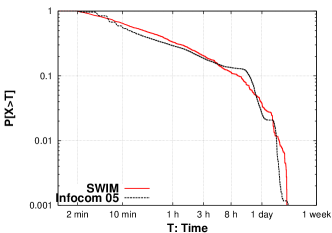
(a) Distribution of the inter-contact time in Infocom 05 and in SWIM

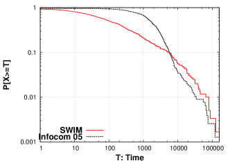
(b) Distribution of the contact duration for each pair of nodes in Infocom 05 and in SWIM

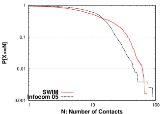
(c) Distribution of the number of contacts for each pair of nodes in Infocom 05 and in SWIM

Figure 1: SWIM and Infocom 05

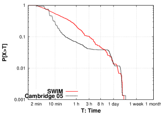
(a) Distribution of the inter-contact time in Cambridge 05 and in SWIM

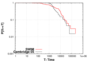
(b) Distribution of the contact duration for each pair of nodes in Cambridge 05 and in SWIM

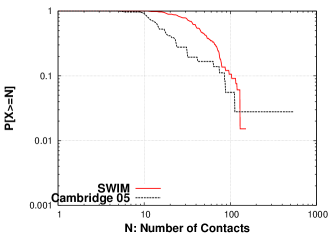
(c) Distribution of the number of contacts for each pair of nodes in Cambridge 05 and in SWIM

Figure 2: SWIM and Cambridge 05

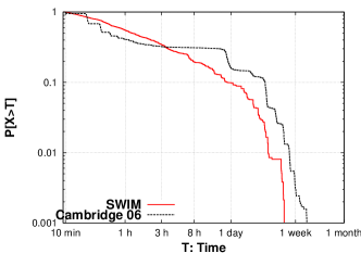
(a) Distribution of the inter-contact time in Cambridge 06 and in SWIM

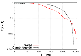
(b) Distribution of the contact duration for each pair of nodes in Cambridge 06 and in SWIM

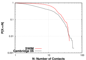
(c) Distribution of the number of contacts for each pair of nodes in Cambridge 06 and in SWIM

Figure 3: SWIM and Cambridge 06

The idea is to tune the few parameters used by SWIM in order to simulate Infocom 05, Cambridge 05, and Cambridge 06. For each of the experiments we consider the following metrics: inter-contact time CCD function, contact distribution per pair of nodes, and number of contacts per pair of nodes. The inter-contact time distribution is important in mobile networking since it characterizes the frequency with which information can be transferred between people in real life. It has been widely studied for real traces in a large number of previous papers [4, 5, 16, 8, 6, 12, 20]. The contact distribution per pair of nodes and the number of contacts per pair of nodes are also important. Indeed they represent a way to measure relationship between people. As it was also discussed in [21, 22, 23] it’s natural to think that if a couple of people spend more time together and meet each other frequently they are familiar to each other. Familiarity is important in detecting communities, which may help improve significantly the design and performance of forwarding protocols in mobile environments such as DNTs [23]. Let’s now present the experimental results obtained with SWIM when simulating each of the real scenarios of data sets. Since the scenarios we consider use iMotes, we model our network node according to iMotes properties (outdoor range $30\textrm{m}$). We initially distribute the nodes over a network area of size $300\times 300~{}\textrm{m}^{2}$. In the following, we assume for the sake of simplicity that the network area is a square of side 1, and that the node transmission range is 0.1. In all the three experiments we use a power law with slope $a=1.45$ in order to generate waiting time values of nodes when arriving to destination, with an upper bound of 4 hours. We use as $\textit{seen}(C)$ function the fraction of the nodes seen in cell $C$, and as $\textit{distance}(x,C)$ the following

$$\textit{distance}(x,C)=\frac{1}{\left(1+k||x-y||\right)^{2}},$$

where $x$ is the position of the home of the current node, and $y$ is the position of the center of cell $C$. Positions are coordinates in the square of size 1. Constant $k$ is a scaling factor, set to $0.05$, which accounts for the small size of the experiment area. Note that function $\textit{distance}(x,C)$ decays as a power law. We come up with this choice after a large set of experiments, and the choice is heavily influenced by scaling factors.

We start with Infocom 05. The number of nodes $n$ and the simulation time are the same as in the real data set, hence 41 and 3 days respectively. Since the area of the real experiment was quite small (a large hotel), we deem that $300\times 300~{}m^{2}$ can be a good approximation of the real scenario. In Infocom 05, there were many parallel sessions. Typically, in such a case one chooses to follow what is more interesting to him. Hence, people with the same interests are more likely to meet each other. In this experiment, the parameter $\alpha$ such that the output fit best the real traces is $\alpha=0.75$. The results of this experiment are shown in Figure 1.

We continue with the Cambridge scenario. The number of nodes and the simulation time are the same as in the real data set, hence 11 and 5 days respectively. In the Cambridge data set, the iMotes were distributed to two groups of students, mainly undergrad year 1 and  2, and also to some PhD and Master students. Obviously, students of the same year are more likely to see each other more often. In this case, the parameter $\alpha$ which best fits the real traces is $\alpha=0.95$. This choice proves to be fine for both Cambridge 05 and Cambridge 06. The results of this experiment are shown in Figure 2 and 3.

In all of the three experiments, SWIM proves to be an excellent way to generate synthetic traces that approximate real traces. It is particularly interesting that the same choice of parameters gets goods results for all the metrics under consideration at the same time.

VI Comparative performance of forwarding protocols

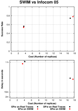
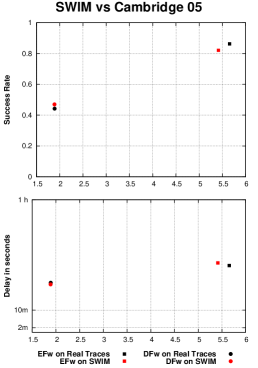
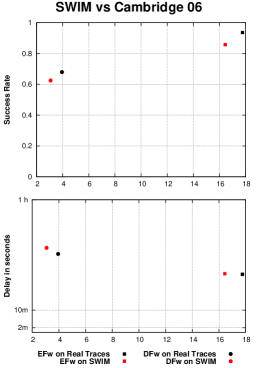
Figure 4: Performance of both forwarding protocols on real traces and SWIM traces. EFw denotes Epidemic Forwarding while DFwd Delegation Forwarding.

In this section we show other experimental results of SWIM, related to evaluation of two simple forwarding protocols for DNTs such as Epidemic Forwarding [9] and simplified version of Delegation Forwarding[10] in which each node has a random constant as its quality. Of course, this simplified version of delegation forwarding is not very interesting and surely non particularly efficient. However, we use it just as a worst case benchmark against epidemic forwarding, with the understanding that our goal is just to validate the quality of SWIM, and not the quality of the forwarding protocol.

In the following experiments, we use for each experiment the same tuning used in the previous section. That is, the parameters input to SWIM are not “optimized” for each of the forwarding protocols, they are just the same that has been used to fit real traces with synthetic traces.

For the evaluation of the two forwarding protocols we use the same assumptions and the same way of generating traffic to be routed as in [10]. For each trace and forwarding protocol a set of messages is generated with sources and destinations chosen uniformly at random, and generation times form a Poisson process averaging one message per 4 seconds. The nodes are assumed to have infinite buffers and carry all message replicas they receive until the end of the simulation. The metrics we are concerned with are: cost, which is the number of replicas per generated message; success rate which is the fraction of generated messages for which at least one replica is delivered; average delay which is the average duration per delivered message from its generation time to the first arrival of one of its replicas. As in [10] we isolated 3-hour periods for each data trace (real and synthetic) for our study. Each simulation runs therefore 3 hours. to avoid end-effects no messages were generated in the last hour of each trace.

In the two forwarding protocols, upon contact with node $A$, node $B$ decides which message from its message queue to forward in the following way:

• Epidemic Forwarding: Node $A$ forwards message $m$ to node $B$ unless $B$ already has a replica of $m$. This protocol achieves the best possible performance, so it yields upper bounds on success rate and average delay. However, it does also have a high cost.

• (Simplified) Delegation Forwarding: To each node is initially given a quality, distributed uniformly in $(0;1]$. To each message is given a rate, which, in every instant corresponds to the quality of the node with the best quality that message have seen so far. When generated the message inherits the rate from the node that generates it (that would be the sender for that message). Node $A$ forwards message $m$ to node $B$ if the quality of node $B$ is greater than the rate of the copy of $m$ that $A$ holds. If $m$ is forwarded to $B$, both nodes $A$ and $B$ update the rate of their copy of $m$ to the quality of $B$.

Figure 4 shows how the two forwarding protocols perform in both real and synthetic traces, generated with SWIM. As you can see, the results are excellent—SWIM predicts very accurately the performance of both protocols. Most importantly, this is not due to a customized tuning that has been optimized for these forwarding protocols, it is just the same output that SWIM has generated with the tuning of the previous section. This can be important methodologically: To tune SWIM on a particular scenario, you can concentrate on a few well known and important statistical properties like inter-contact time, number of contacts, and duration of contacts. Then, you can have a good confidence that the model is properly tuned and usable to get meaningful estimation of the performance of a forwarding protocol.

VII Conclusions

In this paper we present SWIM, a new mobility model for ad hoc networking. SWIM is simple, proves to generate traces that look real, and provides an accurate estimation of forwarding protocols in real mobile networks. SWIM can be used to improve our understanding of human mobility, and it can support theoretical work and it can be very useful to evaluate the performance of networking protocols in scenarios that scales up to very large mobile systems, for which we don’t have real traces.

References

- [1] T. Camp, J. Boleng, and V. Davies, “A survey of mobility models for ad hoc network research,” Wireless Communications and Mobile Computing Special issue on Mobile Ad Hoc Networking: Research, Trends and Applications, vol. 2, no. 5, pp. 483–502, 2002.
- [2] D. B. Johnson and D. A. Maltz, “Dynamic source routing in ad hoc wireless networks,” in Mobile Computing (Imielinski and Korth, eds.), vol. 353, Kluwer Academic Publishers, 1996.
- [3] J. Su, A. Chin, A. Popivanova, A. Goel, and E. de Lara, “User mobility for opportunistic ad-hoc networking,” in WMCSA ’04: Proceedings of the Sixth IEEE Workshop on Mobile Computing Systems and Applications, (Washington, DC, USA), pp. 41–50, IEEE Computer Society, 2004.
- [4] P. Hui, A. Chaintreau, J. Scott, R. Gass, J. Crowcroft, and C. Diot, “Pocket switched networks and human mobility in conference environments,” in WDTN ’05: Proceeding of the 2005 ACM SIGCOMM workshop on Delay-tolerant networking, pp. 244–251, ACM Press, 2005.
- [5] A. Chaintreau, P. Hui, J. Crowcroft, C. Diot, R. Gass, and J. Scott, “Impact of human mobility on the design of opportunistic forwarding algorithms,” in INFOCOM 2006. 25th IEEE International Conference on Computer Communications. Proceedings, 2006.
- [6] T. Karagiannis, J.-Y. L. Boudec, and M. Vojnović, “Power law and exponential decay of inter contact times between mobile devices,” in MobiCom ’07: Proceedings of the 13th annual ACM international conference on Mobile computing and networking, pp. 183–194, ACM, 2007.
- [7] A. Chaintreau, P. Hui, J. Crowcroft, C. Diot, R. Gass, and J. Scott, “Pocket switched networks: Real-world mobility and its consequences for opportunistic forwarding,” tech. rep., Computer Laboratory, University of Cambridge, 2006.
- [8] H. Cai and D. Y. Eun, “Crossing over the bounded domain: from exponential to power-law inter-meeting time in manet,” in MobiCom ’07: Proceedings of the 13th annual ACM international conference on Mobile computing and networking, pp. 159–170, ACM, 2007.
- [9] A. Vahdat and D. Becker, “Epidemic routing for partially connected ad hoc networks,” Tech. Rep. CS-200006, Duke University, 2000.
- [10] V. Erramilli, M. Crovella, A. Chaintreau, and C. Diot, “Delegation forwarding,” in MobiHoc ’08: Proceedings of the 9th ACM international symposium on Mobile ad hoc networking and computing, pp. 251–260, ACM, 2008.
- [11] I. Rhee, M. Shin, S. Hong, K. Lee, and S. Chong, “On the levy-walk nature of human mobility,” in INFOCOM 2008. IEEE International Conference on Computer Communications. Proceedings, 2008.
- [12] M. Musolesi and C. Mascolo, “Designing mobility models based on social network theory,” SIGMOBILE Mob. Comput. Commun. Rev., vol. 11, no. 3, pp. 59–70, 2007.
- [13] M. Piorkowski, N. Sarafijanovic-Djukic, and M. Grossglauser, “On Clustering Phenomenon in Mobile Partitioned Networks,” in The First ACM SIGMOBILE International Workshop on Mobility Models for Networking Research, ACM, 2008.
- [14] F. Ekman, A. Keränen, J. Karvo, and J. Ott, “Working day movement model,” in The First ACM SIGMOBILE International Workshop on Mobility Models for Networking Research, ACM, 2008.
- [15] M. C. Gonzalez, C. A. Hidalgo, and A.-L. Barabasi, “Understanding individual human mobility patterns,” Nature, vol. 453, pp. 779–782, june 2008.
- [16] J. Leguay, A. Lindgren, J. Scott, T. Friedman, and J. Crowcroft, “Opportunistic content distribution in an urban setting,” in CHANTS ’06: Proceedings of the 2006 SIGCOMM workshop on Challenged networks, pp. 205–212, ACM, 2006.
- [17] J. Scott, R. Gass, J. Crowcroft, P. Hui, C. Diot, and A. Chaintreau, “CRAWDAD trace cambridge/haggle/imote/cambridge (v. 2006–01–31).” Downloaded from http://crawdad.cs.dartmouth.edu/cambridge/haggle/imote/cambridge, jan 2006.
- [18] J. Leguay, A. Lindgren, J. Scott, T. Riedman, J. Crowcroft, and P. Hui, “CRAWDAD trace upmc/content/imote/cambridge (v. 2006–11–17).” Downloaded from http://crawdad.cs.dartmouth.edu/upmc/content/imote/cambridge, nov 2006.
- [19] J. Scott, R. Gass, J. Crowcroft, P. Hui, C. Diot, and A. Chaintreau, “CRAWDAD trace cambridge/haggle/imote/infocom (v. 2006–01–31).” Downloaded from http://crawdad.cs.dartmouth.edu/cambridge/haggle/imote/infocom, jan 2006.
- [20] H. Cai and D. Y. Eun, “Toward stochastic anatomy of inter-meeting time distribution under general mobility models,” in MobiHoc ’08: Proceedings of the 9th ACM international symposium on Mobile ad hoc networking and computing, pp. 273–282, ACM, 2008.
- [21] P. Hui, E. Yoneki, S. Y. Chan, J. Crowcroft, and J. Crowcroft, “Distributed community detection in delay tolerant networks,” in MobiArch ’07: Proceedings of first ACM/IEEE international workshop on Mobility in the evolving internet architecture, pp. 1–8, ACM, 2007.
- [22] E. Yoneki, P. Hui, S. Chan, and J. Crowcroft, “A socio-aware overlay for publish/subscribe communication in delay tolerant networks,” in MSWiM ’07: Proceedings of the 10th ACM Symposium on Modeling, analysis, and simulation of wireless and mobile systems, pp. 225–234, ACM, 2007.
- [23] P. Hui, J. Crowcroft, and E. Yoneki, “Bubble rap: social-based forwarding in delay tolerant networks,” in MobiHoc ’08: Proceedings of the 9th ACM international symposium on Mobile ad hoc networking and computing, pp. 241–250, ACM, 2008.