On the mean density of complex eigenvalues for an ensemble of random matrices with prescribed singular values

Abstract

Given any fixed $N\times N$ positive semi-definite diagonal matrix $G\geq 0$ we derive the explicit formula for the density of complex eigenvalues for random matrices $A$ of the form $A=U\sqrt{G}$

where the random unitary matrices $U$ are distributed on the group $\mathrm{U(N)}$ according to the Haar measure.

1 Introduction

The question of characterizing the locus of complex eigenvalues for an $N\times N$ matrix $A$ with prescribed singular values, that is eigenvalues $g_{i}\geq 0,\,\,i=1,\ldots,N$ of $A^{*}A$, , with $A^{*}$ being Hermitian conjugate of $A$, was considered in classical papers by Horn and Weyl [1]. In the present paper we provide a kind of statistical answer to that question. Define $G=\textrm{diag}(g_{1},\ldots,g_{N})\geq 0$, multiply the matrix $\sqrt{G}$ by a general unitary transformation $U$ from the left and average over the unitary group $\mathrm{U}(N)$ with the invariant (Haar) measure. This construction induces a natural measure on the set of matrices $A=U\sqrt{G}$ with given singular values $g_{i}$ and in this way provides us with the corresponding random matrix ensemble. The complex eigenvalues $z_{i}$ of such matrices $A$ will cover generically an annular domain $R_{min}<|z|<R_{max}$ in the complex plane with some density $\rho(z)$. In such an approach the statistical characterization of the locus of complex eigenvalues amounts to knowing the profile of the ensemble averaged value of that density for a given set of singular values. It is easy to understand that such mean density can depend only on $|z|$. The corresponding explicit formula is provided in Theorem 2.1 which is the main result of the paper.

Apart from being a rather nontrivial mathematical problem, understanding the statistical properties of complex eigenvalues of the above-mentioned ensemble is motivated by its applications in the domain of Quantum Chaotic Scattering. In this capacity the problem attracted attention for some time, and a few partial results were obtained previously in several limiting cases[2, 3, 4, 5, 6]. Below we give a brief description of the physical context related to the problem.

One of very useful instruments in the analysis of classical Hamiltonian systems with chaotic dynamics are the so-called area-preserving chaotic maps, see e.g. [7] and references therein. They appear naturally either as a mapping of the Poincaré section onto itself, or as a result of a ”stroboscopic” description of Hamiltonians which are periodic functions of time. Their quantum mechanical analogues are unitary operators which act on Hilbert spaces of finite large dimension $N$, and are often referred to as evolution, scattering or Floquet operators, depending on the given physical context. Their eigenvalues consist of $N$ points on the unit circle (eigenphases). Numerical studies of various classically chaotic systems suggest that the eigenphases conform statistically quite accurately the results obtained for unitary random matrices of a particular symmetry (Dyson circular ensembles).

Let us now imagine that a system represented by a chaotic map (”inner world”) is embedded in a larger physical system (”outer world”) in such a way that it describes particles which can come inside the region of chaotic motion and leave it after some time via $M$ open channels. Models of such type appeared in various disguises for example, in [8, 9, 10, 11] and most recently discussed in much detail in relation to properties of dielectric microresonators in [12]. A natural mathematical framework allowing to deal efficiently with such a situation was suggested in [4], see also [5] and we mention here only its gross features. For a closed quantum system characterized by a wavefunction $\Psi$ the ”stroboscopic” (discrete-time) dynamics amounts to a linear unitary map $\Psi(n)\to\Psi(n+1)$, such that $\Psi(n+1)=\hat{u}\Psi(n)$. The unitary evolution operator $\hat{u}$ describes the ”closed” inner state domain decoupled both from input and output spaces. Then a coupling that makes the system open must convert the evolution operator $u$ to a contractive operator $\hat{A}$ such that ${\bf 1}-\hat{A}^{*}\hat{A}\geq 0$. It is easy to show that one can always choose $\hat{A}=\hat{u}\sqrt{{\bf 1}-\hat{\tau}\hat{\tau}^{*}}$ where the matrix $\hat{\tau}$ is a rectangular $N\times M,M\leq N$ diagonal with the entries $\tau_{ij}=\delta_{ij}\tau_{j}\,,\,1\leq i\leq N\,,\,{1\leq j\leq M},\quad 0\leq\ \tau_{j}\leq 1$. With $\hat{u}$ replaced by $\hat{A}$, the equation $\Psi(n+1)=\hat{A}\Psi(n)$ then describes an irreversible decay of any initially prepared state $\Psi(0)\neq 0$, assuming that external input is absent during the subsequent evolution. The complex eigenvalues $z_{k}$ of the operator $\hat{A}$ all belong to the interior of the unit circle $|z|<1$ and play the role of resonances for the discrete time systems. Let us mention that various aspects of resonances associated with quantum chaotic open maps recently attracted considerable attention[12, 13].

The relation with the random matrix construction employed in this paper is now obvious. It amounts to replacing the true evolution operator $\hat{u}$ with its random matrix analogue $u$ taken from the Circular Unitary Ensemble (CUE) in accordance with the standard ideas of Quantum Chaos, and to denoting $G=\sqrt{{\bf 1}-\hat{\tau}\hat{\tau}^{*}}$. In this way the task of studying resonances is reduced to investigating eigenvalues of random matrices $A$ of the specified type.

The first significant random matrix result on such matrices $A$ seems to have appeared in [2] where the authors considered so-called ”truncations” of random unitary matrices. In our notations that case is equivalent to taking $g_{1}=g_{2}=\ldots g_{M}=0$, with all the rest $N-M$ of $g_{i}$ being equal to unity. In [4] the mean density of complex eigenvalues was derived in the limit $N\to\infty$, with $M<\infty$ being fixed and all $g_{i}\leq 1$. The work [5] provided some general results on the joint probability density of all $N$ complex eigenvalues $z_{i}$, as well as a few formulae for the few-point correlation functions (the so-called marginal distributions) of the eigenvalue densities. Those formulae however only lead to explicit managable expressions again in the same limiting case as in [4]. As to the results valid for arbitrary finite $N$, only the simplest particular case $g_{1}=g_{2}=\ldots=g_{N-1}=g,\,g_{N}<g$ was so far addressed by a variety of methods, see [6] for the most recent account and [3] for an early consideration.

2 Statement of the Main Results

Our results show that the ensemble-averaged eigenvalue density function $\rho(z)=\Psi(|z|^{2})$, i.e. indeed depends only on $|z|$. To write the function $\Psi$ explicitly we need to introduce a few notations.

Let $\mathrm{s}^{l}$ be the $l$-th order elementary symmetric polynomials of $g_{i},\ i=1,\dots,N$, e.g. $\mathrm{s}^{0}=1,\ \mathrm{s}^{1}=\sum_{i=1}^{N}g_{i},\ \mathrm{s}^{2}=\sum_{i<j}^{N}g_{i}g_{j},\ \dots$, etc. Let us denote $\mathrm{s}^{l}_{[i_{1},i_{2},\dots]}=\mathrm{s}^{l}|_{g_{i_{1}}=g_{i_{2}}=\dots=0}$. Define the following functions of $\{g_{i}\}$ and the complex variable $z$:

$$\mathrm{F}_{-}(g_{i}) =-\frac{1}{{{\prod^{\prime}}_{j=1}^{N}}(g_{i}-g_{j})}Ng_{i}^{N-1}\sum\limits_{l=0}^{N-1}\mathrm{s}^{l}_{[i]}|z|^{2(-l-1)}\,\frac{l}{\left(\!\!\!\begin{array}[]{c}N\!-\!1\\ l\end{array}\!\!\!\right)}$$ (2.3)

$$\mathrm{F}_{+}(g_{i}) =\mathrm{F}_{-}(g_{i})+\mathrm{F}_{\Delta}(g_{i})$$ (2.4)

$$\mathrm{F}_{\Delta}(g_{i}) =\frac{1}{{\prod\limits_{j=1}^{N}}^{\prime}(g_{i}-g_{j})}(g_{i}-|z|^{2})^{N-2}\sum\limits_{l=0}^{N-1}\mathrm{s}^{l}_{[i]}|z|^{-2(l+1)}\frac{1}{\left(\!\!\!\begin{array}[]{c}N\!-\!1\\ l\end{array}\!\!\!\right)}\bigg{[}lg_{i}+(N-1-l)|z|^{2}\bigg{]}$$ (2.7)

$$=\frac{(g_{i}-|z|^{2})^{N-2}}{{\prod\limits_{j=1}^{N}}^{\prime}(g_{i}-g_{j})}\int_{0}^{\infty}\frac{Ndt}{(1+t)^{N+2}}\det\bigg{(}1+\frac{t}{|z|^{2}}G_{[i]}\bigg{)}\bigg{[}N-t+\frac{g_{i}}{|z|^{2}}(Nt-1)\bigg{]}\;,$$ (2.8)

where we used the binomial function $\left(\!\!\begin{array}[]{c}N\\ l\end{array}\!\!\right)=\frac{N!}{l!(N-l)!}$. In Eq.(2.7), we defined a matrix $G_{[i]}=\textrm{diag}(g_{1},\dots,g_{i-1},g_{i+1},\dots,g_{N})$ and used the dash to denote that the index $j$ can not be equal to $i$ in the product.

The main statement of the paper is that the density of complex eigenvalues can be written in terms of the functions defined above. More precisely, we state the following

Theorem 2.1 Let $U\in\mathrm{U}(N)$ be an element of the unitary group and $G=\textrm{diag}(g_{1},\dots,g_{N})$ be a fixed positive diagonal matrix, such that $0<g_{1}<\dots<g_{N}<\infty$. Let $U$ be distributed on $\mathrm{U}(N)$ according to the Haar measure. Then the mean density $\rho(z)$ of complex eigenvalues of the matrix $A=U\sqrt{G}$ is given by

$$\rho(z)=\Psi(|z|^{2})=\frac{1}{N}\sum_{i=1}^{N}\mathrm{F}_{\sigma}(g_{i})\;,$$ (2.9)

where $\sigma=+$ for $|z|^{2}>g_{i}$, $\sigma=-$ for $|z|^{2}<g_{i}$.

Remark: Exploiting that the function $\mathrm{F}_{-}$ is totally antisymmetric with respect to all $g_{i}$’s, we can rewrite the above expression in the form:

$$\Psi(|z|^{2})=\left\{\begin{array}[]{ll}0&|z|^{2}<g_{1}<g_{2}\dots<g_{N}\\ \!\!\frac{1}{N}\sum\limits_{i=k+1}^{N}\mathrm{F}_{\Delta}(g_{i})&g_{1}<\dots<g_{k}<|z|^{2}<g_{k+1}<\dots<g_{N}\\ 0&g_{1}<g_{2}\dots<g_{N}<|z|^{2}\end{array}\right.$$ (2.13)

Remark: For $N>3$, it is not difficult to show that the eigenvalue density function is ’smooth’ at each $|z|=g_{i},1<i<N$, that is it has a continuous derivative. When $N=3$, the density function is only ’continuous’ at $g_{2}$ but not ’smooth’.

In the case of degenerate eigenvalues of the matrix $G$ the density function can be derived from Theorem 2.1 by taking the corresponding limits as shown below.

Corollary 2.2: Suppose the diagonal matrix $G$ has the following degeneracies,

$$g_{k_{1}}=\dots=g_{k_{1}+i_{1}},\ \ g_{k_{2}}=\dots=g_{k_{2}+i_{2}},\ \ \dots,\ \ g_{k_{s}}=\dots=g_{k_{s}+i_{s}}\;,$$ (2.14)

which is denoted by the short-hand notation

$${G}=\textrm{diag}(\dots,[g_{k_{1}},\dots,g_{k_{1}+i_{1}}],\dots,[g_{k_{s}},\dots,g_{k_{s}+i_{s}}],\dots)\;.$$ (2.15)

Define the following two functions

$$\mathrm{f}^{[k,i]}_{n}(g)\overset{\mbox{\tiny def}}{=}\frac{(g-|z|^{2})^{N-2}}{\prod\limits_{j=1}^{k-1}\prod\limits_{j=k+i+1}^{N}(g-g_{j})}\sum\limits_{l=n}^{N-1}\mathrm{s}^{l-n}_{[k,\dots,k+n]}|z|^{-2(l+1)}\frac{1}{\left(\begin{array}[]{c}\!\!\!N\!-\!1\\ l\end{array}\!\!\!\right)}\bigg{[}lg+(N-1-l)|z|^{2}\bigg{]}\;,$$ (2.18)

$$\mathrm{F}^{[k,i]}_{\Delta}\stackrel{{\scriptstyle\mbox{\tiny def}}}{{=}}\sum\limits_{n=0}^{i}\frac{(-)^{n}}{(i-n)!}\frac{d^{i-n}}{dg^{i-n}_{k+n}}\mathrm{f}^{[k,i]}_{n}(g_{k+n})\;.$$ (2.19)

The density function is then given by replacing each $\sum_{n=0}^{i}\mathrm{F}_{\Delta}(g_{k+n})$ in the Theorem by $\mathrm{F}_{\Delta}^{[k,i]}$ and making substitutions Eq.(2.14).

Proof: Consider the following sum: $\psi=\sum_{n=0}^{i}\mathrm{F}_{\Delta}(g_{k+n})$ when $g_{k}=\dots=g_{k+i}$. Taking the limit $g_{k+i-1}\to g_{k+i}=g$ yields

$$\lim_{g_{k+i-1}\to g_{k+i}=g}\psi$$

$$= \left(\sum\limits_{n=0}^{i-2}\mathrm{F}_{\Delta}(g_{k+n})+\frac{d}{dg_{k+i-1}}(g_{k+i-1}-g_{k+i})(\mathrm{F}_{\Delta}(g_{k+i-1})+\mathrm{F}_{\Delta}(g_{k+i}))\right)_{g_{k+i-1}=g_{k+i}=g}$$

$$= \left(\sum\limits_{n=0}^{i-2}\mathrm{F}_{\Delta}(g_{k+n})+\frac{d}{dg_{k+i-1}}\left[\mathrm{f}_{0}^{[k+i-1,1]}(g_{k+i-1})-\mathrm{f}_{1}^{[K+i-1,1]}(g_{k+i})\right]\right)_{g_{k+i-1}=g_{k+i}=g}$$

$$= \ \mathrm{F}_{\Delta}^{[k+i-1,1]}|_{g_{k+i-1}=g_{k+i}=g}\;.$$ (2.20)

In the second step we have exploited the linearity of $\mathrm{s}^{l}$ as a function of $g$’s. Next, we take the limit $g_{k+i-2}\to g$. Repeating the procedure $i$ times, we arrive at

$$\psi|_{g_{k}=\dots=g_{k+i}=g}=\mathrm{F}_{\Delta}^{[k,i]}|_{g_{k}=\dots=g_{k+i}=g}\;.$$ (2.21)

Applying the results Eq.(2.21) to other degeneracies, we obtain the eigenvalue density function for $U\sqrt{G}$ under the condition Eq.(2.14).          $\Box$

Example 1(rank-one deviation from unitary matrix):
In the special case of $G=\textrm{diag}(g_{1},[g_{2},\dots,g_{N}])$, with $g_{2}=\dots=g_{N}=g$, the above procedure leads to an especially simple formula for the mean eigenvalue density:

$$\Psi=\frac{(|z|^{2}-g_{1})^{N-2}}{(g-g_{1})^{N-1}|z|^{2N}}\!\left((N-1)(|z|^{2N}+g^{N-1}g_{1})+\!\!\sum\limits_{k=0}^{N-2}\left[(N-2-k)g+kg_{1}\right]g^{k}|z|^{2(N-1-k)}\right)\;.$$ (2.22)

which coincides with the known result [3, 6].

Remark: In Eq.(2.22), as $g\to g_{1}$, the density function $\Psi\to\infty$ on $[g_{1},g]$ and is zero otherwise. On the other hand, the integration of $\Psi$ over the region $[g_{1},g]$ yields one. We conclude that in this case the density function is simply $\delta(g-|z|^{2})$, as it must be for a random matrix $A=U\sqrt{g}$ which is simply proportional to CUE matrix.

Remark: In fact, in our derivation of the main theorem, we can extend the domain of $g_{i}$’s to include the origin, i.e. our formula holds for $g_{i}\geq 0$. We illustrate this observation in the following example.

Example 2(truncated unitary matrix):
Consider the case $G=\textrm{diag}([g_{1},\dots,g_{M}],[g_{M+1},\dots,g_{N}])$, where $g_{1}=\dots=g_{M}=0$ and $g_{M+1}=\dots=g_{N}=1$. By Corollary, we can write the density function of eigenvalues of $A=U\sqrt{G}$ as

$$\Psi= \ \mathrm{F}^{[M+1,N-M-1]}_{\Delta}|_{g_{1}=\dots=g_{M}=0,g_{M+1}=\dots=g_{N}=1}$$

$$\propto \ (1-|z|^{2})^{M-1}\left(\frac{d}{d|z|^{2}}\right)^{M}\frac{1-|z|^{2N}}{1-|z|^{2}}\;.$$ (2.23)

In the first step, we have extended domains of $g$ to $[0,\infty)$ in Theorem 2.1, and correspondingly, Corollary 2.2. In fact, when $G=\textrm{diag}(0\cdot I_{M},I_{N-M})$, eigenvalues of the matrix $A$ in Example 2. coincide with those of $(N-M)\times(N-M)$ lower right sub-block of a random unitary matrix, also known as the ’truncated’ unitary matrix. Same results as Eq.(2) has been obtained with a completely different method in [2].

Remark: As we can obviously always absorb the $\mathrm{U}^{N}(1)$ phase of $N\times N$ complex diagonal matrix into $U$, the domain for the matrix $G$ can be defined on $\mathbb{C}_{1}^{N}$. The eigenvalue density function of $U\sqrt{G}$, averaged over CUE is then obtained by substituting $g_{i}\to|g_{i}|$ into Theorem 2.1.

Finally, we compare our formula Eq.(2.13) with numerical simulations. To this end, we choose a fixed diagonal matrix $G$ and generate unitary matrices according to the Haar measure. We draw a histogram of the radial part of eigenvalues, $|z|$, of the matrix $U\sqrt{G}$, see Fig.1 To compare with the histogram, we define the appropriately modified density function $\Psi_{1}(|z|)=2|z|\Psi(|z|^{2})$, which is shown by the solid line. From Fig. 1, we observe a very good match between our formula Eq.(2.13) and the results of numerical simulations.

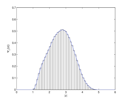
Figure 1: Histogram of the radial part of the eigenvalue distribution of $5\times 5$ matrices $A=U\sqrt{G}$. Here $G=\textrm{diag}(1,4,9,16,25)$ and $U$ is the Haar-distributed unitary matrix, with sample size 100000 and bin 0.10. Solid line represents the function $\Psi_{1}(|z|)$ as derived from Eq.(2.13).

3 Main steps of the proof

3.1 Colour-flavour transformation

Our starting expression is the following formula [14, 15] for the averaged density of complex eigenvalues for a general finite-size non-Hermitian random matrix $A$

$$\rho(z)=-\frac{1}{\pi}\lim_{\kappa\to 0}\frac{\partial}{\partial{\bar{z}}}\lim_{z_{b}\to z}\frac{\partial}{\partial{z_{b}}}\Bigg{<}\frac{\det\left(\begin{array}[]{cc}\kappa&i(z-A)\\ i(\bar{z}-A^{\dagger})&\kappa\end{array}\right)}{\det\left(\begin{array}[]{cc}\kappa&i(z_{b}-A)\\ i(\bar{z}_{b}-A^{\dagger})&\kappa\end{array}\right)}\Bigg{>}_{U}\;.$$ (3.28)

In our case $A=U\sqrt{G}$, where $U\in\mathrm{U}(N)$, $G=\textrm{diag}(g_{1},\dots,g_{N})>0$. Averaging over the Haar measure on the unitary group $\mathrm{U}(N)$ is denoted by $<\cdots>_{U}$.

Introduce vectors $S_{a}=(s_{a}^{i})$ with complex components and their counterparts $\chi_{a}=(\chi_{a}^{i})$ with anti-commuting components (Grassmann variables), for all $i=1,\dots,N$ and $a=1,2$. This defines two sets of (graded) vectors $\psi^{i}_{a}=\left(\begin{array}[]{c}s^{i}_{a}\\ \chi^{i}_{a}\end{array}\right)$ with $a=1,2$. The determinants can be represented as integrals over complex variables $s$ and Grassmann variables $\chi$ in the standard way:

$$<\cdots>_{U}\propto \int dU\int dS_{1}dS_{2}\exp\left[-\kappa(S_{1}^{\dagger}S_{1}+S_{2}^{\dagger}S_{2})-i(z_{b}S^{\dagger}_{1}S_{2}+\bar{z}_{b}S^{\dagger}_{2}S_{1})\right]$$

$$\int d\chi_{1}d\bar{\chi}_{1}d\chi_{2}d\bar{\chi}_{2}\ \exp\left[-\kappa(\chi_{1}^{\dagger}\chi_{1}+\chi_{2}^{\dagger}\chi_{2})-i(z\chi^{\dagger}_{1}\chi_{2}+\bar{z}\chi^{\dagger}_{2}\chi_{1})\right]$$

$$\ \exp i\left[\bar{\psi}_{1}^{i}A_{ij}\psi_{2}^{j}+\bar{\psi}_{2}^{i}A_{ij}^{\dagger}\psi_{1}^{j}\right]\;,$$ (3.29)

where we defined $dS_{1}\,dS_{2}=\prod_{a=1}^{2}\prod_{i=1}^{N}d\bar{s}_{a}^{i}ds_{a}^{i}$. Note that by Eq.(3.28), averaging over the unitary group in the above expression should be carried out after performing the integral over the graded vectors $\{\psi,\bar{\psi}\}$.

Next we change the order of integration over $\{\psi,\bar{\psi}\}$ and $\mathrm{U}(N)$, which is possible due to the fact that $\mathrm{U}(N)$ is compact and the integral is bounded. The integration over the unitary group can be performed explicitly by exploiting the colour-flavour transformation discovered by Zirnbauer [16]:

$$\int dU\exp\mathrm{i}\left[\bar{\psi}_{1}^{i}A_{ij}\psi_{2}^{j}+\bar{\psi}_{2}^{i}A_{ij}^{\dagger}\psi_{1}^{j}\right]=\int D(Q,\tilde{Q})\ \exp\mathrm{i}\left[\bar{\psi}_{1}^{i}Q\psi_{1}^{i}+g_{i}\bar{\psi}_{2}^{i}\tilde{Q}\psi_{2}^{i}\right]\;.$$ (3.30)

Such a transformation trades the integration over $\mathrm{U}(N)$, where N can be an arbitrary large integer for the integration over a considerably simpler $2\times 2$ graded matrices $Q$ defined as

$$Q=\left(\begin{array}[]{cc}q_{b}&\eta_{1}\\ \eta_{2}&q_{f}\end{array}\right),\hskip 14.22636pt\tilde{Q}=\left(\begin{array}[]{cc}\bar{q}_{b}&\sigma_{1}\\ \sigma_{2}&-\bar{q}_{f}\end{array}\right)\;.$$ (3.35)

Such $Q$ belongs to a Riemannian symmetric superspace [17] of the type $\mathrm{AIII|AIII}$. Here, $\eta$’s and $\sigma$’s are anti-commuting Grassmann variables. The so-called boson-boson and fermion-fermion blocks of $Q$ are given by

$$q_{b}\in\mathrm{U(1,1)/U(1)\times U(1)}=\mathrm{H}^{2}\ {\mathrm{and}}\ q_{f}\in\mathrm{U(2)/U(1)\times U(1)=S^{2}}\;.$$ (3.36)

The invariant measure on this domain is defined as

$$D(Q,\tilde{Q})=\mathrm{Sdet}^{N}(1-\tilde{Q}Q)dQd\tilde{Q}\;.$$ (3.37)

where $dQd\tilde{Q}=d^{2}q_{b}d^{2}q_{f}d\sigma_{1}d\sigma_{2}d\rho_{1}d\rho_{2}$.

After the colour-flavour transformation Eq.(3.30), we get

$$<\cdots>_{U}\ \propto F(\kappa)=\int d\bar{\psi}d\psi\int D(Q,\tilde{Q})\exp-(\bar{\psi}_{1}^{i},\bar{\psi}_{2}^{i})\left(\begin{array}[]{cc}\kappa-iQ&\mathrm{i}Z\\ &\\ \mathrm{i}\bar{Z}&\kappa-ig_{i}\tilde{Q}\end{array}\right)\left(\begin{array}[]{l}\psi_{1}^{i}\\ \psi_{2}^{i}\end{array}\right)\;,$$ (3.43)

where $d\bar{\psi}d\psi=dS_{1}^{2}dS_{2}^{2}d\chi_{1}d\bar{\chi}_{1}d\chi_{2}d\bar{\chi}_{2}$ and we defined

$$Z=\left(\begin{array}[]{cc}z_{b}&0\\ 0&z\end{array}\right)\ \ \mathrm{and}\ \ \bar{Z}=\left(\begin{array}[]{cc}\bar{z}_{b}&0\\ 0&\bar{z}\end{array}\right)\;.$$ (3.48)

For a fixed complex number $z$ and a given diagonal matrix $G$, the integral in Eq.(3.43), defines a function $F(\kappa)$ of the variable $\kappa$. Using the integral representation for Bessel functions we can show that $F(\kappa)$ is analytic in the half plane $\mathrm{Re}\ \kappa\!>\!0$.

3.2 Integration over $Q$ and analytic continuation

Direct evaluation of the integral over the graded matrix $Q$ followed by the integration over $\psi$ in Eq.(3.43) is very difficult. In fact, it is already a highly involved task in a much simpler case where $Q$ is a complex number and $\psi$ is a complex vector, see [6] for the corresponding calculation in such a case. A natural way out could be changing the order of integration in Eq.(3.43) in order to integrate first over $\{\psi,\bar{\psi}\}$ by using the standard Gaussian integral formula for graded vectors. However, extra care must be taken in performing such a change. To understand this consider the integral involving the boson-boson part of the supermatrix $Q$ and the complex vectors $S_{1}$ and $S_{2}$,

$$I_{\mathrm{bosonic}}=\int dS_{1}dS_{2}\int_{|q_{b}|\leq 1}dq_{b}^{2}\ \mathrm{e}^{-\kappa(S_{1}^{\dagger}S_{1}+S_{2}^{\dagger}S_{2})-(iz_{b}S_{1}^{\dagger}S_{2}+i\bar{z}_{b}S_{2}^{\dagger}S_{1})+iq_{b}S_{1}^{\dagger}S_{1}+i\bar{q}_{b}g_{i}\bar{S}_{2}^{i}S_{2}^{i}}\;,$$ (3.49)

where we have omitted the trivial Grassmann integrals. Changing the order of integration in Eq.(3.43) we arrive at

$$\tilde{I}_{\mathrm{bosonic}}=\int_{|q_{b}|\leq 1}dq_{b}^{2}\int dS_{1}dS_{2}\ \mathrm{e}^{-\kappa(S_{1}^{\dagger}S_{1}+S_{2}^{\dagger}S_{2})-(iz_{b}S_{1}^{\dagger}S_{2}+i\bar{z}_{b}S_{2}^{\dagger}S_{1})+iq_{b}S_{1}^{\dagger}S_{1}+i\bar{q}_{b}g_{i}\bar{S}_{2}^{i}S_{2}^{i}}\;.$$ (3.50)

It is clear that $\tilde{I}_{\mathrm{bosonic}}$ is only well-defined in $\mathrm{Re}\,\kappa\in(1,\infty)$. For $\kappa\to 0$, which is the limit we have to perform in the very end of the calculation, the integration over the boson-boson domain forbids changing integration order in Eq.(3.43). Actually, such a problem was first noticed in [6], and solved by modifying in a non-trivial way the domain of integration Eq.(3.36) over bosonic variables in the colour-flavour transformation. After such a modification one can actually carry out the required change of integration order for any $\kappa>0$. We shall however see that one can work in the standard parametrisation Eq.(3.36) in the allowed region $\mathrm{Re}\kappa\!\!>\!\!1$, and then continue to $0<\mathrm{Re}\,\kappa<1$ exploiting analytic properties of the function $F(\kappa)$.

Let us from now on work in the domain $\mathrm{Re}\ \kappa\!\!>\!\!1$. Substituting the transformation Eq.(3.30) into Eq.(3.1), changing the order of integrations over graded vectors $\{\psi,\bar{\psi}\}$ and the graded matrix $Q$ and integrating out $\{\psi,\bar{\psi}\}$, we get

$$G(\kappa)= \int dQd\tilde{Q}\ \mathrm{Sdet}^{N}(1-\tilde{Q}Q)\prod^{N}_{i=1}\mathrm{Sdet}^{-1}\left[\begin{array}[]{cc}\kappa-iQ&i\left(\begin{array}[]{cc}z_{b}&0\\ 0&z\end{array}\right)\\ &\\ i\left(\begin{array}[]{cc}\bar{z}_{b}&0\\ 0&\bar{z}\end{array}\right)&\kappa-ig_{i}\tilde{Q}\end{array}\right]\;.$$ (3.58)

Performing the integration over the supermatrix $Q$ is still a rather involved technical problem. We provide below a few comments related to it.

The Grassmann variables can be integrated out at any stage, and and we find it convenient to carry out that integration at the very beginning. On the other hand, it turns out to be important that the integration over the boson-boson part of $Q$ (i.e. $q_{b}$) should be performed before the fermion-fermion part $q_{f}$. In fact, a quick inspection of the $q_{f}$ integrals in Eq.(3.58) shows that they diverge logarithmically. However, those logarithmic divergences are actually a spurious feature of the colour-flavour transformation. The correct way of treating such divergencies when performing any supersymmetric colour-flavour transformation is to integrate first over the boson-boson sub-manifold. Then, combining all terms which are logarithmically divergent, one can show that the divergent parts cancel each other and the result is actually finite.

To perform the integration over the boson-boson part of $Q$, we introduce polar coordinates $q_{b}=\sqrt{r}e^{\mathrm{i}\theta}$, where $r\in[0,1],\theta\in[0,2\pi]$ so that $dq_{b}d\bar{q}_{b}=drd\theta$. In Eq.(3.58), $G(\kappa)$ is defined for $\mathrm{Re}\ \kappa\!\!>\!\!1$. For simplicity, we focus on the real $\kappa>1$. And further more, we assume all $g_{i}<1$, for $i=1,\dots,N$. This is done for convenience only and does not reduce generality as we can always scale the $G$-matrix by the magnitude of the largest eigenvalue, and at the end of the calculation to scale it back. Under these assumptions we can integrate over the angular variable $\theta$ by residue theorem. In this way the result of the original integration naturally splits into a sum of contributions from different residues.

It is crucial that after integrating over $\theta$, we can show $G(\kappa)$ is analytic in the half plane $\mathrm{Re}\ \kappa\!\!>\!\!0$. Therefore we are allowed to make the required analytic continuation on $G(\kappa)$ to $\mathrm{Re}\ \kappa\!\!>\!\!0$. Since both $F(\kappa)$ and $G(\kappa)$ are now analytic functions on $\mathrm{Re}\ \kappa\!\!>\!\!0$ and $F(\kappa)=G(\kappa)$ on $\kappa\!\!>\!\!1$, we conclude that $F(\kappa)=G(\kappa)$. We emphasis that this continuation is possible to carry out only after angular integration is performed under the assumption $\kappa\!>\!1$.

Knowing that we should take the limit $\kappa\to 0$ in the end of the calculation, we can use the condition $\kappa<<1$ to simplify significantly the integration over the radial part of $q_{b}$. It turns out that one has to distinguish two essentially different cases: $g_{i}>|z|^{2}$ and $g_{i}<|z|^{2}$. Each of these two cases yields different result when integrating over $q_{b}$ which explains why we have to distinguish $F_{+}(g_{i})$ from $F_{-}(g_{i})$ in the final expression. Integration over the fermion-fermion part of $Q$ uses certain properties of elementary symmetric functions but is otherwise straightforward. Finally, taking derivatives with respect to $z_{b}$ and $z$ and letting $\kappa\to 0$, we arrive after straightforward but still cumbersome calculations to the formula Eq.(2.9).

4 Open problems

In conclusion, we would like to mention a few open problems and possible extensions along the lines of the present work. An interesting problem would be to investigate the density of complex eigenvalues in the limit $N\to\infty$ assuming that the matrix $g$ has a finite limiting density $\nu(g)=\frac{1}{N}\sum_{i}\delta(g-g_{i})$ of eigenvalues $g_{i}$ in an interval of the $g-$axis. A special variant of the problem is to assume that $g_{i}$ are eigenvalues of some random Hermitian matrix with rotationally invariant measure. This case is in fact equivalent to the so-called Feinberg-Zee problem, see [18], which attracted a considerable interest recently. We hope to address it in our future publications.

Another important extension would be to replace matrices $U$ by unitary symmetric random matrices, or to take them from some other groups (e.g. orthogonal). The corresponding colour-flavour transformations are known, but the calculations seem to be extremely challenging technically.

References

• [1] Horn A, On the eigenvalues of a matrix with prescribed singular values, Proc. Am. Math. Soc 5 (1954) 4-7;
Weyl H, Inequalities between the two kinds of eigenvalues of a linear transformation, Proc.Nat.Acad.Sci. USA 35 (1949) 408-411.
• [2] Ε»yczkowski K and Sommers H-J, Truncations of random unitary matrices, J. Phys. A: Math. Gen. 33 (2000) 2045-2057.
• [3] Fyodorov YV, 2001 in Disordered and Complex Systems edited by P.Sollich et al. AIP Conference Proceedings 553 191 (Melville NY) [arXiv:nlin.CD/0002034].
• [4] Fyodorov YV and Sommers H-J, Spectra of random contractions and scattering theory for discrete-time systems, JETP Letters 72 (2000) 422-427.
• [5] Fyodorov YV and Sommers H-J, Random matrices close to Hermitian or unitary: overview of methods and results, J. Phys. A:Math.Gen. 36 (2003) 3303-3347.
• [6] Fyodorov YV, Khoruzhenko BA, On absolute moments of characteristic polynomials of a certain class of complex random matrices., Commun. Math. Phys. 273 (2007) 561-599.
• [7] Haake F. 1999 Quantum Signatures of Chaos (Springer, 2nd ed.).
• [8] GlΓΌck M, Kolovski AR and Korsch HJ, Wannier-Stark resonances in optical and semiconductor superlattices, Phys.Rep 366 (2002) 103-182.
• [9] Jacquod P, Schomerus H, and Beenakker CWJ, Quantum andreev map: A paradigm of quantum chaos in superconductivity, Phys.Rev.Lett. 90 (2003) 207004 (4p);
Tworzydlo J, et al., Dynamical model for the quantum-to-classical crossover of shot noise, Phys.Rev. B 68 (2003) 115313 (6pp);
Schomerus H and Jacquod P, Quantum-to-classical correspondence in open chaotic systems, J. Phys. A: Math.Gen. 38 (2005) 10663-10682.
• [10] Ossipov A, Kottos T, and Geisel T, Fingerprints of classical diffusion in open 2D mesoscopic systems in the metallic regime, Europh. Lett. 62 (2003) 719-725.
• [11] Prange RE , Resurgence in Quasiclassical Scattering, Phys.Rev.Lett. (2003) 90 070401 (4pp).
• [12] Keating JP, Novaes M, and Schomerus H, Model for chaotic dielectric microresonators, Phys.Rev. A 77 (2008) 013834 (9pp).
• [13] Nonnenmacher S, Zworski M, Fractal Weyl laws in discrete models of chaotic scattering, J. Phys. A: Math.Gen. 38 10683-10702 ; Nonnenmacher S, Rubin M, Resonant eigenstates for a quantized chaotic system, Nonlinearity 20 (2007) 1387-1420 ; Nonnenmacher S, Schenck E , Resonance distribution in open quantum chaotic systems, Preprint : arXiv:0803.1075.
• [14] Fyodorov YV, Khoruzhenko BA and Sommers H-J, Almost-Hermitian random matrices: eigenvalue density in the complex plane, Physics Letters 226 (1997) 46-52.
• [15] Fyodorov YV and Sommers H-J, Statistics of resonance poles, phase shifts and time delays in quantum chaotic scattering: random matrix approach for systems with broken time-reversal invariance J. Math. Phys. 38 (1997) 1918-1981.
• [16] Zirnbauer MR, Supersymmetry for systems with unitary disorder: circular ensembles, J. Phys. A: Math.Gen. 29 (1996) 7113-7136.
• [17] Zirnbauer MR, Riemannian symmetric superspaces and their origin in random-matrix theory, J. Math. Phys. 37 (1996) 4986-5018.
• [18] Feinberg J and Zee A, Non-Gaussian Non-Hermitean Random Matrix Theory: phase transitions and addition formalism, Nucl. Phys. B 501 (1997) 643-669; Feinberg J, Scalettar R. and Zee A, Single Ring Theorem and the Disk-Annulus Phase Transition, J Math Phys 42 (2001) 5718-5740.