Apply current exponential de Finetti theorem to realistic quantum key distribution

Abstract

In the realistic quantum key distribution (QKD), Alice and Bob respectively get a quantum state from an unknown channel, whose dimension may be unknown. However, while discussing the security, sometime we need to know exact dimension, since current exponential de Finetti theorem, crucial to the information-theoretical security proof, is deeply related with the dimension and can only be applied to finite dimensional case. Here we address this problem in detail. We show that if POVM elements corresponding to Alice and Bob’s measured results can be well described in a finite dimensional subspace with sufficiently small error, then dimensions of Alice and Bob’s states can be almost regarded as finite. Since the security is well defined by the smooth entropy, which is continuous with the density matrix, the small error of state actually means small change of security. Then the security of unknown-dimensional system can be solved. Finally we prove that for heterodyne detection continuous variable QKD and differential phase shift QKD, the collective attack is optimal under the infinite key size case.

I Introduction:

Information-theoretical security proof Renner thesis is a powerful and general way to prove the security for quantum key distribution (QKD). In this method, to give the amount of unconditional secret keys, we only need to discuss upper or lower bounds of some entropies. The exponential de Finetti theorem is crucial to this method, which support that as the key size goes to infinite, Eve cannot get more information from the coherent attack than from the collective attack Renner thesis . Since in the collective attack Eve attacks each signal independently with the same method, it is much easy for us to discuss the security. However, current exponential de Finetti theorem relying on the dimension and even diverges if the dimension is infinite, while in practice the dimension is often unknown or infinite.

There are also some other kind of quantum de Finetti theorems. In Ref. Matthias ; Matthias2 ; finite de fi , several de Finetti theorems for different conditions are given. These de Finetti theorems can be independent with the dimension. Even under the infinite dimensional case, they still converge. However, These de Finetti theorems are polynomial and not exponential. As the key size goes to infinite, they can not exponentially converge to zero. Whether such polynomial de Finetti theorems can be applied to QKD requires further discussion.

We can think about a more general case. Alice and Bob respectively get a quantum state from a channel and do measurement and thus hold classical data finally. Realistically, they only know the classical data and do not know anything about the dimension of quantum state beforehand. Therefore, it is not realistic for us to assume the dimension before discussing the security. If the dimension of quantum state is unknown, current exponential de Finetti theorem may not be directly applied and the security against the most general attack is difficult to given by the information-theoretical method. In Ref. Renner nature , Renner gave some concrete examples to show the de Finetti theorem. From these examples we can see that if the dimension of individual quantum state is higher than the block size, the whole state may be far away from an almost i.i.d. state. For some QKDs, the dimension problem can be solved by introducing the squashing model squashingmode ; squashingmode1 . However for some other protocols we do not know whether there exist a squashing model, i.e. continuous variable (CV) QKD binaryCVQKD ; zhaoc and differential phase shift (DPS) QKD DPSQKD . Then, it is necessary for Alice and Bob to get some information about their dimensions.

Here we give a general way to estimate the effective dimension (In the following we will see that Alice and Bob’s measurement data are obtained almost only from a finite dimensional subspace. Here we call the dimension of this subspace as effective dimension.) of a system, and a general method to apply current information theoretical security proof to practical QKD. Finally we prove that if POVM elements corresponding to Alice and Bob’s measured results can be well described in a finite dimensional subspace with sufficiently small error, the security of unknown dimensional system is very close to that of a finite dimensional system, where Alice and Bob put finite dimensional filters before their detectors. The security of this finite dimensional system is covered by current information theoretical security proof method. Then the security of unknown-dimensional system can be solved. Our solution is based on the estimation of the effective dimension of a system. In Ref. min dimen , Wehner et al. gave an estimation to the lower bound of the dimension of a system. We hope future works can shrink the gap between these two results. Up to now, some efforts have been done for the finite key size case ZhaoIEEE ; scar . The security under finite key size case may be much different from that under infinite key size case. To give a better result for finite key size case, it is necessary to give a tight estimation to the effective dimension.

We may think that the world is always finite, so regard it as guaranteed that current exponential de Finetti theorem can be directly applied to practical system. It is not necessary the case. Firstly, finite measurement result does not always mean finite dimensional quantum state. A finite measurement result can also be generated from an infinite quantum state. Secondly, to know the upper bound of the dimension of quantum state is required if we consider the finite key size case. From the Ref. Renner thesis we know that the amount of secret key rate under the finite key size case is deeply related with the dimension. Our estimation of effective dimension is expected to be favorable to finite key size situation.

We noted two parallel works shown in Ref. de Finetti ; lev . In these two works, the unconditional security of CVQKD is addressed. In Ref. de Finetti , Renner et al. modified previous exponential de Finetti theorem and this new theorem can be directly applied to CVQKD. From this new de Finetti theorem we can see that in CVQKD if the variance of Bob’s measurement result is finite, the state Alice, Bob and Eve share can still be approximated by an almost i.i.d. state. Our result only works for heterodyne CVQKD and requires the maximum value of Alice and Bob’s heterodyne detection to be finite. Under the infinite key size case, our result can give the same approximation that the state describes the whole infinite communications can be approximated by an almost product state with arbitrarily small error. In Ref. lev , Leverrier et al. directly addressed the unconditional security of CVQKD without the de Finetti theorem. Their work is based on the Gaussian optimality. In this paper we approximate the CVQKD by a finite dimension protocol. The security of finite dimension protocol can be covered by current information theoretical security proof. Then the unconditional security of CVQKD is possible to prove. Compared with these two works, one advantage of our work is its application to photon number detection protocols, e.g. another coherent state protocol, DPSQKD. In the following, we will demonstrate how to apply our result to DPSQKD.

The basic idea of our approach is as following. Although the dimension of quantum state Alice, Bob and Eve initially share is totally unknown, after obtaining measurement results, Alice and Bob collapse Eve’s state into a less complex state and can know some information about the effective dimension of their state. Then we can construct another finite dimensional protocol, where Alice and Bob put a finite dimensional filter right before their detection equipments that can filter out high dimensional components. We prove that final state of this new finite dimensional protocol is only slightly different from the original one. Then the security of that unknown-dimensional protocol can be approximated by this new protocol. The security of this new finite dimensional protocol is covered by Ref. Renner thesis , then the security of that unknown-dimensional protocol can be solved.

In the following we will introduce a general QKD protocol at first and then discuss unknown-dimensional problem. Latter we will introduce a finite dimensional protocol and prove that if components of POVM elements corresponding to Alice and Bob’s measured results on high dimensional bases are small enough then the security of original unknown-dimensional protocol can be well approximated by this finite dimensional protocol. While discussing their difference, we will introduce an entanglement version measurement to describe Alice and Bob’s detection. Finally some application examples will be given. In application examples, we will only discuss the infinite key size case, while our result is also useful under the finite key size case.

II Protocol:

Here we limit our analysis to the following protocol.

Alice and Bob take $N$ quantum states from a channel respectively. Then they permute their subsystem according to a commonly chosen random permutation. They separate $N$ states into $l$ blocks and perform POVM measurement to each state. Without loss of generality, we assume Alice and Bob respectively hold several POVMs, $M^{Ai}=\{M_{x^{i}}^{Ai}\}$ and $M^{Bi}=\{M_{y^{i}}^{Bi}\}$ ($i=1,...,l$), where $x^{i}$ and $y^{i}$ denote corresponding measurement results, and they perform the POVM $M^{Ai}=\{M_{x^{i}}^{Ai}\}$ and $M^{Bi}=\{M_{y^{i}}^{Bi}\}$ to the $i$-th blocks (we assume the choice of POVMs is publicly known). Then they publish measurement results from the first block to estimate the channel. Before the classical procedure they estimate the dimension of their quantum state according to the region of their measurement results. Then they give up partial of their measurement results (required by the information-theoretical security proof Renner thesis ) and finally obtain classical strings. After performing data processing, information reconciliation and privacy amplification, they finally generate secret keys. Here, we allow Alice and Bob to hold several POVMs, mainly because in many QKD protocols, Alice and Bob need to randomly change their measurement bases. One POVM corresponds to one choice of bases.

From current de Finetti theorem we know that if the dimension of the channel is finite, the state Alice, Bob and Eve share after many communications is close to an almost product state. It has been shown that such almost product state almost has the same property with the product state. The product state corresponds to the collective attack. Then we only need to consider collective attack Renner thesis . However, if the dimension is infinite, the de Finetti theorem may diverge. Then we cannot know the difference between collective attack and coherent attack.

We assume after getting quantum state, Alice, Bob and Eve share the state $\rho_{A^{N}B^{N}E^{N}}$. Since discarding subsystem never increases mutual information, we can safely assume that Eve holds the purification of $\rho_{A^{N}B^{N}E^{N}}$, so that $\rho_{A^{N}B^{N}E^{N}}$ is pure Neilson ; zhaoc ; Renner thesis . After measuring all $N$ states, Alice and Bob know the region of their measurement results. For example, in DPSQKD DPSQKD , if they use photon number resolving detector, they can know the maximum photon number they received from one pulse. In CVQKD binaryCVQKD with heterodyne detection, they can know the maximum amplitude they get. Here, we will show that such information is enough for Alice and Bob to know whether their system can be approximated by a finite dimensional system.

Alice and Bob can make an initial estimation to their state according to measurement results. After Alice and Bob knows the region of their measurement results, they can only consider such $\rho_{A^{N}B^{N}E^{N}}$ that can generate their measured results with probability higher than certain small parameter $\varepsilon$. Then the collection of states they need to consider is largely reduced. The insecure probability introduced by such method is no larger than $\varepsilon$ and the strength of security will be reduced by $\varepsilon$ e-secure . This procedure is required by our proof.

More precisely, we assume Alice and Bob’s measurement results from a single state of $i$-th block belong to the region $\Xi(X^{i})$ and $\Xi(Y^{i})$ respectively. We let

$$D^{Ai}=\sum_{x^{i}\in\Xi(X^{i})}M_{x^{i}}^{Ai}$$

$$D^{Bi}=\sum_{y^{i}\in\Xi(Y^{i})}M_{y^{i}}^{Bi}$$

Then $D^{Ai}$ and $D^{Bi}$ actually are POVM elements that correspond to Alice and Bob’s measurement results belonging to the region $\Xi(X^{i})$ and $\Xi(Y^{i})$ respectively. $D^{Ai}$ ($D^{Bi}$) may be different for different blocks. To avoid distinguishing different $D^{Ai}$s ($D^{Bi}$s), here we define POVM elements, $\tilde{D}^{A}$ and $\tilde{D}^{B}$ satisfying that for arbitrary state $\rho$ and $i$, we always have

$$\begin{array}[]{c}tr(\tilde{D}^{A}\rho)\geq tr(D^{Ai}\rho)\\ tr(\tilde{D}^{B}\rho)\geq tr(D^{Bi}\rho)\end{array}$$ (1)

To know the requirement given in Eq. (1) well, we can see some examples. It can be seen that $\tilde{D}^{A}=I$ is one trivial element that always satisfy Eq. (1). Also, if all $D^{Ai}$s are just the same, $\tilde{D}^{A}=D^{Ai}$ is the one satisfying Eq. (1). Furthermore, since for any $i$ and arbitrary $\rho$, the expectation value of $\tilde{D}^{A}-D^{Ai}$ and $\tilde{D}^{B}-D^{Bi}$ are non-negative, $\tilde{D}^{A}-D^{Ai}$ and $\tilde{D}^{B}-D^{Bi}$ are non-negative operators. Therefore, if $\tilde{D}^{A}-D^{Ai}$ and $\tilde{D}^{B}-D^{Bi}$ are not zero, they are also valid POVM elements. Then $\{D^{Ai},\tilde{D}^{A}-D^{Ai},I-\tilde{D}^{A}\}$ and $\{D^{Bi},\tilde{D}^{B}-D^{Bi},I-\tilde{D}^{B}\}$ constitute a POVM respectively (It should be noted that $I$ may be an operation of an infinite dimensional space.). Here we define the POVM elements $\tilde{D}^{A}$ and $\tilde{D}^{B}$ mainly because the maximum value of measurement result of different blocks may be different and then $D^{Ai}$s are not the same. Nevertheless, for most of current protocols, it is not difficult to find a tight $\tilde{D}^{A}$ and $\tilde{D}^{B}$. For example, in the heterodyne detection CVQKD, Alice and Bob do not change the basis, so there are only two blocks, one used for parameter estimation, one used to generate secret keys. We assume at Alice’s side the maximum value of one block is $V_{A}^{\max 1}$, and that of the other is $V_{A}^{\max 2}$. Then $D^{A1}=\sum_{x^{i}\leq V_{A}^{\max 1}}M_{x^{i}}^{A1}$ and $D^{A2}=\sum_{x^{i}\leq V_{A}^{\max 2}}M_{x^{i}}^{A2}$. Since Alice uses the same POVM for these two blocks, we have $M_{x^{i}}^{A1}=M_{x^{i}}^{A2}$. If $V_{A}^{\max 1}>V_{A}^{\max 2}$, we can choose $\tilde{D}^{A}=\sum_{x^{i}\leq V_{A}^{\max 1}}M_{x^{i}}^{A1}$, which satisfies Eq. (1). Then $\tilde{D}^{A}-$ $D^{A1}=0$ and $\tilde{D}^{A}-$ $D^{A2}=\sum_{V_{A}^{\max 2}<x^{i}\leq V_{A}^{\max 1}}M_{x^{i}}^{A1}$, which is a POVM element. In the DPSQKD, Bob also does not change his bases, so a similar result can be obtained.

To analysis the security we can only consider the state $\rho_{A^{N}B^{N}E^{N}}$ that satisfies

$$tr[(\tilde{D}^{A}\tilde{D}^{B})^{\otimes N}\rho_{A^{N}B^{N}E^{N}}]\geq\varepsilon$$ (2)

while the final strength of security will be reduced by $\varepsilon$, where $\tilde{D}^{A}$ and $\tilde{D}^{B}$ are properly chosen elements that satisfy Eq. (1). Then the collection of $\rho_{A^{N}B^{N}E^{N}}$ we need to consider is largely reduced. It can be seen that to shrink the collection of $\rho_{A^{N}B^{N}E^{N}}$, we need to find tight $\tilde{D}^{A}$ and $\tilde{D}^{B}$. In the following, we will see that this technique is required by our argument.

After Alice and Bob’s measurement, the state Alice, Bob and Eve hold becomes $\rho_{X^{N}Y^{N}E^{N}}$, where $X$ and $Y$ are classical variable that can take the value $x^{i}$ and $y^{i}$ and can be expressed by orthogonal quantum state Renner thesis . Actually, the security of QKD system directly related to the state $\rho_{X^{N}Y^{N}E^{N}}$, rather than original state $\rho_{A^{N}B^{N}E^{N}}$. Therefore, if we can find a finite dimensional system that generates another state $\tilde{\rho}_{X^{N}Y^{N}E^{N}}$ very close to $\rho_{X^{N}Y^{N}E^{N}}$, then the security of the original unknown system can be approximated by this finite dimensional system.

Now we can compare two schemes as illustrated in Fig. 1. One is the original unknown-dimensional scheme, and the other is a modified scheme, in which Alice and Bob respectively put filters before their detectors. We assume these two filters can totally filter out high dimensional component of received state and dimensions of output states of these two filters are $d_{A}$ and $d_{B}$ respectively. For convenience, we will call the original protocol as protocol 1 and the modified one as protocol 2. Then in the protocol 2 dimensions of Alice and Bob’s received states are $d_{A}$ and $d_{B}$ respectively. In the following, we will see that if we properly set the filter and choose high enough $d_{A}$ and $d_{B}$, then the security of protocol 1 can be approximated by that of protocol 2.

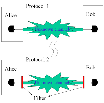
Figure 1: Illustration of protocol 1 and protocol 2, where in protocol 2 finite dimensional filters are put before the detectors. If the filters are properly chosen, the security of protocol 1 can be well approximated by that of protocol 2, while the security of protocol 2 is covered by current information theoretical security proof method. The exact difference between protocol 1 and protocol 2 becomes significant while we consider the the finite key size case.

To simplify our discussion, it is necessary to avoid distinguishing different blocks. We know that $\tilde{D}^{A}-D^{Ai}$ and $\tilde{D}^{B}-D^{Bi}$ are also POVM elements. Here we introduce other two classical data $x^{\prime i}$ and $y^{\prime i}$ that correspond to POVM elements $\tilde{D}^{A}-D^{Ai}$ and $\tilde{D}^{B}-D^{Bi}$ respectively. Then in protocol 1 Alice and Bob’s measurement results of $i$-th block are within the region $\Xi(X^{i})\cup\{x^{\prime i}\}$ and $\Xi(Y^{i})\cup\{y^{\prime i}\}$ respectively. Therefore, this protocol does not change if it runs as follows. While getting measurement results from a state of $i$-th block, Alice and Bob accept them only when they belong to region $\Xi(X^{i})\cup\{x^{\prime i}\}$ and $\Xi(Y^{i})\cup\{y^{\prime i}\}$ respectively. Otherwise, they discard them. Now we can calculate the difference between the protocol 1 and the protocol 2.

III Estimation of $L_{1}$-distance based on observations:

Before calculating the difference, here we introduce a entanglement version measurement. There are several interpretations for the quantum measurement, e.g. von Neumann measurement scheme and Many-worlds interpretation quantum measure . Here we are not to give a new philosophical interpretation, but to construct a physical model that can effectively perform POVM measurement. This physical model allows us to easily find the difference between protocol 1 and protocol 2. For briefness, here we only take Alice’s measurement as an example. Alice’s POVM measurement can be performed by the equipment shown in Fig. 2. The measurement procedure is realized by an interaction among her received state, detector and the environment. After the interaction, Alice gives up received state and the environment and thus only holds the detector, which directly gives her the classical data. After reading out the classical data, Alice set the detector and environment to the initial state to do the next measurement. In this model we require initial states of Alice’s detector and environment are pure and respectively to be $|de\rangle_{A}$ and $|$Env$\rangle_{A}$. For convenience, here we let $|ini\rangle_{A}$ denote $|de\rangle_{A}|$Env$\rangle_{A}$. Then the interaction among the received state, detector and environment for $i$-th block can be given by

$$U_{A}^{i}=\sum_{x^{i}}|x^{i}\rangle|Q_{x^{i}}\rangle_{A}\langle ini|\sqrt{M_{x^{i}}^{Ai}}$$ (3)

where $|x^{i}\rangle$s are orthogonal states of detector, $|Q_{x^{i}}\rangle$ describes orthogonal state of the environment, $\langle ini|$ denotes the initial pure state of Alice’s detector and environment and $\sqrt{M_{x^{i}}^{Ai}}$ is the POVM operators corresponding to POVM element $M_{x^{i}}^{Ai}$ Neilson . To check the validity of this measurement, we can apply it to a two parties system $\rho_{AB}$. After the interaction described by $U_{A}^{i}$, the state of whole system becomes

$$\rho_{ABXQ_{X}} = U_{A}^{i}\rho_{AB}\otimes|ini\rangle_{A}\langle ini|U_{A}^{i+}$$

$$= \sum_{x^{i}}|x^{i}\rangle|Q_{x^{i}}\rangle\sqrt{M_{x^{i}}^{Ai+}}\rho_{AB}\sum_{x^{j}}\langle x^{j}|\langle Q_{x^{j}}|\sqrt{M_{x^{j}}^{Aj}}$$

where $Q_{X}$ denotes the environment and all of $|Q_{x^{i}}\rangle$s are orthogonal with each other. After we trace out the system A and environment we immediately obtain the state

$$\rho_{XB}=\sum_{x^{i}}|x^{i}\rangle\langle x^{i}|\otimes tr_{A}(\sqrt{M_{x^{i}}^{Ai+}}\rho_{AB}\sqrt{M_{x^{i}}^{Ai}})$$

We see that

$$tr_{A}(\sqrt{M_{x^{i}}^{Ai+}}\rho_{AB}\sqrt{M_{x^{i}}^{Ai}})=P(x^{i})\rho_{B}^{x^{i}}$$

where $P(x^{i})$ is the probability of the out come $x^{i}$ and $\rho_{B}^{x^{i}}$ denotes Bob’s conditional state while Alice’s measurement result is $x^{i}$. Then $\rho_{XB}$ becomes

$$\rho_{XB}=\sum_{x^{i}}P(x^{i})|x^{i}\rangle\langle x^{i}|\otimes\rho_{B}^{x^{i}}$$

which consists with the POVM measurement. Since Alice only accept the data within the collection $\Xi(X^{i})\cup\{x^{\prime i}\}$, we can reduce the unitary transformation given in Eq. 3 to a general quantum operation $\hat{O}_{A}^{i}$ to describe Alice’s effective measurement, which is given by

$$\hat{O}_{A}^{i}=\sum_{x^{i}\in\Xi(X^{i})\cup\{x^{\prime i}\}}|x^{i}\rangle|Q_{x^{i}}\rangle_{A}\langle ini|\sqrt{M_{x^{i}}^{Ai}}$$ (4)

Here we can see that $\hat{O}_{A}^{i}$ may not be a unitary transformation. The quantum operation that describes Alice’s total $N$ detection is

$$\hat{O}_{A^{N}}=\bigotimes\limits_{i=1}^{l}(\hat{O}_{A}^{i})^{\otimes n_{i}}$$ (5)

where $n_{i}$ denotes the length of $i$-th block. By the same way we can give the operator describing Bob’s whole $N$ detections (By substituting the notation $A$ by $B$.).

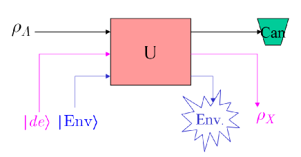
Figure 2: Illustration of entanglement version measurement, where $|$Env$\rangle$ and $|de\rangle$ respectively denote the initial state of environment and the detector. The measurement can be realized by the unitary operation among received state, detector and the environment. After the operation, the received state and the environment are given up and the measurement result can be directly given by the state of detector, denoted by $\rho_{X}$.

Since we only need to consider the case that $\rho_{A^{N}B^{N}E^{N}}$ is pure, here we assume the initial state Alice and Bob receive is $|\Psi_{A^{N}B^{N}E^{N}}\rangle$. The initial state of Alice and Bob’s detector and environment is $|\Psi_{X^{N}Y^{N}Q_{X}^{N}Q_{Y}^{N}}\rangle=|ini\rangle_{A}|ini\rangle_{B}$. Then for the protocol-1, after Alice and Bob’s measurement (general quantum operation Neilson ) the state describing Alice, Bob, Eve, detectors and environment becomes

$$|\Psi_{P-1}\rangle = |\Psi_{X^{N}Y^{N}A^{N}B^{N}Q_{X}^{N}Q_{Y}^{N}E^{N}}\rangle$$ (6)

$$= \frac{\hat{O}_{A^{N}}\hat{O}_{B^{N}}|\Psi_{A^{N}B^{N}E^{N}}\rangle|\Psi_{X^{N}Y^{N}Q_{X}^{N}Q_{Y}^{N}}\rangle}{\sqrt{\langle\hat{O}_{A^{N}}^{+}\hat{O}_{B^{N}}^{+}\hat{O}_{A^{N}}\hat{O}_{B^{N}}\rangle}}$$

where $X$ and $Y$ denotes Alice and Bob’s detectors, $Q_{X}$ and $Q_{Y}$ denote the environment around Alice and Bob, $\hat{O}_{B^{N}}$ is the operator describing Bob’s whole $N$ detections and $\langle\hat{O}_{A^{N}}^{+}\hat{O}_{B^{N}}^{+}\hat{O}_{A^{N}}\hat{O}_{B^{N}}\rangle$ describes expectation value of $\hat{O}_{A^{N}}^{+}\hat{O}_{B^{N}}^{+}\hat{O}_{A^{N}}\hat{O}_{B^{N}}$.

In protocol-2 Alice and Bob respectively put a $d_{A}$ and $d_{B}$ dimensional filter before their detectors. The filter can be described by a projection into a subspace. Here we let the projector $P_{A}^{d_{A}}$ and $P_{B}^{d_{B}}$ denotes Alice and Bob’s filters. For convenience we let $P_{AB}^{d_{A}d_{B}}$ denotes $P_{A}^{d_{A}}\otimes P_{B}^{d_{B}}$. Then for the protocol-2 after Alice and Bob’s measurement the whole state becomes

$$|\Psi_{P-2}\rangle=|\tilde{\Psi}_{X^{N}Y^{N}A^{N}B^{N}Q_{X}^{N}Q_{Y}^{N}E^{N}}\rangle$$ (7)

$$=\frac{\hat{O}_{A^{N}}\hat{O}_{B^{N}}(P_{AB}^{d_{A}d_{B}})^{\otimes N}|\Psi_{A^{N}B^{N}E^{N}}\rangle|\Psi_{X^{N}Y^{N}Q_{X}^{N}Q_{Y}^{N}}\rangle}{\sqrt{\langle(P_{AB}^{d_{A}d_{B}})^{\otimes N}\hat{O}_{A^{N}}^{+}\hat{O}_{B^{N}}^{+}\hat{O}_{A^{N}}\hat{O}_{B^{N}}(P_{AB}^{d_{A}d_{B}})^{\otimes N}\rangle}}$$

After tracing out received quantum state $A^{N}$ and $B^{N}$, and the environment $Q^{N}_{X}$ and $Q^{N}_{Y}$ we obtain the state Alice, Bob and Eve finally hold. For the protocol-1, they finally hold the state $\rho_{X^{N}Y^{N}E^{N}}$ and for the protocol-2, they finally share $\tilde{\rho}_{X^{N}Y^{N}E^{N}}$. If we know the $L_{1}$ distance between $\rho_{X^{N}Y^{N}E^{N}}$ and $\tilde{\rho}_{X^{N}Y^{N}E^{N}}$ we can know the difference between securities of protocol-1 and protocol-2 Renner thesis . Since tracing out the subsystem never increases the $L_{1}$ distance Renner thesis , the $L_{1}$ distance between $\rho_{X^{N}Y^{N}E^{N}}$ and $\tilde{\rho}_{X^{N}Y^{N}E^{N}}$ is no larger than that between $|\Psi_{P-1}\rangle$ and $|\Psi_{P-2}\rangle$. We know that

$$|\Psi_{A^{N}B^{N}E^{N}}\rangle=$$ (8)

$$(P_{AB}^{d_{A}d_{B}})^{\otimes N}|\Psi_{A^{N}B^{N}E^{N}}\rangle+\overline{(P_{AB}^{d_{A}d_{B}})^{\otimes N}}|\Psi_{A^{N}B^{N}E^{N}}\rangle$$

where $\overline{P}$ denotes the orthogonal complement space of $P$. By putting the Eq. (8) into Eq. (6) we quickly know

$$|\Psi_{P-1}\rangle=\alpha|\Psi_{P-2}\rangle+\beta|\Psi^{\prime}\rangle$$

where

$$|\beta|=\frac{\sqrt{\langle\overline{(P_{AB}^{d_{A}d_{B}})^{\otimes N}}\hat{O}_{A^{N}}^{+}\hat{O}_{B^{N}}^{+}\hat{O}_{A^{N}}\hat{O}_{B^{N}}\overline{(P_{AB}^{d_{A}d_{B}})^{\otimes N}}\rangle}}{\sqrt{\langle\hat{O}_{A^{N}}^{+}\hat{O}_{B^{N}}^{+}\hat{O}_{A^{N}}\hat{O}_{B^{N}}\rangle}}.$$ (9)

and

$$|\Psi^{\prime}\rangle=\frac{\hat{O}_{A^{N}}\hat{O}_{B^{N}}\overline{(P_{AB}^{d_{A}d_{B}})^{\otimes N}}|\Psi_{A^{N}B^{N}E^{N}}\rangle|\Psi_{X^{N}Y^{N}Q_{X}^{N}Q_{Y}^{N}}\rangle}{\sqrt{\langle\overline{(P_{AB}^{d_{A}d_{B}})^{\otimes N}}\hat{O}_{A^{N}}^{+}\hat{O}_{B^{N}}^{+}\hat{O}_{A^{N}}\hat{O}_{B^{N}}\overline{(P_{AB}^{d_{A}d_{B}})^{\otimes N}}\rangle}}$$

is a state obtained from the complimentary space $\overline{(P_{AB}^{d_{A}d_{B}})^{\otimes N}}$, which may not be orthogonal with $|\Psi_{P-2}\rangle$. From the Appendix-A of Ref. Renner thesis we know that the $L_{1}$ distance of two pure state $|\Psi_{1}\rangle$ and $|\Psi_{2}\rangle$ can be given by

$$|||\Psi_{1}\rangle-|\Psi_{2}\rangle||=2\sqrt{1-|\langle\Psi_{1}|\Psi_{2}\rangle|^{2}}$$

where $||\cdot||$ denotes the $L_{1}$ distance. Then the $L_{1}$ distance between $|\Psi_{P-1}\rangle$ and $|\Psi_{P-2}\rangle$ is no larger than $2|\beta|$, which yields

$$||\rho_{X^{N}Y^{N}E^{N}}-\tilde{\rho}_{X^{N}Y^{N}E^{N}}||\leq 2|\beta|$$

For convenience here we let $\tilde{D}=\tilde{D}^{A}\tilde{D}^{B}$. If we put Eqs. (4) and (5) into Eq. (9) and apply the fact that operators of different detectors are commutate, we can know that

$$|\beta|=\sqrt{\frac{tr_{ABE}[\tilde{D}^{\otimes N}\overline{(P_{AB}^{d_{A},d_{B}})^{\otimes N}}\rho_{A^{N}B^{N}E^{N}}\overline{(P_{AB}^{d_{A},d_{B}})^{\otimes N}}]}{tr_{ABE}[\tilde{D}^{\otimes N}\rho_{A^{N}B^{N}E^{N}}]}}$$ (10)

Now we can see that if all of pure state $\rho_{A^{N}B^{N}E^{N}}$ satisfying Eq. (2) make $|\beta|$ small enough, then protocol-1 can be well approximated by protocol-2.

To estimate $|\beta|$ here we give a very useful theorem.

Theorem 1

Let $|1\rangle_{A}$, $|2\rangle_{A}$, …, and $|1\rangle_{B}$, $|2\rangle_{B}$, …, be bases of Alice and Bob’s Hilbert spaces respectively, by which projectors $P_{A}^{d_{A}}$ and $P_{B}^{d_{B}}$ can be respectively given by $P_{A}^{d_{A}}=|1\rangle_{A}\langle 1|+...+|d_{A}\rangle_{A}\langle d_{A}|$ and $P_{B}^{d_{B}}=|1\rangle_{B}\langle 1|+...+|d_{B}\rangle_{B}\langle d_{B}|$. Then if we have $\sum_{i=1,j=d_{A}}^{\infty,\infty}|_{A}\langle i|\tilde{D}^{A}|j\rangle_{A}|+\sum_{i=1,j=d_{B}}^{\infty,\infty}|_{B}\langle i|\tilde{D}^{B}|j\rangle_{B}|\leq$ $\frac{\varepsilon^{3}}{N}$, for arbitrary $\rho_{A^{N}B^{N}E^{N}}$ it is always satisfied that $tr_{AB}[\tilde{D}^{\otimes N}\overline{(P_{AB}^{d_{A}d_{B}})^{\otimes N}}\rho_{A^{N}B^{N}}\overline{(P_{AB}^{d_{A}d_{B}})^{\otimes N}}]:=L\leq\varepsilon^{3}$.

Proof: We can see that $L$ is no larger than $\max_{|\Psi^{N}\rangle}\langle\Psi^{N}|\tilde{D}^{\otimes N}|\Psi^{N}\rangle$, where $|\Psi^{N}\rangle\in\overline{(P_{AB}^{d_{A}d_{B}})^{\otimes N}}$. If we expand $\langle\Psi^{N}|\tilde{D}^{\otimes N}|\Psi^{N}\rangle=\langle\Psi^{N}|\overline{(P_{AB}^{d_{A}d_{B}})^{\otimes N}}\tilde{D}^{\otimes N}|\Psi^{N}\rangle$ into product spaces $\overline{P_{A}^{d_{A}}}(P_{A}^{d_{A}})^{\otimes N-1}(P_{B}^{d_{B}})^{\otimes N},...,$ and do straightforward calculation, we can immediately find that $L\leq N[\sum_{i=1,j=d_{A}}^{\infty,\infty}|_{A}\langle i|\tilde{D}^{A}|j\rangle_{A}|+\sum_{i=1,j=d_{B}}^{\infty,\infty}|_{B}\langle i|\tilde{D}^{B}|j\rangle_{B}|]\leq$ $\varepsilon^{3}$. (The straightforward calculation is too bothering to show here. Detailed one can be seen in the appendix.)      $\square$

Since $tr_{ABE}[\tilde{D}^{\otimes N}\rho_{A^{N}B^{N}E^{N}}]\geq\varepsilon$, from Eq. (10), we can see that Theorem 1 actually gives a sufficient condition for $|\beta|\leq\varepsilon$.

Now, we can know the distance between protocol 1 and protocol 2 from the measurement results. The only remained problem is to give the difference between securities of protocol-1 and protocol-2 if the state difference of them is known.

Theorem 2

If $||\rho_{X^{N}Y^{N}E^{N}}-\tilde{\rho}_{X^{N}Y^{N}E^{N}}||\leq 2\delta$ for all $\rho_{A^{N}B^{N}E^{N}}$ satisfying $tr[(\tilde{D}^{A}\tilde{D}^{B})^{\otimes N}\rho_{A^{N}B^{N}E^{N}}]\geq\delta$, then the $5\delta+\epsilon$-secure secret key rate of protocol-1 is no less than the $2\delta+\epsilon$-secure secret key rate of protocol-2, while Alice and Bob take results from protocol-1 as that from protocol-2 to estimate the secret key rate of protocol-2 by the information theoretical method.

Proof: The $L_{1}$ distance cannot be increased by quantum operations and thus classical bit-wise processing Renner thesis . If $||\rho_{X^{N}Y^{N}E^{N}}-\tilde{\rho}_{X^{N}Y^{N}E^{N}}||\leq 2\delta$, then we have $||\rho_{\bar{X}^{k}\bar{E}}-\tilde{\rho}_{\bar{X}^{k}\bar{E}}||\leq 2\delta$ and $||\rho_{X^{N}Y^{N}}-\tilde{\rho}_{X^{N}Y^{N}}||\leq 2\delta$, where $\bar{X}^{k}$, $\bar{Y}^{k}$ and $\bar{E}$ denote Alice and Bob’s classical data and Eve’s state after the data processing respectively, during which some information maybe announced. The security is well defined by smooth min- and max-entropies. The amount of $\epsilon$-secure secret keys can be given by $H_{\min}^{\epsilon^{\prime}}(\rho_{\bar{X}^{k}\bar{E}}|\bar{E})-leak_{IR}$ expl , while the strength of parameter estimation is $\epsilon^{\prime\prime\prime}$, where $H_{\min}^{\epsilon^{\prime}}(\cdot|\cdot)$ denotes the smooth min-entropy, $leak_{IR}$ denotes the amount of information published during the $\epsilon^{\prime\prime}$-secure reconciliation and $\epsilon^{\prime}+\epsilon^{\prime\prime}+\epsilon^{\prime\prime\prime}=\epsilon$ Renner thesis . Since $||\rho_{\bar{X}^{k}\bar{E}}-\tilde{\rho}_{\bar{X}^{k}\bar{E}}||\leq 2\delta$, the smooth min-entropy satisfies $H_{\min}^{2\delta+\epsilon}(\rho_{\bar{X}^{k}\bar{E}}|\bar{E})\geq H_{\min}^{\epsilon}(\tilde{\rho}_{\bar{X}^{k}\bar{E}}|\bar{E})$ Renner thesis . Also, if Alice and Bob use the data from the protocol-1 as that from the protocol-2 to estimate the state of protocol-2, the security of the parameter estimation Renner thesis will be reduced by $2\delta$, because $||\rho_{X^{N}Y^{N}}-\tilde{\rho}_{X^{N}Y^{N}}||\leq 2\delta$. Furthermore, if we only consider the $\rho_{A^{N}B^{N}E^{N}}$ satisfying $tr[(\tilde{D}^{A}\tilde{D}^{B})^{\otimes N}\rho_{A^{N}B^{N}E^{N}}]\geq\delta$, the strength of security will also be reduced by $\delta$. In all, the $\epsilon^{\prime}+\epsilon^{\prime\prime}+\epsilon^{\prime\prime\prime}$ secure security of protocol 2 is given by $H_{\min}^{\epsilon^{\prime}}(\tilde{\rho}_{\bar{X}^{k}\bar{E}}|\bar{E})-leak_{IR}$, while the strength of parameter estimation is $\epsilon^{\prime\prime\prime}$ and the $\tilde{\rho}_{\bar{X}^{k}\bar{E}}$ is estimated by the data obtained from protocol 2. The $\epsilon^{\prime}+\epsilon^{\prime\prime}+\epsilon^{\prime\prime\prime}+2\delta$ secure security of protocol 2 is given by $H_{\min}^{\epsilon^{\prime}}(\tilde{\rho}_{\bar{X}^{k}\bar{E}}|\bar{E})-leak_{IR}$, while the strength of parameter estimation is $\epsilon^{\prime\prime\prime}+2\delta$, where the $\tilde{\rho}_{\bar{X}^{k}\bar{E}}$ is estimated by data obtained from protocol 1. Finally the $\epsilon^{\prime}+\epsilon^{\prime\prime}+\epsilon^{\prime\prime\prime}+5\delta$ secure secret key rate of protocol 1 can be given by $H_{\min}^{2\delta+\epsilon^{\prime}}(\rho_{\bar{X}^{k}\bar{E}}|\bar{E})-leak_{IR}\geq H_{\min}^{\epsilon^{\prime}}(\tilde{\rho}_{\bar{X}^{k}\bar{E}}|\bar{E})-leak_{IR}$, while the strength of parameter estimation is $\epsilon^{\prime\prime\prime}+2\delta$, the state $\tilde{\rho}_{\bar{X}^{k}\bar{E}}$ is estimated by the data obtained from protocol 1 and only the $\rho_{A^{N}B^{N}E^{N}}$ satisfying $tr[(\tilde{D}^{A}\tilde{D}^{B})^{\otimes N}\rho_{A^{N}B^{N}E^{N}}]\geq\delta$ is considered. Here the term $H_{\min}^{\epsilon^{\prime}}(\tilde{\rho}_{\bar{X}^{k}\bar{E}}|\bar{E})-leak_{IR}$ is amount of the $\epsilon^{\prime}+\epsilon^{\prime\prime}+\epsilon^{\prime\prime\prime}+2\delta$ secure secrete keys of protocol 2, while the strength of parameter estimation is $\epsilon^{\prime\prime\prime}+2\delta$, where $2\delta$ comes from the fact that the state $\tilde{\rho}_{\bar{X}^{k}\bar{E}}$ is estimated by the data obtained from protocol 1.           $\square$

The state distance $||\rho_{X^{N}Y^{N}E^{N}}-\tilde{\rho}_{X^{N}Y^{N}E^{N}}||\leq 2\delta$ can be evaluated from the measurement results through theorem 1. The security of protocol 2 is covered by current information theoretical security proof method. Then the the security of protocol 1 can be solved.

IV Security of Protocol 2.

If Alice and Bob’s received initial state in protocol 1 is $\rho_{A^{N}B^{N}}$, the state they received in protocol 2 is $\tilde{\rho}_{A^{N}B^{N}}=\frac{1}{p}(P_{AB}^{d_{A}d_{B}})^{\otimes N}\rho_{A^{N}B^{N}}(P_{AB}^{d_{A}d_{B}})^{\otimes N}$, where $\frac{1}{p}$ is introduced for normalization. After quantum communication, Alice and Bob will permute their state, then $\rho_{A^{N}B^{N}}$ is permutation invariant. The projection operator $(P_{AB}^{d_{A}d_{B}})^{\otimes N}$ commutates with the permutation operator, so $\tilde{\rho}_{A^{N}B^{N}}$ is also a permutation invariant state. The dimension of individual state of $\tilde{\rho}_{A^{N}B^{N}}$ is $d_{A}d_{B}$. Then there is a symmetric purification for $\tilde{\rho}_{A^{N}B^{N}}$ in a Hilbert space of dimension $(d_{A}d_{B})^{2N}$, which actually is $\tilde{\rho}_{A^{N}B^{N}E^{N}}$ Renner thesis ; expl4 . Then the dimension of the individual state of $\tilde{\rho}_{A^{N}B^{N}E^{N}}$ is $(d_{A}d_{B})^{2}$. According to current exponential de Finetti theorem, the state $\tilde{\rho}_{A^{N}B^{N}E^{N}}$ is close to an almost product state expl5 . Then we can only consider the collective attack. Since under the collective attack, Eve attacks all of signals independently by the same method, here we let $\tilde{\rho}_{ABE}$ denotes the state Alice, Bob and Eve share after a single communication. Before calculating the secret key rate, we need to estimate possible $\tilde{\rho}_{ABE}$ from measurement results. It should be noted that although $\tilde{\rho}_{ABE}$ belongs to a Hilbert space of dimension $(d_{A}d_{B})^{2}$, we do not really need to estimate it only in a $(d_{A}d_{B})^{2}$ dimensional subspace. We can still construct it in an infinite dimensional space, because a state belonging to a $(d_{A}d_{B})^{2}$ dimensional Hilbert space also belongs to a infinite dimensional Hilbert space expl2 . This point shows that while we discuss the collective attack for protocol 2, we do not need to take the filter in to account. If we give up filters in protocol 2, the protocol 2 becomes the same as protocol 1. Then if we do not take the filter into account, the security against collective attack of protocol 2 is actually equivalent to that of protocol 1. Finally, our conclusion is as follows. The security of protocol 1 can be approximated by that of protocol 2. For the protocol 2 we only need to consider the collective attack. While the Hilbert space of protocol 2 is only a subspace of protocol 1, then the secrete key rate of protocol 2 against collective attack is no less than that of protocol 1 against collective attack. Finally, we actually give the difference between coherent attack and collective attack for protocol 1. We introduce the filter only to apply current de Finetti theorem and to give the difference between coherent attack and collective attack for protocol 1.

The $5\delta+\epsilon$-secure unconditional secret key rate of protocol-1 is no less than the $2\delta+\epsilon$-secure secret key rate of protocol-2. Under the infinite key size case, the unconditional secrete key rate of protocol 2 is given by the secret key rate against collective attacks Renner thesis . The secret key rate under collective attack of protocol 2 is no less than that of protocol 1. Also under the infinite key size case, the parameter $\epsilon$ can approach to zero. Then the $5\delta$-secure unconditional secret key rate of protocol-1 is no less than the $2\delta$ secure unconditional secret key rate of protocol-2 and no less than its secret key rate against collective attacks, where $2\delta$ comes from the fact that Alice and Bob use the data of protocol 1 to estimate the state of protocol 2. In addition, under the infinite key size case, we may choose large enough $d_{A}$ and $d_{B}$ so as to make $\delta$approach to zero. Then we can directly say that for protocol 1 if the POVM elements corresponding to the measured results can be arbitrarily well described in a finite dimensional space, the collective attack is optimal under the infinite key size case.

For many practical QKDs, the projection of POVM elements of measured results on high dimensional basis is extremely small. For example, the POVM element for heterodyne detection corresponding to measured result $(p,q)$ is $M_{p,q}=\frac{1}{\pi}|p+iq\rangle\langle p+iq|$, whose component on the photon number basis $|m\rangle$ exponentially goes to zero as $m$ increase. The POVM of inefficient photon number resolving detector POVM also has similar property. Then if a QKD protocol utilize such detectors, Alice and Bob can announce the maximum $p^{2}+q^{2}$ or maximum photon number received from one pulse. Then Alice and Bob can construct the big POVM $\tilde{D}$ and for a given $\frac{\varepsilon^{3}}{N}$ they can find a big enough $d$ (smaller than $N$) that in photon number picture satisfies $\sum_{i=1,j=d}^{\infty,\infty}|\langle i|\tilde{D}|j\rangle|\leq$ $\frac{\varepsilon^{3}}{N}$. Then the difference between states of protocol 1 and protocol 2 can be smaller than $2\varepsilon$. The $5\varepsilon+\epsilon$-secure secret key rate can be given by $2\varepsilon+\epsilon$-secure secret key rate of protocol 2, which is covered by Ref. Renner thesis .

V Applications:

In the realistic case, the measured result is always finite. In heterodyne detection protocols, the maximum value of measured result is limited. In photon number detection protocol, the maximum received photon number is finite. Such realistic cases allow us readily apply our results.

Here we give two application examples. We will see that our result can be readily used for heterodyne detection and photon number detection case. It should be noted that in the following we only proved that for CVQKD and DPSQKD the collective attack is optimal under infinite key size case. How to prove their security against collective attack has not been solved in this paper. For short, we only take the infinite key size case for examples. It seems that our estimation of effective dimension is meaningless under this case. However, we should note that under the finite key size case, the estimation of effective dimension will be useful.

V.1 Unconditional security of CVQKD

Now we apply our results to the heterodyne detection CVQKD and prove that as the key size goes to infinite the collective is optimal. In the prepare & measurement CVQKD, Alice prepare a continuous variable EPR pair, and sends one part to Bob. Alice and Bob respectively do heterodyne detection to their held states. The security of such scheme against collective attack is discussed in Ref. binaryCVQKD . Here, we prove that for this protocol the collective attack is optimal under the infinite key size case. We denote Alice and Bob’s measurement result by $(p_{A},q_{A})$ and $(p_{B},q_{B})$ respectively. The corresponding POVM elements are respectively $M_{p_{A},q_{A}}=\frac{1}{\pi}|p_{A}+iq_{A}\rangle\langle p_{A}+iq_{A}|$ and $M_{p_{B},q_{B}}=\frac{1}{\pi}|p_{B}+iq_{B}\rangle\langle p_{B}+iq_{B}|$. In a realistic system, the maximum value of Alice and Bob’s measurement results is finite (or Alice and Bob can give up some extremely larger measurement results). Then their final shared data is within certain region. We assume $V_{A}^{\max}$ and $V_{B}^{\max}$ are large enough, so that for all possible $(p_{A},q_{A})$s and $(p_{B},q_{B})$s Alice and Bob hold satisfy $p_{A}^{2}+q_{A}^{2}\leq V_{A}^{\max}$ and $p_{B}^{2}+q_{B}^{2}\leq V_{B}^{\max}$ (or Alice and Bob only accept the data with amplitude no larger than $V_{A}^{\max}$ and $V_{B}^{\max}$). Then we can construct $\tilde{D}^{A}$ and $\tilde{D}^{B}$ respectively to be

$$\tilde{D}^{A} = \frac{1}{\pi}\int\limits_{p_{A}^{2}+q_{A}^{2}\leq V_{A}^{\max}}|p_{A}+iq_{A}\rangle\langle p_{A}+iq_{A}|dp_{A}dq_{A}$$

$$\tilde{D}^{B} = \frac{1}{\pi}\int\limits_{p_{B}^{2}+q_{B}^{2}\leq V_{A}^{\max}}|p_{B}+iq_{B}\rangle\langle p_{B}+iq_{B}|dp_{B}dq_{B}$$

The filter $P_{A}^{d_{A}}$ and $P_{B}^{d_{B}}$ can be chosen in photon number space. We let

$$P_{A}^{d_{A}} = |0\rangle_{A}\langle 0|+|1\rangle_{A}\langle 1|+...+|d_{A}-1\rangle_{A}\langle d_{A}-1|$$

$$P_{B}^{d_{B}} = |0\rangle_{B}\langle 0|+|1\rangle_{B}\langle 1|+...+|d_{B}-1\rangle_{B}\langle d_{B}-1|$$

where $|i\rangle_{A}\langle i|$ and $|j\rangle_{B}\langle j|$ denote the photon number state. Now we utilize theorem 1 to discuss the difference between protocol 1 and protocol 2. We see that

$$\sum_{i=0,j=d_{A}-1}^{\infty,\infty}|_{A}\langle i|\tilde{D}^{A}|j\rangle_{A}|$$ (11)

$$= \frac{1}{\pi}\int\limits_{p_{A}^{2}+q_{A}^{2}\leq V_{A}^{\max}}\sum_{i=0,j=d_{A}-1}^{\infty,\infty}|_{A}\langle i|p_{A}+iq_{A}\rangle$$

$$\langle p_{A}+iq_{A}|j\rangle_{A}|dp_{A}dq_{A}$$

$$= 2\int\limits_{r_{A}^{2}\leq V_{A}^{\max}}\sum_{i=0,j=d_{A}-1}^{\infty,\infty}\frac{r_{A}^{i}r_{A}^{j}\exp[-r_{A}^{2}]}{\sqrt{i!j!}}dr_{A}$$

$$= 2\int\limits_{r_{A}^{2}\leq V_{A}^{\max}}\sum_{i=0}^{\infty}\frac{r_{A}^{i}\exp[-r_{A}^{2}]}{\sqrt{i!}}\sum_{j=d_{A}-1}^{\infty}\frac{r_{A}^{j}}{\sqrt{j!}}dr_{A}$$

where in the forth line we used the result that $|_{A}\langle i|p_{A}+iq_{A}\rangle|=\frac{r_{A}^{i}\exp[-r_{A}^{2}/2]}{\sqrt{i!}}$ and let $r_{A}^{2}=$ $p_{A}^{2}+q_{A}^{2}$. Under the case that $d_{A}\gg V_{A}^{\max}$, we can use the Stirling formula to approximate $\sqrt{j!}$. Then we have $\sum_{j=d_{A}}^{\infty}\frac{r_{A}^{j}}{\sqrt{j!}}\varpropto(r_{A}/\sqrt{d_{A}})^{d_{A}}$, which exponentially goes to zero as $d_{A}$ increases. Then the whole term $\sum_{i=0,j=d_{A}}^{\infty,\infty}|_{A}\langle i|\tilde{D}^{A}|j\rangle_{A}|$ will exponentially go to zero with the increase of $d_{A}$. By the same way we can prove that the term $\sum_{i=1,j=d_{B}}^{\infty,\infty}|_{B}\langle i|\tilde{D}^{B}|j\rangle_{B}|$ will also exponentially goes to zero with the increase of $d_{B}$. Finally, for a given $\varepsilon^{3}$ and large enough $N$, we can find a $d_{A}\ll N$ and $d_{B}\ll N$, that satisfy

$$\sum_{i=1,j=d_{A}}^{\infty,\infty}|_{A}\langle i|\tilde{D}^{A}|j\rangle_{A}|+\sum_{i=1,j=d_{B}}^{\infty,\infty}|_{B}\langle i|\tilde{D}^{B}|j\rangle_{B}|:=Err\leq\ \frac{\varepsilon^{3}}{N}$$

Then from the theorem 1 and 2 we know that the security of this CVQKD scheme can be approximated by the security of a scheme of dimension $(d_{A}d_{B})^{2}\ll N$ with errors no larger than $5\varepsilon$ ($Err$ exponentially approach to zero with the increase of $d_{A}$ and $d_{B}$, so that $d_{A}$ and $d_{B}$ are proportional with $\log(N/\varepsilon^{3})$. Then for large enough $N$, we can have $(d_{A}d_{B})^{2}\ll N$). Then $5\varepsilon+\epsilon$-secure secret key rate of heterodyne detection CVQKD can be given by $2\varepsilon+\epsilon$-secure secret key rate of protocol-2, where Alice and Bob respectively put filters $P_{A}^{d_{A}}$ and $P_{B}^{d_{B}}$ before their detectors. As $N\rightarrow\infty$, we can find large enough $(d_{A}d_{B})^{2}\ll N$, that allow $\varepsilon\rightarrow 0$, and the security parameter $\epsilon$ can goes to zero From the Ref. Renner thesis we know that, under the case that $(d_{A}d_{B})^{2}\ll N\rightarrow\infty$, the collective attack is optimal for protocol 2 and its secret key rate can be given by that under collective attack. Since the secrete key rate against collective attack of protocol 2 is no larger than that of protocol 1, under the infinite key size case the unconditional secret key rate of heterodyne detection CVQKD equal to its secret key rate under collective attacks and the collective is optimal. Here, we require Alice and Bob give up such data whose amplitude is larger than $V_{A}^{\max}$ and $V_{B}^{\max}$. We can expect that for large $V_{A}^{\max}$ and $V_{B}^{\max}$, the proportion of given up data is extremely small. Such procedure only causes extremely small change of state, and thus only cause extremely small change of security. On the other hand, a realistic security proof for CVQKD should take such cut off procedure into account. After all, in a realistic situation, the maximum value of measurement results is always finite.

V.2 Unconditional security of DPSQKD

Now we apply our result to coherent state DPSQKD, whose dimension is infinite in principle. Up to now, the security against collective attack for DPSQKD under noiseless case is proved DPSQKD . Here we show that that proof actually is unconditional security proof. To allow Alice and Bob do random permutation, in Ref. DPSQKD Zhao et al. cut the long sequence of coherent states into blocks and regarded one block as one big state. Then Alice and Bob can permute these big states. In the DPSQKD Alice sends Bob a big state $|\Psi_{\vec{x}}^{N_{b}}\rangle={\bigotimes\limits_{i=1}^{N_{b}}}|(-1)^{x_{i}+1}\alpha\rangle$ (denotes the state of a block), according to her binary string $\vec{x}=(x_{1},x_{2},...,x_{N_{b}})$, where $|(-1)^{x_{i}+1}\alpha\rangle$ is a coherent state. Then Bob measures the phase difference between each two individual state. The collective attack means Eve attack these big states (blocks) independently with the same method. Here we require Bob use the photon number resolving detector. After many rounds of quantum communications, Bob announces the maximum photon number received from one big state (one block). Then if Bob put a filter that filters out all the state whose photon number is larger than certain criteria, the measured results should not change too much.

We see that if the efficiency of photon number resolving detector is 100%, then we can definitely know the actual dimension of Bob’s received state. However, if that efficiency is not 100%, we cannot determine the exact dimension of Bob’s state from the measured photon numbers.

Here we discuss the imperfect detector case. In Ref. POVM2 , the POVM element of ineffective photon number resolving detector is given. In that reference, the spacial mode of received photon state has not been considered. If we take the spacial mode and other components into account, we can extend that POVM element corresponding to $n$ photons to be

$$\Pi_{n}=\sum\limits_{m=n}^{\infty}C^{n}_{m}\gamma^{n}(1-\gamma)^{m-n}P_{m}$$ (12)

where $\gamma$ denotes detector efficiency and $P_{m}$ denotes the projector to $m$ photon number subspace. We assume the dimension of $m$ photon number subspace is $f_{m}$, and $P_{m}$ to be

$$P_{m}=\sum_{k=1}^{f_{m}}|\varphi_{k}^{m}\rangle\langle\varphi_{k}^{m}|$$ (13)

where $|\varphi_{k}^{m}\rangle$ denotes the orthogonal state of $m$ photon number subspace. It can be prove that $f_{m}\leq l(m+l-1)!/m!$, where $l$ denotes the block size.

If Bob’s maximum received photon number is $n_{0}$, then the POVM element corresponding to this event can be given by

$$\tilde{D}^{B}=\sum_{n=0}^{n=n_{0}}\Pi_{n}$$ (14)

In DPSQKD, if the block size is $l$, the dimension of Alice’s modulation is $2^{l}$, which is finite. Therefore we only need to discuss Bob’s state. We can construct Bob’s filter to be

$$P_{B}^{d_{B}}=\sum_{m=0}^{m=m_{0}}P_{m}$$

where $P_{m}$ is given by Eq. (13). Now we can use theorem 1 to estimate the difference between protocol 1 and protocol 2. We enumerate the basis of the filter by $|\varphi_{k}^{m}\rangle$. Then we have

$$Diff:=\sum_{m=0,m^{\prime}=m_{0},k,k^{\prime}}\langle\varphi_{k}^{m}|\tilde{D}^{B}|\varphi_{k^{\prime}}^{m^{\prime}}\rangle$$ (15)

$$\leq\sum_{n=0}^{n_{0}}\gamma^{n}\sum_{m=m_{0}}C_{m}^{n}(1-\gamma)^{m-n}l(m+l-1)!/m!$$

$$\leq\sum_{n=0}^{n_{0}}\gamma^{n}\sum_{m=m_{0}}(1-\gamma)^{m-n}l/n!(m+l-1)^{l+n-1}$$

where in the second line we have used Eqs. (12), (13) and (14) and the fact that $f_{m}\leq l(m+l-1)!/m!$ and in the third line we used the fact that $m(m-1)...(m-n)\leq m^{n}$. It can be seen that $Diff$ exponentially goes to zero as $m_{0}$ increases. Then for a given security parameter we can find a large enough key size $N$ that gives the required security.

It also can be seen that if Bob use the perfect photon number resolving detector or a detector that can given the upper bound of the number of received photons (e.g. bourn up if received photon number is too high), then they can find a protocol 2 that is exactly same as protocol 1. Then we can immediately get a conclusion that the collective attack is optimal under the infinite key size case.

VI Conclusion:

In the above we give a method to apply current exponential de Finetti theorem to realistic QKD. In realistic QKD, the number of Alice and Bob received photons is always finite and their measurement results always belong to a finite region. This property allow us effectively describe the QKD protocol in a finite dimensional subspace with sufficiently small error. In this paper, we introduce another finite dimensional protocol by putting finite dimensional filters before the detectors, and shown the security difference between the original unknown-dimensional protocol and this finite dimensional protocol based on measurement results. Since the security of that finite dimensional protocol is covered by current information theoretical security proof method, the security of a realistic unknown dimensional system can be solved. Our result can be used to prove the unconditional security of heterodyne detection CVQKD and DPSQKD. Finally, we prove that for heterodyne detection CVQKD and DPSQKD collective attack is optimal under the infinite key size case. The difference between protocol 1 and protocol 2 will be meaningful if we consider the finite key size case.

Acknowledgement: Special thanks are given to R. Renner for fruitful discussions. This work is supported by National Natural Science Foundation of China under Grants No. 60537020 and 60621064.

Appendix A Detailed proof for Theorem 1

At first we can see that $tr_{AB}[\tilde{D}^{\otimes N}\overline{(P_{AB}^{d_{A}d_{B}})^{\otimes N}}\rho_{A^{N}B^{N}}\overline{(P_{AB}^{d_{A}d_{B}})^{\otimes N}}]$ is no larger than $\max_{|\Psi^{N}\rangle}\langle\Psi^{N}|\tilde{D}^{\otimes N}|\Psi^{N}\rangle$ where $|\Psi^{N}\rangle\in\overline{(P_{AB}^{d_{A}d_{B}})^{\otimes N}}$. To find $\max_{|\Psi^{N}\rangle}\langle\Psi^{N}|\tilde{D}^{\otimes N}|\Psi^{N}\rangle$, we need to expand the space $\overline{(P_{AB}^{d_{A}d_{B}})^{\otimes N}}$ by product spaces $\overline{P_{A}^{d_{A}}}(P_{A}^{d_{A}})^{\otimes N-1}(P_{B}^{d_{B}})^{\otimes N},...$. Here, we let $P_{A_{k}}^{d_{A}}$ ($P_{B_{k}}^{d_{B}}$) denote the projector to Alice’s (Bob’s) $k$-th state. Also we distinguish bases of $k$-th state of Alice (Bob) as $|1\rangle_{A_{k}},|2\rangle_{A_{k}},...$, ($|1\rangle_{B_{k}},|2\rangle_{B_{k}},...$). We know that $I_{A_{k}}=P_{A_{k}}^{d_{A}}+\overline{P_{A_{k}}^{d_{A}}}$ and $I_{B_{k}}=P_{B_{k}}^{d_{A}}+\overline{P_{B_{k}}^{d_{A}}}$, where $I_{A_{k}}$ and $I_{B_{k}}$ are the identity matrixes corresponding to Alice and Bob’s $k$-th states. Then we have

$$\langle\Psi^{N}|\tilde{D}^{\otimes N}|\Psi^{N}\rangle=\langle\Psi^{N}|(P_{A_{1}}^{d_{A}}+\overline{P_{A_{1}}^{d_{A}}})\tilde{D}^{\otimes N}|\Psi^{N}\rangle$$

$$=\langle\Psi^{N}|\overline{P_{A_{1}}^{d_{A}}}\tilde{D}^{\otimes N}|\Psi^{N}\rangle+\langle\Psi^{N}|P_{A_{1}}^{d_{A}}\tilde{D}^{\otimes N}|\Psi^{N}\rangle$$

$$=C_{F}^{1}+C_{L}^{1}$$ (16)

where $C_{F}^{1}$ and $C_{L}^{1}$ respectively denote the first and second term in the second line. Since

$$\begin{array}[]{c}\overline{P_{A_{1}}^{d_{A}}}=|d_{A}+1\rangle_{A_{1}}\langle d_{A}+1|+|d_{A}+2\rangle_{A_{1}}\langle d_{A}+2|+...\\ I_{A_{1}}=|1\rangle_{A_{1}}\langle 1|+|2\rangle_{A_{1}}\langle 2|+...\end{array}$$

the $C_{F}^{1}$ can be given by

$$C_{F}^{1} = \langle\Psi^{N}|\overline{P_{A_{1}}^{d_{A}}}\tilde{D}^{\otimes N}I_{A_{1}}|\Psi^{N}\rangle$$

$$= \sum_{m_{1}=d_{A}+1,m_{1}^{\prime}=1}^{\infty,\infty}\langle m_{1}|\tilde{D}^{A}|m_{1}^{\prime}\rangle\cdot$$

$$\langle\Psi^{N}|m_{1}\rangle(\tilde{D}^{A})^{\otimes N-1}(\tilde{D}^{B})^{\otimes N}\langle m_{1}^{\prime}|\Psi^{N}\rangle$$

where we have used the fact that $P_{A_{k}}^{d_{A}}$ and $\tilde{D}_{j}^{A}$ and $\tilde{D}_{j}^{B}$ are commutate if $k\neq j$ and $\tilde{D}_{j}^{A}$ and $\tilde{D}_{j}^{B}$ denote POVM elements corresponding to $j$-th state. We know there exist two pure states $|\Phi_{1}^{m_{1}}\rangle$ and $|\tilde{\Phi}_{1}^{m_{1}^{\prime}}\rangle$ that can let $\langle m_{1}^{\prime}|\Psi^{N}\rangle$ and $\langle m_{1}|\Psi^{N}\rangle$ be written as $\langle m_{1}|\Psi^{N}\rangle=\lambda_{1}|\Phi_{1}^{m_{1}}\rangle$ and $\langle m_{1}^{\prime}|\Psi^{N}\rangle=\lambda_{1}^{\prime}|\tilde{\Phi}_{1}^{m_{1}^{\prime}}\rangle$, where $|\lambda_{1}|\leq 1$ and $|\lambda_{1}^{\prime}|\leq 1$. Then $C_{F}^{1}$ can be given by

$$C_{F}^{1} = \langle\Psi^{N}|\overline{P_{A_{1}}^{d_{A}}}\tilde{D}^{\otimes N}I_{A_{1}}|\Psi^{N}\rangle$$

$$= \lambda_{1}\lambda_{1}^{\prime}\sum_{m_{1}=d_{A}+1,m_{1}^{\prime}=1}^{\infty,\infty}\langle m_{1}|\tilde{D}^{A}|m_{1}^{\prime}\rangle\cdot$$

$$\langle\Phi_{1}^{m_{1}}|(\tilde{D}^{A})^{\otimes N-1}(\tilde{D}^{B})^{\otimes N}|\tilde{\Phi}_{1}^{m_{1}^{\prime}}\rangle$$

Before giving the upper bound to $C_{F}^{1}$, we will discuss the upper bound of $|\langle\Phi_{1}^{m_{1}}|(\tilde{D}^{A})^{\otimes N-1}(\tilde{D}^{B})^{\otimes N}|\tilde{\Phi}_{1}^{m_{1}^{\prime}}\rangle|$. It is known that arbitrary POVM element $M$ can be written into a diagonal form. We assume an arbitrary $M$ can be written as

$$M=a_{1}|\varphi_{1}\rangle\langle\varphi_{1}|+a_{2}|\varphi_{2}\rangle\langle\varphi_{2}|+...$$

where $|\varphi_{1}\rangle,|\varphi_{2}\rangle,...$are orthogonal bases, and $a_{1},a_{2},...$ are positive real numbers and satisfy $a_{i}\leq 1$. We let $|\psi\rangle$ and $|\psi^{\prime}\rangle$ are two arbitrary states. Now we consider the following value for $|\psi\rangle$ and $|\psi^{\prime}\rangle$.

$$|\langle\psi|M|\psi^{\prime}\rangle|=|a_{1}\langle\psi|\varphi_{1}\rangle\langle\varphi_{1}|\psi^{\prime}\rangle+a_{2}\langle\psi|\varphi_{2}\rangle\langle\varphi_{2}|\psi^{\prime}\rangle+...|$$

From the fact that

$$|\langle\psi|\varphi_{1}\rangle|^{2}+|\langle\psi|\varphi_{2}\rangle|^{2}+... \leq 1$$ (19)

$$|\langle\psi^{\prime}|\varphi_{1}\rangle|^{2}+|\langle\psi^{\prime}|\varphi_{2}\rangle|^{2}+... \leq 1$$

we know that for arbitrary states $|\psi\rangle$ and $|\psi^{\prime}\rangle$ and POVM element $M$, it is always satisfied that

$$|\langle\psi|M|\psi^{\prime}\rangle| \leq \sqrt{|a_{1}\langle\psi|\varphi_{1}\rangle|^{2}+|a_{2}\langle\psi|\varphi_{2}\rangle|^{2}+...}$$

$$\leq \sqrt{|\langle\psi|\varphi_{1}\rangle|^{2}+|\langle\psi|\varphi_{2}\rangle|^{2}+...}\leq 1$$

where in the first line we applied the Cauchy-Schwartz inequality which says that

$$|a_{1}b_{1}+a_{2}b_{2}+...|\leq$$

$$\sqrt{|a_{1}|^{2}+|a_{2}|^{2}+...}\sqrt{|b_{1}|^{2}+|b_{2}|^{2}+...}$$

and in the second line we applied Eq. (19) and the fact that $a_{i}\leq 1$.

Now we put Eq. (A) into Eq. (A) and obtain

$$|C_{F}^{1}|\leq\sum_{m_{1}=d_{A}+1,m_{1}^{\prime}=1}^{\infty,\infty}|\langle m_{1}|\tilde{D}^{A}|m_{1}^{\prime}\rangle|$$ (21)

By the same way $C_{L}^{1}$ can be given by

$$C_{L}^{1} = \langle\Psi^{N}|P_{A_{1}}^{d_{A}}\tilde{D}^{\otimes N}|\Psi^{N}\rangle$$

$$= \langle\Psi^{N}|P_{A_{1}}^{d_{A}}\overline{P_{A_{2}}^{d_{A}}}\tilde{D}^{\otimes N}|\Psi^{N}\rangle+\langle\Psi^{N}|P_{A_{1}}^{d_{A}}P_{A_{2}}^{d_{A}}\tilde{D}^{\otimes N}|\Psi^{N}\rangle$$

$$= C_{F}^{2}+C_{L}^{2}$$

where $C_{F}^{2}$ and $C_{L}^{2}$ respectively denote the first and the second term in the second line.

As the $C_{F}^{1}$, the $C_{F}^{2}$ can be rewritten as

$$C_{F}^{2} = \langle\Psi^{N}|P_{A_{1}}^{d_{A}}\overline{P_{A_{2}}^{d_{A}}}\tilde{D}^{\otimes N}I_{A_{2}}|\Psi^{N}\rangle$$ (22)

$$= \sum_{m_{2}=d_{A}+1,m_{2}^{\prime}=1}^{\infty,\infty}\langle m_{2}|\tilde{D}^{A}|m_{2}^{\prime}\rangle\cdot$$

$$\langle\Psi^{N}|m_{2}\rangle P_{A_{1}}^{d_{A}}(\tilde{D}^{A})^{\otimes N-1}(\tilde{D}^{B})^{\otimes N}\langle m_{2}^{\prime}|\Psi^{N}\rangle$$

Also there exist a pure state $|\Phi_{2}^{m_{2}}\rangle$ by which $\langle\Psi^{N}|m_{2}\rangle P_{A_{1}}^{d_{A}}$ can be written as $\lambda_{2}\langle\Phi_{2}^{m_{2}}|$ and a pure state $|\tilde{\Phi}_{2}^{m_{2}^{\prime}}\rangle$ by which $\langle m_{2}^{\prime}|\Psi^{N}\rangle$ can be given by $\lambda_{2}^{\prime}|\tilde{\Phi}_{2}^{m_{2}^{\prime}}\rangle$. Since $|\lambda_{1}|\leq 1$ and $|\lambda_{2}|\leq 1$, from the Eqs. (A) and (22) we know that

$$|C_{F}^{2}|\leq\sum_{m_{2}=d_{A}+1,m_{2}^{\prime}=1}^{\infty,\infty}|\langle m_{2}|\tilde{D}^{A}|m_{2}^{\prime}\rangle|$$ (23)

If we continuously do such procedure, we will find that

$$\langle\Psi^{N}|(\tilde{D}^{A}\tilde{D}^{B})^{\otimes N}|\Psi^{N}\rangle=\sum_{i=1}^{2N}C_{F}^{i}+C_{L}^{2N}$$ (24)

and

$$|C_{F}^{i}|\leq\sum_{m_{i}=d_{A}+1,m_{i}^{\prime}=1}^{\infty,\infty}|\langle m_{i}|\tilde{D}^{A}|m_{i}^{\prime}\rangle|$$ (25)

for $i\leq N$, and

$$|C_{F}^{i}|\leq\sum_{m_{i}=d_{B}+1,m_{i}^{\prime}=1}^{\infty,\infty}|\langle m_{i}|\tilde{D}^{B}|m_{i}^{\prime}\rangle|$$ (26)

for $i>N$, where

$$C_{L}^{2N}=\langle\Psi^{N}|(P_{AB}^{d_{A}d_{B}})^{\otimes N}\tilde{D}^{\otimes N}|\Psi^{N}\rangle=0$$ (27)

and we have applied the fact that $|\Psi^{N}\rangle\in$ $\overline{(P_{AB}^{d_{A}d_{B}})^{\otimes N}}$. Finally from Eqs. (24), (25) (26) and (27) we can see that

$$|\langle\Psi^{N}|\tilde{D}^{\otimes N}|\Psi^{N}\rangle|\leq\sum_{i=1}^{2N}|C_{F}^{i}|$$ (28)

$$\leq N[\sum_{i=1,j=d_{A}}^{\infty,\infty}|_{A}\langle i|\tilde{D}^{A}|j\rangle_{A}|+\sum_{i=1,j=d_{B}}^{\infty,\infty}|_{B}\langle i|\tilde{D}^{B}|j\rangle_{B}|]$$

Since Eq. (28) holds for arbitrary $|\Psi^{N}\rangle\in\overline{(P_{AB}^{d_{A}d_{B}})^{\otimes N}}$, the Theorem 1 is proved.

References

• (1) R. Renner, aXiv: quant-ph/0512258 (2005).
• (2) M. Christandl, R. Koenig, G. Mitchison, R. Renner, Comm. Math. Phys. 273, 473 (2007).
• (3) M. Christandl and B. Toner, arXiv:0712.0916 (2007).
• (4) C. D́Cruz, T. J. Osborne, R. Schack, Phys. Rev. Lett. 98, 160406 (2007).
• (5) R. Renner, Nature Physics 3, 645 (2007).
• (6) T. Tsurumaru, K. Tamaki, Phys. Rev. A 78, 032302 (2008).
• (7) N. J. Beaudry, T. Moroder and N. Lütkenhaus, Phys. Rev. Lett. 101, 093601 (2008).
• (8) Y.-B. Zhao, M. Heid, J. Rigas, N. Lütkenhaus, Phys. Rev. A 79, 012307 (2009).
• (9) R. Garcia-Patron and N. J. Cerf, Phys. Rev. Lett. 97, 190503 (2006).
• (10) Y.-B. Zhao, C.-H. F. Fung, Z.-F. Han and G.-C. Guo, Phys. Rev. A 78, 042330 (2008).
• (11) S. Wehner, M. Christandl, A. C. Doherty, arXiv:0808.3960 (2008).
• (12) Y.-B. Zhao, Y.-Z. Gui, J.-J. Chen, Z.-F. Han, G.-C. Guo IEEE Trans. Inform. Theory, 54, 2803 (2008).
• (13) V. Scarani and R. Renner, Phys. Rev. Lett. 100, 200501 (2008).
• (14) R. Renner and J. I. Cirac, arXiv: 0809.2243 (2008).
• (15) A. Leverrier, E. Karpov, P. Grangier and N. J. Cerf, arXiv:0809.2252 (2008).
• (16) M. A. Nielsen and I. L. Chuang, Quantum Computing and Quantum Information, (Cambridge University Press,Cambridge, UK, 2000).
• (17) From the definition of the universal security, we know $\varepsilon$-secure key can be considered indentical to an ideal key, except with probability $\varepsilon$ Renner thesis .
• (18) V. B. Braginsky and F. Y. Khalili, Quantum Measurement, Camebridge University Press, (1992).
• (19) Here we omit a small term proportional to $O[\text{log}(1/\epsilon^{\prime})]$.
• (20) There may be many different purifications, but all of them are different by local unitary transformations at Eve’s side. The local unitary transformation does not change the smooth min-entropy. Therefore, all purifications are equivalent actually.
• (21) Here we assume $(d_{A}d_{B})^{2}\ll N$
• (22) Under the collective attack, the secret key rate can be given by $\min_{\tilde{\rho}_{ABE}\in\Xi(\tilde{\rho}_{ABE})}H(X|E)-leak_{IR}$, where $\Xi(\tilde{\rho}_{ABE})$ is the collection of all $\tilde{\rho}_{ABE}$s (in a finite dimensional space) that consist with the observation. If we define a collection $\Xi(\rho_{ABE})$ to denote the collection of $\rho_{ABE}$s (belong to a infinite dimensional space) that consist with the observation, we can find that $\Xi(\tilde{\rho}_{ABE})\in\Xi(\rho_{ABE})$. Therefore we have $\min_{\tilde{\rho}_{ABE}\in\Xi(\tilde{\rho}_{ABE})}H(X|E)\geq\min_{\rho_{ABE}\in\Xi(\rho_{ABE})}H(X|E)$. This inequality means that the secret key rate against the collective attack of protocol 2 is no less than that of protocol 1.
• (23) A. M. Branczyk, T. J. Osborne, A. Gilchrist and T. C. Ralph. Phys. Rev. A 68, 043821 (2003).
• (24) S. D. Bartlett, E. Diamanti, B. C. Sanders, and Y. Yamamoto, arXiv:quant-ph/0204073 (2002).