Derivation of Green’s Function of Spin Calogero-Sutherland Model
by Uglov’s Method

Abstract

Hole propagator of spin $1/2$ Calogero-Sutherland model is derived using Uglov’s method, which maps the exact eigenfunctions of the model, called Yangian Gelfand-Zetlin basis, to a limit of Macdonald polynomials (gl₂-Jack polynomials). To apply this mapping method to the calculation of 1-particle Green’s function, we confirm that the sum of the field annihilation operator $\hat{\psi}_{\uparrow}+\hat{\psi}_{\downarrow}$ on Yangian Gelfand-Zetlin basis is transformed to the field annihilation operator $\hat{\psi}$ on gl₂-Jack polynomials by the mapping. The resultant expression for hole propagator for finite-size system is written in terms of renormalized momenta and spin of quasi-holes and the expression in the thermodynamic limit coincides with the earlier result derived by another method. We also discuss the singularity of the spectral function for a specific coupling parameter where the hole propagator of spin Calogero-Sutherland model becomes equivalent to dynamical colour correlation function of SU(3) Haldane-Shastry model.

1 Introduction

Calogero-Sutherland model[1, 2, 3, 4, 5, 6, 7, 8, 9] is a one-dimensional quantum system of particles with two-body interaction inversely proportional to the square of distance. From theoretical point of view, Calogero-Sutherland model has attracted extensive attention in relation to fractional exclusion statistics[10, 11, 12], Jack polynomials[13, 14], Tomonaga-Luttinger liquid[15], collective field theory[16, 17] and matrix models[18]. An intriguing property of Calogero-Sutherland model lies in the fact that exact expressions of two-point dynamical correlation functions have been obtained for whole range of time and space[18, 19, 20, 21, 22, 23, 24, 25, 26, 27]. The expressions for dynamical correlation functions are much simpler than those of Bethe solvable models[28]. Through exact explicit expressions of spectral functions of Calogero-Sutherland model, dynamical properties of one-dimensional quantum systems have been discussed[29, 30].

In this paper, we consider spin generalization of Calogero-Sutherland model[31, 32, 33], which is the model of particles with spin 1/2 as internal degrees of freedom. In the following we call this model “spin Calogero-Sutherland model” while the original model “scalar Calogero-Sutherland model”. Spin Calogero-Sutherland models are even more important than scalar model in the sense that (i) the spin Calogero-Sutherland models have Yangian symmetry[34, 35] as an internal symmetry, (ii) it reduces to the Haldane-Shastry model[36, 37] in the limit of infinite coupling parameter[38, 39] and (iii) it realizes the Tomonaga-Luttinger liquid (of particles with spin internal symmetry) in the systems with finite number of particles in the simplest manner[32, 40].

Exact results of dynamical correlation functions such as hole propagator[41, 42], density correlation[43, 44] and spin correlation function[43, 44, 45, 46] have been obtained in spin Calogero-Sutherland model. However particle propagator of this model has not been derived. With knowledge of hole and particle propagators, we can arrive at full understanding of the dynamics and elementary excitations. From the hole and particle propagators, furthermore, we can construct 1-particle causal Green’s function, which provides a nontrivial starting point of many-body perturbation theory. The derivation of exact results applicable both to hole and particle propagators, therefore, is highly required from the above point of view. We address this issue in the present paper.

There are two types of the expression of the wave functions of the spin Calogero-Sutherland model. The first one is given by Jack polynomial with prescribed symmetry[47, 48]. This polynomial is constructed by partially symmetrization or anti-symmetrization of non-symmetric Jack polynomials[49, 50], which are the simultaneous eigenfunctions of the integrals of motion of this model, that is Cherednik-Dunkl operators[51, 52]. Jack polynomials with prescribed symmetry form an orthogonal basis of the Hilbert space with a specific spin configuration. The second one is related to the Yangian symmetry[34, 35] of spin Calogero-Sutherland model. An orthogonal basis of the Fock space including spin degrees of freedom with fixed particle number is called Yangian Gelfand-Zetlin basis[53, 54]

Dynamical correlation functions of spin Calogero-Sutherland model were calculated in two methods according to the two types of eigenfunctions. One way uses Jack polynomials with prescribed symmetry as eigenfunctions, and the dynamical correlation functions are calculated by using the relations derived from the non-symmetric Jack polynomials. With this method, hole propagator [41, 42] has been derived by one of the authors and his collaborator. Recently[55], it was found that dynamical density correlation of spin Calogero-Sutherland model can be derived with Jack polynomials with prescribed symmetry and the method used in [56]. However, no formulas necessary to particle propagator have been obtained in the theory of Jack polynomials with prescribed symmetry.

The other way uses Yangian Gelfand-Zetlin basis as eigenfunctions together with the mapping from Yangian Gelfand-Zetlin basis to symmetric polynomials[43]. The relations of this polynomial necessary to calculate dynamical correlation function are derived from those of Macdonald polynomials[14]. Density correlation function and spin correlation function have been derived with this method[43, 44]. We refer to the latter method as Uglov’s method. For a decade, it has been unresolved issue whether the Uglov’s method is applicable to the calculation of 1-particle Green’s function. In Uglov’s method, wavefunctions of multi-component particles are mapped to those of single-component particles. It is not obvious how the field operator in 1-particle Green’s function is transformed under this mapping, in contrast to the density operator or spin operator considered in [43].

The main purpose of this paper is to show that Uglov’s method is applicable to derive both hole and particle propagators. More explicitly, we give the transformation of field operator under the Uglov’s mapping from multi-component system to single-component one. As an application, hole propagator is calculated by using this method. With introducing renormalized momenta and spin variables of quasi-holes, the expression for hole propagator in finite-sized system becomes much simpler than that derived in [42]. We confirm that the expression in the thermodynamic limit recovers the earlier result[42]. Furthermore we discuss spectral function of hole propagator for a specific coupling constant ($\lambda=1$ in the notations we will introduce in the following chapters). At this coupling parameter, the hole propagator of spin Calogero-Sutherland model is equivalent to the dynamical colour correlation function[45, 46] of SU(3) Haldane-Shastry model[31, 32, 57] as shown by Arikawa[58]. In the same way as hole propagator, particle propagator can be mapped to that of single-component model. However, it is more involved to take the thermodynamic limit of particle propagator than hole propagator. Therefore, we report the calculation of particle propagator and discussion of the corresponding spectral weight in a separate paper.

To outline this paper, the basic properties of Spin Calogero-Sutherland model are shown in section 2. In section 3, the mapping of the field annihilation operator is considered. Using the result of section 3, hole propagator of spin Calogero-Sutherland model is derived in section 4. The expression for hole propagator is rewritten in terms of quasi-hole rapidities in section 5. The properties of the spectral function for $\lambda=1$ are discussed in section 6.

2 Basic Properties

In this section, we review the basic properties of spin Calogero-Sutherland model.

2.1 Hamiltonian and eigenfunctions

Spin Calogero-Sutherland model is a one-dimensional quantum model which consists of $N$ particles with spin degrees of freedom, moving along the circle of perimeter $L$. Each pair of particles has an interaction of inverse square type potential. Hamiltonian is given by

$$H=-\sum_{i=1}^{N}\frac{\partial^{2}}{\partial x_{i}^{2}}+\frac{2\pi^{2}}{L^{2}}\sum_{i<j}\frac{\lambda(\lambda+P_{ij})}{\displaystyle\sin^{2}\left[\pi(x_{i}-x_{j})/L\right]},$$ (1)

where $x_{i}$ is the coordinate of $i$-th particle, and $P_{ij}$ is the spin exchange operator for particles $i$ and $j$. The Hamiltonian (1) has one parameter, an interaction parameter $\lambda$, which controls whole physical properties of the system. Physically, $\lambda<0$ is unrealistic due to the collapse of the particles. In the following of this paper, we consider particles with spin 1/2, and $\lambda$ is restricted to be non-negative integer for simplicity.

Let the particles be bosons for odd $\lambda$ and fermions for even $\lambda$, following to the earlier works on the hole propagator[41, 42], and the boundary condition is chosen to be periodic. In the ground state, $N/2$ is taken to be odd (even) when $\lambda$ is even (odd) to avoid the degeneracy of the ground state. Introducing new variables $z=\{z_{1},\cdots,z_{N}\}$ with $z_{i}=\exp[2\pi\rmi x_{i}/L]$, the wave function $\Psi(\{x_{i}\},\{\sigma_{i}\})$ for spin $1/2$ model is written as the product $\Phi(z,\sigma)\Psi_{0,N}(z)$ of Jastrow type wave function

$$\Psi_{0,N}(z)=\prod_{i}z_{i}^{-\lambda(N-1)/2}\prod_{i<j}(z_{i}-z_{j})^{\lambda}$$ (2)

and a function $\Phi(z,\sigma)$ of complex spatial coordinates $z$ and spin variables $\sigma=\{\sigma_{1},\cdots,\sigma_{N}\}$. The spin coordinate $\sigma_{i}$ takes 1 (2) for spin up (spin down).

When $\lambda$ is even, particles are fermions and the Jastrow wave function $\Psi_{0,N}(z)$ is symmetric with respect to interchange of $z_{i}$ and $z_{j}$. $\Phi(z,\sigma)$ then obeys the fermionic Fock condition,

$$\Phi(\cdots,z_{i},\sigma_{i},\cdots,z_{j},\sigma_{j},\cdots)=-\Phi(\cdots,z_{j},\sigma_{j},\cdots,z_{i},\sigma_{i},\cdots).$$ (3)

When $\lambda$ is odd, on the other hand, the particles are bosons and the Jastrow wave function $\Psi_{0,N}(z)$ is anti-symmetric with respect to interchange of $z_{i}$ and $z_{j}$. Thus $\Phi(z,\sigma)$ obeys the fermionic Fock condition (3).

The Jastrow wave function $\Psi_{0,N}$ is periodic under the translation $x_{i}\rightarrow x_{i}+L$ when $\lambda$ is even or $N$ is odd and anti-periodic otherwise. It thus follows that

$$\Phi(z,\sigma)\mbox{ is }\left\{\begin{array}[]{cc}\mbox{periodic }&\mbox{when $\lambda$ is even or $N$ is odd}\\ \mbox{anti-periodic }&\mbox{otherwise}.\end{array}\right.$$ (4)

A basis for wave function satisfying (3) and (4) is given by the Slater determinant of free fermions with spin 1/2

$$u_{\kappa,\alpha}={\rm Asym}\left[\,\prod_{i=1}^{N}z^{\kappa_{i}}\varphi_{\alpha_{i}}(\sigma_{i})\right]$$ (5)

for a set of momenta $\kappa=(\kappa_{1},\cdots,\kappa_{N})$ and spin configuration $\alpha=(\alpha_{1},\cdots,\alpha_{N})$. Here $\alpha_{i}=1,2$ means $z$ component of spin of $i$-th particle being $+1/2$ and $-1/2$, respectively. Here one-particle spin function $\varphi_{\alpha_{i}}(\sigma_{i})$ is given by $\delta_{3/2-\alpha_{i},\sigma_{i}}$. The symbol Asym$[\cdots]$ means anti-symmetrization of the function of $z$ and $\sigma$

$${\rm Asym}\ f(z_{1},\sigma_{1},\cdots,z_{N},\sigma_{N})$$

$$= \sum_{P\in S_{N}}\left(-1\right)^{P}f(z_{P(1)},\sigma_{P(1)},\cdots,z_{P(N)},\sigma_{P(N)}),$$ (6)

where $\left(-1\right)^{P}$ denotes the sign of the permutation $P$ in the symmetric group $S_{N}$.

When the basis function (5) obeys the periodic boundary condition, the set of momenta $\kappa$ belongs to

$${\cal L}_{N,2}=\left\{\kappa=(\kappa_{1},\kappa_{2},\cdots,\kappa_{N})\in{\cal L}_{N}|\,\forall s\in{\bf{Z}},\sharp\{\kappa_{i}\>|\>\kappa_{i}=s\}\leq 2\right\},$$ (7)

which is a subset of

$${\cal L}_{N}=\left\{\kappa=(\kappa_{1},\cdots,\kappa_{N})\in\mbox{{\bf Z}}^{N}|\,\kappa_{i}\geq\kappa_{i+1}\mbox{ for }i\in[1,N-1]\right\}.$$ (8)

We call the elements of ${\cal L}_{N}$ by shifted partitions. When the basis function (5) obeys the anti-periodic boundary condition, $\kappa$ belongs to ${\cal L}^{\prime}_{N,2}$, which is defined by

$${\cal L}^{\prime}_{N,2}=\left\{\kappa\,|\,\kappa+1/2\equiv(\kappa_{1}+1/2,\cdots,\kappa_{N}+1/2)\in{\cal L}_{N,2}\right\}.$$ (9)

For spin $1/2$ system, the definition (7) comes from the fact that a single orbital state can accommodate at most two particles. Furthermore a pair of particles with the same momentum $\kappa_{i}=\kappa_{i+1}$ cannot have the same spin state, i.e., $\alpha_{i}\neq\alpha_{i+1}$ owing to Pauli exclusion principle. For a given set of momenta $\kappa\in{\cal L}_{N,2}$ or ${\cal L}^{\prime}_{N,2}$, therefore, each spin configuration is specified by the element of $W_{\kappa}$ defined as

$$W_{\kappa}=\left\{\alpha=(\alpha_{1},\cdots,\alpha_{N})\in[1,2]^{N}|\,\alpha_{i}<\alpha_{i+1}\mbox{ if }\kappa_{i}=\kappa_{i+1}\right\}.$$ (10)

For $N=2$, $W_{\kappa}$ is given by $\{(1,1),(1,2),(2,1),(2,2)\}$ when $\kappa_{1}>\kappa_{2}$, and $\{(1,2)\}$ when $\kappa_{1}=\kappa_{2}$. Thus the basis function $u_{\kappa,\alpha}$ is uniquely specified by $(\kappa,\alpha)\in({\cal L}_{N,2},W_{\kappa})$ under the periodic boundary condition and $(\kappa,\alpha)\in({\cal L}^{\prime}_{N,2},W_{\kappa})$ under the anti-periodic boundary condition.

Now we define the ordering between the basis functions. First we introduce dominance partial order[14]

$$\nu\,>\,\mu\quad\Leftrightarrow\quad|\nu|=|\mu|\,\,\,\,\,\mbox{and}\,\,\,\,\,\forall r>0\,\,\,,\,\,\sum_{i=1}^{r}\nu_{i}\,>\,\sum_{i=1}^{r}\mu_{i}$$ (11)

between $\nu,\mu\in{\cal L}_{N,2}$ or $\nu,\mu\in{\cal L}^{\prime}_{N,2}$. Next we define the order for spin configurations as

$$\alpha>\alpha^{\prime}\,\,\,\Leftrightarrow\,\,\, \sum_{i=1}^{N}\alpha_{i}=\sum_{i=1}^{N}\alpha^{\prime}_{i},\,\,$$ (12)

$$\mbox{and }\mbox{nonzero }\alpha^{\prime}_{i}-\alpha_{i}\,\mbox{ at the least $i$ is positive}.$$

For example, spin configurations with $N=3$ and $\sum_{i}^{N}\alpha_{i}=4$ are arranged as

$$(2,1,1)<(1,2,1)<(1,1,2).$$ (13)

The order of $(\kappa,\alpha)$ is then defined by

$$(\kappa,\alpha)>(\kappa^{\prime},\alpha^{\prime})\quad\Leftrightarrow\quad\,\kappa>\kappa^{\prime}\,,\,\,\,\,\mbox{or}\quad\kappa=\kappa^{\prime}\,\,\,\mbox{and}\,\,\,\alpha>\alpha^{\prime}.$$ (14)

Uglov showed [43] that the excited parts of the eigenfunctions for the Hamiltonian (1) is characterized by $(\kappa,\alpha)$ as $\Phi_{\kappa,\alpha}(z,\sigma)$, which can be uniquely defined by the following two conditions:

1. $\Phi_{\kappa,\alpha}(z,\sigma)$ is expanded by $u_{\kappa^{\prime},\alpha^{\prime}}$ satisfying $(\kappa^{\prime},\alpha^{\prime})\leq(\kappa,\alpha)$

   $$\Phi_{\kappa,\alpha}(z,\sigma)=u_{\kappa,\alpha}+\sum_{(\kappa^{\prime},\alpha^{\prime})(<(\kappa,\alpha))}a_{(\kappa^{\prime},\alpha^{\prime})(\kappa,\alpha)}u_{\kappa^{\prime},\alpha^{\prime}}.$$ (15)

2. Orthogonal with respect to the norm $\langle\cdots\rangle_{N,\lambda}$

   $$\langle\Phi_{\kappa^{\prime},\alpha^{\prime}},\Phi_{\kappa,\alpha}\rangle_{N,\lambda}=0\quad\mbox{for}\,\,(\kappa^{\prime},\alpha^{\prime})\neq(\kappa,\alpha),$$ (16)

where the scalar product $\langle\cdots\rangle_{N,\lambda}$ is defined by a weighted integral

$$\langle\Phi^{\prime},\Phi\rangle_{N,\lambda}=$$

$$\,\,\frac{1}{N!}\left[\prod_{i=1}^{N}\oint\frac{{\rm d}z_{i}}{2\pi\rmi z_{i}}\,\sum_{\sigma_{i}}\right]\prod_{i\neq j}\left(1-\frac{z_{i}}{z_{j}}\right)^{\lambda}\overline{\Phi^{\prime}(z,\sigma)}\,\Phi(z,\sigma)$$ (17)

($\overline{\Phi(z,\sigma)}$ means complex conjugate of $\Phi(z,\sigma)$). The scalar product (17) comes from the usual one:

$$\langle\Psi^{\prime}|\Psi\rangle$$

$$=\sum_{\sigma_{1}=\pm 1/2}\cdots\sum_{\sigma_{N}=\pm 1/2}\int_{0}^{L}{\rm d}x_{1}\cdots\int_{0}^{L}{\rm d}x_{N}\overline{\Psi^{\prime}(\{x_{i}\},\{\sigma_{i}\})}\Psi(\{x_{i}\},\{\sigma_{i}\}).$$ (18)

The relation

$$\langle\Psi^{\prime}|\Psi\rangle=N!L^{N}\langle\Phi^{\prime},\Phi\rangle_{N,\lambda}$$ (19)

holds when $\Psi=\Phi\Psi_{0,N}$ and $\Psi^{\prime}=\Phi^{\prime}\Psi_{0,N}$. The eigenenergy of the eigenfunction $\Phi_{\kappa,\alpha}\Psi_{0,N}$ is given by

$$E_{N}(\kappa)=(2\pi/L)^{2}\sum_{i}^{N}\left(\kappa_{i}+\lambda(N+1-2i)/2\right)^{2}.$$ (20)

For example, the ground state of $N$-particle system is specified by[54] $\kappa^{0},\alpha^{0}$ with

$$\kappa^{0} =\left(\frac{N}{4}-\frac{1}{2},\frac{N}{4}-\frac{1}{2},\frac{N}{4}-\frac{3}{2},\cdots,-\frac{N}{4}+\frac{1}{2},-\frac{N}{4}+\frac{1}{2}\right)$$ (21)

and

$$\alpha^{0}=\left(1,2,1,\cdots,1,2\right).$$

The ground state energy $E_{N}({\rm g})$ is then given by[31, 33]

$$E_{N}({\rm g})=(2\pi/L)^{2}[(1+2\lambda)^{2}(M^{2}-1)M/3+\lambda^{2}M/2]$$ (22)

with $M=N/2$.

The above properties (15), (16) and (17) are used for the mapping of the eigenfunctions of spin $1/2$ Calogero-Sutherland model in Uglov’s method[43]. The polynomials $\Phi_{\kappa,\alpha}(z,\sigma)$ defined by the above two conditions (15) and (16) are known to coincide with Yangian Gelfand-Zetlin basis[43, 54], while Yangian Gelfand-Zetlin basis for spin 1/2 system is originally defined as the simultaneous eigenfunctions of the quantum determinants of Yangian $Y(\mathfrak{gl}_{1})$ and $Y(\mathfrak{gl}_{2})$[43, 53, 54]. In the following, therefore, we refer to $\Phi_{\kappa,\alpha}(z,\sigma)$ as Yangian Gelfand-Zetlin basis.

2.2 Macdonald polynomials and gl₂-Jack polynomials

Macdonald polynomials[14] are symmetric polynomials with two parameters. As a limit of Macdonald polynomials, symmetric Jack polynomials and Schur polynomials can be derived. A lot of mathematical relations of Macdonald polynomial are known and provide important formulas of Jack polynomials, which have been utilized in calculation of correlation functions of scalar Calogero-Sutherland model[22, 23, 25, 24, 27].

Macdonald polynomials themselves are eigenfunctions of Ruijsenaars-Schneider model[59, 60], which is a relativistic generalization of scalar Calogero-Sutherland model. The dynamical correlation functions of Ruijsenaars-Schneider model have been calculated with use of the properties of Macdonald polynomials[61].

As an index which specifies each symmetric polynomial, we define partitions as the set of non-negative integers arranged in non-increasing order. We denote the set of partitions with length equal to or shorter than $N$ by

$$\Lambda_{N}= \{\nu=(\nu_{1},\nu_{2},\cdots,\nu_{N})\in{\bf Z}^{N}\,|\nu_{1}\geq\nu_{2}\geq\cdots\geq\nu_{N}\geq 0\,\}.$$ (23)

The monomial symmetric polynomial $m_{\nu}$ with a partition $\nu\in\Lambda_{N}$ is defined by symmetrization of a monomial $z^{\nu}=z_{1}^{\nu_{1}}z_{2}^{\nu_{2}}\cdots z_{N}^{\nu_{N}}$ as

$$m_{\nu}=\sum_{\sigma}z_{1}^{\nu_{\sigma(1)}}z_{2}^{\nu_{\sigma(2)}}\cdots z_{N}^{\nu_{\sigma(N)}},$$ (24)

where the sum is taken for all distinct permutations of the elements of $\nu$.

Macdonald polynomial $P_{\nu}(z;q,t)$ for $\nu\in\Lambda_{N}$ is uniquely defined by the following two conditions[14]:

1. $P_{\nu}(z;q,t)$ is expanded by $m_{\mu}$ satisfying $\mu\leq\nu$

   $$P_{\nu}(z;q,t)=m_{\nu}+\sum_{\mu(<\nu)}v_{\nu\mu}m_{\mu}.$$ (25)

2. Orthogonal with respect to the norm $\langle\cdots\rangle_{N,q,t}$

   $$\langle P_{\mu}(z;q,t),P_{\nu}(z;q,t)\rangle_{N,q,t}=0\quad\mbox{for}\,\,\mu\neq\nu,$$ (26)

where the norm of (26) is defined by a weighted integral through the function $(x;q)_{\infty}=\prod_{r=0}^{\infty}(1-xq^{r})$

$$\langle f,g\rangle_{N,q,t}=\frac{1}{N!}\left[\prod_{i=1}^{N}\oint\frac{{\rm d}z_{i}}{2\pi iz_{i}}\right]\prod_{i\neq j}\frac{\displaystyle(z_{i}/z_{j};q)_{\infty}}{\displaystyle(tz_{i}/z_{j};q)_{\infty}}\overline{f(z)}\,g(z).$$ (27)

Since symmetric Jack polynomial is the limit $t=q^{\lambda},q\to 1$ of Macdonald polynomial, the above two conditions also define symmetric Jack polynomial uniquely by taking the limit $t=q^{\lambda},q\to 1$ of the norm (27). Schur symmetric polynomials $s_{\nu}(z)$ for $\nu\in\Lambda_{N}$

$$s_{\nu}(z)=\frac{\mbox{Asym}\left[z_{1}^{\nu_{1}+N-1}z_{2}^{\nu_{2}+N-2}\cdots z_{N}^{\nu_{N}}\right]}{\mbox{Asym}\left[z_{1}^{N-1}z_{2}^{N-2}\cdots z_{N}^{0}\right]}$$ (28)

can also be obtained as the limit $t=q\rightarrow 1$ of $P_{\nu}(z;q,t)$. Uglov utilized the properties of Macdonald polynomials to calculate the dynamical correlation functions by mapping Yangian Gelfand-Zetlin basis to symmetric polynomials that are a limit of Macdonald polynomials[43]. These new polynomials are called gl₂-Jack polynomials[43, 44], and defined as

$$P_{\nu}^{(2\lambda+1)}(z)=\lim_{q=-p,t=-p^{2\lambda+1},p\rightarrow 1}P_{\nu}(z).$$ (29)

In the following, we call the limit in (29) “Uglov limit”. From (25), (26) and (29), it follows that

1. $P_{\nu}^{(2\lambda+1)}(z)$ is expanded by $m_{\mu}$ satisfying $\mu\leq\nu$

   $$P_{\nu}^{(2\lambda+1)}(z)=m_{\nu}+\sum_{\mu(<\nu)}c_{\nu\mu}m_{\mu}.$$ (30)

2. Orthogonal with respect to the scalar product $\{\cdots\}_{N,\lambda}$

   $$\{P_{\mu}^{(2\lambda+1)},P_{\nu}^{(2\lambda+1)}\}_{N,\lambda}=0\quad\mbox{for}\,\,\mu\neq\nu.$$ (31)

The scalar product in (31) is defined as

$$\left\{f,g\right\}_{N,\lambda}=$$

$$\,\,\frac{1}{N!}\left[\prod_{i=1}^{N}\oint\frac{{\rm d}z_{i}}{2\pi iz_{i}}\right]\prod_{i\neq j}\left(1-\frac{z_{i}}{z_{j}}\right)^{\lambda+1}\!\!\left(1+\frac{z_{i}}{z_{j}}\right)^{\lambda}\overline{f(z)}g(z),$$ (32)

which comes from a limit of (27).  
The two properties (30) and (31) can be regarded as the defining properties of gl₂-Jack polynomials. Alternatively, we can define gl₂-Jack polynomials by

$$P_{\nu}^{(2\lambda+1)}(z)=s_{\nu}+\sum_{\mu(<\nu)}C_{\nu\mu}s_{\mu}$$ (33)

and (31) because (33) and (30) are equivalent as shown below.  
Schur polynomials, which is a limit of Macdonald polynomials, can be expanded by monomial symmetric polynomials, and conversely monomial symmetric polynomials are written in the form of

$$m_{\nu}(z)=s_{\nu}+\sum_{\nu^{\prime}(<\nu)}a_{\nu\nu^{\prime}}s_{\nu^{\prime}},$$ (34)

from which

$$P_{\nu}^{(2\lambda+1)}(z) =m_{\nu}+\sum_{\mu(<\nu)}c_{\nu\mu}m_{\mu}$$ (35)

$$=s_{\nu}+\sum_{\nu^{\prime}(<\nu)}a_{\nu\nu^{\prime}}s_{\nu^{\prime}}+\sum_{\mu(<\nu)}c_{\nu\mu}\left(s_{\mu}+\sum_{\mu^{\prime}(<\mu)}a_{\mu\mu^{\prime}}s_{\mu^{\prime}}\right)$$

$$=s_{\nu}+\sum_{\mu(<\nu)}C_{\nu\mu}s_{\mu}$$

follows.

So far Macdonald polynomials $P_{\nu}$ and gl₂-Jack polynomials $P^{(2\lambda+1)}_{\nu}$ have been defined for a partition $\nu\in\Lambda_{N}$. However, it is convenient to extend the definition of $P_{\nu}$ and $P^{(2\lambda+1)}_{\nu}$ for $\nu$ that belongs to ${\cal L}_{N}$ (or ${\cal L}_{N}^{\prime}$). When $\nu\in{\cal L}_{N}$ is given by

$$\nu=\mu-J=(\mu_{1}-J,\cdots,\mu_{N}-J)$$

with an integer (half integer) $J$ and a partition $\mu\in\Lambda_{N}$, we define $P_{\nu}$ and $P^{(2\lambda+1)}_{\nu}$ as

$$P_{\nu}(z)\equiv(z_{1}\cdots z_{N})^{-J}P_{\mu}(z),\quad P^{(2\lambda+1)}_{\nu}(z)\equiv(z_{1}\cdots z_{N})^{-J}P^{(2\lambda+1)}_{\mu}(z),$$ (36)

respectively.

2.3 Mapping from Yangian Gelfand-Zetlin basis to gl₂-Jack polynomials

Uglov defined[43] the linear mapping $\Omega$ between the set of functions spanned by $u_{\kappa,\alpha}$ with $(\kappa,\alpha)\in({\cal L}_{N,2},W_{\kappa})$ or $({\cal L}^{\prime}_{N,2},W_{\kappa})$ and the set of symmetric functions as $\Omega(u_{\kappa,\alpha})=s_{\nu}$, where the relation between $(\kappa,\alpha)$ and $\nu$ is given by

$$\nu_{i}=\alpha_{N+1-i}-2\kappa_{N+1-i}-N+i$$ (37)

for the system of $N$ particles with spin $1/2$. An example of this transformation is drawn in Figure 1.

Figure 1: An example of the transformation (37) for $N=4$. While $(\kappa,\alpha)\in({\cal L}_{N,2},W_{\kappa})$ or $({\cal L}^{\prime}_{N,2},W_{\kappa})$, $\alpha-2\kappa$ is a shifted partition of the spinless fermionic system in reverse order, and $\nu$ is a shifted partition of the spinless bosonic system.

The properties of $\Omega$ are listed as follows:

1. Isometry. The scalar product is preserved under the mapping $\Omega$. For functions $\Phi^{\prime}(z,\sigma)$ and $\Phi(z,\sigma)$, the relation

   $$\langle\Phi^{\prime},\Phi\rangle_{N,\lambda}=\left\{\Omega(\Phi^{\prime}),\Omega(\Phi)\right\}_{N,\lambda}$$ (38)

   holds.

2. For any symmetric function $f(z)$ [43], the relation

   $$\Omega(f(z_{1},\cdots,z_{N})\,u_{\kappa,\alpha}(z,\sigma))=f(z_{1}^{-2},\cdots,z_{N}^{-2})\,\Omega(u_{\kappa,\alpha}(z,\sigma))$$ (39)

   holds.

3. The correspondence between Yangian Gelfand-Zetlin basis and gl₂-Jack polynomials

   $$\Omega(\Phi_{\kappa,\alpha})=P^{(2\lambda+1)}_{\nu}.$$ (40)

Taking the mapping $\Omega$ for both sides of (15) and (16) in the conditions that specify Yangian Gelfand-Zetlin basis, there appear the defining relations of gl₂-Jack polynomial $P_{\nu}^{(2\lambda+1)}(z)$ (33) and (31), and consequently, the property (iii) follows. The mapping $\Omega$ can be interpreted as a transformation from a multi-component system to a single-component system.

3 Transformation of the Field Annihilation Operator by the Mapping

In this section, we consider the mapping of the field annihilation operator. In calculating density correlation function and spin correlation function, spin operator and density operator are expressed as power sum polynomials, that is, c-numbers[43]. Annihilation and creation operators in 1-particle Green’s function, however, are not the case. We first make sure that the sum of the annihilation operators of spin $\uparrow$ and $\downarrow$ on the multi-component model are mapped to the annihilation operator on single-component model.

3.1 Action of annihilation operator

Generally, the action of the field annihilation operator on a wave function is implemented by fixing the coordinate of one of the particles in the wave function to that of the annihilation operator as

$$\psi(x)\Psi(x_{1},\cdots,x_{N-1},x_{N})=\sqrt{N}\zeta^{N-1}\Psi(x_{1},\cdots,x_{N-1},x)$$ (41)

for single-component model, where $\zeta=1$ for boson and $\zeta=-1$ for fermion. Moreover for multi-component model, the action of the field annihilation operator with spatial coordinate $x$ and spin coordinate $\sigma(=1/2,-1/2)$ is given by

$$\psi_{\sigma}(x)\Psi(x_{1},\sigma_{1},\cdots,x_{N-1},\sigma_{N-1},x_{N},\sigma_{N})$$

$$=\sqrt{N}\zeta^{N-1}\Psi(x_{1},\sigma_{1},\cdots,x_{N-1},\sigma_{N-1},x,\sigma).$$ (42)

In the following, we write $\psi_{\uparrow}(x)$ ($\psi_{\downarrow}(x)$) instead of $\psi_{1/2}(x)$ ($\psi_{-1/2}(x)$) for notational convenience. First, we consider the action of $(\psi_{\uparrow}(0,0)+\psi_{\downarrow}(0,0))$ on the wave function of spin Calogero-Sutherland model

$$\Psi(x,\sigma)=\Phi(z,\sigma)\Psi_{0,N}(z),$$ (43)

where $\Psi_{0,N}(z)$ is the Jastrow type wave function defined in (2). We can take the action of one of the annihilation operators by restricting the spin configuration of the Yangian Gelfand-Zetlin basis of both sides of annihilation operator when calculating the matrix element. The sum of the field operators acts on the wave function (43) as

$$\!\!\!\!\!(\psi_{\uparrow}(0,0)+\psi_{\downarrow}(0,0))\,\Psi$$

$$=\zeta^{N-1}\sqrt{N}\sum_{\sigma_{N}=1,2}\Phi(z_{1},\sigma_{1},\cdots,z_{N-1},\sigma_{N-1},z_{N}=1,\sigma_{N})$$

$$\qquad\qquad\qquad\qquad\qquad\times\Psi_{0,N}(z_{1},\cdots,z_{N-1},z_{N}=1)$$

$$=\zeta^{N-1}\sqrt{N}\sum_{\sigma_{N}=1,2}\Phi(z_{1},\sigma_{1},\cdots,z_{N-1},\sigma_{N-1},z_{N}=1,\sigma_{N})$$

$$\qquad\qquad\qquad\qquad\qquad\times\prod_{i=1}^{N-1}z_{i}^{-\lambda/2}(z_{i}-1)^{\lambda}\Psi_{0,N-1}(z_{1},\cdots,z_{N-1}).$$ (44)

Next, we consider the action of the field annihilation operator on the wave function

$$f(z)\tilde{\Psi}_{0,N}(z)$$ (45)

where $f(z)$ is a symmetric function of $z$ and $\tilde{\Psi}_{0,N}$ is given by

$$\tilde{\Psi}_{0,N}(z)=\prod_{i=1}^{N}z_{i}^{-(2\lambda+1)(N-1)/2}\prod_{i<j}(z_{i}-z_{j})^{\lambda+1}(z_{i}+z_{j})^{\lambda}.$$ (46)

This function is the Uglov limit ($q=-p,t=-p^{2\lambda+1},p\rightarrow 1$) of the ground state wave function for Ruijsenaars-Schneider model[59, 60]. Acting the field annihilation operator on (45), we obtain

$$\!\!\!\!\!\psi(0,0)f(z)\tilde{\Psi}_{0,N}(z)$$

$$=\zeta^{N-1}\sqrt{N}f(z_{1},\cdots,z_{N-1},z_{N}=1)\tilde{\Psi}_{0,N}(z_{1},\cdots,z_{N-1},z_{N}=1)$$

$$=\zeta^{N-1}\sqrt{N}f(z_{1},\cdots,z_{N-1},z_{N}=1)$$

$$\qquad\qquad\times\prod_{i=1}^{N-1}z_{i}^{-\lambda-1/2}(z_{i}-1)^{\lambda+1}(z_{i}+1)^{\lambda}\tilde{\Psi}_{0,N-1}(z_{1},\cdots,z_{N-1}).$$ (47)

We introduce $\tilde{\psi}_{s}(0,0)$ and $\tilde{\psi}(0,0)$ through the relations:

$$\tilde{\psi}_{s}(0,0)\Phi\equiv(\Psi_{0,N-1})^{-1}\,\,\psi_{s}(0,0)\,\,\Phi\Psi_{0,N},\quad s=\uparrow\mbox{or}\downarrow$$ (48)

$$\tilde{\psi}(0,0)f\equiv(\tilde{\Psi}_{0,N-1})^{-1}\,\,\psi(0,0)\,\,f\tilde{\Psi}_{0,N}.$$ (49)

In terms of (48) and (49), (44) and (47) are rewritten as

$$(\tilde{\psi}_{\uparrow}(0,0)+\tilde{\psi}_{\downarrow}(0,0))\,\Phi$$

$$=\zeta^{N-1}\sqrt{N}\sum_{\sigma_{N}=1,2}\Phi(z_{1},\sigma_{1},\cdots,z_{N-1},\sigma_{N-1},z_{N}=1,\sigma_{N})\prod_{i=1}^{N-1}z_{i}^{-\lambda/2}(z_{i}-1)^{\lambda}$$

(50)

and

$$\!\!\!\!\!\tilde{\psi}(0,0)f(z)$$

$$=\zeta^{N-1}\sqrt{N}f(z_{1},\cdots,z_{N-1},z_{N}=1)\prod_{i=1}^{N-1}z_{i}^{-\lambda-1/2}(z_{i}-1)^{\lambda+1}(z_{i}+1)^{\lambda},$$ (51)

respectively.

3.2 Transformation of the field annihilation operator

In this subsection, we show that

$$\Omega\left((\tilde{\psi}_{\uparrow}(0,0)+\tilde{\psi}_{\downarrow}(0,0))\Phi\right) =(-1)^{(N-1)\lambda}\left(\prod_{i=1}^{N-1}z_{i}^{1/2}\right)\tilde{\psi}(0,0)\Omega(\Phi).$$ (52)

To derive (52), it suffices to show

$$\Omega\left((\tilde{\psi}_{\uparrow}(0,0)+\tilde{\psi}_{\downarrow}(0,0))u_{\kappa,\alpha}\right) =(-1)^{(N-1)\lambda}\left(\prod_{i=1}^{N-1}z_{i}^{1/2}\right)\tilde{\psi}(0,0)s_{\nu}$$ (53)

with (37). This is because (i) $\Omega$ is a linear operator, (ii) $u_{\kappa,\alpha}$ is a basis of $\Phi$ and (iii) $\Omega(u_{\kappa,\alpha})=s_{\nu}$.

Since $u_{\kappa,\alpha}$ is a Slater determinant of $N$ free fermions with spin $1/2$, $u_{\kappa,\alpha}$ with one of the coordinate fixed can be expanded by Slater determinants of $N-1$ free fermions with spin $1/2$ as

$$\!\!\!\!\!\sum_{\sigma=1,2}u_{\kappa,\alpha}(z_{1},\sigma_{1},\cdots,z_{N}=1,\sigma)$$

$$=\sum_{\sigma=1,2}\left|\matrix{z_{1}^{\kappa_{1}}\varphi_{\alpha_{1}}(\sigma_{1})&\ldots&z_{1}^{\kappa_{N}}\varphi_{\alpha_{N}}(\sigma_{1})\cr\vdots&\ddots&\vdots\cr z_{N-1}^{\kappa_{1}}\varphi_{\alpha_{1}}(\sigma_{N-1})&\ldots&z_{N-1}^{\kappa_{N}}\varphi_{\alpha_{N}}(\sigma_{N-1})\cr\delta_{\alpha_{1}\sigma}&\ldots&\delta_{\alpha_{N}\sigma}}\right|$$

$$=\sum_{i=1}^{N}(-1)^{i}u_{\cdots,\kappa_{i-1},\kappa_{i+1},\cdots,\cdots,\alpha_{i-1},\alpha_{i+1},\cdots}fs(z_{1},\sigma_{1},\cdots,z_{N-1},\sigma_{N-1}).$$ (54)

Therefore,

$$\!\!\!\!\!\Omega\left((\tilde{\psi}_{\uparrow}(0,0)+\tilde{\psi}_{\downarrow}(0,0))u_{\kappa,\alpha}\right)$$

$$=\Omega\bigg{(}\zeta^{N-1}\sqrt{N}\sum_{\sigma_{N}=1,2}u_{\kappa,\alpha}(\{z_{i},\sigma_{i}\})|_{z_{N}=1}\prod_{i=1}^{N-1}z_{i}^{-\lambda/2}(z_{i}-1)^{\lambda}\bigg{)}$$

$$=\zeta^{N-1}\sqrt{N}\prod_{i=1}^{N-1}z_{i}^{\lambda}(z_{i}^{-2}-1)^{\lambda}\sum_{i=1}^{N}(-1)^{i}$$

$$\qquad\qquad\times\Omega\left(u_{\cdots,\kappa_{i-1},\kappa_{i+1},\cdots,\cdots,\alpha_{i-1},\alpha_{i+1},\cdots}(z_{1},\sigma_{1},\cdots,z_{N-1},\sigma_{N-1})\right)$$

$$=\zeta^{N-1}\sqrt{N}\prod_{i=1}^{N-1}z_{i}^{\lambda}(z_{i}^{-2}-1)^{\lambda}\sum_{i=1}^{N}(-1)^{i}$$

$$\qquad\qquad\times s_{\nu_{1}+1,\cdots,\nu_{N-i}+1,\nu_{N-i+2},\cdots,\nu_{N}}(z_{1},\cdots,z_{N-1}).$$ (55)

Here we use the property (39) of $\Omega$. We note that though $\nu$ is defined by $\nu_{i}=\alpha_{N+1-i}-2\kappa_{N+1-i}-N+i$ for $N$-particle system, the partition for Schur polynomial on the right-hand side of (55) has $N-1$ elements.

Since Schur polynomial is defined by Slater determinant of spinless fermion, the right-hand side of (55) can be described by a Schur polynomial of $N$ variables with one of the variables fixed as

$$s_{\nu} (z_{1},\cdots,z_{N-1},z_{N}=1)$$ (56)

$$=\frac{\mbox{Asym}\left[z_{1}^{\nu_{1}+N-1}\cdots z_{N-1}^{\nu_{N-1}+1}1^{\nu_{N}}\right]}{\mbox{Asym}\left[z_{1}^{N-1}\cdots z_{N-1}^{1}1^{0}\right]}$$

$$=\left|\matrix{z_{1}^{\nu_{1}+N-1}&\ldots&z_{1}^{\nu_{N}}\cr\vdots&\ddots&\vdots\cr z_{N-1}^{\nu_{1}+N-1}&\ldots&z_{N-1}^{\nu_{N}}\cr 1&\ldots&1}\right|\cdot\left[\prod_{i=1}^{N-1}(z_{i}-1)\prod_{1\leq i<j\leq N-1}(z_{i}-z_{j})\right]^{-1}$$

$$=\frac{\sum_{i=1}^{N}(-1)^{i}\mbox{Asym}\left[\cdots z_{i-1}^{\nu_{i-1}+N-(i-1)}z_{i+1}^{\nu_{i+1}+N-(i+1)}\cdots\right]}{\mbox{Asym}\left[z_{1}^{N-2}\cdots z_{N-1}^{0}\right]}\prod_{i=1}^{N-1}(z_{i}-1)^{-1}$$

$$=\sum_{i=1}^{N}(-1)^{i}s_{\nu_{1}+1,\cdots,\nu_{N-i}+1,\nu_{N-i+2},\cdots,\nu_{N}}(z_{1},\cdots,z_{N-1})\prod_{i=1}^{N-1}(z_{i}-1)^{-1}.$$

Thus the right-hand side of (55) is rewritten as

$$\mbox{r.h.s. of }(55)$$

$$=\zeta^{N-1}(-1)^{(N-1)\lambda}\sqrt{N}\prod_{i=1}^{N-1}z_{i}^{-\lambda}(z_{i}-1)^{\lambda+1}(z_{i}+1)^{\lambda}s_{\nu}(z_{1},\cdots,z_{N-1},z_{N}=1)$$

$$=(-1)^{(N-1)\lambda}\left(\prod_{i=1}^{N-1}z_{i}^{1/2}\right)\tilde{\psi}(0,0)s_{\nu}(z_{1},\cdots,z_{N}).$$ (57)

From (55) and (57), the relation (53) follows. Using (52), the matrix element of field annihilation operator is obtained as

$$\!\!\!\!\!\langle\Phi_{\kappa^{\prime},\alpha^{\prime}},(\tilde{\psi}_{\uparrow}(0,0)+\tilde{\psi}_{\downarrow}(0,0))\Phi_{\kappa,\alpha}\rangle_{N-1,\lambda}$$

$$=\{\Omega(\Phi_{\kappa^{\prime},\alpha^{\prime}}),\Omega((\tilde{\psi}_{\uparrow}(0,0)+\tilde{\psi}_{\downarrow}(0,0))\Phi_{\kappa,\alpha})\}_{N-1,\lambda}$$

$$=(-1)^{(N-1)\lambda}\left\{P_{\nu^{\prime}}^{(2\lambda+1)},\left(\prod_{i=1}^{N-1}z_{i}^{1/2}\right)\tilde{\psi}(0,0)P_{\nu}^{(2\lambda+1)}\right\}_{N-1,\lambda}$$

$$=(-1)^{(N-1)\lambda}\left\{P_{\nu^{\prime}-1/2}^{(2\lambda+1)},\tilde{\psi}(0,0)P_{\nu}^{(2\lambda+1)}\right\}_{N-1,\lambda}.$$ (58)

Here we note that the relation between $\nu^{\prime}$ and $(\kappa^{\prime},\alpha^{\prime})$ is defined by (37) with the number of particles being $N-1$ while the relation between $\nu$ and $(\kappa,\alpha)$ is that with $N$.

4 Combinatorial description of hole propagator

Hole propagator is one of the 1-particle Green’s function defined as

$$G^{-}(x,t) =\frac{\langle{\rm g},N|\,\psi_{\downarrow}^{\dagger}(x,t)\psi_{\downarrow}(0,0)\,|{\rm g},N\rangle}{\langle{\rm g},N|{\rm g},N\rangle}.$$ (59)

Here $|{\rm g},N\rangle$ is the state vector of $N$-particle ground state, whose wave function is given by $\Phi_{\kappa^{0},\alpha^{0}}\Psi_{0,N}$. The scalar product in (59) is the conventional one (see (18)).

We rewrite (59) in terms of gl₂-Jack polynomial. First of all, a complete set of the state vectors is inserted between the creation operator and the annihilation operator in the numerator of the right-hand side of (59). Next the complex conjugate is taken so as to alter the creation operator to the annihilation operator. Third, we use the relation

$$\langle(\kappa,\alpha),N-1|\tilde{\psi}_{\downarrow}(0,0)|{\rm g},N\rangle=\langle(\kappa,\alpha),N-1|(\tilde{\psi}_{\uparrow}(0,0)+\tilde{\psi}_{\downarrow}(0,0))|{\rm g},N\rangle$$ (60)

when $z$ component of the total spin $S_{z}$ of the state $(\kappa,\alpha)$ is larger than that of the ground state by $1/2$. The symbol $|(\kappa,\alpha),N-1\rangle$ denotes the state vector of $(N-1)$-particle state whose wavefunction is $\Phi_{\kappa,\alpha}\Psi_{0,N-1}$. The scalar product between the state vectors is then represented by the scalar product between functions of Yangian Gelfand-Zetlin basis. Finally we act the mapping $\Omega$ on the wave function and obtain

$$G^{-}(x,t)$$

$$=\sum_{\kappa,\alpha\atop{\scriptscriptstyle{\rm s.t.}S^{z}_{\rm tot}=+1/2}}e^{-\rmi\omega_{\kappa}t+\rmi P_{\kappa}x}\frac{|\langle(\kappa,\alpha),N-1|(\tilde{\psi}_{\downarrow}(0,0)+\tilde{\psi}_{\uparrow}(0,0))|{\rm g},N\rangle|^{2}}{\langle(\kappa,\alpha),N-1\,|\,(\kappa,\alpha),N-1\rangle\cdot\langle{\rm g},N\,|\,{\rm g},N\rangle}$$

$$=\frac{1}{LN}\!\!\!\sum_{\kappa,\alpha\atop{\scriptscriptstyle{\rm s.t.}S^{z}_{\rm tot}=+1/2}}\!\!\!e^{-\rmi\omega_{\kappa}t+\rmi P_{\kappa}x}\frac{|\langle\Phi_{\kappa,\alpha},(\tilde{\psi}_{\downarrow}(0,0)+\tilde{\psi}_{\uparrow}(0,0))\Phi_{\mbox{g}}\rangle_{N-1,\lambda}|^{2}}{\langle\Phi_{\kappa,\alpha}\,,\,\Phi_{\kappa,\alpha}\rangle_{N-1,\lambda}\langle\Phi_{\mbox{g}}\,,\,\Phi_{\mbox{g}}\rangle_{N,\lambda}}$$

$$=\frac{1}{LN}\!\!\!\sum_{\nu\in\mathcal{L}_{N-1}\atop{\scriptsize{\rm s.t.}S^{z}_{\rm tot}=+1/2}}\!\!\!e^{-{\rm i}\omega_{\kappa}t+{\rm i}P_{\kappa}x}\frac{|\{P_{\nu-1/2}^{(2\lambda+1)},\tilde{\psi}(0,0)P_{\mbox{g}}^{(2\lambda+1)}\}_{N-1,\lambda}|^{2}}{\{P_{\nu}^{(2\lambda+1)},P_{\nu}^{(2\lambda+1)}\}_{N-1,\lambda}\{P_{\mbox{g}}^{(2\lambda+1)},P_{\mbox{g}}^{(2\lambda+1)}\}_{N,\lambda}}.$$

(61)

The variables of summation $\nu$ is related with $(\kappa,\alpha)$ via

$$\nu_{i}=\alpha_{N-i}-2\kappa_{N-i}-N+1-i,\quad i\in[1,N-1].$$ (62)

The energy $\omega_{\kappa}$ and momentum $P_{\kappa}$ are described in terms of $\kappa\in{\cal L}_{N,2}$ or ${\cal L}^{\prime}_{N,2}$ as

$$\left(\begin{array}[]{l}\displaystyle\omega_{\kappa}=E_{N-1}(\kappa)-E_{N}(\mbox{g})\\[7.0pt] \displaystyle P_{\kappa}=\frac{2\pi}{L}\sum_{i}\kappa_{i}\end{array}\right.$$ (65)

with

$$E_{N-1}(\kappa)=\left(\frac{2\pi}{L}\right)^{2}\sum_{i}^{N-1}\left(\kappa_{i}+\frac{\lambda(N-2i)}{2}\right)^{2}$$ (66)

and (22). $\Omega$ maps $\Phi_{\kappa^{0},\alpha^{0}}$ to $P^{(2\lambda+1)}_{\nu^{0}}\equiv P_{\mbox{g}}^{(2\lambda+1)}$ with

$$\nu^{0}=\left(-\frac{N}{2}+2,-\frac{N}{2}+2,\cdots,-\frac{N}{2}+2\right),$$ (67)

and we obtain gl₂-Jack polynomial of the ground state as $P_{\mbox{g}}^{(2\lambda+1)}(z)=\prod_{i}z_{i}^{-N/2+2}$. The restriction on the sum is considered later.

4.1 Expansion by gl₂-Jack polynomials

The matrix elements of correlation functions in the Sutherland model are expressed in terms of partitions. Partitions can be expressed graphically by Young diagrams, whose correspondence with partition is drawn in Figure 2.

Figure 2: Partition and Young diagram.

From the top, $\kappa_{1}$ squares are placed in the first row, and $\kappa_{2}$ squares in the second row, and so on. Each square is specified by two-dimensional coordinates, labeling the square at the upper left by $s=(1,1)$. The first coordinate indicates the vertical position and the second the horizontal position. The length of a partition is defined by the number of nonzero elements in the partition, and equal to the length of the first column of the Young diagram.

Some relations of symmetric polynomials used in calculating correlation functions are described in terms of the variables defined on the Young diagram, $a(s),a^{\prime}(s),l(s),l^{\prime}(s)$ for $s=(i,j)$, as

$$a(s)=\kappa_{i}-j,\quad l(s)=\kappa_{j}^{\prime}-i,$$

$$a^{\prime}(s)=j-1,\quad \l^{\prime}(s)=i-1,$$

where $\kappa_{i}$ is the $i$-th element of the partition $\kappa$, and $\kappa^{\prime}_{j}$ is the length of $j$-th column in the Young diagram (Figure 2).

In calculating the numerator in the right-hand side of (61), the term $\prod_{i=1}^{N-1}\,(z_{i}-1)^{\lambda+1}(z_{i}+1)^{\lambda}$ appears in $\tilde{\psi}(0,0)P_{\mbox{g}}^{(2\lambda+1)}(z)$ and it can be expanded by gl₂-Jack polynomials. The expansion formula is obtained from the corresponding relation of Macdonald polynomials[14]

$$\prod_{i=1}^{N}\,\frac{(z_{i};q)}{(tz_{i};q)}=\sum_{\mu\in\Lambda_{N}}\,\frac{t^{|\mu|}(t^{-1})_{\mu}^{(q,t)}}{h_{\mu^{\prime}}(t,q)}\,P_{\mu}(z:q,t),\\$$ (68)

where

$$\left(\begin{array}[]{c}\displaystyle(r)_{\mu}^{(q,t)}=\prod_{s\in D(\mu)}(t^{l^{\prime}(s)}-q^{a^{\prime}(s)}r)\\ \displaystyle h_{\mu^{\prime}}(t,q)=\prod_{s\in D(\mu)}(1-q^{a(s)+1}t^{l(s)})\end{array}\right..$$

Taking the limit $q=-p\,,t=-p^{2\lambda+1}\,,p\to 1$ for (68), we obtain

$$\prod_{i=1}^{N-1}\,(1-z_{i})^{\lambda+1}(1+z_{i})^{\lambda} =\!\!\!\!\sum_{\mu\in\Lambda_{N-1}\atop{\scriptsize{\rm s.t.}\,|C_{2}(\mu)|+|H_{2}(\mu)|=|\mu|}}\!\!\!\!P_{\mu}^{(2\lambda+1)}(z)\cdot(-1)^{|\mu|+\sum l^{\prime}(s)}\,\,$$ (69)

$$\quad\times\frac{\displaystyle\prod_{s\in D(\mu)\setminus C_{2}(\mu)}(a^{\prime}(s)-(2\lambda+1)(l^{\prime}(s)+1))}{\displaystyle\prod_{s\in H_{2}(\mu)}(a(s)+1+(2\lambda+1)l(s))},$$

where $C_{2}(\mu),H_{2}(\mu)$ are the subsets of the squares in Young diagram $D(\mu)$ defined respectively as (Figure 3)

$$C_{2}(\mu)=\{s\in D(\mu)|\,a^{\prime}(s)+l^{\prime}(s)\equiv 0\,\,\,\,\mbox{mod}\,2\}$$ (70)

$$H_{2}(\mu)=\{s\in D(\mu)|\,a(s)+l(s)+1\equiv 0\,\,\,\,\mbox{mod}\,2\}.$$ (71)

Figure 3: $C_{2}(\mu)$ and $H_{2}(\mu)$. The white squares belong to $C_{2}(\mu)$ and $H_{2}(\mu)$ respectively.

The set $A\setminus B$ means the complementary set of $B$ in $A$. In the right-hand side of (69), the sum of $\mu$ is restricted to the partition satisfying $|C_{2}(\mu)|+|H_{2}(\mu)|=|\mu|$. The numerator of (61) is written in terms of the variables of Young diagram and the norm of intermediate states as

$$N \,\!\!\!\!\!\!\!\!\sum_{\mu\in\Lambda_{N-1}\atop{\scriptsize\mbox{s.t.}\,|C_{2}(\mu)|+|H_{2}(\mu)|=|\mu|}}\!\!\!\!\!\!\!\!\delta_{\nu-1/2,\mu-(N/2+\lambda-2)-1/2}$$

$$\times\left(\frac{\displaystyle\prod_{s\in D(\mu)/C_{2}(\mu)}(a^{\prime}(s)-(2\lambda+1)(l^{\prime}(s)+1))}{\displaystyle\prod_{s\in H_{2}(\mu)}(a(s)+1+(2\lambda+1)l(s))}\right)^{2}$$

$$\times\left|\left\{P_{\mu}^{(2\lambda+1)},P_{\mu}^{(2\lambda+1)}\right\}_{N-1,\lambda}\right|^{2}.$$ (73)

The norm of gl₂-Jack polynomial is also obtained by that of Macdonald polynomial[14]

$$\left\{P_{\mu}^{(2\lambda+1)},P_{\mu}^{(2\lambda+1)}\right\}_{N,\lambda}=$$

$$\qquad c_{N}^{(2\lambda+1,2)}\prod_{s\in C_{2}(\mu)}\frac{a^{\prime}(s)+(2\lambda+1)(N-l^{\prime}(s))}{a^{\prime}(s)+1+(2\lambda+1)(N-l^{\prime}(s)-1)}$$

$$\qquad\times\prod_{s\in H_{2}(\mu)}\frac{a(s)+1+(2\lambda+1)l(s)}{a(s)+(2\lambda+1)(l(s)+1)},$$ (74)

where $c_{N}^{(2\lambda+1,2)}$ is the norm of the ground state of the system of $N$ particles with spin degrees of freedom $2$

$$c_{N}^{(2\lambda+1,2)}=\prod_{1\leq i<j\leq N}C^{(2\lambda+1)}(j-i),$$ (75)

$$C^{(2\lambda+1)}(k)=\left\{\begin{array}[]{lll}&\!\!\!\!\!\!\!\!\!\!\frac{\Gamma\left(\frac{(2\lambda+1)(k+1)}{2}\right)\Gamma\left(\frac{(2\lambda+1)(k-1)}{2}+1\right)}{\Gamma\left(\frac{(2\lambda+1)k}{2}+\frac{1}{2}\right)^{\lower 2.0pt\hbox{\footnotesize{2}}}}&k=1\,\,\mbox{mod}\,2\\ \\ &\!\!\!\!\!\!\!\!\!\!\frac{\Gamma\left(\frac{(2\lambda+1)(k+1)}{2}+\frac{1}{2}\right)\Gamma\left(\frac{(2\lambda+1)(k-1)}{2}+\frac{1}{2}\right)}{\Gamma\left(\frac{(2\lambda+1)k}{2}\right)\Gamma\left(\frac{(2\lambda+1)k}{2}+1\right)}&k=0\,\,\mbox{mod}\,2.\\ \end{array}\right.$$ (79)

To summarize this section, hole propagator is written in terms of the variables defined on Young diagram as

$$G^{-}(x,t)= \frac{\Gamma((\lambda+1/2)N-\lambda)\Gamma(\lambda+1)}{\Gamma((\lambda+1/2)N)L}\!\!\!$$ (80)

$$\times\sum_{\mu\in\Lambda_{N-1},{\rm s.t.}S^{z}_{\rm tot}=+1/2\atop|C_{2}(\mu)|+|H_{2}(\mu)|=|\mu|}\!\!\!e^{-{\rm i}\tilde{\omega}_{\mu}t+{\rm i}\tilde{P}_{\mu}x}\frac{X_{\mu}^{2}Y_{\mu}(0)}{Y_{\mu}(\alpha-1/2)Z_{\mu}(\alpha)Z_{\mu}(1/2)}$$

with $\alpha=1/(2(2\lambda+1))$. $\tilde{\omega}_{\mu}$ and $\tilde{P}_{\mu}$ are, respectively, given by $\tilde{\omega}_{\mu}=\omega_{\kappa}$ and $\tilde{P}_{\mu}=P_{\kappa}$ in (65) through the relation $\mu_{i}=\alpha_{N-i}-2\kappa_{N-i}-N/2+\lambda-1-i$. The prefactor in front of the summation comes from $c^{(2\lambda+1,2)}_{N-1}/(c^{(2\lambda+1,2)}_{N}L)$. We have introduced the following notations:

$$X_{\mu}\equiv\prod_{s\in D(\mu)\setminus C_{2}(\mu)}\left(-\alpha a^{\prime}(s)+(l^{\prime}(s)+1)/2\right),$$ (81)

$$Y_{\mu}(r)\equiv\prod_{s\in C_{2}(\mu)}\left(\alpha a^{\prime}(s)+r+(N-1-l^{\prime}(s))/2\right),$$ (82)

$$Z_{\mu}(r)\equiv\prod_{s\in H_{2}(\mu)}\left(\alpha a(s)+r+l(s)/2\right).$$ (83)

4.2 Restrictions on $\mu$

Combining the condition on $\nu$ with that on $\mu$, that is,

1. $z$ component of total spin of the intermediate state is larger than that of the ground state added by $1/2$,

2. $|C_{2}(\mu)|+|H_{2}(\mu)|=|\mu|$,

there are two conditions for $\mu$ to satisfy in the sum. On the other hand, the factor $a^{\prime}(s)-(2\lambda+1)(l^{\prime}(s)+1)$ in the product of (80) implies that the partitions including the square at $(1,2\lambda+2)$ have no contribution in the sum of (80). Hence in the following we consider only the partition with $\mu_{1}\leq 2\lambda+1$ and length equal to or shorter than $N-1$. An example is shown for $\lambda=2$ in Figure 4.

Figure 4: Young diagram of a quasi-hole state for $\lambda=2$. In this diagram, $\{\mu^{\prime}_{1},\cdots,\mu^{\prime}_{5}\}=\{8,6,4,3,1\}$, $P=\{1,3,4\}$ and $Q=\{2,5\}$. White squares belong to $C_{2}(\mu)$ and shaded one belong to $D(\mu)\setminus C_{2}(\mu)$.

We define the subsets of $2\lambda+1$ columns of the Young diagram by $P$ and $Q$ as follows. The $j$th column belongs to $P$ when the difference between $j$ and the length of the $j$th column $\mu_{j}^{\prime}$ is odd, and $Q$ is the complementary set of $P$

$$P =\{j\in[1,2\lambda+1]\,|\,\mu_{j}^{\prime}-j:\mbox{odd}\}$$ (84)

$$Q =\{j\in[1,2\lambda+1]\,|\,\mu_{j}^{\prime}-j:\mbox{even}\}.$$ (85)

In Figure 4, $\{\mu^{\prime}_{1},\cdots,\mu^{\prime}_{5}\}=\{8,6,4,3,1\}$ and hence $P=\{1,3,4\}$ and $Q=\{2,5\}$.

We define $n$ as the number of the columns in the set $Q$. Then $|C_{2}(\mu)|,|H_{2}(\mu)|$ are written in terms of $n$ as

$$|C_{2}(\mu)| =\frac{|\mu|-\lambda+n}{2}$$ (86)

$$|H_{2}(\mu)| =\frac{|\mu|-n-\lambda(2\lambda+1)+2(2\lambda\cdot n-n(n-1))}{2}.$$ (87)

These relations are derived in A. From (86) and (87), the condition $|C_{2}(\mu)|+|H_{2}(\mu)|=|\mu|$ can be described as the condition on $n$ by

$$|C_{2}(\mu)|+|H_{2}(\mu)|=|\mu|\,\,\Leftrightarrow\,\,n=\lambda,\lambda+1.$$ (88)

Next, $z$ component of the total spin for a partition $\mu$ is written as[43]

$$S_{\mu} =-|C_{2}(\mu)|+|D_{2}(\mu)\setminus C_{2}(\mu)|+\frac{1}{2}$$ (89)

$$=\lambda-n+\frac{1}{2}.$$

Therefore the condition for total spin is also written in terms of $n$ by

$$S_{\mu}=1/2\,\,\Leftrightarrow\,\,n=\lambda.$$ (90)

The relation (89) gives the meaning of the relation (88) that intermediate states $\mu$ that arise by acting $(\psi_{\downarrow}+\psi_{\uparrow})$ on the wave function of the ground state contain only the states with $S_{\mu}=+1/2$ or $-1/2$. Then the relation (90) imposes the restriction to take only one of the annihilation operator. Putting together all conditions, the sum of $\mu$ is taken over the partitions satisfying

$$\mu_{1}\leq 2\lambda+1\mbox{ and length equal to or shorter than }N-1$$ (91)

$$n=\lambda.$$ (92)

5 Quasi-hole Description of Hole Propagator

In this section, we rewrite the expression for hole propagator in terms of rapidities and spins of quasi-holes.

5.1 Rapidities and spins of quasi-holes

From (91), $N-1$ particle states relevant to the hole propagator (80) are parameterized by the set of length of each column $\left\{\mu^{\prime}_{1},\cdots,\mu^{\prime}_{2\lambda+1}\right\}$ and the set of “spin variables”

$$\left\{\sigma_{1},\cdots,\sigma_{2\lambda+1}\right\},$$

the entry of which is defined by

$$\sigma_{j}=\left\{\begin{array}[]{rc}1/2,&j\in P\\ -1/2,&j\in Q\\ \end{array}\right.$$ (93)

for $i\in[1,2\lambda+1]$. For later convenience, we introduce auxiliary notations $\mu^{\prime}_{0}=N-1$, $\mu^{\prime}_{2\lambda+2}=0$ and

$$\sigma_{0}=1/2,\quad\sigma_{2\lambda+2}=-1/2.$$ (94)

Regarding the length $\mu^{\prime}_{0}$ of “$0$-th” column as $N-1$, which is odd and that of $2\lambda+2$-th as 0, the definition (94) is a natural extension of (93).

Furthermore, we introduce the renormalized momentum

$$\tilde{\mu}^{\prime}_{j}=\mu^{\prime}_{j}-\frac{N-1}{2}+\frac{\lambda+1-j}{2\lambda+1}$$ (95)

for $j\in[0,2\lambda+2]$. In terms of (93) and (95) for $j\in[1,2\lambda+1]$, excitation energy of eigenstates relevant to hole propagator is written in the form of free particles. Matrix element appearing in hole propagator is written in terms of $\{\tilde{\mu}_{j},\sigma_{j}\}$ for $j\in[0,2\lambda+2]$. We will see in the following that $\tilde{\mu}^{\prime}_{j}+\sigma_{j}$ and $\sigma_{j}$ can be interpreted as the rapidity and spin of $j$-th quasi-hole, respectively.

5.2 Hole propagator in finite-sized systems

The excitation energy $\tilde{\omega}_{\mu}\equiv\omega_{\kappa}$ and the momentum $\tilde{P}_{\mu}\equiv P_{\kappa}$ are described by

$$\tilde{\omega}_{\mu} =-(2\lambda+1)\sum_{j=1}^{2\lambda+1}\left(\frac{\pi(\tilde{\mu}^{\prime}_{j}+\sigma_{j})}{L}\right)^{2}+\frac{4\pi^{2}\lambda(\lambda+1)}{3L^{2}}$$ (96)

$$\tilde{P}_{\mu} =(2\pi/L)\sum_{i=1}^{N-1}\kappa_{i}=-\sum_{j=1}^{2\lambda+1}(\pi(\tilde{\mu}^{\prime}_{j}+\sigma_{j})/L).$$ (97)

The derivation of (96) and (97) is given in B. The matrix element in the hole propagator (80) can be described in terms of the renormalized momenta and spin variables as the energy spectrum.

$X_{\mu}$, $Y_{\mu}(r)$ and $Z_{\mu}(r)$ defined in (81), (82) and (83), respectively, are described as

$$X_{\mu}=\prod_{j=1}^{2\lambda+1}\frac{\Gamma[(\tilde{\mu}_{j}^{\prime}-\tilde{\mu}_{2\lambda+2}^{\prime}+1-\delta_{\sigma_{j}\sigma_{2\lambda+2}})/2]}{\Gamma[j/(2\lambda+1)]},$$ (98)

$$Y_{\mu}(r)=\prod_{j=1}^{2\lambda+1}\frac{\Gamma[\alpha+r+N/2+(j-1)/(2\lambda+1)]}{\Gamma[(\tilde{\mu}^{\prime}_{0}-\tilde{\mu}^{\prime}_{j}+1+\delta_{\sigma_{0}\sigma_{j}})/2-\alpha+r]},$$ (99)

$$Z_{\mu}(r) =(\Gamma[r+1/2])^{-(2\lambda+1)}$$ (100)

$$\times\prod_{j=1}^{2\lambda+1}\Gamma[(\tilde{\mu}^{\prime}_{j}-\tilde{\mu}^{\prime}_{2\lambda+2}-\delta_{\sigma_{j}\sigma_{2\lambda+2}})/2+r-\alpha+1/2]$$

$$\times\prod_{1\leq j<k\leq 2\lambda+1}\frac{\Gamma[(\tilde{\mu}^{\prime}_{j}-\tilde{\mu}^{\prime}_{k}-\delta_{\sigma_{j}\sigma_{k}})/2+r-\alpha+1/2]}{\Gamma[(\tilde{\mu}^{\prime}_{j}-\tilde{\mu}^{\prime}_{k}+\delta_{\sigma_{j}\sigma_{k}})/2+r]},$$

as shown in B. With use of (98), (99) and (100), the expression (80) is rewritten as

$$G^{-}(x,t)=K_{\lambda}(N)d\sum_{0\leq\mu^{\prime}_{2\lambda+1}\leq\cdots\leq\mu^{\prime}_{1}\leq N-1} \sum_{\{\sigma_{j}\}}\delta_{(\sum_{j}\sigma_{j}),1/2}\exp[-i\tilde{\omega}_{\mu}t+i\tilde{P}_{\mu}x]$$

$$\times F(\{\tilde{\mu}^{\prime}_{j},\sigma_{j}\}),$$

with the particle density $d=N/L$ and the constant $K_{\lambda}(N)$

$$K_{\lambda}(N) =\frac{\Gamma((\lambda+1/2)N-\lambda)\Gamma(\lambda+1)}{\Gamma((\lambda+1/2)N-\lambda)}\frac{(\Gamma[((\lambda+1)/(2\lambda+1))])^{2\lambda+1}}{\prod_{j=1}^{2\lambda+1}(\Gamma[j/(2\lambda+1)])^{2}}$$ (102)

$$\times\prod_{j=1}^{2\lambda+1}\frac{\Gamma[j/(2\lambda+1)+N/2-\alpha]}{\Gamma[j/(2\lambda+1)+N/2-1/2]}$$

and form factor

$$F(\{\tilde{\mu}^{\prime}_{j},\sigma_{j}\})$$

$$=\prod_{j=1}^{2\lambda+1}\frac{\Gamma[(\tilde{\mu}^{\prime}_{0}-\tilde{\mu}^{\prime}_{j}+\delta_{\sigma_{j}\sigma_{0}})/2]}{\Gamma[(\tilde{\mu}^{\prime}_{0}-\tilde{\mu}^{\prime}_{j}+1+\delta_{\sigma_{j}\sigma_{0}})/2-\alpha]}$$

$$\times\prod_{j=1}^{2\lambda+1}\frac{\Gamma[(\tilde{\mu}^{\prime}_{j}-\tilde{\mu}^{\prime}_{2\lambda+2}+1-\delta_{\sigma_{j}\sigma_{2\lambda+2}})/2]}{\Gamma[(\tilde{\mu}^{\prime}_{j}-\tilde{\mu}^{\prime}_{2\lambda+2}+1-\delta_{(\sigma_{j}\sigma_{2\lambda+2}})/2+1/2-\alpha]}$$

$$\times\prod_{1\leq j<k\leq 2\lambda+1}\frac{\Gamma[(\tilde{\mu}^{\prime}_{j}-\tilde{\mu}^{\prime}_{k}+\delta_{\sigma_{j}\sigma_{k}})/2+\alpha]\Gamma[(\tilde{\mu}^{\prime}_{j}-\tilde{\mu}^{\prime}_{k}+\delta_{\sigma_{j}\sigma_{k}})/2+1/2]}{\Gamma[(\tilde{\mu}^{\prime}_{j}-\tilde{\mu}^{\prime}_{k}-\delta_{\sigma_{j},\sigma_{k}})/2+1/2]\Gamma[(\tilde{\mu}^{\prime}_{j}-\tilde{\mu}^{\prime}_{k}-\delta_{\sigma_{j}\sigma_{k}})/2+1-\alpha]}.$$

5.3 Thermodynamic limit

Changing the variables to new ones by

$$\frac{\mu_{j}^{\prime}}{N}=\frac{1-u_{j}}{2},$$ (104)

which are finite in the thermodynamic limit. Using the relation $\Gamma(N+a)/\Gamma(N+b)\to N^{a-b}\,(N\to\infty)$, (80) converges to an expression with finite value. The result in the thermodynamic limit $N\to\infty(N/L=\mbox{const.})$ is written as

$$G^{-}(x,t) =K^{\prime}_{\lambda}d\left(\prod_{i=1}^{2\lambda+1}\sum_{\sigma_{i}=\pm 1/2}\int_{-1}^{1}{\rm d}u_{i}\right)\delta_{(\sum_{i=1}^{2\lambda+1}\sigma_{i}),1/2}$$

$$\,\,\,\times\prod_{j=1}^{2\lambda+1}\left(1-u_{j}^{2}\right)^{-\lambda/(2\lambda+1)}\prod_{j<k}^{2\lambda+1}\left|u_{k}-u_{j}\right|^{2\delta_{\sigma_{j},\sigma_{k}}-2\lambda/(2\lambda+1)}$$

$$\,\,\,\quad\times\exp\left[i\left((2\lambda+1)\left(\frac{\pi d}{2}\right)^{2}\sum_{j=1}^{2\lambda+1}u_{j}^{2}\right)t+i\left(\frac{\pi d}{2}\sum_{j=1}^{2\lambda+1}u_{j}\right)x\right],$$

with the overall constant

$$K^{\prime}_{\lambda}=\frac{\Gamma(\lambda+1)}{4\,(2\lambda+1)^{\lambda}\,\Gamma(2\lambda+2)}\prod_{j=1}^{2\lambda+1}\,\,\frac{\displaystyle\Gamma\left((\lambda+1)/(2\lambda+1)\right)}{\displaystyle\Gamma\left(j/(2\lambda+1)\right)^{2}}.$$ (106)

The exponents of interparticle part of the matrix element in (LABEL:holeres) depend on whether spins of a pair of particles are parallel or anti-parallel. The result coincides with the earlier result[41, 42].

6 Spectral Function for $\lambda=1$

Spectral function for hole propagator is defined as a Fourier transformation of $G^{-}(x,t)$:

$$A^{-}(p,\epsilon)=\frac{1}{2\pi}\int_{-\infty}^{\infty}{\rm d}x\int_{-\infty}^{\infty}{\rm d}t\,e^{{\rm i}(\epsilon-\mu)t-{\rm i}Px}G^{-}(x,t).$$ (107)

We calculate the spectral function at $\lambda=1$, which is the easiest nontrivial case in this model. The spectral function has non-zero value at finite area in energy-momentum plane (Figure 5). The area is enclosed by four parabolic lines, and each of them can be interpreted in terms of quasi-hole picture. The upper edge $\epsilon=-p^{2}+9(\pi d)^{2}/4$ with $|p|<3\pi d/2$ corresponds to the excited state with three quasi-holes having a same momentum. The three lower edges

$$\epsilon=-3p^{2}+3(\pi d)^{2}/4,\quad|p|<\pi d/2,$$

$$\epsilon=-3(p+\pi d)^{2}+3(\pi d)^{2}/4,\quad-3\pi d/2<p<-\pi d/2$$

$$\epsilon=-3(p-\pi d)^{2}+3(\pi d)^{2}/4,\quad\pi d/2<p<3\pi d/2$$

correspond to the states that one quasi-hole is excited while the other two quasi-holes reside at Fermi points.

The intensity of the spectral function is also drawn in Figure 5. The spectral function diverges at two lower edges $\epsilon=-3(p\pm\pi d)^{2}+3(\pi d)^{2}/4$ for $\pi d/2<|p|<3\pi d/2$ and two other parabolic lines $\epsilon=-3(p\mp\pi d/2)^{2}/2+3(\pi d)^{2}/2$, with $-\pi d/2\leq p\leq 3\pi d/2$ for upper sign and $-3\pi d/2\leq p\leq-\pi d/2$ for lower sign. At the lower edge $\epsilon=-3p^{2}+3(\pi d)^{2}/4$ for $-\pi d/2\leq p\leq\pi d/2$, the spectral function becomes zero and arises as $(\epsilon+3p^{2}-3(\pi d)^{2}/4)^{1/3}$, and at $\epsilon=-3(p\pm\pi d)^{2}+3(\pi d)^{2}/4$ it diverges as $(\epsilon+3(p\pm\pi d)^{2}-3(\pi d)^{2}/4)^{-1/3}$. At the middle line, spectral function diverges as $|\epsilon+3(p\mp\pi d/2)^{2}/2-3(\pi d)^{2}/2|^{-1/6}$, which will be derived in C. At upper edge, the spectral function takes finite value proportional to $(1-(2p/3\pi d)^{2})^{-1}$.

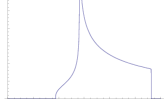
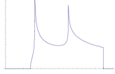
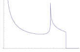
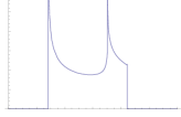
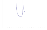
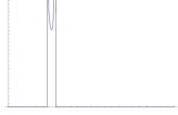
(a) (b) (c) (d) (e) (f)

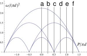
Figure 5: Spectral function of spin $1/2$ Calogero-Sutherland model for $\lambda=1$.

Arikawa pointed out [58] that the hole propagator of SU($2$) Calogero-Sutherland model for $\lambda=1$ is equivalent to the dynamical color correlation function of SU($3$) Haldane-Shastry model[45, 46, 58]. Although the singularities of the upper edge and lower edges have been obtained in earlier works[46, 58], our calculation shows that the spectral function at the middle line diverges with exponent $1/6$, contrary to [46].

7 Conclusion

To calculate the particle propagator of spin Calogero-Sutherland model by Uglov’s method, we transformed the field annihilation operator on Yangian Gelfand-Zetlin basis by the mapping $\Omega$ and proved that it becomes also the field annihilation operator on gl₂-Jack polynomials. This ensures the possibility of calculating 1-particle Green’s function using the Uglov’s method.

Next, with use of this method, we calculated hole propagator for non-negative integer interaction parameter by taking the restricted product over Young diagrams of intermediate states. Thermodynamic limit of hole propagator was also taken, and we confirmed that the result obtained here coincides with that of the former results with Jack polynomial with prescribed symmetry. Spectral function for $\lambda=1$ was calculated, and drawn in energy-momentum plane. There appear the divergences of intensity on one and two quasi-hole excitation lines.

The calculation of particle propagator will be published in a separate paper.

Appendix A Restriction on the Product

The number of the squares of the subset of the Young diagram, $|C_{2}(\mu)|$ and $|H_{2}(\mu)|$, can be uniquely described in terms of $n$, the number of the columns which belong to $Q$. This can be verified by describing $|C_{2}(\mu)|-|D(\mu)\setminus C_{2}(\mu)|$ and $|H_{2}(\mu)|-|D(\mu)\setminus H_{2}(\mu)|$ in terms of $n$, where $A\setminus B$ means the complement of $B$ in $A$.

In each column and each row of the Young diagram, the element of $C_{2}(\mu)$ and that of $D(\mu)\setminus C_{2}(\mu)$ are aligned alternately, and at the upper left of the diagram $s=(1,1)\in C_{2}(\mu)$. From the definition of the set $P$ and $Q$ ((84) and (85)), $j$-th column with $j\in P$ has even number of squares for odd $j$ and odd number for even $j$. Thus the square at the bottom of the $j$-th column in $P$ is an element of $D(\mu)\setminus C_{2}(\mu)$. For $n=0$, all the columns belong to the set $P$, and therefore $|C_{2}(\mu)|-|D(\mu)\setminus C_{2}(\mu)|=-\lambda$. The change of a column in $P$ to $Q$ increases $|C_{2}(\mu)-D(\mu)/C_{2}(\mu)|$ by one (Figure 6). We thus obtain

$$|C_{2}(\mu)|-|D(\mu)\setminus C_{2}(\mu)|=-\lambda+n.$$ (108)

Figure 6: The relation between the number of the squares of $C_{2}(\mu)$ and $D(\mu)\setminus C_{2}(\mu)$ and $n$. White squares are the elements of $C_{2}(\mu)$, and shaded squares are that of $D(\mu)\setminus C_{2}(\mu)$. For $n=0$, the bottom of each column are shaded squares (the elements of the $D(\mu)\setminus C_{2}(\mu)$), and for $n>0$, there appears the white square (the elements of the $C_{2}(\mu)$) in $n$ columns.

Next we describe $|H_{2}(\mu)|-|D(\mu)\setminus H_{2}(\mu)|$ in terms of $n$. First we consider a partition having no adjacent columns with the same length, and then we consider the general case. In each column, the square at the bottom $s=(\mu_{j}^{\prime},j)$ is an element of $D(\mu)\setminus H_{2}(\mu)$. The element of $H_{2}(\mu)$ and that of $D(\mu)\setminus H_{2}(\mu)$ are aligned alternately except for several rows. The exceptions occur at the $\mu_{k}^{\prime}$-th row and $\mu_{k}^{\prime}+1$-th row in $j$-th column with $k=[j+1,j+2,\cdots,2\lambda+1]$, where two elements of the same subset $H_{2}(\mu)$ or $D(\mu)\setminus H_{2}(\mu)$ are aligned vertically (Figure 7). Thus we remove the $\mu_{j}^{\prime}+1$-th row with $j=[2,3,\cdots,2\lambda+1]$ from the original Young diagram, and make the diagrams $D(\tilde{\mu})$ in which the element of $H_{2}(\mu)$ and that of $D(\mu)\setminus H_{2}(\mu)$ are aligned alternately without any exceptions in each column. The removed $2\lambda$ rows make a new diagram $D(\Delta\mu)$ with length $2\lambda$ and $(\Delta\mu)_{1}=2\lambda$ (Figure 7).

For $n=0$, each column of $D(\tilde{\mu})$ has even number of squares. Therefore, the contribution to $|H_{2}(\mu)|-|D(\mu)\setminus H_{2}(\mu)|$ from $\tilde{\mu}$ is given by

$$|H_{2}(\mu)|_{\tilde{\mu}}-|D(\mu)\setminus H_{2}(\mu)|_{\tilde{\mu}}=0.$$ (109)

When a column in $D(\mu)$ changes from $P$ to $Q$, the number of columns in $D(\tilde{\mu})$ with odd length increases by one. We thus obtain

$$|H_{2}(\mu)|_{\tilde{\mu}}-|D(\mu)\setminus H_{2}(\mu)|_{\tilde{\mu}}=-n$$ (110)

for $n\geq 0$.

Now we consider the contribution of $D(\Delta\mu)$ to $|H_{2}(\mu)|-|D(\mu)\setminus H_{2}(\mu)|$. The square $s=(j,k)$ with $1\leq j\leq 2\lambda\,,\,$ $1\leq k\leq 2\lambda+1-j$ in $D(\Delta\mu)$ comes from $s^{\prime}=(\mu^{\prime}_{2\lambda+2-j}+1,k)$ in $D(\mu)$. With use of $a(s^{\prime})=2\lambda+2-j-k-1$ and $l(s^{\prime})=\mu^{\prime}_{k}-\mu^{\prime}_{2\lambda+2-j}-1$, it follows that

$$a(s^{\prime})+l(s^{\prime})+1\equiv\left\{\begin{array}[]{cc}1&(k,2\lambda+2-j)\in(P,P)\mbox{ or }(Q,Q)\\ 0&(k,2\lambda+2-j)\in(P,Q)\mbox{ or }(Q,P)\\ \end{array}\right.,$$ (111)

and hence $s=(j,k)\in H_{2}(\mu)$ in $D(\Delta\mu)$ $\Leftrightarrow$ $(k,2\lambda+2-j)\in(P,Q)\mbox{ or }(Q,P)$. Since two coordinates $k$ and $2\lambda+2-j$ vary with $1\leq k<2\lambda+2-j\leq 2\lambda+1$,

$$|H_{2}(\mu)|_{\Delta\mu}=n(2\lambda+1-n)$$ (112)

$$|D(\mu)\setminus H_{2}(\mu)|_{\Delta\mu}=n(n-1)/2+(2\lambda+1-n)(2\lambda-n)/2$$ (113)

and

$$|H_{2}(\mu)|_{\Delta\mu}-|D(\mu)\setminus H_{2}(\mu)|_{\Delta\mu}=-2n^{2}+2(2\lambda+1)n-\lambda(2\lambda+1)$$ (114)

holds. From (110) and (114), we obtain

$$|H_{2}(\mu)|-|D(\mu)\setminus H_{2}(\mu)|=-2n^{2}+(4\lambda+1)n-\lambda(2\lambda+1).$$ (115)

Figure 7: Young diagram $D(\mu)$ is decomposed to two diagrams $D(\Delta\mu)$ and $D(\tilde{\mu})$. White squares are the elements of $H_{2}(\mu)$, and shaded squares are that of $D(\mu)\setminus H_{2}(\mu)$. In each column of $D(\Delta\mu)$, the element of $H_{2}(\mu)$ and that of $D(\mu)\setminus H_{2}(\mu)$ are aligned alternately.

Next, we apply the result to a partition having two or more columns with the same length. When a partition have $m$ columns with same length, we extract the $2[m/2]$ neighboring columns from the original partition, where $[n]$ means the maximum integer that does not exceed $n$. Since the extracted $2[m/2]$ columns have the same number of the elements of $H_{2}(\mu)$ and $D(\mu)\setminus H_{2}(\mu)$, there is no contribution to $|H_{2}(\mu)|-|D(\mu)\setminus H_{2}(\mu)|$. We can use the result (115) for the left partition with $2\lambda+1-2[m/2]$ columns and obtain the equation by replacing $\lambda$ in (115) by $\lambda-[m/2]$. The above discussion can be applied to a partition that has more than one set of columns with the same length. These applications, however, do not change the result on the condition $|C_{2}(\mu)|+|H_{2}(\mu)|=|\mu|$.

Appendix B Energy Spectrum and Matrix Elements

In this appendix, we derive (96) and (97) in B.1 and (98), (98) and (100) in B.2.

B.1 Energy spectrum

In the excitation energy $\omega_{\kappa}$ in (65), the energy

$$E_{N-1}(\kappa)=(2\pi/L)^{2}\sum_{i=1}^{N-1}\left(\kappa_{i}+\lambda(N-2i)/2\right)^{2}$$

of $N-1$ particle state $\kappa$ is rewritten as

$$E_{N-1}(\kappa)=(\pi/L)^{2}\sum_{i=1}^{N-1}\left(-\mu_{i}+\lambda+(1+2\lambda)\left(i-N/2\right)+\alpha_{N-i}-1\right)^{2},$$ (116)

with use of

$$\nu_{i}=\alpha_{N-i}-2\kappa_{N-i}-N+1+i$$ (117)

(which is (37) with replacement of $N$ by $N-1$) and

$$\mu=\nu+N/2+\lambda-2$$ (118)

coming from (4.1). In (116), the value of $\alpha_{N-i}$ is given by

$$\alpha_{N-i}=\left\{\begin{array}[]{cc}2,&(i,\mu_{i})\in C_{2}(\mu)\\ 1,&(i,\mu_{i})\in D(\mu)/C_{2}(\mu)\\ \end{array}\right.,$$ (119)

which follows from

$$\alpha_{N-i} =\mu_{i}-i+\underbrace{2\kappa_{N-i}}_{\rm even}+\underbrace{N/2+1-\lambda}_{\rm even}$$ (120)

$$\equiv a^{\prime}(i,\mu_{i})+l^{\prime}(i,\mu_{i})\quad\mbox{mod }2.$$

For $i\in[\mu^{\prime}_{1}+1,N-1]$, we regard $(i,0)$ as an element of $C_{2}(\mu)$ ($D(\mu)\setminus C_{2}(\mu)$) when $i$ is even (odd). With use of (119), $E_{N-1}(\kappa)$ is rewritten as

$$E_{N-1}(\kappa)=\frac{\pi^{2}(1+2\lambda)^{2}}{L^{2}}\left({\cal E}^{\prime}_{N-1}(\kappa)+{\cal E}^{\prime\prime}_{N-1}(\kappa)\right),$$ (121)

with

$${\cal E}^{\prime}_{N-1}(\kappa)=\sum_{i\in[1,N-1];\mbox{\scriptsize\, s.t. }(i,\mu_{i})\in C_{2}(\mu)}\left(i-\frac{N}{2}+\frac{\lambda-\mu_{i}+1}{2\lambda+1}\right)^{2}$$ (122)

and

$${\cal E}^{\prime\prime}_{N-1}(\kappa)=\sum_{i\in[1,N-1];\mbox{\scriptsize\, s.t. }(i,\mu_{i})\in D(\mu)\setminus C_{2}(\mu)}\left(i-\frac{N}{2}+\frac{\lambda-\mu_{i}}{2\lambda+1}\right)^{2}.$$ (123)

Now we consider ${\cal E}^{\prime}_{N-1}(\kappa)$. It is convenient to decompose the sum with respect to $i$ as

$$\sum_{i\in[1,N-1],\atop\mbox{\scriptsize\, s.t. }(i,\mu_{i})\in C_{2}(\mu)}\rightarrow\sum_{j=0}^{2\lambda+1}\sum_{i\in[1+\mu^{\prime}_{j+1},\mu^{\prime}_{j}],\atop\mbox{\scriptsize\, s.t. }(i,\mu_{i})\in C_{2}(\mu)}$$ (124)

In the interval $i\in[1+\mu^{\prime}_{j+1},\mu^{\prime}_{j}]$, $i$’s satisfying $(i,\mu_{i})\in C_{2}(\mu)$ align alternately. The minimum (maximum) value $i^{\square}_{\rm min}(j)$ ($i^{\square}_{\rm max}(j)$) of $i$ in $[1+\mu_{j+1},\mu_{j}]$ satisfying $(i,\mu_{i})\in C_{2}(\mu)$ are given, respectively, by

$$i^{\square}_{\rm min}(j)=\mu^{\prime}_{j+1}+\sigma_{j+1}+3/2,\quad i^{\square}_{\rm max}(j)=\mu^{\prime}_{j}-\sigma_{j}-1/2,$$ (125)

as shown below. First we note that $(i,\mu_{i})=(i,j)$ in the interval $i\in[1+\mu^{\prime}_{j+1},\mu^{\prime}_{j}]$. When $j+1\in Q$, $\mu^{\prime}_{j+1}-(j+1)$ is even and hence $(1+\mu^{\prime}_{j+1},j)\in C_{2}(\mu)$ and $i^{\square}_{\rm min}(j)=1+\mu^{\prime}_{j+1}$. When $j+1\in P$, on the other hand, $\mu^{\prime}_{j+1}-(j+1)$ is odd and hence $(1+\mu^{\prime}_{j+1},j)\in D(\mu)\setminus C_{2}(\mu)$ and $i^{\square}_{\rm min}(j)=2+\mu^{\prime}_{j+1}$. Thus we arrive at the first equation of (125). We can obtain the second equation of (125) in a similar way. In term of $i^{\square}_{\rm min}(j)$ and $i^{\square}_{\rm max}(j)$, ${\cal E}^{\prime}_{N-1}(\kappa)$ is written as

$${\cal E}^{\prime}_{N-1}(\kappa) =\sum_{j=0}^{2\lambda+1}\sum_{i=i^{\square}_{\rm min}(j),i^{\square}_{\rm min}(j)+2,\cdots}^{i^{\square}_{\rm max}(j)}\left(i-\frac{N}{2}+\frac{\lambda-j+1}{2\lambda+1}\right)^{2}$$ (126)

$$=\frac{1}{6}\sum_{j=0}^{2\lambda+1}\left(i^{\square}_{\rm max}(j)+1-N/2+\frac{\lambda-j+1}{2\lambda+1}\right)^{3}$$

$$\quad-\frac{1}{6}\sum_{j=0}^{2\lambda+1}\left(i^{\square}_{\rm min}(j)-1-N/2+\frac{\lambda-j+1}{2\lambda+1}\right)^{3}$$

$$\quad+\frac{1}{6}\sum_{j=0}^{2\lambda+1}\left(-i^{\square}_{\rm max}(j)+i^{\square}_{\rm min}(j)-2\right).$$

In the second equality, we have used following formula:

$$\sum_{i=m,m+2,m+4,\cdots,n}(i+A)^{2}$$

$$=\frac{1}{6}\left[(n+1+A)^{3}-(m-1+A)^{3}-n+m-2\right]$$ (127)

for $n$, $m$ satisfying $n-m$ being a positive and even integer. The expression (126) can be further rewritten as

$${\cal E}^{\prime}_{N-1}(\kappa) =\frac{1}{6}\sum_{j=1}^{2\lambda+1}\left[\left(\tilde{\mu}^{\prime}_{j}-\sigma_{j}\right)^{3}-\left(\tilde{\mu}^{\prime}_{j}+\sigma_{j}+1/(2\lambda+1)\right)^{3}+2\sigma_{j}\right]$$ (128)

$$+\frac{M(M^{2}-1)}{3}+\frac{\lambda^{2}M}{(2\lambda+1)^{2}}+\frac{1}{6}$$

with use of (125) and (95). We can rewrite the expression (123) for ${\cal E}^{\prime\prime}_{N-1}(\kappa)$ in a similar way. First (123) is rewritten as

$${\cal E}^{\prime\prime}_{N-1}(\kappa) =\sum_{j=0}^{2\lambda+1}\sum_{i\in[1+\mu^{\prime}_{j+1},\mu^{\prime}_{j}],\atop\mbox{\scriptsize\, s.t. }(i,\mu_{i})\in D(\mu)\setminus C_{2}(\mu)}\left(i-\frac{N}{2}+\frac{\lambda-j}{2\lambda+1}\right)^{2}$$ (129)

$$=\sum_{j=0}^{2\lambda+1}\sum_{i=i^{\blacksquare}_{\rm min}(j),i^{\blacksquare}_{\rm min}(j)+2,\cdots}^{i^{\blacksquare}_{\rm max}(j)}\left(i-\frac{N}{2}+\frac{\lambda-j}{2\lambda+1}\right)^{2},$$

$$=\frac{1}{6}\sum_{j=0}^{2\lambda+1}\left(i^{\blacksquare}_{\rm max}(j)+1-N/2+\frac{\lambda-j}{2\lambda+1}\right)^{3}$$

$$\quad-\frac{1}{6}\sum_{j=0}^{2\lambda+1}\left(i^{\blacksquare}_{\rm min}(j)-1-N/2+\frac{\lambda-j}{2\lambda+1}\right)^{3}$$

$$\quad+\frac{1}{6}\sum_{j=0}^{2\lambda+1}\left(-i^{\blacksquare}_{\rm max}(j)+i^{\blacksquare}_{\rm min}(j)-2\right)$$

where

$$i^{\blacksquare}_{\rm min}(j)=\mu^{\prime}_{j+1}-\sigma_{j+1}+3/2,\quad i^{\blacksquare}_{\rm max}(j)=\mu^{\prime}_{j}+\sigma_{j}-1/2$$ (130)

are, respectively, defined as the minimum and maximum of $i$ satisfying $(i,\mu_{i})\in D(\mu)/C_{2}(\mu)$ in $[1+\mu^{\prime}_{j+1},\mu^{\prime}_{j}]$. In the last equality in (129), we have used (127). Substituting (130) into (129) and using (95), ${\cal E}^{\prime\prime}_{N-1}(\kappa)$ is expressed as

$${\cal E}^{\prime\prime}_{N-1}(\kappa) =\frac{1}{6}\sum_{j=1}^{2\lambda+1}\left[\left(\tilde{\mu}^{\prime}_{j}+\sigma_{j}-1/(2\lambda+1)\right)^{3}-\left(\tilde{\mu}^{\prime}_{j}-\sigma_{j}\right)^{3}-2\sigma_{j}\right]$$ (131)

$$+\frac{M(M^{2}-1)}{3}+\frac{\lambda^{2}M}{(2\lambda+1)^{2}}+\frac{1}{6}.$$

Substituting (128) and (131) into (121), we obtain

$$E_{N-1}(\kappa) =-(2\lambda+1)\sum_{j=1}^{2\lambda+1}\left(\frac{\pi(\tilde{\mu}^{\prime}_{j}+\sigma_{j})}{L}\right)^{2}+\frac{4\pi^{2}\lambda(\lambda+1)}{3L^{2}}$$ (132)

$$\quad+\underbrace{\frac{2\pi^{2}(2\lambda+1)^{2}M(M^{2}-1)}{3L^{2}}+\frac{2\pi^{2}\lambda^{2}M}{L^{2}}}_{=E_{N}({\rm g})}$$

from which and (65), the expressions (96) and (97) follow.

B.2 Matrix elements

Here we describe $X_{\mu},Y_{\mu}(r),Z_{\mu}(r)$ in the matrix elements in terms of the renormalized momenta (95) and the spin variables (93) and (94). First we consider $X_{\mu}$. The product with respect to $s=(i,j)\in D(\mu)\setminus C_{2}(\mu)$ is taken within each column, and then taken over the column. In the $j$-th column, this condition is equivalent to even (odd) $i$ when $j$ is odd (even). The square $s=(\mu^{\prime}_{j},j)$ belongs to $D(\mu)\setminus C_{2}(\mu)$ when $j\in P$ and $s=(\mu^{\prime}_{j}-1,j)$ belongs to $D(\mu)\setminus C_{2}(\mu)$ when $j\in Q$. The maximum value of $i$ in the $j$-th column is thus expressed as

$$i_{\rm max}=\mu^{\prime}_{j}-\delta_{\sigma_{j}\sigma_{2\lambda+2}}.$$ (133)

The contribution to $X_{\mu}$ from $j$-th column is then given by

$$\prod_{i:{\rm even}}^{i_{\rm max}}\left(-\alpha(j-1)+i/2\right) =\prod_{i^{\prime}=1}^{i_{\rm max}/2}(i^{\prime}-\alpha(j-1))$$ (134)

$$=\frac{\Gamma[i_{\rm max}/2+1-\alpha(j-1)]}{\Gamma[1-\alpha(j-1)]}$$

for odd $j$ and

$$\prod_{i:{\rm odd}}^{i_{\rm max}}\left(-\alpha(j-1)+i/2\right) =\prod_{i^{\prime}=1}^{(i_{\rm max}+1)/2}(i^{\prime}-1/2-\alpha(j-1))$$ (135)

$$=\frac{\Gamma[i_{\rm max}/2+1-\alpha(j-1)]}{\Gamma[1/2-\alpha(j-1)]}$$

for even $j$. We introduce a dummy index $i^{\prime}=i/2$ in (134) and $i^{\prime}=(i+1)/2$ in (135), respectively. From (134) and (135) and with use of

$$\prod_{j\in[1,3,\cdots,2\lambda+1]}\Gamma[1-\alpha(j-1)]\prod_{j\in[2,4,\cdots,2\lambda]}\Gamma[1/2-\alpha(j-1)]$$

$$=\prod_{j=1}^{2\lambda+1}\Gamma[j/(2\lambda+1)],$$ (136)

we obtain

$$X_{\mu}=\prod_{j=1}^{2\lambda+1}\frac{\Gamma[i_{\rm max}/2+1-\alpha(j-1)]}{\Gamma[j/(2\lambda+1)]}.$$ (137)

With use of (133) and (95), (137) becomes (98).

Similarly, we can write $Y_{\mu}(r)$ in terms of $\tilde{\mu}^{\prime}_{j}$ and $\sigma_{j}$ for $j\in[0,2\lambda+1]$, as shown below. When $(i,j)\in C_{2}(\mu)$, both $i$ and $j$ are odd or even. The maximum value $i_{\rm max}$ of $i$ in $j$-th column is given by $i_{\rm max}=\mu^{\prime}_{j}-\delta_{\sigma_{j}\sigma_{0}}$. The contribution to $Y_{\mu}(r)$ from $j$-th column is given by

$$\prod_{i:{\rm odd}}^{i_{\rm max}}(\alpha(j-1)+r+(N-i)/2) =\prod_{i^{\prime}=1}^{(i_{\rm max}+1)/2}(\alpha(j-1)+r+(N+1)/2-i^{\prime})$$ (138)

$$=\frac{\Gamma[\alpha(j-1)+r+(N+1)/2]}{\Gamma[\alpha(j-1)+r+(N-i_{\rm max})/2]}$$

for odd $j$ and

$$\prod_{i:{\rm even}}^{i_{\rm max}}(\alpha(j-1)+r+(N-i)/2) =\prod_{i^{\prime}=1}^{i_{\rm max}/2}(\alpha(j-1)+r+N/2-i^{\prime})$$ (139)

$$=\frac{\Gamma[\alpha(j-1)+r+N/2]}{\Gamma[\alpha(j-1)+r+(N-i_{\rm max})/2]}$$

for even $j$. With use of (95) and the relation

$$\prod_{j\in[1,3,\cdots,2\lambda+1]}\Gamma[\alpha(j-1)+r+(N+1)/2]\prod_{j\in[2,4,\cdots,2\lambda]}\Gamma[\alpha(j-1)+r+N/2]$$

$$=\prod_{j=1}^{2\lambda+1}\Gamma[\alpha+r+N/2+(j-1)/(2\lambda+1)],$$ (140)

the expression $Y_{\mu}(r)$ is obtained as (99).

Next we consider the expression for $Z_{\mu}(r)$ in terms of $\{\tilde{\mu}^{\prime}_{j},\sigma_{j}\}$. It is convenient to decompose $D(\mu)$ as shown in Figure 8.

Figure 8: Young diagram of a quasi-hole state for $\lambda=1$ is decomposed into $D_{jk}$ for calculation of $Z_{\mu}(r)$.

Correspondingly, $Z_{\mu}(r)$ is rewritten as

$$Z_{\mu}(r)=\prod_{j=1}^{2\lambda+1}\prod_{k=j}^{2\lambda+1}\prod_{s\in H_{2}(\mu)\cap D_{jk}}\left(\alpha a(s)+r+l(s)/2\right)$$ (141)

with

$$D_{jk}=\left\{s=(i,j)|i\in[1+\mu^{\prime}_{k+1},\mu^{\prime}_{k}]\right\}.$$ (142)

Within $D_{jk}$, the arm length $a(s)$ is constant ($=k-j$) and hence the squares which belong to $H_{2}(\mu)$ and $D(\mu)\setminus H_{2}(\mu)$ are, respectively, aligned alternately. Let $i_{\rm min}$ and $i_{\rm max}$ be, respectively, the minimum and maximum values of $i$ in $s\in H_{2}(\mu)\cap D_{jk}$. Thus the product over $s=(i,j)\in H_{2}(\mu)\cap D_{jk}$ is expressed as the product over $i^{\prime}=0,1,\cdots,(i_{\rm max}-i_{\rm min})/2$ with $i=2i^{\prime}+i_{\rm min}$. The contribution to $Z_{\mu}(r)$ from $D_{jk}$ is given by

$$\prod_{s\in H_{2}(\mu)\cap D_{jk}}\left(\alpha a(s)+r+l(s)/2\right)$$

$$=\sum_{i^{\prime}=0}^{(i_{\rm max}-i_{\rm min})/2}(\alpha(k-j)+r+\mu^{\prime}_{j}/2-i_{\rm min}/2-i^{\prime})$$

$$=\frac{\Gamma[\alpha(k-j)+r+\mu^{\prime}_{j}/2-i_{\rm min}/2+1]}{\Gamma[\alpha(k-j)+r+\mu^{\prime}_{j}/2-i_{\rm max}/2]}.$$ (143)

The maximum value $i_{\rm max}$ of $i$ in $H_{2}(\mu)\cap D_{jk}$ is expressed as

$$i_{\rm max}=\mu^{\prime}_{k}-\delta_{\sigma_{j}\sigma_{k}}$$ (144)

as shown below.

For $s\in D_{jk}$, $a(s)$ is $k-j$ and $l(s)=\mu^{\prime}_{j}-i$ and hence $h(s)=a(s)+l(s)+1$ is written as

$$h(s)=\mu^{\prime}_{j}-j+k-i+1=\mu^{\prime}_{j}-j-(\mu^{\prime}_{k}-k)+\mu^{\prime}_{k}-i+1.$$ (145)

When $(j,k)\in(P,P)$ or $(Q,Q)$, both $\mu^{\prime}_{j}-j$ and $\mu^{\prime}_{k}-k$ are odd or even and hence for $(i,j)\in H_{2}(\mu)\cap D_{jk}$,

$$\mu^{\prime}_{k}-1\equiv i\quad{\rm mod}\,2.$$ (146)

When $(j,k)\in(P,Q)$ or $(Q,P)$, on the other hand, the sum of $\mu^{\prime}_{j}-j$ and $\mu^{\prime}_{k}-k$ is odd and hence,

$$\mu^{\prime}_{k}\equiv i\quad{\rm mod}\,2.$$ (147)

The two relations (146) and (147) are expressed as (144) in a unified way. In a similar way, $i_{\rm min}$ is expressed as

$$i_{\rm min}=\mu^{\prime}_{k+1}+1+\delta_{\sigma_{j}\sigma_{k+1}}$$ (148)

respectively.

The expression (143) is further written as

$$\prod_{s\in H_{2}(\mu)\cap D_{jk}}\left(\alpha a(s)+r+l(s)/2\right)$$

$$=\frac{\Gamma[(\tilde{\mu}^{\prime}_{j}-\tilde{\mu}^{\prime}_{k+1}-\delta_{\sigma_{j}\sigma_{k+1}})/2+r-\alpha+1/2]}{\Gamma[(\tilde{\mu}^{\prime}_{j}-\tilde{\mu}^{\prime}_{k}+\delta_{\sigma_{j}\sigma_{k}})/2+r]},$$ (149)

with use of (144), (148) and (95). From (149), the expression (100) for $Z_{\mu}(r)$ follows.

Appendix C Spectral Weight

The triple integral in the spectral function for $\lambda=1$,

$$A^{-}(\epsilon,p) =C\int_{-1}^{1}\rmd u_{1}\int_{-1}^{1}\rmd u_{2}\int_{-1}^{1}\rmd u_{3}\,\,\delta\left(p-\frac{\pi d}{2}(u_{1}+u_{2}+u_{3})\right)$$ (150)

$$\,\,\,\quad\times\delta\!\left(\epsilon-\frac{3(\pi d)^{2}}{4}\left(3-u_{1}^{2}-u_{2}^{2}-u_{3}^{2}\right)\right)F(u_{1},u_{2},u_{3})$$

with

$$F(u_{1},u_{2},u_{3})$$

$$=\left|u_{2}-u_{3}\right|^{4/3}\left|u_{1}-u_{3}\right|^{-2/3}\left|u_{1}-u_{2}\right|^{-2/3}\prod_{j=1}^{3}\left(1-u_{j}^{2}\right)^{-1/3}$$ (151)

reduces to an integral on a curve determined by the sphere, plane, and the cube

$$\epsilon=\frac{3(\pi d)^{2}}{4}\left(3-u_{1}^{2}-u_{2}^{2}-u_{3}^{2}\right)$$ (152)

$$p=\frac{\pi d}{2}(u_{1}+u_{2}+u_{3})$$ (153)

$$|u_{i}|\leq 1,\quad i=1,2,3.$$ (154)

The cross section between (153) and (154) is triangular when

$$\pi d/2\leq p\leq 3\pi d/2$$ (155)

and hexagon when

$$0\leq p\leq\pi d/2,$$ (156)

as shown in Figure 10.

In the following, we consider the case (155) only. The case (156) can be discussed similarly. The integral in (150) is on a circle when

$$\frac{\pi d}{2}\leq p\leq\frac{3\pi d}{2},\mbox{ and }-\frac{3}{2}\left(p-\frac{\pi d}{2}\right)^{2}+\frac{3}{2}(\pi d)^{2}\leq\epsilon\leq-p^{2}+\frac{9}{4}(\pi d)^{2},$$ (157)

and it is on three disconnected pieces of arc when

$$\pi d/2\leq p\leq 3\pi d/2$$

and

$$-3(p-\pi d)^{2}+\frac{3}{4}(\pi d)^{2}\leq\epsilon\leq-\frac{3}{2}\left(p-\frac{\pi d}{2}\right)^{2}+\frac{3}{2}(\pi d)^{2},$$

as shown by bold curves in Figure 10.

Figure 9: Cross section of the plane (153) and the cube (154). The cross section is triangular PQR when $p\in[\pi d/2,3\pi d/2]$ and hexagon when $p\in[0,\pi d/2]$. Figure 10: Cross section of the plane (153) and the cube (154) for $p\in[\pi d/2,3\pi d/2]$.

The integrand $F(u_{1},u_{2},u_{3})$ in (150) diverges when

$$u_{1}=u_{3},\quad u_{1}=u_{2}\quad\mbox{or }|u_{j}|=1\mbox{ for }j=1,2,3,$$ (158)

which are represented by solid lines in Figure 10. When the contour of the integral passes near the crossing points of the above lines (158), the spectral function becomes singular. Those crossing points are given by

$$(u_{1},u_{2},u_{3})= \left(\frac{2p}{3\pi d}\,,\,\frac{2p}{3\pi d}\,,\,\frac{2p}{3\pi d}\right),$$ (159)

$$\left(1\,,\,1\,,\,-2+\frac{2p}{\pi d}\right),$$ (160)

$$\left(-\frac{1}{2}+\frac{p}{\pi d}\,,\,-\frac{1}{2}+\frac{p}{\pi d}\,,\,1\right)$$ (161)

and their equivalent points. They are depicted in Figure 10 by dots. The singularity of the spectral function near the upper edge $\epsilon=(3\pi d/2)^{2}(1-(2p/(\pi d))^{2})$ of the support comes from (159). The point (160) yields the singularity of $A(\epsilon,p)$ near the lower edge $\epsilon=3(\pi d/2)^{2}(2p/(\pi d)-1)(3-2p/(\pi d)))$. (161) is relevant to the singularity near

$$\epsilon=\frac{3}{2}\left(p+\frac{\pi d}{2}\right)\left(\frac{3\pi d}{2}-p\right)\equiv\epsilon_{p}.$$ (162)

The singularities near the upper edge and lower edge have been obtained in earlier papers[62, 46]. We thus consider the singularity when $\delta\epsilon\equiv\epsilon-\epsilon_{p}\sim 0$ in the following.

Now we introduce the Cartesian coordinate $\mbox{\boldmath$e$}_{i}\cdot\mbox{\boldmath$e$}_{j}=\delta_{ij}$ $i,j=1,2,3$ and define the vector

$$\mbox{\boldmath$u$}=u_{1}\mbox{\boldmath$e$}_{1}+u_{2}\mbox{\boldmath$e$}_{2}+u_{3}\mbox{\boldmath$e$}_{3}.$$ (163)

We define another Cartesian coordinate

$$\mbox{\boldmath$e$}_{\xi}=-\mbox{\boldmath$e$}_{1}/\sqrt{6}-\mbox{\boldmath$e$}_{2}/\sqrt{6}+2\mbox{\boldmath$e$}_{3}/\sqrt{6},$$

$$\mbox{\boldmath$e$}_{\eta}=-\mbox{\boldmath$e$}_{1}/\sqrt{2}+\mbox{\boldmath$e$}_{2}/\sqrt{2},$$

$$\mbox{\boldmath$e$}_{\zeta}=(\mbox{\boldmath$e$}_{1}+\mbox{\boldmath$e$}_{2}+\mbox{\boldmath$e$}_{3})/\sqrt{3}$$ (164)

and circular coordinate on $\mbox{\boldmath$e$}_{\xi}-\mbox{\boldmath$e$}_{\eta}$ plane

$$\mbox{\boldmath$e$}_{\rho}=\mbox{\boldmath$e$}_{\xi}\cos\theta+\mbox{\boldmath$e$}_{\eta}\sin\theta,$$

$$\mbox{\boldmath$e$}_{\theta}=-\mbox{\boldmath$e$}_{\xi}\sin\theta+\mbox{\boldmath$e$}_{\eta}\cos\theta.$$ (165)

Note that $\{\mbox{\boldmath$e$}_{\xi},\mbox{\boldmath$e$}_{\eta},\mbox{\boldmath$e$}_{\zeta}\}$ forms a cylindrical coordinate as shown in Figure 11.

Figure 11: Cartesian coordinate $\{\mbox{\boldmath$e$}_{\xi},\mbox{\boldmath$e$}_{\eta},\mbox{\boldmath$e$}_{\zeta}\}$ and cylindrical coordinate $\{\mbox{\boldmath$e$}_{\rho},\mbox{\boldmath$e$}_{\theta},\mbox{\boldmath$e$}_{\zeta}\}$.

In terms of (164) and (165), we rewrite $u$ as

$$\mbox{\boldmath$u$}=u_{\rho}\mbox{\boldmath$e$}_{\rho}+u_{\zeta}\mbox{\boldmath$e$}_{\zeta}.$$ (166)

In the following, we change the variables of integral in (150) from $(u_{1},u_{2},u_{3})$ to $(u_{\rho},\theta,u_{\zeta})$. From (163)-(166), we obtain

$$u_{1}=\mbox{\boldmath$u$}\cdot\mbox{\boldmath$e$}_{1}=u_{\rho}(-\cos\theta/\sqrt{6}-\sin\theta/\sqrt{2})+u_{\zeta}/\sqrt{3}$$

$$u_{2}=\mbox{\boldmath$u$}\cdot\mbox{\boldmath$e$}_{2}=u_{\rho}(-\cos\theta/\sqrt{6}+\sin\theta/\sqrt{2})+u_{\zeta}/\sqrt{3}$$

$$u_{3}=\mbox{\boldmath$u$}\cdot\mbox{\boldmath$e$}_{3}=2u_{\rho}\cos\theta/\sqrt{6}+u_{\zeta}/\sqrt{3}.$$ (167)

The spectral function (150) is rewritten as

$$A^{-}(\epsilon,p) =C\int\rmd u_{\rho}u_{\rho}\int\rmd\theta\int\rmd u_{\zeta}\,\,\delta\left(p-\frac{\sqrt{3}\pi du_{\zeta}}{2}\right)$$ (168)

$$\,\,\,\quad\times\delta\!\left(\epsilon-3(\pi d/2)^{2}\left(3-u_{\rho}^{2}-u_{\zeta}^{2}\right)\right)$$

$$\,\,\,\quad\times F(u_{1},u_{2},u_{3}).$$

From the delta functions, $u_{\rho}$ and $u_{\zeta}$ are forced to be

$$u_{\rho}=\sqrt{3-4(\epsilon+p^{2})/(3\pi^{2}d^{2})},\quad u_{\zeta}=2p/(\sqrt{3}\pi d),$$ (169)

respectively. As a result, $A^{-}(\epsilon,p)$ becomes

$$A^{-}(\epsilon,p)=\frac{4C}{(\sqrt{3}\pi d)^{3}}\int\rmd\theta F(\bar{u}_{1}(\theta),\bar{u}_{2}(\theta),\bar{u}_{3}(\theta))$$ (170)

with

$$\bar{u}_{1}(\theta)=\sqrt{(1/2-p^{\prime}/3)^{2}-2\delta\epsilon^{\prime}/9}(-\cos\theta-\sqrt{3}\sin\theta)+2p^{\prime}/3$$

$$\bar{u}_{2}(\theta)=\sqrt{(1/2-p^{\prime}/3)^{2}-2\delta\epsilon^{\prime}/9}(-\cos\theta+\sqrt{3}\sin\theta)+2p^{\prime}/3$$

$$\bar{u}_{3}(\theta)=\sqrt{(1-2p^{\prime}/3)^{2}-4\delta\epsilon^{\prime}/9}\cos\theta+2p^{\prime}/3.$$ (171)

Here we have introduced $\delta\epsilon^{\prime}\equiv\delta\epsilon/(\pi d)^{2}$ and $p^{\prime}=p/(\pi d)$. The integral in (170) runs over

$$\theta\in[0,2\pi],\quad\mbox{for}\quad\delta\epsilon>0$$

$$\theta\in[\theta_{0},2\pi/3-\theta_{0}]\cup[2\pi/3+\theta_{0},4\pi/3-\theta_{0}]\cup[4\pi/3+\theta_{0},2\pi-\theta_{0}]$$ (172)

for $\delta\epsilon<0$ with

$$\theta_{0}=\arcsin\left[\sqrt{\frac{-2\delta\epsilon^{\prime}}{(3/2-p^{\prime})^{2}-2\delta\epsilon^{\prime}}}\,\right].$$

The point (161) and equivalent points

$$\left(1\,,\,-\frac{1}{2}+\frac{p}{\pi d}\,,\,-\frac{1}{2}+\frac{p}{\pi d}\right),\quad\left(-\frac{1}{2}+\frac{p}{\pi d}\,,\,1\,,\,-\frac{1}{2}+\frac{p}{\pi d}\right)$$ (173)

correspond to $\delta\epsilon^{\prime}=0$ and $\theta=0,\,2\pi/3,\,4\pi/3$, respectively. The most singular contribution to $A^{-}(\epsilon,p)$ for $\delta\epsilon=0$ comes from the vicinity of $\theta=0$, where the factors $|u_{1}-u_{2}|^{-2/3}(1-u_{3})^{-1/3}$ become singular in $F(u_{1},u_{2},u_{3})$. Therefore, we approximate $F(u_{1},u_{2},u_{3})$ as

$$F \propto(\bar{u}_{1}(\theta)-\bar{u}_{2}(\theta))^{-2/3}(1-\bar{u}_{3}(\theta))^{-1/3}\propto\frac{|\sin\theta|^{-2/3}}{(1-g\cos\theta)^{1/3}}$$ (174)

with $g=\sqrt{1-\delta\epsilon^{\prime}/(p^{\prime}-3/2)^{2}}$. $A^{-}(\epsilon,p)$ is evaluated as

$$A^{-}(\epsilon,p)\propto\int_{0}^{\theta_{\rm c}}\frac{|\sin\theta|^{-2/3}}{(1-g\cos\theta)^{1/3}}\rmd\theta$$ (175)

for $\delta\epsilon>0$ and $\delta\epsilon\sim 0$ and

$$A^{-}(\epsilon,p)\propto\int_{\theta_{0}}^{\theta_{\rm c}}\frac{|\sin\theta|^{-2/3}}{(1-g\cos\theta)^{1/3}}\rmd\theta$$ (176)

for $\delta\epsilon<0$ and $\delta\epsilon\sim 0$. Here $\theta_{\rm c}$ is a cut-off angle of the order unity. We can take $\theta_{\rm c}=\pi/3,$ or $\pi/2$, for example. First we evaluate (175). Introducing $t=\tan(\theta/2)$, $t_{\rm c}=\tan(\theta_{\rm c}/2)$ and $\tilde{g}=(1-g)/(1+g)$, (175) becomes

$$A^{-}(\epsilon,p)\propto\int_{0}^{t_{\rm c}}\frac{t^{-2/3}(1+t^{2})^{-4/3}}{(t^{2}+\tilde{g})^{1/3}}\rmd t.$$ (177)

We rewrite (177) as

$$\int_{0}^{t_{\rm c}}\frac{t^{-2/3}(1+t^{2})^{-4/3}}{(t^{2}+\tilde{g})^{1/3}}\rmd t$$ (178)

$$=\int_{0}^{t_{\rm c}}\frac{t^{-2/3}}{(t^{2}+\tilde{g})^{1/3}}\rmd t+\int_{0}^{t_{\rm c}}\frac{t^{-2/3}((1+t^{2})^{-4/3}-1)}{(t^{2}+\tilde{g})^{1/3}}\rmd t$$ (179)

The second integral of the right-hand side converges when $\tilde{g}=0$. The first term of the right-hand side, on the other hand, is rewritten as

$$\tilde{g}^{-1/6}\int_{0}^{t_{\rm c}\tilde{g}^{-1/2}}\frac{\tau^{-2/3}}{(\tau^{2}+1)^{1/3}}\rmd\tau\sim\tilde{g}^{-1/6}\int_{0}^{\infty}\frac{\tau^{-2/3}}{(\tau^{2}+1)^{1/3}}\rmd\tau.$$ (180)

Since $\tilde{g}\propto\delta\epsilon$, we arrive at

$$A^{-}(\epsilon,p)\propto(\delta\epsilon)^{-1/6}$$ (181)

when $\delta\epsilon>0$ and $\delta\epsilon\sim 0$.

The singularity near $\delta\epsilon=0$ and $\delta\epsilon<0$ is evaluated similarly. Introducing $t_{0}=\tan(\theta_{0}/2)$, (176) becomes

$$A^{-}(\epsilon,p) \propto\int_{t_{0}}^{t_{\rm c}}\frac{t^{-2/3}(1+t^{2})^{-4/3}}{(t^{2}+\tilde{g})^{1/3}}\rmd t\sim\tilde{g}^{-1/6}\int_{t_{0}\tilde{g}^{-1/2}}^{t_{\rm c}\tilde{g}^{-1/2}}\frac{\tau^{-2/3}}{(\tau^{2}+1)^{1/3}}\rmd\tau$$ (182)

When $\tilde{g}\sim 0$, equivalently $\delta\epsilon\sim 0$, $t_{0}\tilde{g}^{-1/2}$ is the order of unity and hence,

$$A^{-}(\epsilon,p)\propto(-\delta\epsilon)^{-1/6}$$ (183)

when $\delta\epsilon<0$ and $\delta\epsilon\sim 0$.

References

References

- [1] Calogero F 1969 J. Math. Phys. 10 2191
- [2] Calogero F 1969 J. Math. Phys. 10 2197
- [3] Sutherland B 1971 J. Math. Phys. 12 246
- [4] Sutherland B 1971 J. Math. Phys. 12 251
- [5] Sutherland B 1971 Phys. Rev. A 4 2019
- [6] Sutherland B 1972 Phys. Rev. A 5 1372
- [7] Olshanetsky M A and Perelomov A M 1983 Phys. Rep. 94 313
- [8] Sutherland B 2004 Beautiful models (Singapore, World Scientific)
- [9] Shiraishi J 2003 Lectures on Quantum Integrable Systems (in Japanese), (Tokyo, Saiensu-sha)
- [10] Haldane F D M 1991 Phys. Rev. Lett.67 937
- [11] Wu Y-S 1994 Phys. Rev. Lett.73 922
- [12] Wu Y-S 1995 Phys. Rev. Lett.74 3906 (errata)
- [13] Stanley R P 1989 Adv. in Math. 77 76
- [14] Macdonald I G 1995 Symmetric functions and Hall polynomials 2nd ed., (Oxford, Oxford University Press)
- [15] Kawakami N and Yang S-K 1991 Phys. Rev. Lett. 67 2493
- [16] Awata H, Matsuo Y, Odake S and Shiraishi J 1995 Phys. Lett. B 347 49
- [17] Abanov A G and Wiegmann P B 2005 Phys. Rev. Lett. 95 076402
- [18] Simon B D, Lee P A and Altshuler B L 1993 Phys. Rev. Lett. 70 4122
- [19] Minahan J A and Polychronakos 1994 A P Phys. Rev.B 50 4236-4239
- [20] Forrester P J 1995 J. Math. Phys. 36 86
- [21] Haldane F D M and Zirnbauer M R 1993 Phys. Rev. Lett. 71 4055
- [22] Ha Z N C 1994 Phys. Rev. Lett. 73 1574
- [23] Ha Z N C 1995 Phys. Rev. Lett. 74 620 (errata)
- [24] Lesage F, Pasquier V and Serban D 1995 Nucl. Phys. B 435 585
- [25] Ha Z N C 1995 Nucl. Phys. B 435 604
- [26] Zirnbauer M R and Haldane F D M 1995 Phys. Rev.B 52 8729
- [27] Serban D, Lesage F and Pasquier V 1996 Nucl. Phys. B 466 499
- [28] Korepin V E, Bogoliubov N M and Izergin A G 1993 Quantum inverse scattering method and correlation functions (Cambridge University Press, Cambridge)
- [29] Mucciolo E R, Shastry B S, Simons B D and Altshuler B L 1994 Phys. Rev. B 49 15197
- [30] Pustilnik M 2006 Phys. Rev. Lett. 97 036404
- [31] Ha Z N C and Haldane F D M 1992 Phys. Rev. B 46 9359
- [32] Kawakami N 1992 Phys. Rev. B 46 1005
- [33] Minahan J A and Polychronakos A P 1993 Phys. Lett. B 302 265
- [34] Drinfel’d V G 1985 Sov. Math. Dokl. 32 254
- [35] Bernard D, Gaudin M, Haldane F D M and Pasquier V 1993 J. Phys. A: Math. Gen.26 5219
- [36] Haldane F D M 1988 Phys. Rev. Lett.60 635
- [37] Shastry B S Phys. Rev. Lett.60 639
- [38] Polychronakos A P 1993 Phys. Rev. Lett.70 2329
- [39] Sutherland B and Shastry B S 1993 Phys. Rev. Lett.71 5
- [40] Kawakami N 1993 J. Phys. Soc. Japan62 2270
- [41] Kato Y 1997 Phys. Rev. Lett.78 3193
- [42] Kato Y and Yamamoto T 1998 J. Phys. A: Math. Gen.31 9171
- [43] Uglov D 1998 Commun. Math. Phys. 191 663
- [44] Yamamoto T and Arikawa M 1999 J. Phys. A: Math. Gen.32 3341
- [45] Yamamoto T, Saiga Y, Arikawa M and Kuramoto Y 2000 Phys. Rev. Lett.84 1308
- [46] Yamamoto T, Saiga Y, Arikawa M and Kuramoto Y 2000 J. Phys. Soc. Japan69 900
- [47] Baker T H and Forrester P J 1997 Nucl. Phys.B 492 682
- [48] Dunkl C F 1998 Commun. Math. Phys. 197 451
- [49] Opdam E 1995 Acta. Math. 175 75
- [50] Sahi S 1996 IMRN 20 997
- [51] Dunkl C F 1989 Trans. AMS 311 167
- [52] Cherednik I V 1991 Inv. Math. 106 411
- [53] Nazarov M and Tarasov V 1998 J. Reine Angew. Math. 496 181
- [54] Takemura K and Uglov D 1997 J. Phys. A: Math. Gen.30 3685
- [55] Kuramoto Y and Kato Y unpublished
- [56] Arikawa M and Saiga Y 2006 J. Phys. A: Math. Gen.39 10603
- [57] Kiwata H and Akutsu Y 1992 J. Phys. Soc. Japan61 2161
- [58] Arikawa M unpublished
- [59] Ruijsenaars S N M and Schneider H 1986 Ann. Phys. 170 370
- [60] Ruijsenaars S N M 1987 Comm. Math. Phys. 110 191
- [61] Konno H 1996 Nucl. Phys.B 473 579
- [62] Kato Y, Yamamoto T and Arikawa M 1997 J. Phys. Soc. Japan66 1954