Edge Effect on Electronic Transport Properties of Graphene Nanoribbons and Presence of Perfectly Conducting Channel

Abstract

Numerical calculations have been performed to elucidate unconventional electronic transport properties in disordered nanographene ribbons with zigzag edges (zigzag ribbons). The energy band structure of zigzag ribbons has two valleys that are well separated in momentum space, related to the two Dirac points of the graphene spectrum. The partial flat bands due to edge states make the imbalance between left- and right-going modes in each valley, i.e. appearance of a single chiral mode. This feature gives rise to a perfectly conducting channel in the disordered system, i.e. the average of conductance $\langle g\rangle$ converges exponentially to 1 conductance quantum per spin with increasing system length, provided impurity scattering does not connect the two valleys, as is the case for long-range impurity potentials. Ribbons with short-range impurity potentials, however, through inter-valley scattering, display ordinary localization behavior. Symmetry considerations lead to the classification of disordered zigzag ribbons into the unitary class for long-range impurities, and the orthogonal class for short-range impurities. The electronic states of graphene nanoribbons with general edge structures are also discussed, and it is demonstrated that chiral channels due to the edge states are realized even in more general edge structures except for armchair edges.

I Introduction

Graphene being for many decades only a domain to theoretical studies, has recently been fabricated with ingenious methods and has initiated intensive and diverse research on this system.novoselov The honeycomb crystal structure of single layer graphene consists of two inequivalent sublattices and results in a unique band structure for the itinerant $\pi$-electrons near the Fermi energy which behave as massless Dirac fermion. The valence and conduction bands touch conically at two nonequivalent Dirac points, called $\bm{K_{+}}$ and $\bm{K_{-}}$ point, which form a time-reversed pair, i.e. opposite chirality.geim The chirality and a Berry phase of $\pi$ at the two Dirac points provide an environment for highly unconventional and fascinating two-dimensional electronic properties, such as the half-integer quantum Hall effect,qhe1 ; qhe2 the absence of backward scattering,ando.nakanishi $\pi$-phase shift of the Shubnikov-de Haas oscillations.kopelvich

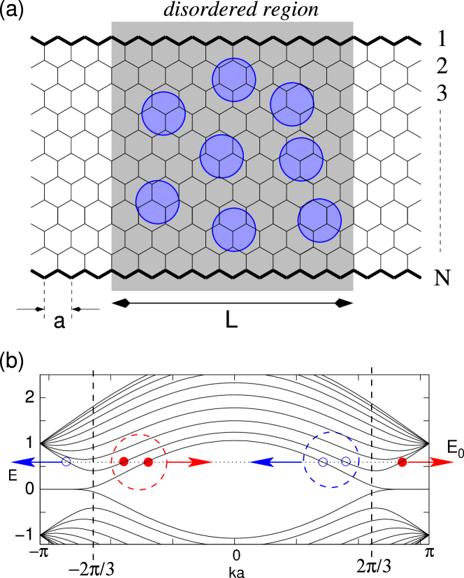
Figure 1: (a) Structure of graphene zigzag ribbon. The disordered region with randomly distributed impurities lies in the shaded region and has the length $L$. The lattice constant is $a$ and the ribbon width $N$ is defined as the number of the zigzag chains. Randomly distributed blue circles schematically represent the long ranged impurities. (b) Energy dispersion of zigzag ribbon with $N=10$. The valleys in the energy dispersion near $k=2\pi/3a$ ($k=-2\pi/3a$) originate from the Dirac $\bm{K_{+}}$($\bm{K_{-}}$)-point of graphene. The red-filled (blue-unfilled) circles denote the right (left)-moving open channel at the energy $E_{0}$(dashed horizontal line). In the left(right) valley, the degeneracy between right and left moving channels is missing due to one excess right(left)-going mode. The time-reversal symmetry under the intra-valley scattering is also broken.

The successive miniaturization of the graphene electronic devices inevitably demands the clarification of edge effects on the electronic structures and electronic transport properties of nanometer-sized graphenes. The presence of edges in graphene has strong implications for the low-energy spectrum of the $\pi$-electrons.peculiar ; prb.1999 There are two basic shapes of edges, armchair and zigzag which determine the properties of graphene ribbons. It was shown that ribbons with zigzag edges (zigzag ribbon) possess localized edge states with energies close to the Fermi level.peculiar ; prb.1999 ; Phd These edge states correspond to the non-bonding configurations as can be seen by examining the analytic solution for semi-infinite graphite with a zigzag edge for which the wave functions of the edge states reside on one sublattice only.peculiar In contrast, edge states are completely absent for ribbons with armchair edges. Recent experiments support the evidence of edge localized states.enoki ; fukuyama Also, graphene nanoribbons can experimentally be produced by using lithography techniques.Kim

The electronic transport through zigzag ribbons shows a number of intriguing phenomena such as zero-conductance Fano resonances,prl ; prb vacancy configuration dependent transport,vacancy valley filtering,rycerz , half-metallic conductionson and spin Hall effect.kane It is also expected that the edge states play an important role for the magnetic properties in nanometer-sized graphite systems, because of their relatively large contribution to the density of states at the Fermi energy.peculiar ; prb.1999 ; kusakabe ; sokada ; harigaya ; takai ; palacios

Since the graphene nanoribbons can be viewed as a new class of the quantum wires, one might expect that random impurities inevitably cause the Anderson localization, i.e. conductance decays exponentially with increasing system length $L$ and eventually vanishes in the limit of $L\to\infty$. However, it was shown that carbon nanotubes with long-ranged impurities possess a perfectly conducting channel.suzuura Also, recently, the present authors reported that nanographene ribbon with zigzag edges possess one perfectly conducting channel if the impurity potentials are long-ranged, induced by electronic states which originate from the edge states.prl2007 Recent studies show that perfectly conducting channels can be stabilized in two standard universality classes. One is the symplectic universality class with an odd number of conducting channels,suzuura ; takane1 ; takane2 and the other is the unitary universality class with the imbalance between the numbers of conducting channels in two propagating directions. prl2007 ; ohtsuki ; takane4 The symplectic class consists of systems having time-reversal symmetry without spin-rotation invariance, while the unitary class is characterized by the absence of time-reversal symmetry. beenakker.rmt

Figure 2: Schematic figure of the scattering geometry at $\bm{K_{-}}$ point in zigzag ribbons, where a single excess right-going channel exists. Here $n_{c}=0,1,2,\cdots$. On the contrary, the $\bm{K_{+}}$ has a single excess left-going mode.

In this paper, we study the disorder effects on the electronic transport properties of graphene zigzag ribbons. The edge states play an important role here, since they appear as special modes with partially flat bands and lead under certain conditions to chiral modes separately in the two valleys. There is one such mode of opposite orientation in each of the two valleys of propagating modes, which are well separated in $k$-space. The key result of this study is that for disorder without inter-valley scattering a single perfectly conducting channel emerges introduced by the presence of these chiral modes. This effect disappears as soon as inter-valley scattering is possible. Therefore the behavior is determined by the range of the impurity potentials. As a function of the impurity potential range a crossover from the orthogonal to the unitary universality class occurs which is connected with the presence or absence of time reversal symmetry (TRS).

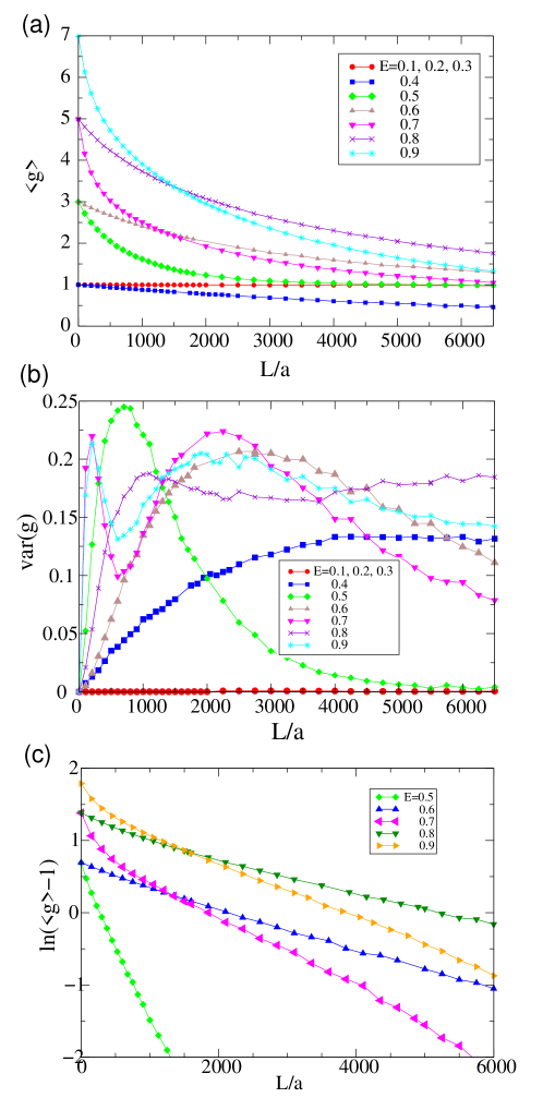
Figure 3: $L$-dependence of (a) the average, $\langle g\rangle$, (b) the corresponding variance, $var(g)$, and (c) corresponding log-plot $\ln\langle g-1\rangle$ of dimensionless conductance for zigzag ribbon with $N=10$, $d/a=1.5$ (no inter-valley scattering), $u_{0}=1.0$, and $n_{imp.}=0.1$. More than 9000 samples with different impurity configuration are included in the ensemble average.

We organize this paper as follows. In Sec. 2, we briefly introduce the electronic states of graphene nanoribbons with zigzag edges. In Sec. 3, some peculiar features in the scattering matrix formulation on the graphene nanoribbons are explained, where the non-square form of the reflection matrix and the implications of the perfectly conducting channel in nanoribbons are presented. Also, the results of numerical calculation are shown. In Sec. 4, we discuss the electronic states of graphene nanoribbons with general edge structures, and demonstrate that chiral channels due to the edge states is realized even in the general edge structures except for the armchair edge. In Sec. 5, the universality class of the nanographene ribbons is discussed. The conclusion is presented in Sec. 6.

II Electronic states

We describe the electronic states of nanographites by the tight-binding model

$$H=\sum_{i,j}\gamma_{i,j}|i\rangle\langle j|+\sum_{i}V_{i}|i\rangle\langle i|,$$ (1)

where $\gamma_{i,j}=-1$ if $i$ and $j$ are nearest neighbors, and 0 otherwise. $|i\rangle$ represents the state of the $p_{z}$-orbital on site $i$ neglecting the spin degrees of freedom. In the following we will also apply magnetic fields perpendicular to the graphite plane which are incorporated via the Peierls phase:

$$\gamma_{i,j}\rightarrow\gamma_{i,j}\exp\left[i2\pi\frac{e}{ch}\int_{i}^{j}d\bm{l\cdot A}\right],$$ (2)

where $\bm{A}$ is the vector potential. The second term in Eq. (1) represents the impurity potential, $V_{i}=V(\bm{r}_{i})$ is the impurity potential at a position $\bm{r}_{i}$.

In Fig.1(a), the graphite ribbon with zigzag edges (zigzag ribbons ) is shown. We assume edge sites are terminated by H-atoms. The ribbon width $N$ is defined by the number of zigzag lines. The length of disordered region is defined as $L$. Fig. 1(b) depicts the energy band structure of zigzag ribbon for $N=10$. The zigzag ribbons are metallic for arbitrary ribbon width. The most remarkable feature is the presence of a partly flat band at the Fermi level, where the electrons are strongly localized near the zigzag edge. Each edge state has a non-vanishing amplitude only on one of the two sublattices, having, thus, non-bonding character. However, in a zigzag ribbon of finite width, two edge states coming from both sides, have finite overlap. Because they are located on different sublattices, they mix into a bonding and anti-bonding configuration. In this way the partly flat bands acquire a dispersion and become conductive except at exactly $E=0$. Note that the overlap is increasing as $k$ deviates from $\pm\pi/a$, because the penetration depth of the edge states increases and diverges at $k=\pm 2\pi/3a$, where $a$ is the lattice constant.

We briefly discuss here the relation between valleys in the zigzag ribbons and two-dimensional graphene. The electronic states near the Dirac point can be described by the $\bm{k\cdot p}$ Hamiltonian

$$H_{\bm{k\cdot p}}=\tilde{\gamma}\left[\hat{k}_{x}(\sigma^{x}\otimes\tau^{0})+\hat{k}_{y}(\sigma^{y}\otimes\tau^{z})\right]$$ (3)

acting on the 4-component pseudo-spinor Bloch functions $\Phi(\bm{r})=\left[\phi_{\bm{K_{+}}A},\phi_{\bm{K_{+}}B},\phi_{\bm{K_{-}}A},\phi_{\bm{K_{-}}B}\right]$, which characterize the wave functions on the two crystalline sublattices (A and B) for the two Dirac points (valleys) $\bm{K}_{\pm}$. Here, $\tilde{\gamma}$ is the band parameter, $\hat{k}_{x}$($\hat{k}_{y}$) are wavenumber operators, and $\tau^{0}$ is the $2\times 2$ identity matrix. Pauli matrices $\sigma^{x,y,z}$ act on the sublattice space ($A$, $B$), while $\tau^{x,y,z}$ on the valley space ($\bm{K}_{\pm}$). Since the outermost sites along $1^{st}$ ($N^{th}$) zigzag chain are B(A)-sublattice, an imbalance between two sublattices occurs at the zigzag edges leading to the boundary conditions

$$\phi_{\bm{K_{\pm}}A}(\bm{r}_{[0]})=0,\quad\phi_{\bm{K_{\pm}}B}(\bm{r}_{[N+1]})=0,$$ (4)

where $\bm{r}_{[i]}$ stands for the coordinate at $i^{th}$ zigzag chain. It can be shown that the valley near $k=3\pi/2a$ in Fig.1(b) originates from the $\bm{K_{+}}$-point, the other valley at $k=-3\pi/2a$ from $\bm{K_{-}}$-point.Phd ; note.bc ; luis

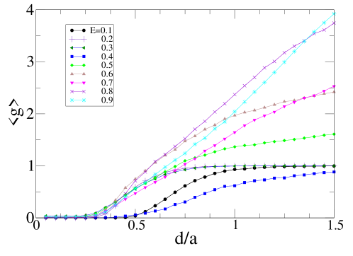
Figure 4: Impurity range, $d/a$, dependence of the averaged dimensionless conductance, $\langle g\rangle$, for zigzag ribbon with $N=10$, $u_{0}=1.0$, $L/a=5000$ and $n_{imp.}=0.1$. More than 1000 samples with different impurity configuration are included in the ensemble average.

Since the momentum difference between two valleys is rather large, $\Delta k=k_{+}-k_{-}=4\pi/3a$, only short-range impurities (SRI) with a range smaller than the lattice constant causes inter-valley scattering. Long-range impurities (LRI), in contrast, restrict the scattering processes to intra-valley scattering. ando.nakanishi

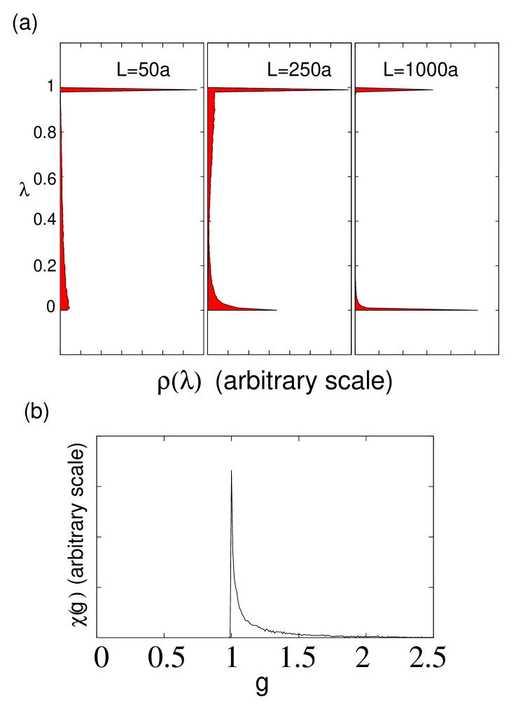
Figure 5: (a) Distribution of the transmission eigenvalues $\lambda$: $\rho(\lambda)$, at $E=0.5$ for $L/a=50,250,1000$, with $d/a=2.0$. $E=0.5$ leads to 3 incident channels. 12,000 samples with different impurity configurations are included in the distribution. (b) Distribution of the dimensionless conductance $g$: $\chi(g)$, at $L/a=1000$ for the same parameter set.

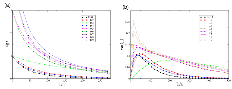
Figure 6: $L$-dependence of (a) the averaged dimensionless conductance and (b) the variance of the conductance for zigzag ribbons with $N=10$, short-ranged impurity potential ($d/a=0.05$, inter-valley scattering), $u_{0}=1.0$, and $n_{imp.}=0.1$. 20000 samples with different impurity configurations are in the ensemble average.

In the graphene systems, pairs of time-reversed states are formed across the two valleys (Dirac points). In the absence of inter-valley scattering for LRI, this ordinary TRS becomes irrelevant, while the pseudo time-reversal symmetry with respect to the operator $\mathcal{T}=-i(\sigma_{y}\otimes\tau_{0})C$ ($C$: complex conjugation) appears, where the A-B sublattices act as pseudospin. This corresponds to the time-reversal operation restricted to each valley. The boundary conditions which treat the two sublattices asymmetrically leading to edge states give rise to a single special mode in each valley. Considering now one of the two valleys separately, say the one around $k=k_{+}$, we see that the pseudo TRS is violated in the sense that we find one more left-moving than right-moving mode. Thus, as long as disorder promotes only intra-valley scattering, the system has no time-reversal symmetry. On the other hand, if disorder yields inter-valley scattering, the pseudo TRS disappears but the ordinary TRS is relevant making a complete set of pairs of time-reversed modes across the two valleys. Thus we expect to see qualitative differences in the properties if the range of the impurity potentials is changed.

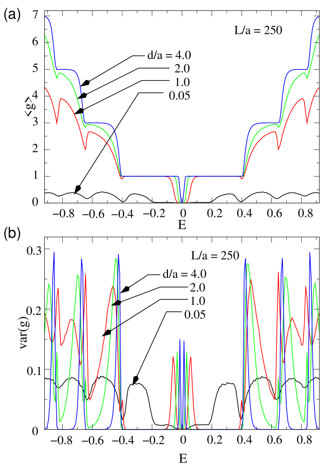
Figure 7: Fermi energy dependence of (a) the averaged dimensionless conductance and (b) the variance of the conductance for zigzag ribbons with $N=10$ for various impurity potential ranges at $L/a=250$. 10000 samples with different impurity configurations are in the ensemble average. Here, $u_{0}=1.0$ and $u_{imp.}=0.1$.

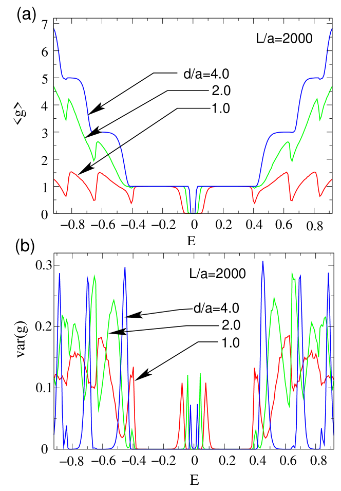
Figure 8: Fermi energy dependence of (a) the averaged dimensionless conductance and (b) the variance of the conductance for zigzag ribbons with $N=10$ for various impurity potential ranges at $L/a=2000$. 3200 samples with different impurity configurations are in the ensemble average. In this regime the averaged conductance for short-ranged impurities($d/a\ll 1$) is zero. Here, $u_{0}=1.0$ and $u_{imp.}=0.1$.

III Electronic transport properties

III.1 One-way excess channel system

We numerically discuss the electronic transport properties of the disordered nanographene ribbons. In general, electron scattering in a quantum wire is described by the scattering matrix.beenakker.rmt Through the scattering matrix $\bm{S}$, the amplitudes of the scattered waves $\bm{O}$ are related to the incident waves $\bm{I}$,

$$\left(\begin{array}[]{c}\bm{O_{L}}\\ \bm{O_{R}}\end{array}\right)=\bm{S}\left(\begin{array}[]{c}\bm{I_{L}}\\ \bm{I_{R}}\end{array}\right)=\left(\begin{array}[]{cc}\bm{r}&\bm{t^{\prime}}\\ \bm{t}&\bm{r^{\prime}}\end{array}\right)\left(\begin{array}[]{c}\bm{I_{L}}\\ \bm{I_{R}}\end{array}\right).$$ (5)

Here, $\bm{r}$ and $\bm{r^{\prime}}$ are reflection matrices, $\bm{t}$ and $\bm{t^{\prime}}$ are transmission matrices, $L$ and $R$ denote the left and right lead lines. The Landauer-Büttiker formulamclbf relates the scattering matrix to the conductance of the sample. The electrical conductance is calculated using the Landauer-Büttiker formula,

$$G(E)=\frac{e^{2}}{\pi\hbar}{\rm Tr}(\bm{t}\bm{t}^{\dagger})=\frac{e^{2}}{\pi\hbar}g(E).$$ (6)

Here the transmission matrix $\bm{t}(E)$ can be calculated by means of the recursive Green function method.prl ; prb ; green2 For simplicity, throughout this paper, we evaluate electronic conductance in the unit of quantum conductance ($e^{2}/\pi\hbar$), i.e. dimensionless conductance $g(E)$. We would like to mention that recently the edge disorder effect on the electronic transport properties of graphene nanoribbons was studied using similar approach.li ; louis ; mucciolo

In the clean limit, the conductance of the zigzag ribbon can be given simply by the number of the conducting channel. As can be seen in Fig. 1(b), there is always one excess left-going channel in the right valley ($\bm{K_{+}}$) within the energy window of $|E|\leq 1$. Analogously, there is one excess right-going channel in the left valley ($\bm{K_{-}}$) within the same energy window. Although the number of right-going and left-going channels are balanced as a whole system, however if we focus on one of two valleys, there is always one excess channel in one direction, i.e. chiral mode.

Now let us inject electrons from left to right-side through the sample. When the chemical potential is changed from $E=0$, the quantization rule of the dimensionless conductance ($g_{\bm{K_{+}}}$) in the valley of $\bm{K_{+}}$ is given as

$$g_{\bm{K_{+}}}=n,$$ (7)

where $n=0,1,2,\cdots$. The quantization rule in the $\bm{K_{-}}$-valley is

$$g_{\bm{K_{+}}}=n+1.$$ (8)

Thus, conductance quantization of the zigzag ribbon in the clean limit near $E=0$ has the following odd-number quantization, i.e.

$$g=g_{\bm{K_{+}}}+g_{\bm{K_{-}}}=2n+1.$$ (9)

Since we have an excess mode in each valley, the scattering matrix has some peculiar features which can be seen when we explicitly write the valley dependence in the scattering matrix. By denoting the contribution of the right valley ($\bm{K_{+}}$) as $+$, and of the left valley ($\bm{K_{-}}$) as $-$, the scattering matrix can be rewritten as

$$\left(\begin{array}[]{c}\bm{O^{+}_{L}}\\ \bm{O^{-}_{L}}\\ \bm{O^{+}_{R}}\\ \bm{O^{-}_{R}}\end{array}\right)=\left(\begin{array}[]{cc}\bm{r}&\bm{t^{\prime}}\\ \bm{t}&\bm{r^{\prime}}\end{array}\right)\left(\begin{array}[]{c}\bm{I^{+}_{L}}\\ \bm{I^{-}_{L}}\\ \bm{I^{+}_{R}}\\ \bm{I^{-}_{R}}\end{array}\right).$$ (10)

Here we should note that the dimension of each column vector is not identical. Let us denote the number of the right-going channel in the valley $\bm{K_{+}}$ or the left-going channel in the valley $\bm{K_{-}}$ as $n_{c}$. For example, $n_{c}=1$ at $E=E_{0}$ in the Fig.1(b). Thus the dimension of the column vectors is given as follows:

$$\left\{\begin{array}[]{ll}dim(\bm{I^{+}_{L}})=n_{c},&dim(\bm{I^{+}_{R}})=n_{c}+1,\\ dim(\bm{I^{-}_{L}})=n_{c}+1,&dim(\bm{I^{-}_{R}})=n_{c},\\ \end{array}\right.$$ (11)

and

$$\left\{\begin{array}[]{ll}dim(\bm{O^{+}_{L}})=n_{c}+1,&dim(\bm{O^{+}_{R}})=n_{c},\\ dim(\bm{O^{-}_{L}})=n_{c},&dim(\bm{O^{-}_{R}})=n_{c}+1.\\ \end{array}\right.$$ (12)

Subsequently, the reflection and transmission matrices have the following matrix structures,

$$\bm{r}=\bordermatrix{&n_{c}&n_{c}+1\cr n_{c}+1&\bm{r_{++}}&\bm{r_{+-}}\cr n_{c}&\bm{r_{-+}}&\bm{r_{--}}},$$ (13)

$$\bm{t}=\bordermatrix{&n_{c}&n_{c}+1\cr n_{c}&\bm{t_{++}}&\bm{t_{+-}}\cr n_{c}+1&\bm{t_{-+}}&\bm{t_{--}}},$$ (14)

$$\bm{r^{\prime}}=\bordermatrix{&n_{c}+1&n_{c}\cr n_{c}&\bm{r^{\prime}_{++}}&\bm{r^{\prime}_{+-}}\cr n_{c}+1&\bm{r^{\prime}_{-+}}&\bm{r^{\prime}_{--}}},$$ (15)

$$\bm{t^{\prime}}=\bordermatrix{&n_{c}+1&n_{c}\cr n_{c}+1&\bm{t^{\prime}_{++}}&\bm{t^{\prime}_{+-}}\cr n_{c}&\bm{t^{\prime}_{-+}}&\bm{t^{\prime}_{--}}}.$$ (16)

The reflection matrices become non-square when the intervalley scattering is suppressed, i.e. the off-diagonal submatrices are zero.

When the electrons are injected from the left lead of the sample and the intervalley scattering is suppressed, a system with an excess channel is realised in the $\bm{K_{-}}$-valley. The scattering geometry is schematically drawn in Fig.2. Thus, for single valley transport, the $\bm{r_{--}}$ and $\bm{r^{\prime}_{--}}$ are $n_{c}\times(n_{c}+1)$ and $(n_{c}+1)\times n_{c}$ matrices, respectively, and $\bm{t_{--}}$ and $\bm{t^{\prime}_{--}}$ are $(n_{c}+1)\times(n_{c}+1)$ and $n_{c}\times n_{c}$ matrices, respectively. Noting the dimensions of $\bm{r_{--}}$ and $\bm{r^{\prime}_{--}}$, we find that $\bm{r_{--}}^{\dagger}\bm{r_{--}}$ and $\bm{r^{\prime}_{--}}{\bm{{r^{\prime}}^{\dagger}_{--}}}$ have a single zero eigenvalue. Combining this with the flux conservation relation ($\bm{S}^{\dagger}\bm{S}=\bm{S}\bm{S}^{\dagger}=\bm{1}$), we arrive at the conclusion that $\bm{t_{--}t^{\dagger}_{--}}$ has an eigenvalue equal to unity. Note that ${\bm{t^{\prime}}_{--}}{\bm{t^{\prime}}}^{\dagger}_{--}$ does not have such an anomalous eigenvalue. This indicates the presence of a perfectly conducting channel (PCC) only in the right-moving channels. If the set of eigenvalues for ${\bm{t^{\prime}}_{--}}{\bm{t^{\prime}}}^{\dagger}_{--}$ is expressed as $\{T_{1},T_{2},\cdots,T_{n_{c}}\}$, that for ${\bm{t_{--}}{\bm{t}}^{\dagger}_{\bm{-}-}}$ is expressed as $\{T_{1},T_{2},\cdots,T_{n_{c}},1\}$, i.e. a PCC. Thus, the dimensionless conductance g for the right-moving channels is given as

$$g_{\bm{K_{-}}}=\sum_{i=1}^{n_{c}+1}T_{i}=1+\sum_{i=1}^{n_{c}}T_{i},$$ (17)

while that for the left-moving channels is

$$g^{\prime}_{\bm{K_{-}}}=\sum_{i=1}^{n_{c}}T_{i}.$$ (18)

We see that $g_{\bm{K_{-}}}=g^{\prime}_{\bm{K_{-}}}+1$. Since the overall TRS of the system guarantees the following relation:

$$\begin{array}[]{c}g^{\prime}_{\bm{K_{+}}}=g_{\bm{K_{-}}},\\ g^{\prime}_{\bm{K_{-}}}=g_{\bm{K_{+}}},\end{array}$$ (19)

the conductance $g=g_{\bm{K_{+}}}+g_{\bm{K_{-}}}$ (right-moving) and $g^{\prime}=g^{\prime}_{\bm{K_{+}}}+g^{\prime}_{\bm{K_{-}}}$ (left-moving) are equivalent. If the probability distribution of $\{T_{i}\}$ is obtained as a function $L$, we can describe the statistical properties of $g$ as well as $g^{\prime}$. The evolution of the distribution function with increasing $L$ is described by the DMPK(Dorokhov-Mello-Pereyra-Kumar) equation for transmission eigenvalues.takane4

In the following, the presence of a perfectly conducting channel in disordered nanographene ribbons will be demonstrated with the help of numerical calculation. Recently Hirose et. al. pointed out that the Chalker-Coddington model which possesses non-square reflection matrices with unitary symmetry gives rise to a perfectly conducting channel.ohtsuki However, systems with an excess channel in one direction has been believed difficult to realize. Therefore disordered nanographene ribbons with LRI might constitute the first realistic example. It is possible to extend the discussion to generic multiple-excess channel model, where the $m$-PCCs appear.takane4 Such systems can be realized by stacking zigzag nanographene ribbons.miyamoto The electronic transport due to PCC resembles to the electronic transport due to a chiral mode in quantum Hall system.macdonald ; ishizaka However, it should be noted that the PCC due to edge states in zigzag ribbons occurs even without the magnetic field.

III.2 model of impurity potential

In our model we assume that the impurities are randomly distributed with a density $n_{imp}$, and the potential has a Gaussian form of a range $d$

$$V(\bm{r}_{i})=\sum_{\bm{r_{0}}(random)}u\exp\left(-\frac{|\bm{r}_{i}-\bm{r}_{0}|^{2}}{d^{2}}\right)$$ (20)

where the strength $u$ is uniformly distributed within the range $|u|\leq u_{M}$. Here $u_{M}$ satisfies the normalization condition:

$$u_{M}\sum_{{\bm{r}}_{i}}^{(full\ space)}\exp\left(-{\bm{r}_{i}^{2}}{d^{2}}\right)/(\sqrt{3}/2)=u_{0}.$$ (21)

Since the momentum difference between two valleys is rather large, $\Delta k=k_{+}-k_{-}=4\pi/3a$, only short-range impurities (SRI) with a range smaller than the lattice constant causes inter-valley scattering. Long-range impurities (LRI), in contrast, restrict the scattering processes to intra-valley scattering.ando.nakanishi

III.3 disordered nanographene ribbons

We focus first on the case of LRI using a potential with $d/a=1.5$ which is already sufficient to avoid inter-valley scattering. Fig.3 shows (a) the averaged dimensionless conductance and (b) the corresponding variance as a function of $L$ for different incident energies, averaging over an ensemble of 40000 samples with different impurity configurations for ribbons of the width $N=10$. The variance, which describes the fluctuation of the conductance, is defined as

$$var(g)=\langle g^{2}\rangle-\langle g\rangle^{2}.$$ (22)

The potential strength and impurity density are chosen to be $u_{0}=1.0$ and $n_{imp.}=0.1$, respectively. As a typical localization effect we observe that $\langle g\rangle$ gradually decreases with growing length $L$ (Fig.3). Surprisingly, the ribbons remain highly conductive even at the length of $L=1500a$, i.e. more than $350nm$ in the real system. Actually, $\langle g\rangle$ converges to $\langle g\rangle=1$, indicating the presence of a single perfectly conducting channel. It can be seen that $\langle g\rangle(L)$ has an exponential behavior as

$$\langle g\rangle-1\sim\exp(-L/\xi)$$ (23)

with $\xi$ as the localization length. In this paper, the localization length is evaluated, by identifying $\exp\langle\ln\tilde{g}\rangle=\exp(-L/\xi)$. Here, $\tilde{g}=g-1$ ($\tilde{g}=g$) for the system with (without) the perfectly conducting channel.

Interestingly, the variance for the LRI case shown in Fig.3(b) has large values and slowly converges to zero toward the long wire limit. Also, the variance for higher energy modes has double humps structure in the short wire regime, which is also indicating the unconventional behavior. Such suppression of the fluctuation in the diffusive regime may be attributed to the level repulsion from the transmission eigenvalue of the PCC.preprint Note the variance is zero for $E=0.1,0.2,0.3$, indicating the existence of the perfectly conducting channel. Such peculiar features cannot be seen for SRI case, see Fig.6(b) for comparison.

Fig.4 shows impurity range ($d/a$) dependence of the averaged conductance for various Fermi energy. Clearly, it can be seen that the PCC develops in zigzag ribbons if the range of impurity gets larger than the lattice constant. However, the development of PCC gets moderate if the incident energy lies at a value close to the change between $g=2n-1$ and $g=2n+1$ for the ribbon without disorder. Since at least one of subbands at these energy points gives zero group velocity, it can be considered that the intra-valley scattering becomes stronger. This feature is also for example visible in above calculations as the deviation from the limit $\langle g\rangle\to 1$ for $E=0.4$ where the limiting value $\langle g\rangle<1$ (Fig.3). This feature can be seen clearly in Fig.7 and 8, which will be discussed later.

We performed a number of tests to confirm the presence of this perfectly conducting channel. First of all, it exists up to $L=3000a$ for various ribbon widths up to $N=40$ for the potential range ($d/a=1.5$). Moreover the perfectly conducting channel remains for LRI with $d/a=2.0,4.0,6.0,8.0$, and $u_{0}=1.0$, $n_{imp.}=0.1$ and $N=10$. As the effect is connected with the subtle feature of an excess mode in the band structure, it is natural that the result can only be valid for sufficiently weak potentials. For potential strengths comparable to the energy scale of the band structure, e.g. the energy difference between the transverse modes, the result should be qualitatively altered.vacancy

As a further test we evaluate the distribution of the transmission eigenvalues and dimensionless conductance for fixed wire length. In Fig.5(a), the distribution of the eigenvalues $\lambda$ of the Hermite matrix, $\bm{tt}^{\dagger}$, is depicted for various wire lengths. With growing length $L$ a progressive separation of the transmission eigenvalues emerges with a strong peak close to 0 (localization) and at 1 (perfect conduction channel). The distribution of the conductance $g$ (trace of the transmission matrix ${\rm Tr}(\bm{tt}^{\dagger})$), is depicted in Fig.5(b) for samples in the long-wire limit. Obviously, $g$ only distributes above $g=1$ with a singularity at 1.

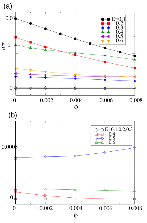
Figure 9: (a) Magnetic field dependence of the inverse localization length $\xi^{-1}$ for various incident energies. The filled symbols indicate data sets of systems with SRI being rather sensitive to magnetic fields, and empty symbols denote data sets for LRI which are almost insensitive to the field. The magnetic flux $\phi$ passing through a single hexagon ring is measured in units of the quantum flux ($\phi_{0}=ch/e$). (b) Enlarged view of (a) of LRI data 5000 samples with different configurations are included in the averages.

Turning to the case of SRI the inter-valley scattering becomes sizable enough to ensure TRS, such that the perfect transport supported by the effective chiral mode in a single valley ceases to exist. For a comparison, we show the ribbon length dependence of the averaged conductance in Fig.6. Since SRI causes the inter-valley scattering for any incident energy, the electrons tend to be localized and the averaged conductance decays exponentially, $\langle g\rangle\sim\exp(-L/\xi)$, without developing a perfect conduction channel.

In Fig.7, Fermi energy dependence of (a) the averaged dimensionless conductance and (b) the variance of the conductance for zigzag ribbons with $N=10$ for various impurity potential ranges $d/a=0.05,1.0,2.0,4.0$ at $L/a=250$. 10000 samples with different impurity configurations are in the ensemble average. With decreasing the range of the impurity potential, the averaged conductance also gradually decreases and the perfect conduction disappears for short-ranged impurities of $d/a=0.05$. As we have already briefly mentioned, the sharp dips can be observed at energies where the number of conducting channels changes. Also, the variances becomes relatively large at these energies. The drop of the conductance close to E=0 indicates that the two valleys are not well-separated in $k$-space, because the partial flat bands have finite curvature for narrow graphene ribbons such as $N=10$. Therefore, if the ribbon width widens, the perfectly conduction recovers even close to the zero-energy. In Fig.8, similar figure for $L/a=2000$.

In order to demonstrate that the qualitative difference between the two regimes, LRI and SRI, is indeed connected with TRS, we study the effect of magnetic field coupling to the electrons through the Peierls phase. For the time reversal symmetric situation resulting from SRI scattering the magnetic field removing TRS should have a stronger effect than for the case of LRI where TRS is broken already at the outset. We use the localization length $\xi$ as an indicator. In Fig.9, the field dependence of the inverse localization length is shown for various incident energies (filled symbols for SRI and empty symbols for LRI). Indeed the localization length displays a stronger field dependence than the LRI. Actually for LRI even a so-called anti-localization behavior with increasing field is visible consistent with recent reports on graphene.antilocalization ; suzuura.prl ; prb Note that for $E<0.4$ only a single channel is involved in the conductance such that for LRI no localization occurs, i.e. $\xi^{-1}=0$.

IV General edge structures

As we have seen, zigzag ribbons with long-ranged impurity potentials retain a single PCC. This PCC originates for the following two reasons: (i) The spectrum contains two valleys (two Dirac $\bm{K_{\pm}}$-points) which are well enough separated in momentum space as to suppress intervalley scattering due to the long-ranged impurities, (ii) the spectrum in each valley is chiral by possessing a right- and left-moving modes which differ by one in number, and so scattered electrons can avoid in one channel backscattering. Is the zigzag ribbon the only nanographene ribbon showing this effect? Here we would like to show that such conditions can be satisfied in the graphene nanoribbon with more general edge structures except for one case, the armchair edge. In the following we will first show that only the armchair edge cannot produce the localized edge states. Moreover, the spectrum of the armchair ribbon overlays the two Dirac $\bm{K}$-points at the single momentum $k=0$ and displays therefore no separation into two valleys unlike the zigzag ribbon. We will then show that general edges can produce the necessary conditions to observe a PCC in a disordered system.

IV.1 Continuum approach

We consider graphene at half-filling in order to explore their zero-energy edge states. Here from the tight-binding model we derive the stationary Schrödinger equation for graphene in momentum space,

$$\left[\begin{array}[]{cc}0&\epsilon_{\bm{k}}^{\ast}\\ \epsilon_{\bm{k}}&0\end{array}\right]\hat{\Psi}_{\bm{k}}=E\hat{\Psi}_{\bm{k}}$$ (24)

where $\epsilon_{\bm{k}}=-t\sum_{i}\exp(i\bm{k\cdot\tau_{i}})$ ($\bm{\tau}_{1}=a(0,1/\sqrt{3})$, $\bm{\tau}_{2}=a(-1/2,-1/2\sqrt{3})$, and $\bm{\tau}_{3}=a(1/2,-1/2\sqrt{3})$) and

$$\hat{\Psi}_{\bm{k}}=\left(\begin{array}[]{c}\psi_{A}({\bm{k}})\\ \psi_{B}({\bm{k}})\end{array}\right)$$ (25)

with $\psi_{A}(\bm{k})$ and $\psi_{B}(\bm{k})$ are the wavefunctions located on the A- and B-sublattice, respectively. The spectrum contains the well-known linear Dirac spectrum at two nonequivalent momentum $\bm{K_{\pm}}$ points, $\bm{K}_{\pm}=\frac{2\pi}{a}(\pm\frac{1}{3},\frac{1}{\sqrt{3}})$. In Fig.10, (a) the lattice structure of graphene and the definition of $\bm{\tau}_{i}$($i=1,2,3$) and coordinates, (b) corresponding 1st Brillouin Zone, and (c) $\pi$ band structures are shown.

In a first discussion concerning edge states we perform the following transformation:

$$\hat{\Phi}_{\bm{k}}=\left(\begin{array}[]{c}\phi_{p}(\bm{k})\\ \phi_{h}(\bm{k})\end{array}\right)=\frac{1}{\sqrt{2}}\left(\begin{array}[]{c}\psi_{A}(\bm{k})+\psi_{B}(\bm{k})\\ i\psi_{B}(\bm{k})-i\psi_{A}(\bm{k})\end{array}\right)$$ (26)

which yields the Schrödinger equation,

$$(\epsilon^{+}_{\bm{k}}\hat{\sigma}_{z}-i\epsilon^{-}_{\bm{k}}\hat{\sigma}_{x})\hat{\Phi}_{\bm{k}}=E\hat{\Phi}_{\bm{k}},$$ (27)

where $\epsilon^{\pm}_{\bm{k}}=(\epsilon_{\bm{k}}\pm\epsilon_{\bm{k}}^{\ast})/2$. The structure of this equation is identical to that of a BCS problem in particle-hole space $(\psi_{p},\psi_{h})$, constituting a Bogolyubov-de Gennes equation. The diagonal terms, $\epsilon^{+}_{\bm{k}}={\rm Re}(\epsilon_{\bm{k}})$, formally correspond to the kinetic energy for particles and holes, and the off-diagonal terms, $-i\epsilon^{-}_{\bm{k}}={\rm Im}(\epsilon_{\bm{k}})$, can be considered as the pair-potential of a ”superconductor”.

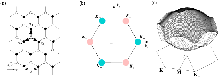
Figure 10: (a) The lattice structure of graphene and the definition of $\tau_{i}$ ($i=1,2,3$) and coordinates. Here $\bm{\tau}_{1}=a(0,1/\sqrt{3})$, $\bm{\tau}_{2}=a(-1/2,-1/2\sqrt{3})$, and $\bm{\tau}_{3}=a(1/2,-1/2\sqrt{3})$. (b) The corresponding 1st Brillouin Zone. $\bm{K}_{\pm}=\frac{2\pi}{a}(\pm\frac{1}{3},\frac{1}{\sqrt{3}})$, $\bm{\Gamma}=(0,0)$, and so on. (c) The band energy structures for $\pi$ electrons.

Figure 11: The contour plot for (a) $\epsilon^{+}_{\bm{k}}$ (b) $\Delta_{\bm{k}}$. The dashed line means the negative values.

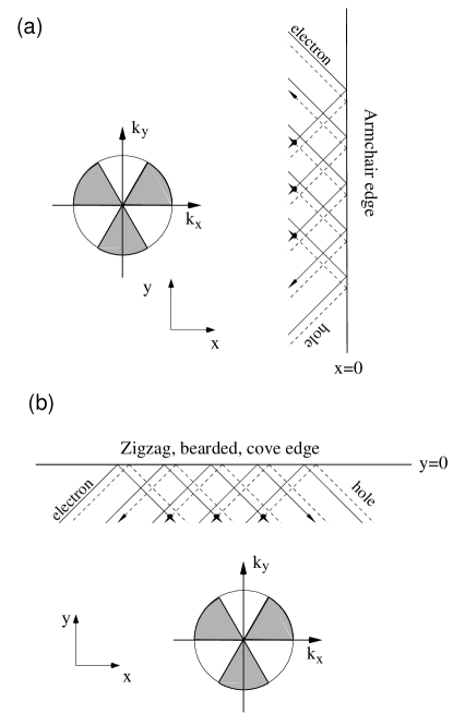
Figure 12: Schematic view of the electron scattering in the surface region of graphene with the analogy to the Andreev reflection, where the electronic states of graphene were mapped to the picture of the $f$-wave superconductors(see text). Circles with shading shows the wavenumber dependence of $\Delta_{\bm{k}}$, where shading means negative values. (a) The scattering trajectories at the armchair edge, which convert the momentum as $k_{x}\rightarrow-k_{x}$, do not connect gap regions of opposite sign. However, (b) The scattering trajectories at the zigzag, bearded and cove edge, which convert the momentum as $k_{y}\rightarrow-k_{y}$, connect gap regions of opposite sign which lead to a phase shift $\pi$ and zero-energy bound states.

Thus we rewrite the equation as

$$(\hat{\xi}_{\bm{k}}\hat{\sigma}_{z}+\Delta_{\bm{k}}\hat{\sigma}_{x})\hat{\Phi}_{\bm{k}}=E\hat{\Phi}_{\bm{k}}\;.$$ (28)

In the continuum limit we can approximate $\hat{\xi}_{\bm{k}}=-({\hbar^{2}}/{2m})\nabla^{2}-\mu$, where $\mu$ is the chemical potential, and $\Delta_{\bm{k}}$ represents the pair-potential of the superconductor, $\Delta_{\bm{k}}=\left(\epsilon_{\bm{k}}-\epsilon_{\bm{k}}^{\ast}\right)/2i={\rm Im}(\epsilon_{\bm{k}})$. In Fig.11, the contour plot for (a) $\epsilon^{+}_{\bm{k}}$ (b) $\Delta_{\bm{k}}$ are shown. The pair potential shows line nodes along the momenta $k_{y}=\pm\sqrt{3}k_{x}$ and $k_{y}=0$. Thus close to the Fermi energy we approximate the pair potential simply by its angular dependence

$$\Delta=|\Delta|\cos(3\theta),$$ (29)

where $\theta$ is the angle of the Fermi vector relative to the positive $k_{x}$-axis. Interestingly, the ”pairing” symmetry is odd-parity, an $f$-wave state.

From this properties we use now the general rules for the presence of zero-energy edge states.hu ; kashiwaya A related discussion can be found in ref.ryu . Considering a classical trajectory, the existence of a zero-energy bound state requires that the momentum incident to the edge and the momentum of specular scattered outgoing trajectory lie on the Fermi surface on points which have a phase difference of $\pi$ for the pair potential. Fig.12 shows that this condition is satisfied for the zigzag edge, i.e. $\Delta(k_{x},-k_{y})=-\Delta(k_{x},k_{y})$. On the other hand, the phase difference is zero for the armchair edge, i.e. $\Delta(-k_{x},k_{y})=\Delta(k_{x},k_{y})$. Thus we do not expect zero-energy bound states in the latter case. The condition that there are no trajectories with a $\pi$-phase difference is only satisfied for the armchair edge.

This conclusion is consistent with the results of tight binding model.nakada ; ezawa Also, similar conclusion has been recently given by the approach of $\bm{k\cdot p}$ equation by Akhmerov.akhmerov The electronic properties of nanoribbons with clean edge based on the $\bm{k\cdot p}$ equation can be found in ref.Phd ; luis .

Let us now turn to the original two-sublattice representation and consider the continuum limit in order to analyze possible surface bound states. For zigzag edges the $x$-axis is taken to lie parallel to the edge and the $y$-axis parallel to the normal vector. Along the edge we choose the momentum $k_{x}$. Expanding around the $K_{+}$-point we separate the fast oscillating part by introducing $p_{y}=k_{x}-2\pi/\sqrt{3}a$. Then, we write the wave function as

$$\psi_{A(B)}(\bm{r})=f_{A(B)}(y){\rm e}^{ik_{x}x}{\rm e}^{i\frac{2\pi}{\sqrt{3}a}y},$$ (30)

where $f_{A(B)}(y)$ describes the slow $y$-dependence. Concentrating on the energy close to zero we can also take the linear momentum dependence along the $y$-direction so that the effective Hamiltonian has the form

$$\left[\begin{array}[]{cc}0&h_{AB}\\ h_{BA}&0\end{array}\right]\left(\begin{array}[]{c}f_{A}(y)\\ f_{B}(y)\\ \end{array}\right)=E\left(\begin{array}[]{c}f_{A}(y)\\ f_{B}(y)\\ \end{array}\right),$$ (31)

where

$$h_{BA}=h_{AB}^{*}=-t{\rm e}^{-i\frac{\pi}{3}}\left[D_{k_{x}}-1-i\frac{a}{\sqrt{3}}\left\{\frac{D_{k_{x}}}{2}+1\right\}\hat{p}_{y}\right]$$ (32)

with $D_{k_{x}}=2\cos(k_{x}a/2)$. Now we replace $\hat{p}_{y}=-i\partial_{y}$ and formulate the differential equations for $f_{A(B)}(y)$. The outer-most lattice sites on the zigzag edge belong to one sublattice only, say the $B$-sublattice. Then we take the $A$-sublattice wave function to vanish $f_{A}(y)=0$. For the zero-energy $E=0$ we analyze the equation for $f_{B}$ which reads now

$$\partial_{y}f_{B}(y)=-\frac{\sqrt{3}}{a}\frac{D_{k}-1}{1+\frac{D_{k}}{2}}f_{B}(y)\equiv\alpha_{B}(k_{x})f_{B}(y)\;.$$ (33)

This equation has an exponentially decaying bound-state solution $f_{B}(y)=C{\rm e}^{\alpha_{B}y}$ whose existence condition is $\alpha_{B}(k_{x})>0$, resulting in $|k_{x}|\geq 2\pi/3$. As $k_{x}$ approaches $2\pi/3$ the bound state extends deeper into the bulk, because its extension is given by

$$\ell(k_{x})=\frac{a}{\sqrt{3}}\frac{1+\cos(k_{x}a/2)}{1-2\cos(k_{x}a/2)}.$$ (34)

Analogous conditions can be found for other related edges, such as the bearded edge where $f_{B}(y)=0$. Then we obtain zero-energy bound states for $\alpha_{A}=-\alpha_{B}>0$ which leads to the condition $|k_{x}|\leq 2\pi/3$ consistent with numerical calculations for the tight-binding model.

Now we turn to the armchair edge which extends along the $y$-axis. Both $\bm{K_{+}}$ and $\bm{K_{-}}$ are projected on the same point in $k_{y}$-momentum space. Analogous to the zigzag edge we expand the wavefunction around one of the two points, say $\bm{K_{-}}=\frac{2\pi}{a}\left(\frac{2}{3},0\right)$ and write

$$\psi_{A(B)}(\bm{r})=f_{A(B)}(x){\rm e}^{ik_{y}y}{\rm e}^{i\frac{4\pi}{3a}x}.$$ (35)

where we extract again the fast oscillating part along the $x$-axis normal to the edge. We linearize again the spectrum close to zero energy and take $p_{x}=k_{x}-4\pi/3a$. Then, for $f_{A(B)}$, the Hamiltonian has the form

$$\left[\begin{array}[]{cc}0&h_{AB}\\ h_{BA}&0\end{array}\right]\left(\begin{array}[]{c}f_{A}(x)\\ f_{B}(x)\\ \end{array}\right)=E\left(\begin{array}[]{c}f_{A}(x)\\ f_{B}(x)\\ \end{array}\right),$$ (36)

where

$$h_{BA}=h_{AB}^{*}=-t{\rm e}^{-ik_{y}a/6}\left[{\rm e}^{-ik_{y}a/2}-1-\frac{a}{2}\hat{p}_{x}\right].$$ (37)

where we redefined the unit length as $a\equiv\sqrt{3}a$ which corresponding to the length of the translational vector for armchair ribbons. Using $\hat{p}_{y}=-i\partial_{y}$ and making the ansatz

$$\left(\begin{array}[]{c}f_{A}(x)\\ f_{B}(x)\end{array}\right)\sim\left(\begin{array}[]{c}\phi_{A}\\ \phi_{B}\end{array}\right){\rm e}^{\lambda x}\;.$$ (38)

The boundary condition for the armchair edge require $\left(\phi_{A},\phi_{B}\right)\neq 0$ as we will see. For $E=0$, the $\lambda$ has two solutions

$$\begin{array}[]{cl}\lambda_{\pm}&=-i\frac{4}{a}\sin^{2}\frac{ka}{4}\pm\frac{2}{a}\sin\frac{ka}{2}\\ &\equiv-i\eta\pm\zeta.\end{array}$$ (41)

and leads to the wavefunction,

$$\left(\begin{array}[]{c}f_{A}(x)\\ f_{B}(x)\end{array}\right)=\left(\begin{array}[]{c}\phi^{+}_{A}\\ \phi^{+}_{B}\end{array}\right){\rm e}^{\lambda_{+}x}+\left(\begin{array}[]{c}\phi^{-}_{A}\\ \phi^{-}_{B}\end{array}\right){\rm e}^{\lambda_{-}x},$$ (42)

the coefficients are determined to satisfy the condition that the dimensionless electronic current normal to the edge vanishes, i.e. $j_{x}=0$ with

$$\begin{array}[]{cl}j_{x}=&\Psi^{\dagger}\sigma_{x}\Psi\\ =&f^{\ast}_{B}(x)f_{A}(x)+f^{\ast}_{A}(x)f_{B}(x).\end{array}$$ (45)

This leads to the solution

$$\left(\begin{array}[]{c}\psi_{A}\\ \psi_{B}\end{array}\right)=\frac{1}{\sqrt{2}}\left(\begin{array}[]{c}i\\ 1\end{array}\right){\rm e}^{ik_{y}y}{\rm e}^{\frac{4\pi}{3a}x}{\rm e}^{-i\eta x}\cosh\zeta x.$$ (46)

It is easy to see by inserting this wavefunction into the Schrödinger equation that the only zero-energy states is obtained for $k_{y}=0$ for which $\eta=0$. Thus no zero-energy bound state exists in the case of the armchair edge.

IV.2 Spectrum and valley structure of other edges

We now analyze the energy band structure of graphene nanoribbons with general edge structures based on the tight-binding model. We will show that the appearance of flat bands is a general features (apart from armchair ribbons) and yield a two-valley structure with chiral edge states similar to the case of zigzag edges.

IV.2.1 Bearded Edge and Cove Edge

We start our discussion with the most simple edge shapes having translational symmetry along the zigzag axis, called bearded and cove. Although these two edges look rather artificial compared with the zigzag edge, they are interesting because they show very much the same non-bonding edge localization as the standard zigzag edge.

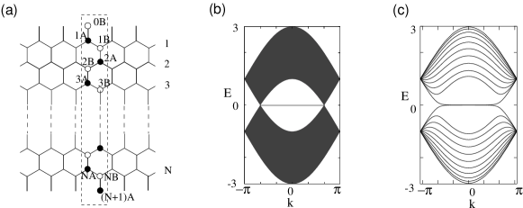
Figure 13: (a) The structure of a graphite ribbon with two bearded edges. (b) The band structure of a semi-infinite graphite sheet with a bearded edge. (c) The band structure of bearded ribbon for $N=10$.

A bearded edge is derived from a zigzag edge by adding single $\pi$-electron hopping bonds on each boundary site as shown in Fig.13(a). This type of edge was first studied by Klein.klein In Fig.13(b), the band structure of a semi-infinite graphite sheet with a bearded edge is shown. Interestingly, a partial flat band appears in the region of $|k|\leq 2\pi/3$, which is the opposite condition in the semi-infinite graphite sheet with a zigzag edge, as we had anticipated by our continuum approximation above.

It is interesting to consider a ribbon having one edge of zigzag and the other of bearded shape as shown in Fig.14(a). Because for this ribbon $|N_{\rm A}-N_{\rm B}|=1$, where $N_{\rm A}(N_{\rm B})$ means the number of sites belonging to the A(B)-sublattice, there is a flat band at $E=0$ all over the 1st BZ, as shown in Fig.14(b). The analytic solution of this flat band can be easily understood by the combination of two edge states for zigzag and bearded edges. In the region of $|k|<2\pi/3$, the electrons are localized at the bearded edge, and in the region of $|k|>2\pi/3$, the electrons are localized at the zigzag edge. At $k=\pm 2\pi/3$, the wavefunctions extend over the whole ribbon width. It should be noted that this ribbon is insulating at half-filling because the flat band has no dispersion and, thus, cannot carry currents. Moreover, there is an energy gap between the flat band and next subbands.

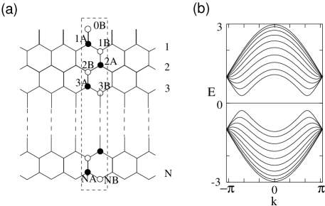
Figure 14: (a) The structure of a graphite ribbon with a zigzag and a bearded edge and (b) the band structure for $N=10$.

Cove edge is a zigzag edge with additional hexagon rings attached. A graphene ribbon with two cove edges is shown in Fig.15(a). In Fig.15(b), the band structure of a semi-infinite graphite sheet with a cove edge is shown. This case also provides a partly flat band in the region of $|k|\leq 2\pi/3$ like the zigzag edge.

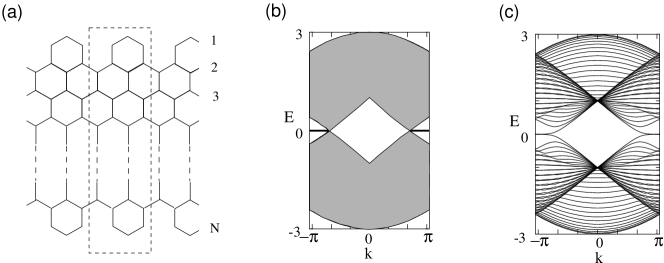
Figure 15: (a) The structure of a graphite ribbon with two cove edges. (b) The band structure of a semi-infinite graphite sheet with a cove edge. (c) The band structure of bearded ribbon for $N=10$.

Interestingly both bearded and cove graphene ribbons posses two well-separated valleys in momentum space and chiral modes in both due to the partially flat bands. Thus in both case PCC are realized as long as the impurity potential is long-ranged.

IV.2.2 General ribbons with $|N_{A}-N_{B}|=0$

We extend our analysis to the electronic spectrum of nanoribbons for which the ribbon axis is tilted with respect to the zigzag axis and keep the balance between $A$- and $B$-sublattice sites.

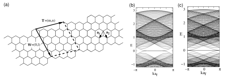
Figure 16: (a) The primitive vectors for nanoribbon with the general edge structures. The translational vector is defined as $\bm{T}=(m,n)=m\bm{a_{1}}+n\bm{a_{2}}$, and the ribbon width is defined by the vector $\bm{W}=(0,l)=l\bm{a_{2}}$. The number of carbon atoms in the unit cell is $2(l+1)m$. The corresponding energy band structures of $\bm{W}=(0,20)$ for (b) $\bm{T}=(-4,3)$ and (c) $\bm{T}=(-6,5)$. Here $a_{T}$ is the effective lattice constant which is given as $|\bm{T}|$.

In Fig.16(a), we show the definitions of coordinates and primitive vectors which specifies the geometry of the ribbon. For this purpose we introduce the two vectors, $\bm{T}=(m,n)=m\bm{a_{1}}+n\bm{a_{2}}$ and $\bm{W}=(0,l)=l\bm{a_{2}}$, where $l,m,n$ are integers. The pure zigzag ribbon corresponds to $m=-n$ and the pure armchair edge is given by $m=n$.

Fig.16(b) and (c) show the energy band structures of ribbons with the general edge structures of $\bm{W}=(0,20)$ and (b) $\bm{T}=(-4,3)$ and (c) $\bm{T}=(-6,5)$ are shown. As we expected, the partially flat bands due to localized edge modes appear which break the balance between left- and right-going modes in the two valleys. Both examples are rather close to the zigzag edge so that the two valleys are well separated. In this case PCC can appear. If the geometry of the ribbons deviates more strongly from the zigzag condition, the valley structure will become less favorable for creating a PCC, as the momentum difference between valleys shrinks. It is important to note that the extended unit cell along these generalized ribbons reduces the valley separation drastically through Brillouin zone folding. The length scale is the new effective lattice constant $a_{T}$ along the ribbon.　 Under these circumstances the condition for long-ranged impurity potentials is more stringent, $d$ being larger than $a_{T}$ and not $a$.

V Universality class

According to random matrix theory, ordinary disordered quantum wires are classified into the standard universality classes, orthogonal, unitary and symplectic. The universality classes describe transport properties which are independent of the microscopic details of disordered wires. These classes can be specified by time-reversal and spin rotation symmetry(Table 1). The orthogonal class consists of systems having both time-reversal and spin-rotation symmetries, while the unitary class is characterized by the absence of time-reversal symmetry. The systems having time-reversal symmetry without spin-rotation symmetry belong to the symplectic class. These universality classes have been believed to inevitably cause the Anderson localization although typical behaviors are different from class to class.

Table 1: Universality class

Universality	TRI	SRI
Orthogonal	Yes	Yes
Unitary	No	irrelevant
Symplectic	Yes	No

Recently, the presence of one perfectly conducting channel has been found in disordered metallic carbon nanotubes with LRI.suzuura The PCC in this system originates from the skew-symmetry of the reflection matrix, ${}^{t}\bm{r}=-{\bm{r}}$,suzuura which is special to the symplectic symmetry with odd number of channels. The electronic transport properties such system has been studied on the basis of the random matrix theory.takane1 ; takane2 On the other hand, zigzag ribbons without inter-valley scattering are not in the symplectic class, since they break TRS in a special way. The decisive feature for a perfectly conducting channel is the presence of one excess mode in each valley as discussed in the previous section.

In view of this classification we find that the universality class of the disordered zigzag ribbon with long-ranged impurity potential (no inter-valley scattering) is the unitary class (no TRS). On the other hand, for short-range impurity potentials with inter-valley scattering the disordered ribbon belongs to the orthogonal class (with overall TRS). This classification is compatible with the magnetic field dependence of the localization length $\xi$ as shown in Fig.9. Consequently we can observe a crossover between two universality classes when we change the impurity range continuously.

Figure 17: Summary concerning for the universality crossover. With increasing the range of the impurity potential, graphene is known to be the orthogonal for SRIs and the symplectic class for LRIs. However, zigzag nanoribbons are unitary class for SRIs. Armchair ribbons are irrelevant for the range of the impurity. $L_{\phi}$ is the phase coherence length. $W$ is the width of graphene ribbons.

Analogous symmetry considerations can be applied to armchair ribbons. In this case the two valleys merge into a single one at $k=0$. TRS is conserved irrespective of the impurity potential range, if there is no magnetic field. Consequently, disordered armchair ribbons belong always to the orthogonal class and do not provide a perfectly conducting channel. In view of the fact that graphene is known to be symplectic (orthogonal) for LRI (SRI),suzuura.prl it is quite intriguing to realize that the edges influence the universality class, as long as the phase coherence length is larger than the system characteristic size of the nanographene system. In the Fig.17, the summary of the argument is visualized. In the nano-graphene ribbons with general edges, since the two Dirac points are separated in the momentum space with the order of $|1/\bm{T}|$, the characteristic length causing the crossover is $\sim|\bm{T}|$. Thus the PPC is expected to appear even in generic nanoribbons if the sample has only very slowly varying charge potential and the intervalley scattering is suppressed.

VI Conclusion

The unusual energy dispersion due to their edge states gives rise to the unique property of zigzag ribbons. Concerning transport properties for disordered systems the most important consequence is the presence of a perfectly conducting channel, i.e. the absence of Anderson localization which is believed to inevitably occur in the one-dimensional electron system. The origin of this effect lies in the single-valley transport which is dominated by a chiral mode. On the other hand, large momentum transfer through impurities with short-range potentials involves both valleys, destroying this effect and leading to usual Anderson localization. The obvious relation of the chiral mode with time reversal symmetry leads to the classification into the unitary and orthogonal class depending on the range of impurity potential. Since the inter-valley scattering is weak in the experiments of graphene, we may assume that these conditions may be realized also for ribbons. Naturally defects in the ribbon edges and vacancies would be rather harmful for the experiment making this type of experiment very challenging.prl ; prb

References

- (1) Novoselov KS, Geim AK, Morozov SV, Jian D, Zhang Y, Dubonos SV, et. al., Electric Field Effect in Atomically Thin Carbon Films, Science 2004; 306: 666-669.
- (2) Geim AK, MacDonald AH, Graphene: Exploring Carbon Flatland, Phys. Today, 2007; 60: 35-41.
- (3) Novoselov KS, Geim AK, Morozov SV, Jiang D, Katsnelson MI, Grigorieva IV, et. al., Two-Dimensional Gas of Massless Dirac Fermions in Graphene, Nature 2005; 438: 197-200
- (4) Zhang Y, Tan YW, Stormer HL, Kim P, Experimental observation of the quantum Hall effect and Berry’s phase in graphene, Nature 2005; 438: 201-204
- (5) Ando T, Nakanishi T, Impurity Scattering in Carbon Nanotubes – Absence of Back Scattering –, J. Phys. Soc. Jpn. 1998; 67: 1704-1708
- (6) Luk’yanchuk IA, Kopelevich Y, Phase Analysis of Quantum Oscillations in Graphite, Phys. Rev. Lett. 2004; 93: 166402(1)-166402(4)
- (7) Fujita M, Wakabayashi K, Nakada K, Kusakabe K, Peculiar Localized State at Zigzag Graphite Edge, J. Phys. Soc. Jpn. 1996; 65: 1920-1923
- (8) Wakabayashi K, Fujita M, Ajiki H, Sigrist M, Electronic and Magnetic Properties of Nanographite Ribbons, Phys. Rev. B 1999; 59: 8271-8282
- (9) Wakabayashi K, Low-Energy Physical Properties of Edge States in Nano-Graphites, Univ. of Tsukuba, PhD thesis, 2000. http://www.tulips.tsukuba.ac.jp/dspace/handle/2241/2592
- (10) Kobayashi Y, Fukui K, Enoki T, Kusakabe K, Kaburagi Y, Observation of zigzag and armchair edges of graphite using scanning tunneling microscopy and spectroscopy, Phys. Rev. B 2005; 71: 193406(1)-193406(4)
- (11) Niimi Y, Matsui T, Kambara H, Tagami K, Tsukada M, Fukuyama H, Scanning tunneling microscopy and spectroscopy of the electronic local density of states of graphite surfaces near monoatomic step edges, Phys. Rev. B 2006; 73: 085421(1) - 085421(8)
- (12) Han MY, Özyilmaz B, Zhang Y, Kim P, Energy Band-Gap Engineering of Graphene Nanoribbons, Phys. Rev. Lett, 2007; 98: 206805 (1) - 206805 (4).
- (13) Wakabayashi K, Sigrist M, Zero-Conductance Resonances due to Flux States in Nanographite Ribbon Junctions, Phys. Rev. Lett. 2000; 84: 3390-3393
- (14) Wakabayashi K, Electronic Transport Properties of Nano-Graphite Ribbon Junctions, Phys. Rev. B 2001; 64: 125428 (1) - 125428 (15)
- (15) Wakabayashi K, Numerical study of the lattice vacancy effects on the single-channel electron transport of nanographite ribbons, J.Phys.Soc. Jpn. 2002; 71: 2500-2504
- (16) Rycerz A, Tworzydlo J, Beenakker CWJ, Valley filter and valley valve in graphene Nat. Phys. 2007; 3: 172 - 175
- (17) Son YW, Cohen ML, and Louie SG, Half-metallic graphene nanoribbons, Nature 2006; 444: 347 - 349
- (18) Kane CL, Mele EJ, Quantum Spin Hall Effect in Graphene, Phys. Rev. Lett. 2005; 95: 226801(1) - 226801(4)
- (19) Kusakabe K, Maruyama M, Magnetic nanographite, Phys. Rev. B 2003; 67: 092406(1)-092406(4)
- (20) Okada S, Energetics of nanoscale graphene ribbons: Edge geometries and electronic structures, Phys. Rev. B 2008; 77: 041408(1)-041408(4).
- (21) Harigaya K, Enoki T, Mechanism of magnetism in stacked nanographite with open shell electrons Chem. Phys. Lett. 2002; 351: 128-134
- (22) Takai K, Eto S, Inaguma M, Enoki T, Ogata H, Tokita M, et.al., Magnetic Potassium Clusters in a Nanographite Host System, Phys. Rev. Lett. 2007; 98: 017203(1)-017203(4)
- (23) Palacios JJ, Fernández-Rossier and L. Brey, Vacancy-induced magnetism in graphene and graphene ribbons, Phys. Rev. B 2008; 77: 195428(1)-195428(14)
- (24) Ando T, Suzuura H, Presence of Perfectly Conducting Channel in Metallic Carbon Nanotubes, J. Phys. Soc. Jpn. 2002; 71: 2753-2760
- (25) Wakabayashi K, Takane Y, Sigrist M, Perfectly Conducting Channel and Universality Crossover in Disordered Graphene Nanoribbons, Phys. Rev. Lett. 2007; 99: 036601(1)-036601(4)
- (26) Takane Y, DMPK Equation for Transmission Eigenvalues in Metallic Carbon Nanotubes, J. Phys. Soc. Jpn. 2004; 73: 9-12
- (27) Sakai H, Takane Y, Random-Matrix Theory of Electron Transport in Disordered Wires with Symplectic Symmetry, J. Phys. Soc. Jpn. 2005; 75: 054711(1)-054711(5)
- (28) Hirose K, Ohtsuki T, Slevin K, Quantum transport in novel Chalker-Coddington model, Physica E 2008; 40: 1677-1680
- (29) Takane Y, Wakabayashi K: Conductance of Disordered Wires with Unitary Symmetry: Role of Perfectly Conducting Channels, J. Phys. Soc. Jpn. 2007; 76: 053701(1)-053701(4)
- (30) Beenakker CWJ, Random-matrix theory of quantum transport, Rev. Mod. Phys. 1997; 69: 731-808
- (31) Note two virtual zigzag chains on both sides are necessary for the boundary condition on zigzag ribbon of width .
- (32) Brey L, Fertig HA, Electronic states of graphene nanoribbons studied with the Dirac equation, Phys. Rev. B 2006; 73: 235411(1)-235411(5)
- (33) Büttiker M, Imry Y, Landauer R, Pinhas S, Generalized many-channel conductance formula with application to small rings, Phys. Rev. B 1985; 31: 6207-6215
- (34) Ando T, Quantum point contacts in magnetic fields, Phys. Rev. B 1991; 44: 8017-8027
- (35) Li TC, and Lu SP, Quantum conductance of graphene nanoribbons with edge defects, Phys. Rev. B 2008; 77; 085408(1)-085408(5)
- (36) Louis E, Vergés JA, Guinea F, and Chiappe G, Transport regimes in surface disordered graphene sheets, Phys. Rev. B 2007; 75; 085440(1)-085440(5)
- (37) Mucciolo ER, Castro Neto AH, Lewenkopf CH, cond-mat/0806.3777
- (38) Miyamoto Y, Nakada K, Fujita M, First-principles study of edge states of H-terminated graphitic ribbons, Phys. Rev. B 1999; 59: 9858-9861
- (39) MacDonald AH, Edge states and quantized Hall conductivity in a periodic potential, Phys. Rev. B 1984; 29: 6563-6569
- (40) Ishizaka S, Nakamura K, Ando T, Edge states and quantized Hall resistance in quantum wires containing a periodic potential, Phys. Rev. B 1993; 48: 12053-12062
- (41) Takane Y, Wakabayashi K, Conductance Fluctuations in Disordered Wires with Perfectly Conducting Channels, J. Phys. Soc. Jpn. 2008; 77: 054702(1)-054702(6)
- (42) McCann E, Kechedzhi K, Fal’ko VI, Suzuura H, Ando T, Altshuler BL, Weak-Localization Magnetoresistance and Valley Symmetry in Graphene, Phys. Rev. Lett. 2005; 97: 146805(1) - 146805(4)
- (43) Suzuura H, Ando T, Crossover from Symplectic to Orthogonal Class in a Two-Dimensional Honeycomb Lattice, Phys. Rev. Lett. 2002; 89: 266603 (1) - 266603 (4)
- (44) Hu CR, Midgap surface states as a novel signature for -wave superconductivity, Phys. Rev. Lett. 1994; 72: 1526-1529
- (45) Kashiwaya S, Tanaka Y, Tunnelling effects on surface bound states in unconventional superconductors, Rep. Prog. Phys. 2000; 63: 1641-1724
- (46) Ryu S, Hatsugai Y, Topological Origin of Zero-Energy Edge States in Particle-Hole Symmetric Systems, Phys. Rev. Lett. 2002; 89: 077002(1)-077002(4)
- (47) Nakada K, Fujita M, Dresselhaus G, Dresselhaus MS, Edge state in graphene ribbons: Nanometer size effect and edge shape dependence, Phys. Rev. B 1996; 54: 17954-17961
- (48) Ezawa M, Peculiar width dependence of the electronic properties of carbon nanoribbons, Phys. Rev. B 2006; 73: 045432(1)-045432(8)
- (49) Akhmerov AR, Beenakker CWJ, Boundary conditions for Dirac fermions on a terminated honeycomb lattice, Phys. Rev. B 2008; 77: 085423(1)-085423(10).
- (50) Klein DJ, Graphitic polymer strips with edge states, Chem. Phys. Lett. 1994; 217: 261-265