Loop-erased random walk and Poisson kernel on planar graphs

Abstract

Lawler, Schramm and Werner showed that the scaling limit of the loop-erased random walk on $\mathbb{Z}^{2}$ is $\mathrm{SLE}_{2}$. We consider scaling limits of the loop-erasure of random walks on other planar graphs (graphs embedded into $\mathbb{C}$ so that edges do not cross one another). We show that if the scaling limit of the random walk is planar Brownian motion, then the scaling limit of its loop-erasure is $\mathrm{SLE}_{2}$. Our main contribution is showing that for such graphs, the discrete Poisson kernel can be approximated by the continuous one.

One example is the infinite component of super-critical percolation on $\mathbb{Z}^{2}$. Berger and Biskup showed that the scaling limit of the random walk on this graph is planar Brownian motion. Our results imply that the scaling limit of the loop-erased random walk on the super-critical percolation cluster is $\mathrm{SLE}_{2}$.

and

1 Introduction

Let $G$ be a graph. The loop-erased random walk or LERW on $G$ is obtained by performing a random walk on $G$, and then erasing the loops in the random walk path in chronological order. The resulting path is a self-avoiding path in the graph $G$, starting and ending at the same points as the random walk. LERW was invented by Lawler in LERWdfn as a natural measure on self-avoiding paths. It was studied extensively on the graphs $\mathbb{Z}^{d}$. In dimensions $d\geq 4$, the scaling limit is known to be Brownian motion (see LawlerSurvey ). In dimension $d=3$, Kozma proved that the scaling limit exists and that the limit is invariant under rotations and dilations (see Kozma ). In order to study the case $d=2$, in SchSLE Schramm introduced a one-parameter family of random continuous curves, known as Schramm–Loewner evolution or $\mathrm{SLE}_{\kappa}$. In LSW Lawler, Schramm and Werner proved that the scaling limit of LERW on $\mathbb{Z}^{2}$ is $\mathrm{SLE}_{2}$. Their result also holds for other two-dimensional lattices. Many other processes in statistical mechanics have been shown to converge to $\mathrm{SLE}_{\kappa}$ for other values of $\kappa$.

In this paper, we focus on the scaling limit of LERW on planar graphs, not necessarily lattices. A planar graph is a graph embedded into the complex plane so that edges do not intersect each other; a precise definition is provided in Section 1.1. We allow weighted and directed graphs, but require them to be irreducible; that is, any two points are connected by a path in the graph.

Our main result, Theorem 1.1, is a generalization of LSW . Let $G$ be an irreducible graph, and let $f\dvtx G\to\mathbb{C}$ be an embedding of $G$ into the complex plane. If $f(G)$ is planar (in the sense above), and if the scaling limit of the random walk on $f(G)$ is planar Brownian motion, then the scaling limit of LERW on $f(G)$ is $\mathrm{SLE}_{2}$.

One interesting example is the infinite component of super-critical percolation on $\mathbb{Z}^{2}$. That is, consider bond percolation on $\mathbb{Z}^{2}$, each bond open with probability $p>1/2$, all bonds independent. Then, a.s. there exists a unique infinite connected component. In BerBisk Berger and Biskup proved that a.s. the scaling limit of the random walk on this infinite component is Brownian motion. Together with our result, this implies that a.s. the scaling limit of LERW on the super-critical percolation cluster is $\mathrm{SLE}_{2}$ (see Figure 1).

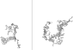
Figure 1: LERW (black) and simple random walk (gray) stopped on exiting the unit disc. The underlying graphs are $\mathbb{Z}^{2}$ (left) and the super-critical percolation cluster with parameter $0.75$ (right). The mesh size is $1/600$.

Another example of a planar graph with random walk converging to planar Brownian motion is given by Lawler in LawRWRE (see the example following Lemma 5). For each vertex $z\in\mathbb{Z}^{2}$, define transition probabilities as follows: the probability to go either up or down is $p(z)/2$, and the probability to go either left or right is $(1-p(z))/2$. Lawler proved in LawRWRE that if $p(z)$ are all chosen i.i.d. such that $\mathbb{P}[p(z)=p]=\mathbb{P}[p(z)=1-p]=1/2$, for some $0<p<1/2$, then a.s. the scaling limit of the random walk on this graph is planar Brownian motion. Our result implies that the LERW on this graph converges to $\mathrm{SLE}_{2}$.

The main contribution of this work is Lemma 1.2, that states that for planar graphs, the discrete Poisson kernel can be approximated by the continuous Poisson kernel. This result holds for any bounded domain, although the boundary behavior can be arbitrary. This result also holds “pointwise,” regardless of the local geometry of the graph. Perhaps it can be used to generalize other limit theorems about processes on $\mathbb{Z}^{2}$ (such as IDLA) to more general planar graphs (e.g., the super-critical percolation cluster).

1.1 Definitions and notation

For any $v,u\in\mathbb{C}$, denote $[v,u]=\{(1-t)v+tu\dvtx 0\leq t\leq 1\}$.

Planar-irreducible graphs

Let $G=(V,E)$ be a directed weighted graph; that is, $E\dvtx V\times V\to[0,\infty)$. We write $(v,u)\in E$, if $E(v,u)>0$. Let $o\in V$ be a fixed vertex. Let $f\dvtx V\to\mathbb{C}$ be an embedding of $G$ in the complex plane such that: [(1)]

$f(o)=0$.

The embedding of $G$ in $\mathbb{C}$ is a “planar” graph; that is, for every two edges $(v,u),(v^{\prime},u^{\prime})\in E$ such that $\{v,u\}\cap\{v^{\prime},u^{\prime}\}=\varnothing$, $[f(v),f(u)]\cap[f(v^{\prime}),f(u^{\prime})]=\varnothing$.

For every compact set $K\subset\mathbb{C}$, the number of vertices $v\in V$ such that $f(v)\in K$ is finite. We think of the graph $G$ as its embedding in $\mathbb{C}$. For $\delta>0$, let $G_{\delta}=(V_{\delta},E_{\delta})$ be the graph defined by

$$V_{\delta}=\{\delta f(v)\dvtx v\in V\}\quad\mbox{and}\quad E_{\delta}(\delta f(v),\delta f(u))=E(v,u);$$

that is, $G_{\delta}$ is the embedding of $G$ in $\mathbb{C}$ scaled by a factor of $\delta$.

We assume that $\sum_{u\in V}E(v,u)<\infty$ for every $v\in V$. Let $P\dvtx V\times V\to[0,1]$ be

$$P(v,u)=\frac{E(v,u)}{\sum_{w\in V}E(v,w)}.$$

We call the Markov chain induced on $V_{\delta}$ by $P$ the natural random walk on $G_{\delta}$. We assume that the natural random walk is irreducible; that is, for every $v,u\in V$, there exists $n\in\mathbb{N}$ such that $P^{n}(v,u)>0$.

We call a graph $G$ that satisfies all the above properties a planar-irreducible graph. For the remainder of this paper we consider only planar-irreducible graphs.

Loop erasure

Let $x(0),x(1),\ldots,x(n)$ be $n+1$ vertices in $G_{\delta}$. Define $x[0,n]$ as the linear interpolation of $(x(0),\ldots,x(n))$; that is, for $t\in[0,n]$, set

$$x(t)=\bigl{(}1-(t-\lfloor t\rfloor)\bigr{)}x(\lfloor t\rfloor)+(t-\lfloor t\rfloor)x(\lfloor t\rfloor+1).$$

Define the loop-erasure of $x(\cdot)$ as the self-avoiding sequence induced by erasing loops in chronological order; that is, the loop-erasure of $x(\cdot)$ is the sequence $y(\cdot)$ that is defined inductively as follows: $y(0)=x(0)$, and $y(k+1)$ is defined using $y(k)$ as $y(k+1)=x(T+1)$, where $T=\max\{\ell\leq n\dvtx x(\ell)=y(k)\}$ [the loop-erasure ends once $y(k)=x(n)$].

A path from $v$ to $u$ in $G_{\delta}$ is a sequence $v=x(0),x(1),\ldots,x(n)=u$ such that $(x(j),x(j+1))\in E_{\delta}$ for all $j$. The reversal of the path $x(\cdot)$ is the sequence $x(n),x(n-1),\ldots,x(0)$. The reversal of a path is not necessarily a path.

Domains

Denote by $\mathbb{U}$ the open unit disc in $\mathbb{C}$. Let $D\subsetneqq\mathbb{C}$ be a simply connected domain such that $0\in D$. Define $V_{\delta}(D)$ as the set of vertices $z\in V_{\delta}\cap D$ such that there is a path from $0$ to $z$ in $G_{\delta}$. Define

$$\partial V_{\delta}(D)=\{(v,u)\dvtx(v,u)\in E_{\delta},v\in V_{\delta}(D),[v,u]\cap\partial D\neq\varnothing\},$$

the “boundary” of $G_{\delta}$ in $D$. Denote by $\varphi_{D}\dvtx D\to\mathbb{U}$ the unique conformal map onto the unit disc such that $\varphi_{D}(0)=0$ and $\varphi_{D}^{\prime}(0)>0$. Define the inner radius of $D$ as $\operatorname{rad}(D)=\sup\{R\geq 0\dvtx R\cdot\mathbb{U}\subseteq D\}$.

Throughout this paper, we work with a fixed domain and its sub-domains. Fix a specific bounded domain $\mathbf{D}\subsetneqq\mathbb{C}$ such that $\operatorname{rad}(\mathbf{D})>1/2$ (one can think of $\mathbf{D}$ as $\mathbb{U}$). Denote

$$\mathfrak{D}=\{D\subseteq{\mathbf{D}}\dvtx D\mbox{ simply connected domain},\operatorname{rad}(D)>1/2\}.$$

SLE

Radial $\mathrm{SLE}_{\kappa}$ in $\mathbb{U}$ can be described as follows (for more details see, e.g., LawlerBook , LSW , RS01 , SchSLE , Werner ). Let $\gamma$ be a simple curve from $\partial\mathbb{U}$ to $0$. Parameterize $\gamma$ so that $g^{\prime}_{t}(0)=e^{t}$, where $g_{t}$ is the unique conformal map mapping $\mathbb{U}\setminus\gamma[0,t]$ onto $\mathbb{U}$ with $g_{t}(0)=0$ and $g^{\prime}_{t}(0)>0$. It is known that the limit $W(t)=\lim_{z\to\gamma(t)}g_{t}(z)$ exists, where $z$ tends to $\gamma(t)$ from within $\mathbb{U}\setminus\gamma[0,t]$. In addition, $W\dvtx[0,\infty)\to\partial\mathbb{U}$ is a continuous function, and the Loewner differential equation is satisfied

$$\partial_{t}g_{t}(z)=g_{t}(z)\frac{W(t)+g_{t}(z)}{W(t)-g_{t}(z)}$$

and $g_{0}(z)=z$. The function $W(\cdot)$ is called the driving function of $\gamma$.

Taking $W(t)=e^{iB(\kappa t)}$, where $B(\cdot)$ is a one-dimensional Brownian motion (started uniformly on $[0,2\pi]$), one can solve the Loewner differential equation, obtaining a family of conformal maps $g_{t}$. It turns out that for $\kappa\leq 4$, the curve $\gamma$ obtained from the driving function $W$ (defined as $\gamma(0)=W(0)$ and $\gamma(0,t]=\mathbb{U}\setminus g^{-1}_{t}(\mathbb{U})$) is indeed a simple curve from $\partial\mathbb{U}$ to $0$ (see RS01 ). The curve $\gamma$ is called the $\mathrm{SLE}_{\kappa}$ path.

Weak convergence

We define weak convergence using one of several equivalent definitions (see Chapter III in Shiry , e.g.). Let $\alpha,\beta\dvtx[0,1]\to\mathbb{U}$ be two continuous curves. Let $\Phi$ be the set of continuous nondecreasing maps $\phi\dvtx[0,1]\to[0,1]$. We say that $\alpha$ and $\beta$ are equivalent if $\alpha=\beta\circ\phi$ for some $\phi\in\Phi$. Let $\mathcal{C}$ be the set of all equivalence classes under this relation. Define $\varrho(\alpha,\beta)=\inf_{\phi\in\Phi}\sup_{t\in[0,1]}|\alpha(t)-\beta(\phi(t))|$.

It is known that $\varrho(\cdot,\cdot)$ is a metric on $\mathcal{C}$. Let $\Sigma$ be the Borel $\sigma$-algebra generated by the open sets of $\varrho$. Let $\mu$ be a probability measure on $(\mathcal{C},\Sigma)$. We say that $A\in\Sigma$ is $\mu$-continuous, if $\mu(\partial A)=0$, where $\partial A$ is the boundary of $A$.

Let $\{\mu_{n}\}$ be a sequence of probability measures on $(\mathcal{C},\Sigma)$. We say that $\{\mu_{n}\}$ converges weakly to $\mu$, if for all $\mu$-continuous events $A\in\Sigma$, it holds that $\mu_{n}(A)$ converges to $\mu(A)$.

Poisson kernel

Let $D\in\mathfrak{D}$. For $a\in V_{\delta}(D)$ and $b\in V_{\delta}(D)\cup\partial V_{\delta}(D)$, define $H(a,b)=H^{(\delta)}(a,b;D)$ to be the probability that a natural random walk on $G_{\delta}$, started at $a$ and stopped on exiting $D$, visits $b$. That is,

$$H(a,b)=\cases{\mathbb{P}[\exists 0\leq k\leq\tau\dvtx S(k)=b],&\quad$b\in V_{\delta}(D)$,\cr\mathbb{P}\bigl{[}\bigl{(}S(\tau-1),S(\tau)\bigr{)}=b\bigr{]},&\quad$b\in\partial V_{\delta}(D)$,}$$

where $S(\cdot)$ is a natural random walk on $G_{\delta}$ started at $a$, and $\tau$ is the exit time of $S(\cdot)$ from $D$. We sometimes denote the segment $(S(\tau-1),S(\tau))$ by $S(\tau)$; for example, instead of $(S(\tau-1),S(\tau))=b$ we write $S(\tau)=b$, and for a set $J\subseteq\partial D$, we write $S(\tau)\in J$ instead of writing $[S(\tau-1),S(\tau)]\cap J\neq\varnothing$.

Let $e=(v,u)\in\partial V_{\delta}(D)$. Let $\tilde{e}\in\partial D$ be the “first” point on the $[v,u]$ that is not in $D$; that is, let $s=\inf\{0\leq t\leq 1\dvtx(1-t)v+tu\notin D\}$, and let $\tilde{e}=(1-s)v+su$. Define $\varphi(e)=\lim_{t\to s^{-}}\varphi((1-t)v+tu)$.

For $a\in V_{\delta}(D)$ and $b\in V_{\delta}(D)\cup\partial V_{\delta}(D)$, define the Poisson kernel

$$\lambda(a,b)=\lambda(a,b;D)=\frac{1-|\varphi(a)|^{2}}{|\varphi(a)-\varphi(b)|^{2}}.$$

If $B(\cdot)$ is a planar Brownian motion started at $x\in\mathbb{U}$, $\tau$ is the exit time of $B(\cdot)$ from $\mathbb{U}$, and $J$ is a Borel subset of $\partial\mathbb{U}$, then

$$\mathbb{P}_{x}[B(\tau)\in J]=\int_{J}\lambda(x,\zeta;\mathbb{U})\,d\zeta,$$ (1)

where $d\zeta$ is the uniform measure on $\partial\mathbb{U}$ (see Chapter 3 of PeresBM ).

Complex analysis

Throughout the proofs we will make repeated use of three classical theorems in the theory of analytic and conformal maps: the Schwarz lemma, the Koebe distortion theorem and the Koebe $1/4$ theorem. These can be found in Conway or Pom .

1.2 Main results

Let $G$ be a planar-irreducible graph. Let $\nu_{\delta}$ be the law of the natural random walk on $G_{\delta}$ started at $0$ and stopped on exiting $\mathbb{U}$. Let $\mu_{\delta}$ be the law of the loop-erasure of the reversal of the natural random walk on $G_{\delta}$ started at $0$ and stopped on exiting $\mathbb{U}$.

Theorem 1.1

Let $\{\delta_{n}\}$ be a sequence converging to $0$. If $\nu_{\delta_{n}}$ converges weakly to the law of planar Brownian motion started at $0$ and stopped on exiting $\mathbb{U}$, then $\mu_{\delta_{n}}$ converges weakly to the law of radial $\mathrm{SLE}_{2}$ in $\mathbb{U}$ started uniformly on $\partial\mathbb{U}$.

The proof of Theorem 1.1 is given in Section 6. A key ingredient in the proof is the following lemma, that shows that the discrete Poisson kernel can be approximated by the continuous one (its proof is given in Section 5).

Lemma 1.2

For all $\varepsilon,\alpha>0$, there exists $\delta_{0}$ such that for all $0<\delta<\delta_{0}$ the following holds:

Let $D\in\mathfrak{D}$, let $a\in V_{\delta}(D)$ be such that $|\varphi_{D}(a)|\leq 1-\varepsilon$, and let $b\in\partial V_{\delta}(D)$. Then,

$$\biggl{|}\frac{H^{(\delta)}(a,b;D)}{H^{(\delta)}(0,b;D)}-\lambda(a,b;D)\biggr{|}\leq\alpha.$$

Lemma 1.2 holds for all graphs that are planar, irreducible and such that the scaling limit of the random walk on them is planar Brownian motion. The question arises whether a similar result holds in “higher dimensions.” The answer is negative. For $d>2$, one can construct a subgraph of $\mathbb{Z}^{d}$ such that Lemma 1.2 does not hold for it. The idea is to disconnect one-dimensional subsets, leaving only one edge connecting them to the rest of $\mathbb{Z}^{d}$. This can be done in a way so that the random walk will still converge to $d$-dimensional Brownian motion, but for points in these sets the discrete Poisson kernel will be far from the continuous one.

One can also ask whether Lemma 1.2 can be generalized to nonplanar graphs. The answer is again negative. Consider the underlying graph of the following Markov chain. Toss a coin; if it comes out heads, run a simple random walk on $\delta\mathbb{Z}^{2}$ conditioned to exit the unit disc in the upper half plane, and if the coin comes out tails, run a simple random walk on $\delta\mathbb{Z}^{2}$ conditioned to exit the unit disc in the lower half plane. This Markov chain converges to planar Brownian motion, but the underlying graph is not planar. In this example, for any point other than $0$, the discrete Poisson kernel is supported only on one half of the unit disc (and so is far from the continuous one).

The proof of Theorem 1.1 mainly follows the proof of Lawler, Schramm and Werner in LSW . To understand the new ideas in our paper, let us first give a very brief overview of the argument in LSW . Denote by $\gamma$ the loop-erasure of the reversal of the natural random walk, and let $W$ be the driving function of $\gamma$ given by Loewner’s thoery.

The first step is to show that $W$ converges to Brownian motion on $\partial\mathbb{U}$. A key ingredient in this step is showing that the discrete Poisson kernel can be approximated by the continuous Poisson kernel (see Lemma 1.2 above). The proof of the convergence of the Poisson kernel in LSW is based on lattice properties, whereas the proof here uses converges to planar Brownian motion from only one vertex, namely $0$, and the planarity of the graph.

The second step of the proof is using a compactness argument to conclude a stronger type of convergence. As in LSW , we show that the laws given by $\gamma$ are tight (see definition in Section 6.3.1 below). The proof of tightness in LSW uses a “natural” family of compact sets. In our setting, it is not necessarily true that $\gamma$ belongs to one of these compact sets with high probability (and so the argument of LSW fails). To overcome this difficulty, we define a “weaker” notion of tightness, which we are able to use to conclude the proof.

We now discuss the first step, the proof of Lemma 1.2, in more detail. Let $a$ be a vertex in $\mathbb{U}$, and let $b$ be an edge on $\partial\mathbb{U}$ (in fact, we need to consider arbitrary $D\in\mathfrak{D}$, but we ignore this here). The intuition behind Lemma 1.2 is that two independent planar Brownian motions, started at $0$ and at the vertex $a$, conditioned on exiting $\mathbb{U}$ at a small interval around $b$, intersect each other with high probability. Intuitively, this should give us a way to couple a random started at $0$ and a random walk started at the vertex $a$ (conditioned on exiting $\mathbb{U}$ at a small interval around $b$), so that they will both exit $\mathbb{U}$ at the same point with high probability. There are several obstacles in this argument: first, we are not able to provide such a coupling, and we overcome this difficulty using harmonic functions. Second, we are not given a priori any information on the random walk starting at the vertex $a$. Third, we also need to consider the case where the two walks do not intersect. Finally, we are interested in what happens at a specific edge $b$, and not in its neighborhood (the local geometry around $b$ can be almost arbitrary). The main properties of $G$ that allow us to overcome these obstacles are its planarity and the weak convergence of the random walk started at $0$ to planar Brownian motion.

2 Preliminaries

Let $D\in\mathfrak{D}$. For $z\in V_{\delta}(D)$, let $S_{z}(\cdot)$ be a natural random walk on $G_{\delta}$ started at $z$. Let $\tau^{(z)}_{D}$ be the exit time of $S_{z}(\cdot)$ from $D$. When $D$ is clear, we omit the subscript from $\tau^{(z)}_{D}$ and use $\tau^{(z)}$. For $U\subset D$, define

$$\Theta_{z}(U)=\Theta^{D}_{z}(U)=\min\bigl{\{}0\leq t\leq\tau^{(z)}\dvtx S_{z}(t)\in U\bigr{\}}.$$

For a path $\gamma[T_{1},T_{2}]$ in $D$, denote by $\varphi_{D}\circ\gamma[T_{1},T_{2}]$ the path in $\mathbb{U}$ that is the image of $\gamma[T_{1},T_{2}]$ under the map $\varphi_{D}$.

2.1 Encompassing a point

For $r>0$ and $z\in\mathbb{C}$, denote $\rho(z,r)=\{\zeta\in\mathbb{C}\dvtx|\zeta-z|<r\}$, the disc of radius $r$ centered at $z$.

Crossing a rectangle

Let $z_{1},z_{2}\in\mathbb{C}$ and $r>0$. Define $\square(z_{1},z_{2},r)$ as the $4r$ by $4r+|z_{2}-z_{1}|$ open rectangle around the interval $[z_{1},z_{2}]$; more precisely, define $\square(z_{1},z_{2},r)$ as the interior of the convex hull of the four points $z_{1}-2r(u+v)$, $z_{1}-2r(u-v)$, $z_{2}+2r(u+v)$ and $z_{2}+2r(u-v)$, where $u=\frac{z_{2}-z_{1}}{|z_{2}-z_{1}|}$ and $v=u\cdot i$.

Let $\gamma\dvtx[T_{1},T_{2}]\to\mathbb{C}$ be a curve. Let $t_{1}=\inf\{t\geq T_{1}\dvtx\gamma(t)\in\rho(z_{1},r)\}$ and $t_{2}=\inf\{t\geq T_{1}\dvtx\gamma(t)\in\rho(z_{2},r)\}$. We say that $\gamma[T_{1},T_{2}]$ crosses $\square(z_{1},z_{2},r)$, if $t_{1}<t_{2}\leq T_{2}$ and $\gamma[t_{1},t_{2}]\subset\square(z_{1},z_{2},r)$.

Encompassing a point

Let $z\in\mathbb{C}$ and $r>0$. Define $z_{1},\ldots,z_{5}\in\mathbb{C}$ to be the following five points: let $r^{\prime}=r/20$, let $z_{1}=z-8r^{\prime}-4r^{\prime}i$, let $z_{2}=z+4r^{\prime}-4r^{\prime}i$, let $z_{3}=z+4r^{\prime}+4r^{\prime}i$, let $z_{4}=z-4r^{\prime}+4r^{\prime}i$ and let $z_{5}=z-4r^{\prime}-8r^{\prime}i$.

We say that $\gamma[T_{1},T_{2}]$ $r$-encompasses $z$, denoted $\gamma[T_{1},T_{2}]\circlearrowleft^{(r)}z$, if $\gamma[T_{1},T_{2}]$ crosses all rectangles $\square(z_{1},z_{2},r^{\prime})$, $\square(z_{2},z_{3},r^{\prime})$, $\square(z_{3},z_{4},r^{\prime})$, $\square(z_{4},z_{5},r^{\prime})$.

If $\gamma[T_{1},T_{2}]\circlearrowleft^{(r)}z$, then any path from $z$ to infinity must intersect $\gamma[T_{1},T_{2}]$; that is, $z$ does not belong to the unique unbounded component of $\mathbb{C}\setminus\gamma[T_{1},T_{2}]$. Also, if $\gamma[T_{1},T_{2}]\circlearrowleft^{(r)}z$, there exist $\tau_{1}<\tau_{2}\leq T_{2}$ such that $\gamma[\tau_{1},\tau_{2}]\circlearrowleft^{(r)}z$ and $\gamma[\tau_{1},\tau_{2}]\subset\rho(z,r)$.

2.2 Compactness of $\mathfrak{D}$

Let $D\in\mathfrak{D}$. We bound the derivative of $\varphi^{-1}_{D}$ at $0$. Using the Schwarz lemma, since ${\varphi^{-1}_{D}}(0)=0$, we have $\operatorname{rad}(D)/|\varphi^{-1\prime}_{D}(0)|\leq 1$. Since $\operatorname{rad}(D)>1/2$, we have $|\varphi^{-1\prime}_{D}(0)|>1/2$. Using the Schwarz lemma again, we have $|\varphi^{-1\prime}_{D}(0)|\leq C^{\prime}$, for $C^{\prime}=\sup\{|x|\dvtx x\in{\mathbf{D}}\}$. Thus, there exists a constant $c=c(\mathbf{D})>0$ such that

$$c\leq|\varphi^{-1\prime}_{D}(0)|\leq c^{-1}.$$ (2)

Let $\varepsilon>0$. Every map $\varphi^{-1}_{D}$, for $D\in\mathfrak{D}$, can be thought of as a continuous map on the compact domain $K=\{\xi\in\mathbb{U}\dvtx|\xi|\leq 1-\varepsilon\}$. The set of maps $\{\varphi^{-1}_{D}\}_{D\in\mathfrak{D}}$ is pointwise relatively compact. Let $z\in K$, then for every $z^{\prime}\in K$,

$$|\varphi^{-1}_{D}(z)-\varphi^{-1}_{D}(z^{\prime})|\leq|\varphi^{-1\prime}_{D}(\zeta)|\cdot|z-z^{\prime}|$$

for some $\zeta\in K$. By the Koebe distortion theorem and (2), there exists a constant $c_{1}=c_{1}(\mathbf{D})>0$ such that $|\varphi^{-1\prime}_{D}(\zeta)|\leq c_{1}\cdot\varepsilon^{-3}$. Thus, $\{\varphi^{-1}_{D}\}_{D\in\mathfrak{D}}$ is equicontinuous. Hence, by the Arzelá–Ascoli theorem, $\{\varphi^{-1}_{D}\}_{D\in\mathfrak{D}}$ is relatively compact (as maps on $K$).

Proposition 2.1

For any $\varepsilon,\eta>0$, there exist $\delta_{0}>0$ and a finite family of domains $\mathfrak{D}_{\varepsilon,\eta}$, such that for every $D\in\mathfrak{D}$ there exists $\tilde{D}\in\mathfrak{D}_{\varepsilon,\eta}$ with the following properties: [(2)]

~D⊂D.

For every $a\in D$ such that $|\varphi_{D}(a)|\leq 1-\varepsilon$, we have $|\varphi_{\tilde{D}}(a)|\leq 1-\varepsilon/2$.

For every $\xi\in\partial\tilde{D}$, we have $|\varphi_{D}(\xi)|\geq 1-\eta$.

For every $\xi\in\mathbb{C}$ such that $|\xi|\leq 1$, we have $|\varphi_{D}(\varphi^{-1}_{\tilde{D}}(\xi))-\xi|\leq\eta$.

For every $\xi\in\mathbb{C}$ such that there exists $z$ in the closure of $\tilde{D}$ with $|z-\xi|\leq\delta_{0}$, we have $|\varphi_{D}(\xi)-\varphi_{D}(z)|\leq\eta$.

We call $\tilde{D}$ the $(\varepsilon,\eta)$-approximation of $D$. Proof of Proposition 2.1 Let $\varepsilon_{1},\varepsilon_{2}>0$ be small enough, and let $K=\{\xi\in\mathbb{U}\dvtx|\xi|\leq 1-\varepsilon_{1}\}$. By the relative compactness of $\{\varphi^{-1}_{D}\}_{D\in\mathfrak{D}}$ (as maps on $K$), there exists a finite family of domains $\mathfrak{D}^{\prime}$ such that for every $D\in\mathfrak{D}$ there exists $D^{\prime}\in\mathfrak{D}^{\prime}$ with

$$\operatorname{dist}(\varphi^{-1}_{D},\varphi^{-1}_{D^{\prime}})=\max_{x\in K}|\varphi^{-1}_{D}(x)-\varphi^{-1}_{D^{\prime}}(x)|<\varepsilon_{2}.$$ (3)

Set $\mathfrak{D}_{\varepsilon,\eta}$ to be the set of $\tilde{D}=\varphi^{-1}_{D^{\prime}}((1-2\varepsilon_{1})\mathbb{U})$ for $D^{\prime}\in\mathfrak{D}^{\prime}$.

Let $D\in\mathfrak{D}$, let $D^{\prime}\in\mathfrak{D}^{\prime}$ be the closest domain to $D$ in $\mathfrak{D}^{\prime}$ and let $\tilde{D}=\varphi_{D^{\prime}}^{-1}((1-2\varepsilon_{1})\mathbb{U})$. By (2), and by the Koebe distortion theorem, for every $z\in K$,

$$\quad\frac{\varepsilon_{1}}{C}<|\varphi^{-1\prime}_{D}(0)|\cdot\frac{1-|z|}{8}\leq|\varphi^{-1\prime}_{D}(z)|\leq|\varphi^{-1\prime}_{D}(0)|\cdot\frac{2}{(1-|z|)^{3}}<\frac{C}{\varepsilon_{1}^{3}},$$ (4)

where $C=C(\mathbf{D})>0$ is a constant.

We prove property (1). Using (4), for every $z_{1}\in\mathbb{U}$ such that $|z_{1}|=1-\varepsilon_{1}$ and $z_{2}\in\mathbb{U}$ such that $|z_{2}|=1-2\varepsilon_{1}$,

$$|\varphi^{-1}_{D}(z_{1})-\varphi^{-1}_{D}(z_{2})|=|\varphi^{-1\prime}_{D}(\xi)||z_{1}-z_{2}|\geq\frac{\varepsilon_{1}^{2}}{C}$$ (5)

for some $\xi\in K$. By (3), for every $z\in\tilde{D}$, there exists $\zeta\in\varphi^{-1}_{D}((1-2\varepsilon_{1})\mathbb{U})$ such that $|z-\zeta|<\varepsilon_{2}$. Thus, for $\varepsilon_{2}<\frac{\varepsilon_{1}^{2}}{C}$, we have $\tilde{D}\subset\varphi^{-1}_{D}(K)\subset D$.

We prove property (2). Let $a\in D$ be such that $|\varphi_{D}(a)|\leq 1-\varepsilon$. We first show that for $\varepsilon_{1}\leq\varepsilon/4$,

$$\operatorname{dist}(b,\partial\tilde{D})\geq c\cdot\varepsilon^{2}$$

for a constant $c=c(\mathbf{D})>0$, where $b=\varphi^{-1}_{D^{\prime}}(\varphi_{D}(a))$. Since $2\varepsilon_{1}<\varepsilon$, $b\in\tilde{D}$. By the Koebe $1/4$ theorem, using the Koebe distortion theorem and since $\varphi_{\tilde{D}}^{-1}(x)=\varphi_{D^{\prime}}^{-1}((1-2\varepsilon_{1})x)$,

$$\operatorname{dist}(b,\partial\tilde{D}) \geq \frac{(1-|\varphi_{\tilde{D}}(b)|)\cdot|\varphi_{\tilde{D}}^{-1\prime}(\varphi_{\tilde{D}}(b))|}{4}\geq\frac{(1-|\varphi_{\tilde{D}}(b)|)^{2}\cdot(1-2\varepsilon_{1})}{C}$$

$$= \frac{(1-|{\varphi_{D}(a)}/({1-2\varepsilon_{1}})|)^{2}\cdot(1-2\varepsilon_{1})}{C}\geq c\cdot\varepsilon^{2}.$$

Thus, $\rho(b,\varepsilon_{2})\subset\tilde{D}$, for $\varepsilon_{2}<c\cdot\varepsilon^{2}$. Thus, by (3), $[a,b]\subset\tilde{D}$, which implies, using the Koebe distortion theorem,

$$|\varphi_{D^{\prime}}(a)-\varphi_{D}(a)| = |\varphi_{D^{\prime}}(a)-\varphi_{D^{\prime}}(b)|=|\varphi_{D^{\prime}}^{\prime}(\xi)|\cdot|b-a|$$

$$\leq \frac{C}{1-|\varphi_{D^{\prime}}(\xi)|}\cdot\varepsilon_{2}\leq\frac{\varepsilon_{2}\cdot C}{2\varepsilon_{1}}$$

for some $\xi\in\tilde{D}$. Thus, for $\varepsilon_{2}<\frac{\varepsilon_{1}\cdot\varepsilon^{2}}{2C}$,

$$|\varphi_{\tilde{D}}(a)|=\frac{|\varphi_{D^{\prime}}(a)|}{1-2\varepsilon_{1}}\leq\frac{1-\varepsilon+{\varepsilon_{2}\cdot C}/({2\varepsilon_{1}})}{1-2\varepsilon_{1}}<1-\frac{\varepsilon}{2}.$$ (6)

We prove property (3). Let $\xi\in\partial\tilde{D}$. Let $z=\varphi^{-1}_{D}(\varphi_{D^{\prime}}(\xi))$. By (3),$|z-\xi|<\varepsilon_{2}$. By (5), $\rho(z,\varepsilon_{1}^{2}/C)\subset\varphi^{-1}_{D}(K)$. Thus, for $\varepsilon_{2}\leq\varepsilon_{1}^{2}/C$, using (4),

$$|\varphi_{D}(\xi)-\varphi_{D}(z)|\leq|\varphi_{D}^{\prime}(\zeta)|\cdot\varepsilon_{2}\leq\frac{C\varepsilon_{2}}{\varepsilon_{1}}\leq\varepsilon_{1}$$

for some $\zeta\in\varphi^{-1}_{D}(K)$. Since $|\varphi_{D}(z)|=|\varphi_{D^{\prime}}(\xi)|=1-2\varepsilon_{1}$,

$$|\varphi_{D}(\xi)|\geq|\varphi_{D}(z)|-|\varphi_{D}(\xi)-\varphi_{D}(z)|\geq 1-3\varepsilon_{1}>1-\eta$$

for $\varepsilon_{1}<\eta/3$.

We prove property (4). Let $\xi\in\mathbb{C}$ be such that $|\xi|\leq 1$. Using (3),

$$|\varphi_{D}(\varphi^{-1}_{\tilde{D}}(\xi))-\xi| \leq \bigl{|}\varphi_{D}\bigl{(}\varphi^{-1}_{D^{\prime}}\bigl{(}(1-2\varepsilon_{1})\xi\bigr{)}\bigr{)}-(1-2\varepsilon_{1})\xi\bigr{|}+|(1-2\varepsilon_{1})\xi-\xi|$$

$$= |\varphi_{D}^{\prime}(\zeta)|\cdot\bigl{|}\varphi^{-1}_{D^{\prime}}\bigl{(}(1-2\varepsilon_{1})\xi\bigr{)}-\varphi^{-1}_{D}\bigl{(}(1-2\varepsilon_{1})\xi\bigr{)}\bigr{|}+2\varepsilon_{1}$$

$$\leq |\varphi_{D}^{\prime}(\zeta)|\cdot\varepsilon_{2}+2\varepsilon_{1}$$

for some $\zeta\in e=[\varphi^{-1}_{D^{\prime}}((1-2\varepsilon_{1})\xi),\varphi^{-1}_{D}((1-2\varepsilon_{1})\xi)]$. Since the length of $e$ is at most $\varepsilon_{2}$, and since $\varepsilon_{2}\leq\varepsilon_{1}^{2}/C$, using (5), we have $e\subset\varphi^{-1}_{D}(K)$. Thus, $\varphi_{D}(\zeta)\in K$, which implies using (4) that $|\varphi_{D}^{\prime}(\zeta)|\leq\frac{C}{\varepsilon_{1}}$. Choosing $\varepsilon_{2}\leq\frac{\varepsilon_{1}^{2}}{C}$ and $3\varepsilon_{1}\leq\eta$ the proof is complete.

We prove property (5). Let $\xi\in\mathbb{C}$ be such that there exists $z$ in the closure of $\tilde{D}$ with $|z-\xi|\leq\delta_{0}$. As in property (4), for $\delta_{0}\leq\varepsilon_{1}^{2}/C$, we have $[\xi,z]\subset\varphi^{-1}_{D}(K)$, which implies

$$|\varphi_{D}(\xi)-\varphi_{D}(z)|\leq|\varphi_{D}^{\prime}(\zeta)|\cdot\delta_{0}\leq\frac{C\delta_{0}}{\varepsilon_{1}}\leq\eta$$

for some $\zeta\in[\xi,z]$ and $\delta_{0}\leq\eta\varepsilon_{1}/C$.

3 Preliminaries for Brownian motion

3.1 Brownian motion measure continuity

Proposition 3.1

Let $D\subsetneqq\mathbb{C}$ be a simply connected domain such that $0\in D$. Let $\nu$ be the law of planar Brownian motion $B(\cdot)$ (started at some point in $D$ and stopped on exiting $D$). Let $\tau$ be the exit time of $B(\cdot)$ from $D$. Then, the following events are $\nu$-continuous: [(2)]

For any $r>0$ and $z\in D$ such that $\rho(z,r)\subset D$, the event $\{B[0,\tau]\circlearrowleft^{(r)}z\}$.

For any disc $\rho(z,r)\subset D$, the event $\{B[0,\tau]\cap\rho(z,r)\neq\varnothing\}$.

If $D=\mathbb{U}$, for any interval $I\subset\partial\mathbb{U}$, the event $\{B(\tau)\in I\}$.

We use the following claim.

Claim 3.2

Let $U\subset D$ be an open set, and $\tau_{\partial U}=\inf\{t\geq 0\dvtx B(t)\in\partial U\}$. Then, if $U=\rho(z,r)$ or if $U=\square(z_{1},z_{2},r)$ for some $z_{1},z_{2}\in D$, we have $\mathbb{P}[\tau_{1}>\tau_{\partial U}]=\mathbb{P}[\tau_{2}>\tau_{\partial U}]=0$, where $\tau_{1}=\inf\{t\geq\tau_{\partial U}\dvtx B(t)\in U\}$ and $\tau_{2}=\inf\{t\geq\tau_{\partial U}\dvtx B(t)\notin U\cup\partial U\}$.

We prove $\mathbb{P}[\tau_{1}>\tau_{\partial U}]=0$. The proof for $\tau_{2}$ is similar. Let $\mathcal{F}(t)$ be the $\sigma$-algebra generated by $\{B(s)\dvtx 0\leq s\leq t\}$, and let $\mathcal{F}^{+}(t)=\bigcap_{s>t}\mathcal{F}(s)$. Since

$$\{\tau_{1}=\tau_{\partial U}\}=\bigcap_{n\in\mathbb{N}}\biggl{\{}\exists 0<\varepsilon<\frac{1}{n}\dvtx B(\tau_{\partial U}+\varepsilon)\in U\biggr{\}}\in\mathcal{F}^{+}(\tau_{\partial U}),$$

by Blumenthal’s 0–1 law and the strong Markov property (see, e.g., Chapter 2 in PeresBM ), $\mathbb{P}[\tau_{1}=\tau_{\partial U}\mid\mathcal{F}(\tau_{\partial U})]\in\{0,1\}$. Since for any small enough $\varepsilon>0$, $\mathbb{P}[\tau_{1}\leq\tau_{\partial U}+\varepsilon]\geq\mathbb{P}[B(\tau_{\partial U}+\varepsilon)\in U]\geq\frac{1}{10}$, we have $\mathbb{P}[\tau_{1}>\tau_{\partial U}]=0$.

The event $\{B[0,\tau]\circlearrowleft^{(r)}z\}$ is the intersection of four events of the form $\{B[0,\tau]$ crosses $\square(z_{j},z_{j+1},r^{\prime})\}$, for appropriate $z_{1},\ldots,z_{5}$, and $r^{\prime}$. So it suffices to prove that for any $\square(z_{1},z_{2},r)\subset D$, the event $\{B[0,\tau]\mbox{ crosses }\square(z_{1},\break z_{2},r)\}$ is $\nu$-continuous. By definition,

$$\{B[0,\tau]\mbox{ crosses }\square(z_{1},z_{2},r)\}=\{t_{1}<t_{2}\}\cap\{t_{2}\leq\tau\}\cap\{B[t_{1},t_{2}]\subset\square(z_{1},z_{2},r)\},$$

where $t_{1}=\inf\{t\geq 0\dvtx B(t)\in\rho(z_{1},r)\}$ and $t_{2}=\inf\{t\geq 0\dvtx B(t)\in\rho(z_{2},r)\}$.

Let $\tau_{1}=\inf\{t\geq 0\dvtx B(t)\in\partial\rho(z_{1},r)\}$. The boundary of the event $\{t_{1}<t_{2}\}$ is contained in the event $\{t_{1}>\tau_{1}\}$. Thus, by Claim 3.2, the boundary of $\{t_{1}<t_{2}\}$ has zero $\nu$-measure.

Let $\tau_{2}=\inf\{t\geq 0\dvtx B(t)\in\partial\rho(z_{2},r)\}$. The boundary of the event $\{t_{2}\leq\tau\}$ is contained in the event $\{t_{2}>\tau_{2}\}$. Thus, by Claim 3.2, the boundary of $\{t_{2}\leq\tau\}$ has zero $\nu$-measure.

Let $\tau_{3}=\inf\{t_{1}\leq t\leq t_{2}\dvtx B(t)\in\partial\square(z_{1},z_{2},r)\}$ and $\tau_{4}=\inf\{t\geq\tau_{3}\dvtx B(t)\notin\square(z_{1},z_{2},r)\cup\partial\square(z_{1},z_{2},r)\}$. The boundary of the event $\{B[t_{1},t_{2}]\subset\square(z_{1},z_{2},r)\}$ is contained in the event $\{\tau_{4}>\tau_{3}\}$. Thus, by Claim 3.2, the boundary of $\{B[t_{1},t_{2}]\subset\square(z_{1},z_{2},r)\}$ has zero $\nu$-measure.

This proves property (1). A similar (simpler) argument proves property (2). To prove property (2), note that the measure $\nu$ is supported on curves that intersect $\partial\mathbb{U}$ at most at one point. Hence, up to zero $\nu$-measure, the boundary of the event $\{B(\tau)\in I\}$ is the event $\{B(\tau)\in\{w,w^{\prime}\}\}$, where $w$ and $w^{\prime}$ are the endpoints of $I$ in $\partial\mathbb{U}$. Since $\{B(\tau)\in\{w,w^{\prime}\}\}$ has zero $\nu$-measure, we are done.

3.2 Probability estimates

This section contains some lemmas regarding planar Brownian motion. Some of these lemmas may be considered “folklore.” For the sake of brevity, we omit the proofs.

Notation

In the following $B(\cdot)$ is a planar Brownian motion. For $x\in\mathbb{U}$, $\mathbb{P}_{x}$ is the measure of $B(\cdot)$ conditioned on $B(0)=x$. For $r>0$, define $A(r)$ to be the annulus of inner radius $r$ and outer radius $5r$ centered at $1$, intersected with the unit disc; that is, $A(r)=\{1+z\dvtx r<|z|<5r\}\cap\mathbb{U}$. Also, define $\xi(r)=1-3r\in A(r)$. Note that $\rho(\xi(r),r)\subset A(r)$ for $r<1/25$.

The following proposition is a corollary of Theorem 3.15 in PeresBM .

Proposition 3.3

Let $0\neq x\in\mathbb{U}$ and let $0<c<|x|$. Let $\tau$ be the exit time of $B(\cdot)$ from $\mathbb{U}$. Then,

$$\mathbb{P}_{x}\bigl{[}\exists t\in[0,\tau]\dvtx|B(t)|\leq c\bigr{]}\geq\frac{1-|x|}{-\log c}.$$

Proposition 3.4

There exists $c>0$ such that the following holds:

Let $r>0$ and let $z\in\mathbb{C}$. Let $T$ be the exit time of $B(\cdot)$ from $\rho(z,r)$. Then for every $x\in\rho(z,r/2)$, $\mathbb{P}_{x}[B[0,T]\circlearrowleft^{(r)}z]\geq c$.

Proposition 3.5

For any $0<\varepsilon<1$, there exists $c>0$ such that the following holds:

Let $a\in\mathbb{U}$ be such that $|a|\leq 1-\varepsilon$. Let $\tau$ be the exit time of $B(\cdot)$ from $\mathbb{U}$. Then, $\mathbb{P}_{0}[B[0,\tau]\circlearrowleft^{(\varepsilon)}a]\geq c$.

Lemma 3.6

There exists $c>0$ such that the following holds:

Let $0<r<\frac{1}{25}$, let $A=A(r)$ and $\xi=\xi(r)$. Let $x\in A$ be such that $2r\leq|x-1|\leq 4r$. Let $T$ be the exit time of $B(\cdot)$ from $A$. Then,

$$\mathbb{P}_{x}\bigl{[}B[T_{\xi},T_{\rho}]\circlearrowleft^{(r)}\xi,T_{\rho}<T\bigr{]}\geq c\cdot\frac{1-|x|}{r}\geq\frac{c}{2}\cdot\frac{1-|x|^{2}}{r},$$

where $T_{\xi}=\inf\{t>0\dvtx B(t)\in\rho(\xi,r/20)\}$ and $T_{\rho}=\inf\{t\geq T_{\xi}\dvtx B(t)\notin\rho(\xi,r)\}$.

Lemma 3.7

There exists $c>0$ such that the following holds:

Let $0<\beta<\frac{1}{25\pi}$, and let $I=\{e^{it}\dvtx-\pi\beta\leq t\leq\pi\beta\}$ be the interval on the unit circle centered at $1$ of measure $\beta$. Let $\pi\beta\leq r<\frac{1}{25}$, let $A=A(r)$ and $\xi=\xi(r)$. Let $x\in A$ be such that $2r\leq|x-1|\leq 4r$. Let $\tau$ be the exit time of $B(\cdot)$ from $\mathbb{U}$, and let $T$ be the exit time of $B(\cdot)$ from $A$. Then,

$$\mathbb{P}_{x}\bigl{[}B[T_{\xi},T_{\rho}]\circlearrowleft^{(r)}\xi,T_{\rho}<T\mid B(\tau)\in I\bigr{]}\geq c,$$

where $T_{\xi}=\inf\{t>0\dvtx B(t)\in\rho(\xi,r/20)\}$ and $T_{\rho}=\inf\{t\geq T_{\xi}\dvtx B(t)\notin\rho(\xi,r)\}$.

Lemma 3.8

For every $\eta>0$, there exists $c>0$ such that the following holds:

Let $\beta,I,r,A,\xi,x,\tau$ and $T$ be as in Lemma 3.7. Then,

$$\mathbb{P}_{x}[T_{\xi,\eta}<T\mid B(\tau)\in I]\geq c,$$

where $T_{\xi,\eta}=\inf\{t>0\dvtx B(t)\in\rho(\xi,\eta r)\}$.

Lemma 3.9

There exist $K,c>0$ such that the following holds:

Let $0<\pi\beta<r<\frac{1}{2K}$, and let $I=\{e^{it}\dvtx-\pi\beta\leq t\leq\pi\beta\}$ be the interval on the unit circle centered at $1$ of measure $\beta$. Let $\xi=\xi(r)$. Let $\tau$ be the exit time of $B(\cdot)$ from $\mathbb{U}$. Then,

$$\mathbb{P}_{0}\bigl{[}B[T_{\xi},\tau]\circlearrowleft^{(r)}\xi,\tau<T_{Kr}\mid B(\tau)\in I\bigr{]}\geq c,$$

where $T_{\xi}=\inf\{t>0\dvtx B(t)\in\rho(\xi,r/20)\}$ and $T_{Kr}=\inf\{t>T_{\xi}\dvtx|B(t)-1|\geq Kr\}$.

Lemma 3.10

There exist $K,c>0$ such that the following holds:

Let $\beta,r,I,\xi,\tau,T_{\xi}$ and $T_{Kr}$ be as in Lemma 3.9. Then,

$$\mathbb{P}_{0}[T_{\xi}<\tau<T_{Kr},B(\tau)\in I_{+}\mid B(\tau)\in I]\geq c$$ (7)

and

$$\mathbb{P}_{0}[T_{\xi}<\tau<T_{Kr},B(\tau)\in I_{-}\mid B(\tau)\in I]\geq c,$$ (8)

where $I_{+}=\{e^{it}\dvtx\pi\beta/2\leq t\leq\pi\beta\}$ and $I_{-}=\{e^{it}\dvtx-\pi\beta\leq t\leq-\pi\beta/2\}$.

4 Planarity and global behavior

4.1 Continuity for a fixed domain

Proposition 4.1

For all $\alpha>0$, there exists $\eta>0$ such that for all $\varepsilon>0$, for all simply connected domains $D\subsetneqq\mathbb{C}$ such that $0\in D$, and for all $\tilde{a}\in(1-\varepsilon)\mathbb{U}$, there exists $\delta_{0}>0$ such that for all $0<\delta<\delta_{0}$ the following holds:

Let $y\in V_{\delta}(D)\cap\varphi^{-1}_{D}(\rho(\tilde{a},\eta\varepsilon))$. Then, for every continuous curve $g$ starting in $\rho(\tilde{a},\eta\varepsilon)$ and ending outside of $\rho(\tilde{a},\varepsilon)$, the probability that $\varphi_{D}\circ S_{y}$ does not cross $g$ before exiting $\rho(\tilde{a},\varepsilon)$ is at most $\alpha$.

Denote $\varphi=\varphi_{D}$. For $x\in D$ and $r>0$, define

$$\tau^{(x)}(r)=\Theta_{x}(\varphi^{-1}(\rho(\tilde{a},r))),$$

the time $\varphi\circ S_{x}$ hits $\rho(\tilde{a},r)$, and define

$$T^{(x)}(r)=\min\bigl{\{}\tau^{(x)}(r/20)\leq t\leq\tau^{(x)}\dvtx\varphi(S_{x}(t))\notin\rho({\tilde{a}},r)\bigr{\}}.$$

We use the following claim and its corollary below.

Claim 4.2

There exists a universal constant $c>0$ such that for all $0<r<\varepsilon/40$, there exists $\delta_{0}>0$ such that for all $0<\delta<\delta_{0}$ the following holds:

There exists $x\in V_{\delta}(D)$ such that $\varphi(x)\in\rho({\tilde{a}},r/20)$ and

$$\mathbb{P}\bigl{[}\varphi\circ S_{x}\bigl{[}0,T^{(x)}(r)\bigr{]}\circlearrowleft^{(r)}{\tilde{a}},\varphi\circ S_{x}\bigl{[}T^{(x)}(r),T^{(x)}(20r)\bigr{]}\circlearrowleft^{(20r)}{\tilde{a}}\bigr{]}\geq c.$$

Consider the event

$$F=\bigl{\{}\varphi\circ S_{0}\bigl{[}\tau^{(0)}(r/20),T^{(0)}(r)\bigr{]}\circlearrowleft^{(r)}{\tilde{a}},\varphi\circ S_{0}\bigl{[}T^{(0)}(r),T^{(0)}(20r)\bigr{]}\circlearrowleft^{(20r)}{\tilde{a}}\bigr{\}}.$$

Let $B(\cdot)$ be a planar Brownian motion, and let $\tau^{(B)}$ be the exit time of $B(\cdot)$ from $\mathbb{U}$. Let $\tau^{(B)}(r/20)=\inf\{0\leq t\leq\tau^{(B)}\dvtx B(t)\in\rho({\tilde{a}},r/20)\}$, and let $T^{(B)}(r)=\inf\{\tau^{(B)}(r/20)\leq t\leq\tau^{(B)}\dvtx B(t)\notin\rho({\tilde{a}},r)\}$ [$T^{(B)}(20r)$ is defined similarly].

By weak convergence and Proposition 3.1, by the conformal invariance of Brownian motion, by the strong Markov property and by Proposition 3.4, for small enough $\delta_{0}$,

$$\mathbb{P}[F] \geq \frac{1}{2}\mathbb{P}_{0}\bigl{[}B\bigl{[}\tau^{(B)}(r/20),T^{(B)}(r)\bigr{]}\circlearrowleft^{(r)}{\tilde{a}},$$

$$\hskip 24.0ptB\bigl{[}T^{(B)}(r),T^{(B)}(20r)\bigr{]}\circlearrowleft^{(20r)}{\tilde{a}}\bigr{]}$$

$$\geq \frac{1}{2}\mathbb{P}_{0}\bigl{[}\tau^{(B)}(r/20)<\tau^{(B)}\bigr{]}$$

$${}\times\inf_{\xi\in\rho({\tilde{a}},r/20)}\mathbb{P}_{\xi}\bigl{[}B\bigl{[}0,T^{(B)}(r)\bigr{]}\circlearrowleft^{(r)}{\tilde{a}},$$

$$\hskip 75.7ptB\bigl{[}T^{(B)}(r),T^{(B)}(20r)\bigr{]}\circlearrowleft^{(20r)}{\tilde{a}}\bigr{]}$$

$$\geq c_{1}\cdot\mathbb{P}_{0}\bigl{[}\tau^{(B)}(r/20)<\tau^{(B)}\bigr{]},$$

where $c_{1}>0$ is a universal constant. In addition, by the strong Markov property,

$$\mathbb{P}[F] \leq \mathbb{P}\bigl{[}\tau^{(0)}(r/20)<\tau^{(0)}\bigr{]}$$

$${}\times\max_{x}\mathbb{P}\bigl{[}\varphi\circ S_{x}\bigl{[}0,T^{(x)}(r)\bigr{]}\circlearrowleft^{(r)}{\tilde{a}},\varphi\circ S_{x}\bigl{[}T^{(x)}(r),T^{(x)}(20r)\bigr{]}\circlearrowleft^{(20r)}{\tilde{a}}\bigr{]},$$

where the supremum is over $x\in V_{\delta}(D)\cap\varphi^{-1}(\rho({\tilde{a}},r/20))$. Hence, since for small enough $\delta_{0}$,

$$\mathbb{P}\bigl{[}\tau^{(0)}(r/20)<\tau^{(0)}\bigr{]}\leq 2\mathbb{P}_{0}\bigl{[}\tau^{(B)}(r/20)<\tau^{(B)}\bigr{]},$$

using (4.1), there exists $x\in V_{\delta}(D)\cap\varphi^{-1}(\rho({\tilde{a}},r/20))$ such that

$$\mathbb{P}\bigl{[}\varphi\circ S_{x}\bigl{[}0,T^{(x)}(r)\bigr{]}\circlearrowleft^{(r)}{\tilde{a}},\varphi\circ S_{x}\bigl{[}T^{(x)}(r),T^{(x)}(20r)\bigr{]}\circlearrowleft^{(20r)}{\tilde{a}}\bigr{]}\geq c.$$

Corollary 4.3

There exists a universal constant $c>0$ such that for all $0<r<\varepsilon/40$, there exists $\delta_{0}>0$ such that for all $0<\delta<\delta_{0}$ the following holds:

For every $w\in V_{\delta}(D)$ such that $\varphi(w)\in\rho({\tilde{a}},r/20)$,

$$\mathbb{P}\bigl{[}\varphi\circ S_{w}\bigl{[}0,T^{(w)}(20r)\bigr{]}\circlearrowleft^{(20r)}{\tilde{a}}\bigr{]}\geq c.$$

We claim that there exists a set of vertices $U$ in $V_{\delta}(D)$ such that every path in $G_{\delta}$ that starts from $w$ and reaches outside of $\varphi^{-1}(\rho(\tilde{a},r))$, intersects $U$, and such that

$$\mathbb{P}\bigl{[}\varphi\circ S_{u}\bigl{[}0,T^{(u)}(20r)\bigr{]}\circlearrowleft^{(20r)}{\tilde{a}}\bigr{]}\geq c$$ (10)

for every $u\in U$, where $c>0$ is the universal constant from Claim 4.2. This implies the corollary, since $\mathbb{P}[\varphi\circ S_{w}[0,T^{(w)}(20r)]\circlearrowleft^{(20r)}{\tilde{a}}]$ is a convex sum of $\mathbb{P}[\varphi\circ S_{u}[0,T^{(u)}(20r)]\circlearrowleft^{(20r)}{\tilde{a}}]$ for $u\in U$ (because $G$ is irreducible).

Indeed, let $U$ be the set of all vertices in $V_{\delta}(D)\cap\varphi^{-1}(\rho(\tilde{a},r))$ such that (10) holds. Assume toward a contradiction that there is a path $Y$ in $G_{\delta}$ starting from $w$ and reaching the outside of $\varphi^{-1}(\rho(\tilde{a},r))$, such that $Y\cap U=\varnothing$. Then, every path in $G_{\delta}$ whose image under $\varphi$ $r$-encompasses $\tilde{a}$, must intersect $Y$. Let $x$ be the vertex guarantied by Claim 4.2. Then,

$$\mathbb{P}\bigl{[}\varphi\circ S_{x}\bigl{[}0,T^{(x)}(r)\bigr{]}\circlearrowleft^{(r)}{\tilde{a}},\varphi\circ S_{x}\bigl{[}T^{(x)}(r),T^{(x)}(20r)\bigr{]}\circlearrowleft^{(20r)}{\tilde{a}}\bigr{]}$$

$$\qquad\leq\sum_{y\in Y}p(y)\cdot\mathbb{P}\bigl{[}\varphi\circ S_{y}\bigl{[}0,T^{(y)}(20r)\bigr{]}\circlearrowleft^{(20r)}{\tilde{a}}\bigr{]}<c,$$

which is a contradiction to Claim 4.2 [where $\{p(y)\}_{y\in Y}$ is a distribution on the set $Y$].

We continue with the proof of Proposition 4.1. Let $c>0$ be the constant from Corollary 4.3. Let $M\in\mathbb{N}$ be large enough so that $(1-c)^{M}<\alpha$. Let $\eta>0$ be small enough so that $500^{M+1}\eta<1/40$. For $j=1,2,\ldots,M$, define $r_{j}=500^{j}\eta\varepsilon$, and define $F_{j}=\{\varphi\circ S_{y}[T^{(y)}(r_{j}),T^{(y)}(400r_{j})]\circlearrowleft^{(400r_{j})}{\tilde{a}}\}$. By the strong Markov property and by Corollary 4.3, since $\varphi(y)\in\rho(\tilde{a},\eta\varepsilon)$, we have $\mathbb{P}[F_{j}\mid\overline{F}_{1},\ldots,\overline{F}_{j-1}]\geq c$ for every $j$, which implies

$$\mathbb{P}[\overline{F}_{1},\ldots,\overline{F}_{M}]\leq(1-c)^{M}<\alpha$$

(here and below $\overline{E}$ is the complement of the event $E$). Since $G$ is planar-irreducible, the proposition follows.

4.2 Starting near the boundary

In this section we prove the version of Lemma 5.4 in LSW that is relevant to us. Part of the proof is similar to that of LSW , but the setting here is more general and requires more details.

Lemma 4.4

For any $\varepsilon,\alpha>0$, there exist $\eta,\delta_{0}>0$ such that for every $0<\delta<\delta_{0}$ the following holds:

Let $D\in\mathfrak{D}$, and let $x\in V_{\delta}(D)$ be such that $|\varphi_{D}(x)|\geq 1-\eta$. Then, the probability that $S_{x}$ hits the set $\{y\in D\dvtx|\varphi_{D}(y)-\varphi_{D}(x)|>\varepsilon\}$ before exiting $D$ is at most $\alpha$.

We first prove the following proposition.

Proposition 4.5

There exists $0<\alpha<1$ such that for any $\varepsilon>0$, there exist $\eta,\delta_{0}>0$ such that for every $0<\delta<\delta_{0}$ the following holds:

Let $D\in\mathfrak{D}$, and let $x\in V_{\delta}(D)$ be such that $1-2\eta\leq|\varphi_{D}(x)|\leq 1-\eta$. Then, the probability that $S_{x}$ hits the set $\{y\in D\dvtx|\varphi_{D}(y)-\varphi_{D}(x)|>\varepsilon\}$ before exiting $D$ is at most $\alpha$.

Let $\eta>0$ be small enough. By (2), by the Koebe distortion theorem, and by the Koebe $1/4$ theorem, $\operatorname{dist}(x,\partial D)\geq r_{0}$, where $r_{0}=c\cdot\eta^{2}$ for some constant $c=c(\mathbf{D})>0$. Let $z\in\partial D$ be a point such that $r=|z-x|=\operatorname{dist}(x,\partial D)$. Let $x^{\prime}\in{\mathbf{D}}$ be such that $|x^{\prime}-x|<r_{0}/C$, and let $z^{\prime}\in{\mathbf{D}}$ be such that $|z^{\prime}-z|<r_{0}/C$, for a large enough constant $C>0$. We need to consider only finitely many points $x^{\prime}$ and $z^{\prime}$.

Let $r^{\prime}=|x^{\prime}-z^{\prime}|$, and let $R>0$ be large enough so that ${\mathbf{D}}\cup\rho(x^{\prime},10r^{\prime})\subset\frac{R}{2}\mathbb{U}$. Denote $A_{1}=\{\xi\in\mathbb{C}\dvtx|\xi-z^{\prime}|\leq r^{\prime}/10\}\cup[x^{\prime},z^{\prime}]\setminus\{x^{\prime}\}$. Let $Q$ be the connected component in $\mathbb{C}$ of $(\partial\rho(z^{\prime},r^{\prime}))\cap D$ that contains $x^{\prime}$. Let $A_{2}$ and $A_{3}$ be the two connected components in $\mathbb{C}$ of $Q\setminus\{x^{\prime}\}$. For large enough $C$, the distance from $x^{\prime}$ to $\partial D$ is at least $3r^{\prime}/4$. Thus, both $A_{2}$ and $A_{3}$ are arcs of length at least $3r^{\prime}/4$. If $C$ is large enough, $D\setminus(A_{1}\cup A_{2}\cup A_{3})$ has three connected components in $\mathbb{C}$. For $j=1,2,3$, let $K_{j}$ be the connected component in $\mathbb{C}$ of $D\setminus(A_{1}\cup A_{2}\cup A_{3})$ such that $A_{j}\cap\partial K_{j}=\varnothing$. Let $\mathcal{E}_{j}$ be the collection of curves $\gamma\subset R\mathbb{U}$ such that $\gamma$ stays in $K_{j}$ from the first time it first hits $\partial\rho(x^{\prime},r^{\prime}/2)$ until it exits $D$. By the conformal invariance of Brownian motion, there exists a universal constant $c_{1}>0$ such that for every $j=1,2,3$, we have $\mathbb{P}_{x^{\prime}}[B(\cdot)\in\mathcal{E}_{j}]>c_{1}$, where $B(\cdot)$ is a planar Brownian motion started at $x^{\prime}$.

Let $A=\{y\in D\dvtx|\varphi_{D}(y)-\varphi_{D}(x)|>\varepsilon\}$. We show that there exists $j^{\prime}\in\{1,2,3\}$ such that $A\cap K_{j^{\prime}}=\varnothing$. Assume toward a contradiction that $A\cap K_{j}\neq\varnothing$ for all $j$. We prove for the case that $A$ intersects both $A_{1}$ and $A_{2}$ (the proof for the other cases is similar). $A$ is a connected set that intersects both $A_{1}$ and $A_{2}$, so we can choose $A^{\prime}$ to be a minimal connected subset of $A$ that intersects both $A_{1}$ and $A_{2}$ (minimal with respect to inclusion). Thus, either $A^{\prime}$ is in the closure of $K_{3}$ or $A^{\prime}$ is in the closure of $K_{1}\cup K_{2}$. We prove for the case that $A^{\prime}$ is in the closure of $K_{3}$ (the proof for the other case is similar).

We show that $A\cap\rho(x^{\prime},r^{\prime}/2)=\varnothing$. By choosing $\eta>0$ to be small enough, and by the conformal invariance of Brownian motion, the probability that a Brownian motion started at $x$ hits $A$ before exiting $D$ can be made arbitrarily small. If $A\cap\rho(x,3r/5)\neq\varnothing$, because $\operatorname{dist}(x,\partial D)=r$ and because $A$ is connected, the probability that a Brownian motion started at $x$ hits $A$ before exiting $D$ is at least a universal constant $c_{2}>0$. This is a contradiction for a small enough $\eta$, which implies $A\cap\rho(x,3r/5)=\varnothing$. Since $r^{\prime}\leq r(1+2/C)$ and since $|x-x^{\prime}|\leq r_{0}/C$, for large enough $C$ we have that $\rho(x^{\prime},r^{\prime}/2)\subset\rho(x,3r/5)$.

For a vertex $y\in V_{\delta}(\rho(x^{\prime},r^{\prime}/2))$, define $h(y)$ as the probability that $S_{y}[0,\tau^{(y)}_{D}]$ is in $\mathcal{E}_{j^{\prime}}$. The map $h(\cdot)$ is harmonic in $V_{\delta}(\rho(x^{\prime},r^{\prime}/2))$ with respect to the law of the natural random walk on $G_{\delta}$.

Claim 4.6

There exist a universal constant $c_{3}>0$ and $\delta_{0}>0$ such that for all $0<\delta<\delta_{0}$, there exists $y\in V_{\delta}(\rho(x^{\prime},r_{0}/C))$ with $h(y)\geq c_{3}$.

We prove for the case $j^{\prime}=3$. The proof of the other cases is similar. The event $\mathcal{E}_{3}$ contains an event $\mathcal{E}$ that is independent of $D$; for example, there exist $x^{\prime}=z_{1},z_{2},\ldots,z_{m}\in\mathbb{C}$ for $m\leq 10^{3}$ such that $|z_{i+1}-z_{i}|=r^{\prime}/2$, and

$$\mathcal{E}=\{\gamma\subset R\mathbb{U}\dvtx\gamma\mbox{ crosses }\square(z_{i},z_{i+1},r^{\prime}/100)\mbox{ for all }i\}\subset\mathcal{E}_{3}.$$

Let $B(\cdot)$ be a Brownian motion, and let $\tau$ be the exit time of $B(\cdot)$ from $R\mathbb{U}$. Since $\square(z_{1},z_{2},r^{\prime}/100),\ldots,\square(z_{m-1},z_{m},r^{\prime}/100)$ are $m-1$ rectangles of fixed proportions, we have $\inf_{w\in\rho(x^{\prime},r^{\prime}/100)}\mathbb{P}_{w}[B[0,\tau]\in\mathcal{E}]>c_{4}$ for some universal constant $c_{4}>0$. Let $T$ be the time $B(\cdot)$ hits $\rho=\rho(x^{\prime},r_{0}/C)$. On one hand,

$$\mathbb{P}_{0}\bigl{[}B[T,\tau]\in\mathcal{E}\bigr{]}\geq\mathbb{P}_{0}[T<\tau]\cdot c_{4}.$$

On the other hand, using weak convergence and Proposition 3.1, if $\delta_{0}$ is small enough,

$$\mathbb{P}_{0}\bigl{[}B[T,\tau]\in\mathcal{E}\bigr{]} \leq 2\mathbb{P}\bigl{[}S_{0}\bigl{[}\Theta_{0}(\rho),\tau^{(0)}_{R\mathbb{U}}\bigr{]}\in\mathcal{E}\bigr{]}$$

$$\leq 4\mathbb{P}_{0}[T<\tau]\cdot\max_{y\in V_{\delta}(\rho)}\mathbb{P}\bigl{[}S_{y}\bigl{[}0,\tau^{(y)}_{R\mathbb{U}}\bigr{]}\in\mathcal{E}\bigr{]}.$$

Let $c_{3}>0$ and let $y\in V_{\delta}(\rho(x^{\prime},r_{0}/C))$ be given by Claim 4.6. Since $h(\cdot)$ is harmonic, there exists a path $\gamma$ from $y$ to $\partial\rho(x^{\prime},r^{\prime}/2)$ such that $h(w)\geq h(y)$ for every $w\in\gamma$. Since $h(\cdot)$ is nonnegative, harmonic and bounded,

$$h(x)\geq\mathbb{P}\bigl{[}S_{x}\bigl{[}0,\tau^{(x)}_{\rho(x^{\prime},r^{\prime}/2)}\bigr{]}\cap\gamma\neq\varnothing\bigr{]}\cdot h(y).$$

By Proposition 4.1, and by choosing large enough $C$, we have $\mathbb{P}[S_{x}[0,\tau^{(x)}_{\rho(x^{\prime},r^{\prime}/2)}]\cap\gamma\neq\varnothing]\geq 1/2$. Since every curve in $\mathcal{E}_{j^{\prime}}$ does not intersect $A$, the probability that $S_{x}$ hits the set $A$ before exiting $D$ is at most $1-c_{3}/2<1$.

Planarity and Proposition 4.5 imply a stronger statement.

Corollary 4.7

There exists $0<\alpha<1$ such that for any $\varepsilon>0$, there exist $\eta,\delta_{0}>0$ such that for every $0<\delta<\delta_{0}$ the following holds:

Let $D\in\mathfrak{D}$, and let $x\in V_{\delta}(D)$ be such that $|\varphi_{D}(x)|\geq 1-\eta$. Then, the probability that $S_{x}$ hits the set $\{y\in D\dvtx|\varphi_{D}(y)-\varphi_{D}(x)|>\varepsilon\}$ before exiting $D$ is at most $\alpha$.

Let $\alpha,\eta,\delta_{0}$ be given by Proposition 4.5 with $\varepsilon/10$, and let $0<\delta<\delta_{0}$. For $y\in V_{\delta}(D)$, define $f(y)$ as the probability that $S_{y}$ hits $A=\{y\in D\dvtx|\varphi_{D}(y)-\varphi_{D}(x)|>\varepsilon\}$ before exiting $D$. Assume toward a contradiction that $f(x)>\alpha$. The map $f(\cdot)$ is harmonic in $V_{\delta}(D\setminus A)$ with respect to the law of the natural random walk on $G_{\delta}$. Let $A^{\prime}$ be the set of $\xi\in D$ such that $1-2\eta\leq|\varphi_{D}(\xi)|\leq 1-\eta$ and $|\varphi_{D}(\xi)-\varphi_{D}(x)|\leq\varepsilon/2$. By Proposition 4.5, $f(y)\leq\alpha$ for all $y\in V_{\delta}(A^{\prime})$. Thus, there exists a path $\gamma$ from $x$ to the set $A$ in $V_{\delta}(D)$ that does not intersect $A^{\prime}$ such that $f(y)>\alpha$ for every $y\in\gamma$.

There exists $z^{\prime}\in A^{\prime}$ such that $\rho(\varphi_{D}(z^{\prime}),\eta/10)\subset\varphi_{D}(A^{\prime})$ and for every $\xi\in\rho(\varphi_{D}(z^{\prime}),\eta/10)$, every path from $\varphi_{D}^{-1}(\xi)$ to $\partial D$ that does not hit $\{\zeta\in D\dvtx|\varphi_{D}(\zeta)-\xi|>\varepsilon/10\}$ crosses $\gamma$ (as a continuous curve). By the Koebe $1/4$ theorem and by the Koebe distortion theorem, there exist a finite set $Z\subset\mathbb{C}$ and $\eta^{\prime}>0$, depending only on $\eta$, such that for all $\rho=\rho(\xi,\eta/10)\subset(1-\eta)\mathbb{U}$ and any $D\in\mathfrak{D}$, there exists $z\in Z$ with $\rho(z,\eta^{\prime})\subset\varphi_{D}^{-1}(\rho)$. Thus, by weak convergence and Proposition 3.1, for small enough $\delta_{0}$ (depending only on $\eta$), there exists $z\in V_{\delta}(D)$ such that $\varphi_{D}(z)\in\rho(\varphi_{D}(z^{\prime}),\eta/10)$. The probability that $S_{z}$ hits $\{\zeta\in D\dvtx|\varphi_{D}(\zeta)-\varphi_{D}(z)|>\varepsilon/10\}$ before exiting $D$ is at least $\min_{y\in\gamma}f(y)>\alpha$. This is a contradiction to Proposition 4.5. Proof of Lemma 4.4 Let $\eta,\eta^{\prime}>0$ be small enough. We show that if $\delta_{0}$ is small enough, for every $D\in\mathfrak{D}$, and for every $x\sim y\in V_{\delta}(D)$, we have $|\varphi_{D}(x)-\varphi_{D}(y)|<\eta^{\prime}$.

By the Koebe distortion theorem, using (2), for every $z\in(1-\eta)\mathbb{U}$, we have $|{\varphi_{D}^{-1\prime}}(z)|\geq c\eta$ for a constant $c>0$. By weak convergence, since $G$ is planar-irreducible, when $\delta_{0}$ tends to $0$, the length of the edges of $G_{\delta}$ in $R\mathbb{U}$, for $R=\sup\{|z|\dvtx z\in{\mathbf{D}}\}$, tends to $0$. This implies that if $\delta_{0}$ is small enough, for every $D\in\mathfrak{D}$ and $y\sim x\in V_{\delta}(D)$ such that $|\varphi_{D}(y)|,|\varphi_{D}(x)|\leq 1-\eta$, we have $|\varphi_{D}(y)-\varphi_{D}(x)|\leq\eta^{\prime}$.

It remains to consider $x$’s such that $|\varphi_{D}(x)|\geq 1-\eta$. As above, for small enough $\delta_{0}$, every $z\in[x,y]$ admits $|\varphi_{D}(z)|\geq 1-2\eta$. Assume toward a contradiction that $|\varphi_{D}(x)-\varphi_{D}(y)|\geq\eta^{\prime}$. Thus, by Proposition 4.5 (using a similar argument to the one in Corollary 4.7), there exists $\xi\in V_{\delta}(D)$ such that $1-4\eta\leq|\varphi_{D}(\xi)|\leq 1-2\eta$ and the probability that $S_{\xi}$ hits the set $\{\zeta\in D\dvtx|\varphi_{D}(\zeta)-\varphi_{D}(\xi)|>\eta^{\prime}/3\}$ before exiting $D$ is smaller than $1$. However, since $G$ is planar-irreducible, $S_{\xi}$ cannot cross $[x,y]$, so the probability that $S_{\xi}$ hits the set $\{\zeta\in D\dvtx|\varphi_{D}(\zeta)-\varphi_{D}(\xi)|>\eta^{\prime}/3\}$ before exiting $D$ is $1$, which is a contradiction.

The proof of the lemma follows by the strong Markov property, and by applying Corollary 4.7 a finite number of times.

4.3 Exit probabilities are correct

Let $D\in\mathfrak{D}$. For $J\subset\partial D$, denote by $H(a,J;D)$ the probability that the natural random walk started at $a$ exits $D$ at $J$; that is, $H(a,J;D)=\sum_{b}H(a,b;D)$, where the sum is over all $b\in\partial V_{\delta}(D)$ such that $b\cap J\neq\varnothing$.

Lemma 4.8

For all $\varepsilon,\alpha>0$, for all $D\in\mathfrak{D}$, and for all $J=\varphi_{D}^{-1}(I)$ where $I\subset\partial\mathbb{U}$ is an arc, there exists $\delta_{0}>0$ such that for all $0<\delta<\delta_{0}$ the following holds:

Let $a\in V_{\delta}(D)$ be such that $|\varphi_{D}(a)|\leq 1-\varepsilon$. Then,

$$|H(a,J;D)-\mathbb{P}_{a}[B(\tau)\in J]|<\alpha,$$

where $B(\cdot)$ is a planar Brownian motion, and $\tau$ is the exit time of $B(\cdot)$ from $D$.

Fix $\varepsilon,\alpha,D$ and $J$ as above. Denote $\varphi=\varphi_{D}$ and denote $\tau^{(a)}=\tau^{(a)}_{D}$. Let $0<\alpha_{0}<1$ be such that $\frac{(1+\alpha_{0})^{2}}{(1-\alpha_{0})^{2}}=1+\frac{\alpha}{2}$. Let $\eta>0$ be small enough. Denote $\mathcal{A}=\{\frac{\eta}{4}(n+m\cdot i)\in(1-\varepsilon)\mathbb{U}\dvtx n,m\in\mathbb{Z}\}$. The set $\mathcal{A}$ is finite, and there exists ${\tilde{a}}\in\mathcal{A}$ such that $\varphi(a)\in\rho({\tilde{a}},\eta)$. Denote $\rho=\varphi^{-1}(\rho(\tilde{a},\eta))$.

We show that if $\eta,\delta_{0}$ is small enough, then $\mathbb{P}[S_{x}(\tau^{(x)})\in J]>(1-\alpha_{0}/2)\cdot\mathbb{P}[S_{y}(\tau^{(y)})\in J]$ for every $x,y\in V_{\delta}(\rho)$. Define $h(z)$ to be the probability that $S_{z}(\tau^{(z)})\in J$. The map $h(\cdot)$ is harmonic in $V_{\delta}(D)$ with respect to the law of the natural random walk on $G_{\delta}$. Since $h(\cdot)$ is harmonic, there exists a path $\gamma$ from $y$ to $\partial D$ such that $h(z)\geq h(y)$ for every $z\in\gamma$. Since $h(\cdot)$ is nonnegative, harmonic and bounded,

$$h(x)\geq\mathbb{P}\bigl{[}S_{x}\bigl{[}0,\tau^{(x)}\bigr{]}\cap\gamma\neq\varnothing\bigr{]}\cdot h(y).$$

By Proposition 4.1, since $G$ is planar, $\mathbb{P}[S_{x}[0,\tau^{(x)}]\cap\gamma\neq\varnothing]>1-\alpha_{0}/2$ for small enough $\eta,\delta_{0}$.

Therefore, for small enough $\eta,\delta_{0}$,

$$\biggl{|}\frac{\mathbb{P}[S_{z}(\tau^{(z)})\in J]}{\mathbb{P}[S_{a}(\tau^{(a)})\in J]}-1\biggr{|}<\alpha_{0}$$ (11)

for every $z\in V_{\delta}(\rho)$. In addition,

$$\biggl{|}\frac{\mathbb{P}_{z}[B(\tau)\in J]}{\mathbb{P}_{a}[B(\tau)\in J]}-1\biggr{|}<\alpha_{0}$$ (12)

for every $z\in\rho$. By weak convergence and Proposition 3.1, by the conformal invariance of Brownian motion, we can choose $\delta_{0}$ so that

$$\biggl{|}\frac{\mathbb{P}[\Theta_{0}(\rho)<\tau^{(0)},S_{0}(\tau^{(0)})\in J]}{\mathbb{P}_{0}[B[0,\tau]\cap\rho\neq\varnothing,B(\tau)\in J]}-1\biggr{|}<\alpha_{0}$$ (13)

and

$$\biggl{|}\frac{\mathbb{P}[\Theta_{0}(\rho)<\tau^{(0)}]}{\mathbb{P}_{0}[B[0,\tau]\cap\rho\neq\varnothing]}-1\biggr{|}<\alpha_{0}.$$ (14)

Combining (13) and (12),

$$\mathbb{P}\bigl{[}\Theta_{0}(\rho)<\tau^{(0)},S_{0}\bigl{(}\tau^{(0)}\bigr{)}\in J\bigr{]}$$

$$\qquad<(1+\alpha_{0})\mathbb{P}_{0}\bigl{[}B[0,\tau]\cap\rho\neq\varnothing,B(\tau)\in J\bigr{]}$$

$$\qquad<(1+\alpha_{0})^{2}\mathbb{P}_{0}\bigl{[}B[0,\tau]\cap\rho\neq\varnothing\bigr{]}\mathbb{P}_{a}[B(\tau)\in J]$$

and combining (11) and (14),

$$\mathbb{P}\bigl{[}\Theta_{0}(\rho)<\tau^{(0)},S_{0}\bigl{(}\tau^{(0)}\bigr{)}\in J\bigr{]}$$

$$\qquad>(1-\alpha_{0})\mathbb{P}\bigl{[}\Theta_{0}(\rho)<\tau^{(0)}\bigr{]}\mathbb{P}\bigl{[}S_{a}\bigl{(}\tau^{(a)}\bigr{)}\in J\bigr{]}$$

$$\qquad>(1-\alpha_{0})^{2}\mathbb{P}_{0}\bigl{[}B[0,\tau]\cap\rho\neq\varnothing\bigr{]}\mathbb{P}\bigl{[}S_{a}\bigl{(}\tau^{(a)}\bigr{)}\in J\bigr{]}.$$

Thus, by the choice of $\alpha_{0}$,

$$\mathbb{P}\bigl{[}S_{a}\bigl{(}\tau^{(a)}\bigr{)}\in J\bigr{]}<(1+\alpha)\mathbb{P}_{a}[B(\tau)\in J].$$

Similarly, since $1-\alpha<\frac{1}{1+\alpha/2}$,

$$\mathbb{P}\bigl{[}S_{a}\bigl{(}\tau^{(a)}\bigr{)}\in J\bigr{]}>(1-\alpha)\mathbb{P}_{a}[B(\tau)\in J].$$

The lemma follows, since $\mathbb{P}_{a}[B(\tau)\in J]\leq 1$.

Using Lemma 4.4, Lemma 4.8 yields the following.

Lemma 4.9

There exists a universal constant $c>0$ such that for all $\alpha>0$, there exists $\delta_{0}>0$ such that for all $0<\delta<\delta_{0}$ the following holds:

Let $D\in\mathfrak{D}$, and let $J=\varphi_{D}^{-1}(I)$, where $I\subset\partial\mathbb{U}$ is an arc of length at least $\alpha$. Then, $H(0,J;D)\geq c\cdot\alpha$.

Let $\eta>0$ be small enough, and let $\tilde{D}$ be the $(1,\eta)$-approximation of $D$ given by Proposition 2.1. Let $x\in\partial\mathbb{U}$ be the center of $I$, and let $A=\rho(x,\alpha/2)\cap\mathbb{U}$. Let $\mathcal{I}$ be the finite family of arcs of the form $I=\{e^{is}\dvtx\alpha j/8\leq s\leq\alpha(j+1)/8\}$ for $0\leq j\leq 16\pi/\alpha$.

Let $I^{\prime}\in\mathcal{I}$ be so that $x\in I^{\prime}$. For every $\zeta\in I^{\prime}$, since $|x-\zeta|\leq\alpha/8$ and since $|\varphi_{D}(\varphi^{-1}_{\tilde{D}}(\zeta))-\zeta|\leq\eta$, we have $|x-\varphi_{D}(\varphi^{-1}_{\tilde{D}}(\zeta))|\leq\eta+\alpha/8<\alpha/4$ for $\eta<\alpha/8$. Thus, $\operatorname{dist}(x,\varphi_{D}(\varphi^{-1}_{\tilde{D}}(I^{\prime}))<\alpha/4$. As in the proof of Lemma 4.4, if $\delta_{0}$ is small enough (independently of $D$), for every $v\sim u\in V_{\delta}(D)$, we have $|\varphi_{D}(v)-\varphi_{D}(u)|<\eta$. Thus, by properties (1) and (3) of Proposition 2.1,

$$H(0,J;D)\geq\mathbb{P}\bigl{[}S_{0}\bigl{(}\tau^{(0)}_{\tilde{D}}\bigr{)}\in\varphi^{-1}_{\tilde{D}}(I^{\prime})\bigr{]}\cdot\min_{y}\mathbb{P}\bigl{[}S_{y}\bigl{(}\tau^{(y)}_{D}\bigr{)}\in J\bigr{]},$$

where the minimum is over $y\in V_{\delta}(\rho(x,\alpha/2))$ such that $|\varphi_{D}(y)|\geq 1-2\eta$. By weak convergence and Proposition 3.1, if $\delta_{0}$ is small enough, we have that $\mathbb{P}[S_{0}(\tau^{(0)}_{\tilde{D}})\in\varphi^{-1}_{\tilde{D}}(I^{\prime})]$ is at least a universal constant times $\alpha$. By Lemma 4.4, for small enough $\eta,\delta_{0}$, we have $\min_{y}\mathbb{P}[S_{y}(\tau^{(y)}_{D})\in J]\geq 1/2$.

5 Convergence of Poisson kernel

In this section we prove that one can approximate the discrete Poisson kernel by the continuous Poisson kernel.

5.1 Proof of Lemma 1.2

We begin with a proposition that is a “special case” of Lemma 1.2 for a specific domain.

Proposition 5.1

Let $\varepsilon,\alpha>0$ and let $D\subsetneqq\mathbb{C}$ be a simply connected domain such that $0\in D$. Then, there exists $\delta_{0}$ such that for all $0<\delta<\delta_{0}$ the following holds:

Let $a\in V_{\delta}(D)$ be such that $|\varphi_{D}(a)|\leq 1-\varepsilon$, and let $b\in\partial V_{\delta}(D)$. Then,

$$\biggl{|}\frac{H^{(\delta)}(a,b;D)}{H^{(\delta)}(0,b;D)}-\lambda(a,b;D)\biggr{|}\leq\alpha.$$

Roughly, Proposition 5.1 yields Lemma 1.2 by a compactness argument. Proof of Lemma 1.2 Let $\alpha_{1}>0$ be small enough, and let $\tilde{D}$ be the $(\varepsilon,\alpha_{1})$-approximation of $D$ given by Proposition 2.1. Let $\delta_{0}>0$ be small enough, and let $0<\delta<\delta_{0}$. Specifically, Proposition 5.1 holds for $\tilde{D}$ with $\varepsilon/2$ and $\alpha_{1}$. Since $|\varphi_{\tilde{D}}(a)|\leq 1-\varepsilon/2$, for every $\tilde{b}\in\partial V_{\delta}(\tilde{D})$,

$$\biggl{|}\frac{H(a,\tilde{b};\tilde{D})}{H(0,\tilde{b};\tilde{D})}-\lambda(a,\tilde{b};\tilde{D})\biggr{|}\leq\alpha_{1}.$$

Since $\tilde{D}\subset D$, for every $x\in V_{\delta}(\tilde{D})$,

$$H(x,b;D)=\sum_{\tilde{b}}H(x,\tilde{b};\tilde{D})\cdot H(\tilde{b},b;D),$$

where the sum is over $\tilde{b}\in\partial V_{\delta}(\tilde{D})$, and we abuse notation and use $H(\tilde{b},b;D)$ instead of $H(\tilde{b}_{2},b;D)$, where $\tilde{b}=(\tilde{b}_{1},\tilde{b}_{2})$ [for every $b^{\prime}\in\partial V_{\delta}(D)$, define $H(b^{\prime},b;\break D)={\mathbf{1}}_{\{b=b^{\prime}\}}$]. Thus,

$$|H(a,b;D)-\lambda(a,b;D)\cdot H(0,b;D)|$$

$$\qquad\leq\sum_{\tilde{b}}H(\tilde{b},b;D)\cdot|H(a,\tilde{b};\tilde{D})-\lambda(a,b;D)\cdot H(0,\tilde{b};\tilde{D})|$$

(15)

$$\qquad\leq\sum_{\tilde{b}}H(\tilde{b},b;D)\cdot H(0,\tilde{b};\tilde{D})\cdot|\lambda(a,\tilde{b};\tilde{D})-\lambda(a,b;D)|$$

$$\qquad\quad{}+\alpha_{1}\cdot H(0,b;D).$$

Let $\alpha_{2},\alpha_{3}>0$ be small enough. Let $I\subset\partial\mathbb{U}$ be an arc of length $\alpha_{2}$ centered at $\varphi_{D}(b)$. Denote $\tilde{I}=\varphi^{-1}_{\tilde{D}}(I)\subset\partial\tilde{D}$. We use the following two claims.

Claim 5.2

For every $\tilde{b}\in\partial V_{\delta}(\tilde{D})$ such that $\tilde{b}\cap\tilde{I}\neq\varnothing$, $|\lambda(a,\tilde{b};\tilde{D})-\lambda(a,b;D)|\leq\alpha_{3}$.

By the choice of $I$, $|\varphi_{\tilde{D}}(\tilde{b})-\varphi_{D}(b)|\leq\alpha_{2}$. Since $a\in\tilde{D}$, by property (4) of Proposition 2.1 with $\xi=\varphi_{\tilde{D}}(a)$, we have $|\varphi_{D}(a)-\varphi_{\tilde{D}}(a)|=|\varphi_{D}(\varphi_{\tilde{D}}^{-1}(\xi))-\xi|\leq\alpha_{1}$. By the continuity of $\lambda(\cdot,\cdot;\mathbb{U})$, if $\alpha_{1},\alpha_{2}$ are small enough, $|\lambda(a,\tilde{b};\tilde{D})-\lambda(a,b;D)|\leq\alpha_{3}$.

Claim 5.3

For every $\tilde{b}\in\partial V_{\delta}(\tilde{D})$ such that $\tilde{b}\cap\tilde{I}=\varnothing$, $H(\tilde{b},b;D)\leq\alpha_{3}\cdot H(0,b;D)$.

Assume that $\tilde{b}\notin\partial V_{\delta}(D)$ [otherwise, $H(\tilde{b},b;D)=0$, since $\tilde{b}\cap I=\varnothing$]. In this case, $H(\tilde{b},b;D)$ is $H({\tilde{b}}_{2},b;D)$ where $\tilde{b}_{2}$ is the endpoint of $\tilde{b}$. Denote $b^{\prime}=\varphi_{\tilde{D}}(\tilde{b})\in\partial\mathbb{U}$. So $|b^{\prime}-\varphi_{D}(b)|\geq\alpha_{2}/10$. By property (4) of Proposition 2.1, $|\varphi_{D}(\varphi^{-1}_{\tilde{D}}(b^{\prime}))-b^{\prime}|\leq\alpha_{1}$. By weak convergence for small enough $\delta_{0}$, the length of the edge $\tilde{b}$ is small enough. Thus, by property (5) of Proposition 2.1, for small enough $\delta_{0}$, we have $|\varphi_{D}(\tilde{b}_{2})-\varphi_{D}(\varphi^{-1}_{\tilde{D}}(b^{\prime}))|\leq\alpha_{1}$, which implies $|\varphi_{D}(\tilde{b}_{2})-b^{\prime}|\leq 2\alpha_{1}$. Therefore, $|\varphi_{D}(\tilde{b}_{2})-\varphi_{D}(b)|\geq\alpha_{2}/10-2\alpha_{1}>\alpha_{2}/20$, for $\alpha_{1}<\alpha_{2}/40$.

Denote $\xi=\varphi_{D}(\tilde{b}_{2})$, and $A=\{x\in\mathbb{U}\dvtx|x-\xi|>\alpha_{2}/50\}$. Also denote $M=\max_{y}H(y,b;D)$, where the maximum is over $y\in V_{\delta}(D)$ such that $|\varphi_{D}(y)-\varphi_{D}(b)|\geq\alpha_{2}/50$. As in the proof of Lemma 4.4, if $\delta_{0}$ is small enough, for every $v\sim u\in V_{\delta}(D)$, we have $|\varphi_{D}(v)-\varphi_{D}(u)|<\alpha_{2}/100$. Thus, $H(\tilde{b},b;D)$ is at most $M$ times the probability that $\varphi_{D}\circ S_{\tilde{b}_{2}}$ hits $A$.

Since $|\xi-\varphi_{D}(\varphi^{-1}_{\tilde{D}}(b^{\prime}))|\leq\alpha_{1}$, using property (3) of Proposition 2.1, $|\xi|\geq 1-2\alpha_{1}$. Let $\alpha_{4}>0$ be small enough. Using Lemma 4.4, for $\alpha_{1}$ small enough, the probability that $\varphi_{D}\circ S_{\tilde{b}_{2}}$ hits $A$ is at most $\alpha_{4}$.

We show that $M\leq C\cdot H(0,b;D)$, for some $C=C(\alpha_{2})>0$. Let $y\in V_{\delta}(D)$ be such that $|\varphi_{D}(y)-\varphi_{D}(b)|\geq\alpha_{2}/50$. The map $H(\cdot,b;D)$ is harmonic with respect to the law of the natural random walk on $G_{\delta}$. Thus, there exists a path $\gamma$ from $y$ to $b$ in $V_{\delta}(D)$ such that for every $z\in\gamma$, $H(z,b;D)\geq H(y,b;D)$. Since $H(\cdot,b;D)$ is nonnegative, harmonic and bounded,

$$H(0,b;D)\geq\mathbb{P}\bigl{[}S_{0}\bigl{[}0,\tau^{(0)}_{D}\bigr{]}\cap\gamma\neq\varnothing\bigr{]}\cdot H(y,b;D).$$

Therefore, we need to show that $p=\mathbb{P}[S_{0}[0,\tau^{(0)}_{D}]\cap\gamma\neq\varnothing]$ can be bounded from below by a function of $\alpha_{2}$.

Think of $\gamma$ as a continuous curve, and denote $\gamma^{\prime}=\{\zeta\in\gamma\dvtx|\varphi_{D}(\zeta)-\varphi_{D}(b)|\leq\alpha_{2}/50\}$. Denote $D^{\prime}=D\setminus\gamma^{\prime}$. By the conformal invariance of the harmonic measure, the length of the arc $\varphi_{D^{\prime}}(\gamma^{\prime})$ is at least a universal constant times $\alpha_{2}$. Also, for small enough $\alpha_{2}$, we have $\operatorname{rad}(D^{\prime})\geq 1/4$. Thus, by Lemma 4.9 applied to $D^{\prime}$ (using Lemma 4.9 with $\mathfrak{D}^{\prime}=\{2D\dvtx D\in\mathfrak{D}\}$), $p$ is at least a universal constant times $\alpha_{2}$. Set $C(\alpha_{2})=\frac{1}{p}$.

Setting $\alpha_{4}\cdot C(\alpha_{2})\leq\alpha_{3}$, the proof is complete.

By Claims 5.2 and 5.3,

$$(\ref{eqn: H lemma}) \leq \sum_{\tilde{b}\dvtx\tilde{b}\cap\tilde{I}\neq\varnothing}H(\tilde{b},b;D)\cdot H(0,\tilde{b};\tilde{D})\cdot|\lambda(a,\tilde{b};\tilde{D})-\lambda(a,b;D)|$$

$${}+\sum_{\tilde{b}\dvtx\tilde{b}\cap\tilde{I}=\varnothing}H(\tilde{b},b;D)\cdot H(0,\tilde{b};\tilde{D})\cdot|\lambda(a,\tilde{b};\tilde{D})-\lambda(a,b;D)|$$

$${}+\alpha_{1}\cdot H(0,b;D)$$

$$\leq \alpha_{3}\cdot\sum_{\tilde{b}}H(\tilde{b},b;D)\cdot H(0,\tilde{b};\tilde{D})+\alpha_{3}\cdot H(0,b;D)\cdot\sum_{\tilde{b}}H(0,\tilde{b};\tilde{D})$$

$${}+\alpha_{1}\cdot H(0,b;D)$$

$$\leq (2\alpha_{3}+\alpha_{1})\cdot H(0,b;D).$$

Choosing $2\alpha_{3}+\alpha_{1}<\alpha$ completes the proof.

5.2 Proof of Proposition 5.1

Fix $\varepsilon,\alpha>0$. Let $N$ be a large enough integer so that

$$\bigl{(}1-c_{1}(\varepsilon,\alpha)\bigr{)}^{N}<\frac{\alpha}{8c_{2}},$$ (16)

where $c_{1}(\varepsilon,\alpha)>0$ is given below in Proposition 5.4, and $c_{2}>0$ is the universal constant given below in Proposition 5.5. Let $\beta>0$ be small enough so that

$$\beta<\frac{\varepsilon}{50\pi K5^{N}}\quad\mbox{and}\quad\beta<\frac{\alpha\varepsilon^{5}}{16c_{3}},$$ (17)

where $K>5$ is the universal constant from Lemmas 3.9 and 3.10, and $c_{3}>0$ is the universal constant given below in (19), and let $r=2\pi\beta$. Let $\eta>0$ be given by Proposition 4.1 with $\alpha$ equals $\frac{\alpha\varepsilon^{2}}{16}$. Let $\delta_{0}>0$ be small enough (to be determined below), and let $0<\delta<\delta_{0}$.

Denote $\varphi=\varphi_{D}$. Denote $\mathcal{A}=\{\frac{\varepsilon}{100}(n+m\cdot i)\in(1-\varepsilon)\mathbb{U}\dvtx n,m\in\mathbb{Z}\}$. The set $\mathcal{A}$ is finite, and there exists ${\tilde{a}}\in\mathcal{A}$ such that $\varphi(a)\in\rho({\tilde{a}},\varepsilon/40)$. Denote $\mathcal{B}=\{e^{\pi\beta ni/20}\dvtx 0\leq n\leq 100/\beta\}$. The set $\mathcal{B}$ is finite, and there exists $\tilde{b}\in\mathcal{B}$ such that $|\varphi(b)-\tilde{b}|\leq\beta/10$. Denote $I=\{{\tilde{b}}\cdot e^{it}\dvtx-\pi\beta\leq t\leq\pi\beta\}$, and denote $J=\varphi^{-1}(I)$. Roughly, $b$ is an edge in the middle of the small interval $J$.

For $j=1,2,\ldots,N$, let $R_{j}=5^{j}Kr$, let $\xi_{j}={\tilde{b}}(1-3R_{j})$, and let $\rho_{j}=\rho(\xi_{j},\eta^{3}R_{j})$. For $z\in V_{\delta}({D})$, define

$$T^{(z)}_{j}=\min\{t\geq 0\dvtx|\varphi(S_{z}(t))-{\tilde{b}}|\leq R_{j}\}.$$

On the event $\{S_{z}(\tau^{(z)})\in J\}$, we have $T^{(z)}_{N}\leq T^{(z)}_{N-1}\leq\cdots\leq T^{(z)}_{1}\leq\tau^{(z)}$. Let $E_{j}^{(z)}$ be the event

$$E_{j}^{(z)}=\bigl{\{}\varphi\circ S_{0}\bigl{[}T^{(0)}_{j+1},T^{(0)}_{j}\bigr{]}\cap\rho_{j}\neq\varnothing\bigr{\}}\cap\bigl{\{}\varphi\circ S_{z}\bigl{[}T^{(z)}_{j+1},T^{(z)}_{j}\bigr{]}\cap\rho_{j}\neq\varnothing\bigr{\}}.$$

Denote $E_{j}=E_{j}^{(a)}$.

We use the following three propositions.

Proposition 5.4

Let $1\leq j\leq N$. Then,

$$\mathbb{P}\bigl{[}E_{j}\mid\overline{E}_{j+1},\ldots,\overline{E}_{N},S_{0}\bigl{(}\tau^{(0)}\bigr{)}\in J,S_{a}\bigl{(}\tau^{(a)}\bigr{)}\in J\bigr{]}\geq c_{1}$$

for $c_{1}=c_{1}(\varepsilon,\alpha)>0$.

Proposition 5.5

There exists a universal constant $c_{2}>0$ such that for every $z\in\{0,a\}$,

$$\mathbb{P}\bigl{[}S_{z}\bigl{(}\tau^{(z)}\bigr{)}=b\mid\overline{E}_{1},\ldots,\overline{E}_{N},S_{0}\bigl{(}\tau^{(0)}\bigr{)}\in J,S_{a}\bigl{(}\tau^{(a)}\bigr{)}\in J\bigr{]}$$

$$\qquad\leq c_{2}\cdot\mathbb{P}\bigl{[}S_{0}\bigl{(}\tau^{(0)}\bigr{)}=b\mid S_{0}\bigl{(}\tau^{(0)}\bigr{)}\in J\bigr{]}.$$

Proposition 5.6

For every $j=1,\ldots,N$,

$$\biggl{|}\frac{\mathbb{P}[S_{a}(\tau^{(a)})=b\mid\mathrm{EXIT},E_{j},\overline{E}_{j+1},\ldots,\overline{E}_{N}]}{\mathbb{P}[S_{0}(\tau^{(0)})=b\mid\mathrm{EXIT},E_{j},\overline{E}_{j+1},\ldots,\overline{E}_{N}]}-1\biggr{|}\leq\frac{\alpha\varepsilon^{2}}{4}.$$

Before proving the three propositions above, we show how they imply Proposition 5.1. Let $z\in\{0,a\}$. Write

$$H(z,b) = H^{(\delta)}(z,b;D)$$

$$= \mathbb{P}\bigl{[}S_{z}\bigl{(}\tau^{(z)}\bigr{)}=b\mid S_{z}\bigl{(}\tau^{(z)}\bigr{)}\in J\bigr{]}\cdot\mathbb{P}\bigl{[}S_{z}\bigl{(}\tau^{(z)}\bigr{)}\in J\bigr{]}.$$

By Lemma 4.8, by (1), and since $|\varphi(z)|\leq 1-\varepsilon$,

$$\bigl{|}\mathbb{P}\bigl{[}S_{z}\bigl{(}\tau^{(z)}\bigr{)}\in J\bigr{]}-\lambda(z,b)\cdot\beta\bigr{|}\leq c_{3}\frac{\beta^{2}}{\varepsilon^{3}}$$ (19)

for a universal constant $c_{3}>0$, which implies

$$\biggl{|}\frac{\mathbb{P}[S_{a}(\tau^{(a)})\in J]}{\mathbb{P}[S_{0}(\tau^{(0)})\in J]}-\lambda(a,b)\biggr{|}<\frac{\alpha}{4}.$$ (20)

Denote $\mathrm{EXIT}=\{S_{0}(\tau^{(0)})\in J\}\cap\{S_{a}(\tau^{(a)})\in J\}$, and denote $\mathrm{INT}=E_{1}\cup E_{2}\cup\cdots\cup E_{N}$. Since

$$\mathbb{P}\bigl{[}S_{z}\bigl{(}\tau^{(z)}\bigr{)}=b\mid S_{z}\bigl{(}\tau^{(z)}\bigr{)}\in J\bigr{]}$$

$$\qquad=\sum_{j=1}^{N}\mathbb{P}\bigl{[}S_{z}\bigl{(}\tau^{(z)}\bigr{)}=b\mid\mathrm{EXIT},E_{j},\overline{E}_{j+1},\ldots,\overline{E}_{N}\bigr{]}$$

$$\qquad\quad\hskip 13.7pt{}\times\mathbb{P}[E_{j},\overline{E}_{j+1},\ldots,\overline{E}_{N}\mid\mathrm{EXIT}]$$

$$\qquad\quad{}+\bigl{[}S_{z}\bigl{(}\tau^{(z)}\bigr{)}=b\mid\mathrm{EXIT},\overline{\mathrm{INT}}\bigr{]}\cdot\mathbb{P}[\overline{\mathrm{INT}}\mid\mathrm{EXIT}],$$

we have

$$\bigl{|}\mathbb{P}\bigl{[}S_{a}\bigl{(}\tau^{(a)}\bigr{)}=b\mid S_{a}\bigl{(}\tau^{(a)}\bigr{)}\in J\bigr{]}-\mathbb{P}\bigl{[}S_{0}\bigl{(}\tau^{(0)}\bigr{)}=b\mid S_{0}\bigl{(}\tau^{(0)}\bigr{)}\in J\bigr{]}\bigr{|}$$

$$\qquad\leq\sum_{j=1}^{N}\mathbb{P}[E_{j},\overline{E}_{j+1},\ldots,\overline{E}_{N}\mid\mathrm{EXIT}]$$

$$\qquad\quad\hskip 13.0pt{}\times\bigl{|}\mathbb{P}\bigl{[}S_{a}\bigl{(}\tau^{(a)}\bigr{)}=b\mid\mathrm{EXIT},E_{j},\overline{E}_{j+1},\ldots,\overline{E}_{N}\bigr{]}$$ (21)

$$\qquad\quad\hskip 26.0pt{}-\mathbb{P}\bigl{[}S_{0}\bigl{(}\tau^{(0)}\bigr{)}=b\mid\mathrm{EXIT},E_{j},\overline{E}_{j+1},\ldots,\overline{E}_{N}\bigr{]}\bigr{|}$$

$$\qquad\quad{}+2\max_{z\in\{0,a\}}\bigl{[}S_{z}\bigl{(}\tau^{(z)}\bigr{)}=b\mid\mathrm{EXIT},\overline{\mathrm{INT}}\bigr{]}\cdot\mathbb{P}[\overline{\mathrm{INT}}\mid\mathrm{EXIT}].$$

By Propositions 5.4 and 5.5,

$$2\max_{z\in\{0,a\}}\bigl{[}S_{z}\bigl{(}\tau^{(z)}\bigr{)}=b\mid\mathrm{EXIT},\overline{\mathrm{INT}}\bigr{]}\cdot\mathbb{P}[\overline{\mathrm{INT}}\mid\mathrm{EXIT}]$$

(22)

$$\qquad<\mathbb{P}\bigl{[}S_{0}\bigl{(}\tau^{(0)}\bigr{)}=b\mid S_{0}\bigl{(}\tau^{(0)}\bigr{)}\in J\bigr{]}\cdot\frac{\alpha}{4}.$$

Plugging Proposition 5.6 and (5.2) into (5.2),

$$\bigl{|}\mathbb{P}\bigl{[}S_{a}\bigl{(}\tau^{(a)}\bigr{)}=b\mid S_{a}\bigl{(}\tau^{(a)}\bigr{)}\in J\bigr{]}-\mathbb{P}\bigl{[}S_{0}\bigl{(}\tau^{(0)}\bigr{)}=b\mid S_{0}\bigl{(}\tau^{(0)}\bigr{)}\in J\bigr{]}\bigr{|}$$

$$\qquad<\frac{\alpha\varepsilon^{2}}{2}\cdot\mathbb{P}\bigl{[}S_{0}\bigl{(}\tau^{(0)}\bigr{)}=b\mid S_{0}\bigl{(}\tau^{(0)}\bigr{)}\in J\bigr{]}.$$

Thus, plugging (20) into (5.2),

$$\biggl{|}\frac{H(a,b)}{H(0,b)}-\lambda(a,b)\biggr{|}<\frac{\alpha}{4}\biggl{(}1+\frac{\alpha\varepsilon^{2}}{2}\biggr{)}+\frac{\alpha\varepsilon^{2}}{2}\lambda(a,b)<\alpha.$$

5.3 Proof of Proposition 5.4

For the rest of this proof denote by $E^{(z)}$ the event

$$E^{(z)}=\overline{E}_{j+1}^{(z)}\cap\cdots\cap\overline{E}_{N}^{(z)}\cap\bigl{\{}S_{0}\bigl{(}\tau^{(0)}\bigr{)}\in J\bigr{\}}\cap\bigl{\{}S_{z}\bigl{(}\tau^{(z)}\bigr{)}\in J\bigr{\}},$$

and denote $E=E^{(a)}$. We show that

$$\mathbb{P}\bigl{[}\varphi\circ S_{a}\bigl{[}T^{(a)}_{j+1},T^{(a)}_{j}\bigr{]}\cap\rho_{j}\neq\varnothing\mid E\bigr{]}$$ (23)

is at least a constant (that may depend on $\varepsilon$ and $\alpha$). This implies the proposition, since $S_{0}$ and $S_{a}$ are independent (and since the same argument holds for $0$ as well).

Claim 5.7

There exists a set of vertices $U\subset V_{\delta}({D})$ such that:

• Every path from $\varphi^{-1}(\rho(\tilde{a},\varepsilon/40))$ to the boundary of ${D}\setminus\varphi^{-1}((1-\varepsilon/2)\mathbb{U})$ in $G_{\delta}$ goes through $U$.

• For every $u\in U$, we have $\mathbb{P}[\varphi\circ S_{u}[T^{(u)}_{j+1},T^{(u)}_{j}]\cap\rho_{j}\neq\varnothing\mid E^{(u)}]\geq c_{1}$ with $c_{1}=c_{1}(\varepsilon,\alpha)>0$.

Assume toward a contradiction that such a set does not exist. Since $G$ is planar-irreducible, there exists a path $Y$ from $\varphi^{-1}(\rho(\tilde{a},\varepsilon/40))$ to the boundary of $D\setminus\varphi^{-1}((1-\varepsilon/2)\mathbb{U})$ such that for every vertex $y$ in $Y$,

$$\mathbb{P}\bigl{[}\varphi\circ S_{y}\bigl{[}T^{(y)}_{j+1},T^{(y)}_{j}\bigr{]}\cap\rho_{j}\neq\varnothing\mid E^{(y)}\bigr{]}<c_{1}(\varepsilon,\alpha).$$ (24)

Define an auxiliary random walk $L$; let $L(\cdot)$ be a natural random walk started at $0$ (independent of $S_{0}$), and let $\tau^{(L)}$ be the exit time of $L(\cdot)$ from ${D}$. For $j\leq k\leq N$, let

$$T_{k}^{(L)}=\min\{t\geq 0\dvtx|\varphi(L(t))-\tilde{b}|\leq R_{k}\},$$

let

$$E_{k}^{(L)}=\bigl{\{}\varphi\circ S_{0}\bigl{[}T^{(0)}_{k+1},T^{(0)}_{k}\bigr{]}\cap\rho_{k}\neq\varnothing\bigr{\}}\cap\bigl{\{}\varphi\circ L\bigl{[}T^{(L)}_{k+1},T^{(L)}_{k}\bigr{]}\cap\rho_{k}\neq\varnothing\bigr{\}}$$

and let

$$E^{(L)}=\overline{E}_{j+1}^{(L)}\cap\cdots\cap\overline{E}_{N}^{(L)}\cap\bigl{\{}S_{0}\bigl{(}\tau^{(0)}\bigr{)}\in J\bigr{\}}\cap\bigl{\{}L\bigl{(}\tau^{(L)}\bigr{)}\in J\bigr{\}}.$$

Consider

$$\mathbb{P}\bigl{[}L\bigl{[}0,T^{(L)}_{N}\bigr{]}\cap Y\neq\varnothing,\varphi\circ L\bigl{[}T^{(L)}_{j+1},T^{(L)}_{j}\bigr{]}\cap\rho_{j}\neq\varnothing\mid E^{(L)}\bigr{]}.$$ (25)

By (24), and by the strong Markov property, we have $\mbox{(\ref{eqn: atc 0})}<c_{1}(\varepsilon,\alpha)$. On the other hand, by weak convergence and Proposition 3.1, by Lemma 3.8, by Proposition 3.5, and by the planarity of $G$,

$$\mbox{(\ref{eqn: atc 0})}\geq\mathbb{P}\bigl{[}\varphi\circ L[0,T^{\prime}]\circlearrowleft^{(\varepsilon/2)}\tilde{a},\varphi\circ L\bigl{[}T^{(L)}_{j+1},T^{(L)}_{j}\bigr{]}\cap\rho_{j}\neq\varnothing\mid E^{(L)}\bigr{]}\geq c_{2},$$

where $T^{\prime}$ is the first time $L(\cdot)$ hits the set $\{z\in D\dvtx|\varphi(z)|\geq 1-\varepsilon/2\}$, and $c_{2}=c_{2}(\varepsilon,\alpha)>0$. This is a contradiction for $c_{1}=c_{2}$.

By Claim 5.7, and by the strong Markov property, (23) is a convex combination of

$$\mathbb{P}\bigl{[}\varphi\circ S_{u}\bigl{[}T^{(u)}_{j+1},T^{(u)}_{j}\bigr{]}\cap\rho_{j}\neq\varnothing\mid E^{(u)}\bigr{]}\qquad\mbox{for $u\in U$},$$

which implies that $\mbox{(\ref{eqn: second Sa})}\geq c_{1}(\varepsilon,\alpha)$.

5.4 Proof of Proposition 5.5

We use the following lemma, which is a variant of Harnack’s inequality.

Lemma 5.8

There exists a universal constant $c>0$ such that the following holds:

Let $w\in V_{\delta}(D)$ be such that $|\varphi(w)-\tilde{b}|\geq Kr$. If $\mathbb{P}[S_{w}(\tau^{(w)})\in J]>0$, then

$$\mathbb{P}\bigl{[}S_{w}\bigl{(}\tau^{(w)}\bigr{)}=b\mid S_{w}\bigl{(}\tau^{(w)}\bigr{)}\in J\bigr{]}\leq c\cdot\mathbb{P}\bigl{[}S_{0}\bigl{(}\tau^{(0)}\bigr{)}=b\mid S_{0}\bigl{(}\tau^{(0)}\bigr{)}\in J\bigr{]}.$$

Before proving the lemma, we show how the lemma implies Proposition 5.5. Proof of Proposition 5.5 Denote by $W$ the set of $w\in V_{\delta}(D)$ such that $|\varphi(w)-\tilde{b}|\geq Kr$ and $\mathbb{P}[S_{w}(\tau^{(w)})\in J]>0$. As in the proof of Lemma 4.4, if $\delta_{0}$ is small enough, for every $v\sim u\in V_{\delta}(D)$, we have $|\varphi(v)-\varphi(u)|<\beta$. By the strong Markov property,

$$\mathbb{P}\bigl{[}S_{z}\bigl{(}\tau^{(z)}\bigr{)}=b\mid\overline{E}_{1},\ldots,\overline{E}_{N},S_{0}\bigl{(}\tau^{(0)}\bigr{)}\in J,S_{a}\bigl{(}\tau^{(a)}\bigr{)}\in J\bigr{]}$$

is at most

$$\max_{w\in W}\mathbb{P}\bigl{[}S_{w}\bigl{(}\tau^{(w)}\bigr{)}=b\mid S_{w}\bigl{(}\tau^{(w)}\bigr{)}\in J\bigr{]}.$$ (26)

Lemma 5.8 implies the proposition. Proof of Lemma 5.8 Let

$$I_{+}=\{\tilde{b}\cdot e^{it}\dvtx\pi\beta/2\leq t\leq\pi\beta\}\quad\mbox{and}\quad I_{-}=\{\tilde{b}\cdot e^{it}\dvtx-\pi\beta\leq t\leq-\pi\beta/2\}.$$

Let $J_{+}=\varphi^{-1}(I_{+})$ and $J_{-}=\varphi^{-1}(I_{-})$. Let $U=\{x\in{D}\dvtx|\varphi(x)-\tilde{b}|\geq Kr\}$, let $\xi=\tilde{b}\cdot(1-3r)$, and let $\rho=\rho(\xi,r/20)$.

We use the following claim and its corollary.

Claim 5.9

There exists a universal constant $c_{1}>0$ such that the following holds:

[(2)]

There exists $x_{0}\in V_{\delta}({D})\cap\varphi^{-1}(\rho)$ such that

$$\mathbb{P}\bigl{[}\varphi\circ S_{x_{0}}\bigl{[}0,\tau^{(x_{0})}\bigr{]}\circlearrowleft^{(r)}\xi,S_{x_{0}}\bigl{[}0,\tau^{(x_{0})}\bigr{]}\cap U=\varnothing\mid S_{x_{0}}\bigl{(}\tau^{(x_{0})}\bigr{)}\in J\bigr{]}\geq c_{1}.$$

There exists $x_{+}\in V_{\delta}({D})\cap\varphi^{-1}(\rho)$ such that

$$\mathbb{P}\bigl{[}S_{x_{+}}\bigl{(}\tau^{(x_{+})}\bigr{)}\in J_{+},S_{x_{+}}\bigl{[}0,\tau^{(x_{+})}\bigr{]}\cap U=\varnothing\mid S_{x_{+}}\bigl{(}\tau^{(x_{+})}\bigr{)}\in J\bigr{]}\geq c_{1}.$$

There exists $x_{-}\in V_{\delta}({D})\cap\varphi^{-1}(\rho)$ such that

$$\mathbb{P}\bigl{[}S_{x_{-}}\bigl{(}\tau^{(x_{-})}\bigr{)}\in J_{-},S_{x_{-}}\bigl{[}0,\tau^{(x_{-})}\bigr{]}\cap U=\varnothing\mid S_{x_{-}}\bigl{(}\tau^{(x_{-})}\bigr{)}\in J\bigr{]}\geq c_{1}.$$

We first prove (1). Consider

$$\mathbb{P}\bigl{[}\varphi\circ S_{0}\bigl{[}\Theta_{0}(\varphi^{-1}(\rho)),\tau^{(0)}\bigr{]}\circlearrowleft^{(r)}\xi,$$

(27)

$$\qquad S_{0}\bigl{[}\Theta_{0}(\varphi^{-1}(\rho)),\tau^{(0)}\bigr{]}\cap U=\varnothing\mid S_{0}\bigl{(}\tau^{(0)}\bigr{)}\in J\bigr{]}.$$

First, by weak convergence and Proposition 3.1, using Lemma 3.9, we have $\mbox{(\ref{eqn: atac for 0})}\geq c_{1}$, for a universal constant $c_{1}>0$. Second, by the strong Markov property,

$$\mbox{(\ref{eqn: atac for 0})}\leq\max_{x}\mathbb{P}\bigl{[}\varphi\circ S_{x}\bigl{[}0,\tau^{(x)}\bigr{]}\circlearrowleft^{(r)}\xi,S_{x}\bigl{[}0,\tau^{(x)}\bigr{]}\cap U=\varnothing\mid S_{x}\bigl{(}\tau^{(x)}\bigr{)}\in J\bigr{]},$$

where the maximum is over $x$ in $V_{\delta}({D})\cap\varphi^{-1}(\rho)$ such that $\mathbb{P}[S_{x}(\tau^{(x)})\in J]>0$.

For the proof of property (2) we consider $\{S_{x}(\tau^{(x)})\in J_{+}\}$ instead of $\{\varphi\circ S_{x}[0,\tau^{(x)}]\circlearrowleft^{(r)}\xi\}$, and use the same argument with Lemma 3.10. Similarly, for property (3) we consider $\{S_{x}(\tau^{(x)})\in J_{-}\}$.

Corollary 5.10

There exists a universal constant $c_{2}>0$ such that the following holds:

There exists $x_{0}\in V_{\delta}({D})\cap\varphi^{-1}(\rho)$ such that

$$\mathbb{P}\bigl{[}S_{x_{0}}\bigl{(}\tau^{(x_{0})}\bigr{)}\in J_{+},S_{x_{0}}\bigl{[}0,\tau^{(x_{0})}\bigr{]}\cap U=\varnothing\mid S_{x_{0}}\bigl{(}\tau^{(x_{0})}\bigr{)}\in J\bigr{]}\geq c_{2}$$

and

$$\mathbb{P}\bigl{[}S_{x_{0}}\bigl{(}\tau^{(x_{0})}\bigr{)}\in J_{-},S_{x_{0}}\bigl{[}0,\tau^{(x_{0})}\bigr{]}\cap U=\varnothing\mid S_{x_{0}}\bigl{(}\tau^{(x_{0})}\bigr{)}\in J\bigr{]}\geq c_{2}.$$

Let $x_{0},x_{+},x_{-}$ be as given in Claim 5.9. We prove the first inequality for $x_{0}$, the proof of the second one is similar. Define

$$h(z)=\mathbb{P}\bigl{[}S_{z}\bigl{(}\tau^{(z)}\bigr{)}\in J_{+},S_{z}\bigl{[}0,\tau^{(z)}\bigr{]}\cap U=\varnothing\mid S_{z}\bigl{(}\tau^{(z)}\bigr{)}\in J\bigr{]}.$$

The map $h(\cdot)$ is harmonic, and so there exists a path $\gamma$ from $x_{+}$ to $\partial D$ such that $h(z)\geq h(x_{+})$ for every $z\in\gamma$. Since $h(\cdot)$ is nonnegative, harmonic and bounded, by Claim 5.9,

$$h(x_{0}) \geq \mathbb{P}\bigl{[}S_{x_{0}}\bigl{[}0,\tau^{(x_{0})}_{D\setminus U}\bigr{]}\cap\gamma\neq\varnothing\mid S_{x_{0}}\bigl{(}\tau^{(x_{0})}\bigr{)}\in J\bigr{]}\cdot h(x_{+})$$

$$\geq \mathbb{P}\bigl{[}\varphi\circ S_{x_{0}}\bigl{[}0,\tau^{(x_{0})}\bigr{]}\circlearrowleft^{(r)}\xi,$$

$$\hskip 9.9ptS_{x_{0}}\bigl{[}0,\tau^{(x_{0})}\bigr{]}\cap U=\varnothing\mid S_{x_{0}}\bigl{(}\tau^{(x_{0})}\bigr{)}\in J\bigr{]}\cdot h(x_{+})$$

$$\geq c_{2}.$$

Back to the proof of Lemma 5.8. For $y\in V_{\delta}({D})$, define

$$p(y)=\cases{\mathbb{P}\bigl{[}S_{y}\bigl{(}\tau^{(y)}\bigr{)}=b\mid S_{y}\bigl{(}\tau^{(y)}\bigr{)}\in J\bigr{]},&\quad if $\mathbb{P}\bigl{[}S_{y}\bigl{(}\tau^{(y)}\bigr{)}\in J\bigr{]}>0$,\cr 0,&\quad otherwise.}$$

Since $p(\cdot)$ is harmonic, there exists a path $\gamma$ from $w$ to $b$ such that $p(z)\geq p(w)$ for every $z\in\gamma$. Let $x_{0}$ be the vertex given by Corollary 5.10. By the choice of $\tilde{b}$, $\varphi(b)\in I$ and $\varphi(b)\notin I_{+}\cup I_{-}$. Thus, since $w\in U$, assume without loss of generality that every path from $x_{0}$ to $J_{+}$ that does not intersect $U$ crosses $\gamma$ (otherwise, this holds for $J_{-}$). Thus, since $p(\cdot)$ is nonnegative, harmonic and bounded, by Corollary 5.10,

$$p(x_{0}) \geq \mathbb{P}\bigl{[}S_{x_{0}}\bigl{[}0,\tau^{(x_{0})}\bigr{]}\cap\gamma\neq\varnothing\mid S_{x_{0}}\bigl{(}\tau^{(x_{0})}\bigr{)}\in J\bigr{]}\cdot p(w)$$

$$\geq \mathbb{P}\bigl{[}S_{x_{0}}\bigl{(}\tau^{(x_{0})}\bigr{)}\in J_{+},S_{x_{0}}\bigl{[}0,\tau^{(x_{0})}\bigr{]}\cap U=\varnothing\mid S_{x_{0}}\bigl{(}\tau^{(x_{0})}\bigr{)}\in J\bigr{]}\cdot p(w)$$

$$\geq c_{2}\cdot p(w),$$

where $c_{2}>0$ is a constant.

Similarly, there exists a path $\gamma$ from $x_{0}$ to $b$ (we abuse notation and use $\gamma$ again) such that $p(z)\geq p(x_{0})$ for every $z\in\gamma$. Since $G$ is planar-irreducible, every path from $0$ that encompasses $\varphi^{-1}(\rho)$ crosses $\gamma$. Since $p(\cdot)$ is nonnegative, harmonic and bounded,

$$p(0) \geq \mathbb{P}\bigl{[}S_{0}\bigl{[}0,\tau^{(0)}\bigr{]}\cap\gamma\neq\varnothing\mid S_{0}\bigl{(}\tau^{(0)}\bigr{)}\in J\bigr{]}\cdot p(x_{0})$$

$$\geq \mathbb{P}\bigl{[}\varphi\circ S_{0}\bigl{[}0,\tau^{(0)}\bigr{]}\circlearrowleft^{(r)}\xi\mid S_{0}\bigl{(}\tau^{(0)}\bigr{)}\in J\bigr{]}\cdot p(x_{0}).$$

By weak convergence and Proposition 3.1, and by Lemma 3.9,

$$\mathbb{P}\bigl{[}\varphi\circ S_{0}\bigl{[}0,\tau^{(0)}\bigr{]}\circlearrowleft^{(r)}\xi\mid S_{0}\bigl{(}\tau^{(0)}\bigr{)}\in J\bigr{]}\geq c_{3},$$

where $c_{3}>0$ is a constant. Using (5.4),

$$p(0)\geq c_{3}\cdot p(x_{0})\geq c_{4}\cdot p(w)$$

for a constant $c_{4}>0$.

5.5 Proof of Proposition 5.6

For $y\in V_{\delta}({D})$, define

$$p(y)=\cases{\mathbb{P}\bigl{[}S_{y}\bigl{(}\tau^{(y)}\bigr{)}=b\mid S_{y}\bigl{(}\tau^{(y)}\bigr{)}\in J\bigr{]},&\quad if $\mathbb{P}\bigl{[}S_{y}\bigl{(}\tau^{(y)}\bigr{)}\in J\bigr{]}>0$,\cr 0,&\quad otherwise.}$$

Since $p(\cdot)$ is harmonic, for every $y\in V_{\delta}(D)$, there exists a path $\gamma_{y}$ from $y$ to $\partial D$ such that $p(u)\geq p(y)$ for every $u\in\gamma_{y}$. Let $w,y\in V_{\delta}(\rho_{j})$. Since $p(\cdot)$ is nonnegative, harmonic and bounded,

$$p(w)\geq\mathbb{P}\bigl{[}S_{w}\bigl{[}0,\tau^{(w)}\bigr{]}\cap\gamma_{y}\neq\varnothing\mid S_{w}\bigl{(}\tau^{(w)}\bigr{)}\in J\bigr{]}\cdot p(y).$$

Let $\sigma^{(w)}$ be the first time $S_{w}$ exits $\varphi^{-1}(\rho(\xi_{j},\eta^{2}R_{j}))$. As in the proof of Lemma 4.4, if $\delta_{0}$ is small enough, for every $v\sim u\in V_{\delta}(D)$, we have $|\varphi(v)-\varphi(u)|<\beta(\eta-\eta^{2})$. By the strong Markov property,

$$\mathbb{P}\bigl{[}S_{w}\bigl{[}0,\tau^{(w)}\bigr{]}\cap\gamma_{y}\neq\varnothing\mid S_{w}\bigl{(}\tau^{(w)}\bigr{)}\in J\bigr{]}$$

$$\qquad=\frac{\mathbb{P}[S_{w}[0,\tau^{(w)}]\cap\gamma_{y}\neq\varnothing,S_{w}(\tau^{(w)})\in J]}{\mathbb{P}[S_{w}(\tau^{(w)})\in J]}$$

$$\qquad\geq\frac{\mathbb{P}[S_{w}[0,\sigma^{(w)}]\cap\gamma_{y}\neq\varnothing]\cdot\min_{z}\mathbb{P}[S_{z}(\tau^{(z)})\in J]}{\mathbb{P}[S_{w}(\tau^{(w)})\in J]},$$

where the minimum is over $z\in V_{\delta}(D)$ such that $\varphi(z)\in\rho(\xi_{j},\eta R_{j})$. Define $h(z)$ to be the probability that $S_{z}(\tau^{(z)})\in J$. Since $h(\cdot)$ is harmonic, there exists a path $g_{w}$ from $w$ to $\partial D$ such that $h(u)\geq h(w)$ for every $u\in g_{w}$. Since $h(\cdot)$ is nonnegative, harmonic and bounded, by the choice of $\eta$,

$$h(z)\geq\mathbb{P}\bigl{[}S_{z}\bigl{[}0,\tau^{(z)}\bigr{]}\cap g_{w}\neq\varnothing\bigr{]}\cdot p(w)\geq\biggl{(}1-\frac{\alpha\varepsilon^{2}}{16}\biggr{)}\cdot p(w).$$

Also by the choice of $\eta$, $\mathbb{P}[S_{w}[0,\sigma^{(w)}]\cap\gamma_{y}\neq\varnothing]\geq 1-\frac{\alpha\varepsilon^{2}}{16}$. Thus,

$$p(w)\geq\biggl{(}1-\frac{\alpha\varepsilon^{2}}{8}\biggr{)}\cdot p(y).$$

The strong Markov property implies the proposition.

6 Convergence of the loop-erasure

In this section we show that the scaling limit of the loop-erasure of the reversal of the natural random walk on $G$ is $\mathrm{SLE}_{2}$ (for a planar-irreducible graph $G$ such that the scaling limit of the natural random walk on $G$ is planar Brownian motion). Most of our proof follows the proof of Lawler, Schramm and Werner in LSW .

6.1 The observable

Let $D\in\mathfrak{D}$, and let $\delta>0$. For $v\in V_{\delta}(D)$, let $S_{v}(\cdot)$ be the natural random walk on $G_{\delta}$ started at $v$ and stopped on exiting $D$. Denote by $\hat{S}_{v}(\cdot)$ the loop-erasure of the reversal of $S_{v}(\cdot)$.

Remark 6.1.

There is a technicality we need to address. Let $\gamma^{\prime}(0),\ldots,\break\gamma^{\prime}(T)=v$ be the loop-erasure of the reversal of $S_{v}(\cdot)$. The edge $e=[\gamma^{\prime}(0),\gamma^{\prime}(1)]$ is not contained in $D$. Define $\gamma(0)\in\partial D$ as the last point on $e$ not in $D$ (see the definition of Poisson kernel in Section 1.1), and define $\gamma(i)=\gamma^{\prime}(i)$ for $i=1,\ldots,T$.

Let $\gamma(\cdot)$ be the loop-erasure of the reversal of a natural random walk started at $0$ and stopped on exiting $D$; that is, $\gamma(\cdot)$ has the same distribution as $\hat{S_{0}}(\cdot)$, but is independent of $S_{0}(\cdot)$ [from the time $\gamma(\cdot)$ hits $0$ it stays there].

Proposition 6.2

Let $v\in V_{\delta}(D)$. For $n\in\mathbb{N}$, define the random variable

$$M_{n}=\frac{\mathbb{P}[\hat{S}_{v}[0,n]=\gamma[0,n]]}{\mathbb{P}[\hat{S}_{0}[0,n]=\gamma[0,n]]}.$$

Then, $M_{n}$ is a martingale with respect to the filtration generated by $\gamma[0,n]$.

By the definition of $\gamma(\cdot)$, for every $w\in V_{\delta}(D)$,

$$\mathbb{P}\bigl{[}\gamma(n+1)=w\mid\gamma[0,n]\bigr{]}=\mathbb{P}\bigl{[}\hat{S_{0}}(n+1)=w\mid\hat{S_{0}}[0,n]=\gamma[0,n]\bigr{]}.$$

Thus,

$$\mathbb{E}[M_{n+1}\mid\gamma[0,n]]$$

$$\qquad=\sum_{w}\mathbb{P}\bigl{[}\gamma(n+1)=w\mid\gamma[0,n]\bigr{]}$$

$$\qquad\quad\hskip 11.3pt{}\times\frac{\mathbb{P}[\hat{S_{v}}[0,n]=\gamma[0,n],\hat{S_{v}}(n+1)=w]}{\mathbb{P}[\hat{S_{0}}[0,n]=\gamma[0,n],\hat{S_{0}}(n+1)=w]}$$

$$\qquad=\sum_{w}\mathbb{P}\bigl{[}\hat{S_{v}}(n+1)=w\mid\hat{S_{v}}[0,n]=\gamma[0,n]\bigr{]}\frac{\mathbb{P}[\hat{S_{v}}[0,n]=\gamma[0,n]]}{\mathbb{P}[\hat{S_{0}}[0,n]=\gamma[0,n]]}$$

$$\qquad=M_{n}.$$

Let $\mathcal{E}_{n}^{(v)}$ be the event that $S_{v}(\cdot)$ hits the set $\partial D\cup\gamma[0,n]$ at $\gamma(n)$, where we think of $S_{v}(\cdot)$ as a continuous curve (linearly interpolated on the edges of $G_{\delta}$). Denote

$$H_{n}(v,\gamma(n))=\mathbb{P}\bigl{[}\mathcal{E}_{n}^{(v)}\bigr{]}.$$

Proposition 6.3

For $v\in V_{\delta}(D)$,

$$\frac{H_{n}(v,\gamma(n))}{H_{n}(0,\gamma(n))}$$

is a martingale with respect to the filtration generated by $\gamma[0,n]$.

Define

$$M_{n}=\frac{\mathbb{P}[\hat{S_{v}}[0,n]=\gamma[0,n]]}{\mathbb{P}[\hat{S_{0}}[0,n]=\gamma[0,n]]}$$

as in Proposition 6.2. Since $M_{n}$ is a martingale, it suffices to show that

$$\frac{\mathbb{P}[\mathcal{E}_{n}^{(v)}]}{\mathbb{P}[\mathcal{E}_{n}^{(0)}]}=M_{n}.$$

Let $z\in\{v,0\}$, and let $S(\cdot)$ be the path $S_{z}[\Theta_{z}(\gamma[0,n]),\tau^{(z)}_{D}]$. Since $\{\hat{S}_{z}[0,n]=\gamma[0,n]\}=\{\hat{S}[0,n]=\gamma[0,n]\}$, by the strong Markov property,

$$\mathbb{P}\bigl{[}\hat{S_{z}}[0,n]=\gamma[0,n],\mathcal{E}_{n}^{(z)}\bigr{]} = \mathbb{P}\bigl{[}\hat{S}[0,n]=\gamma[0,n],\mathcal{E}_{n}^{(z)}\bigr{]}$$

$$= \mathbb{P}\bigl{[}\hat{S}_{\gamma(n)}[0,n]=\gamma[0,n]\bigr{]}\mathbb{P}\bigl{[}\mathcal{E}_{n}^{(z)}\bigr{]},$$

which implies

$$\mathbb{P}\bigl{[}\hat{S_{z}}[0,n]=\gamma[0,n]\mid\mathcal{E}_{n}^{(z)}\bigr{]}=\mathbb{P}\bigl{[}\hat{S}_{\gamma(n)}[0,n]=\gamma[0,n]\bigr{]}.$$ (29)

In addition, since $\{\hat{S_{z}}[0,n]=\gamma[0,n]\}\subseteq\mathcal{E}_{n}^{(z)}$,

$$\mathbb{P}\bigl{[}\hat{S_{z}}[0,n]=\gamma[0,n]\bigr{]}=\mathbb{P}\bigl{[}\mathcal{E}_{n}^{(z)}\bigr{]}\mathbb{P}\bigl{[}\hat{S_{z}}[0,n]=\gamma[0,n]\mid\mathcal{E}_{n}^{(z)}\bigr{]}.$$ (30)

Combining (29) and (30),

$$\frac{\mathbb{P}[\mathcal{E}_{n}^{(v)}]}{\mathbb{P}[\mathcal{E}_{n}^{(0)}]} = \frac{\mathbb{P}[\mathcal{E}_{n}^{(v)}]}{\mathbb{P}[\mathcal{E}_{n}^{(0)}]}\cdot\frac{\mathbb{P}[\hat{S}_{\gamma(n)}[0,n]=\gamma[0,n]]}{\mathbb{P}[\hat{S}_{\gamma(n)}[0,n]=\gamma[0,n]]}$$

$$= \frac{\mathbb{P}[\hat{S_{v}}[0,n]=\gamma[0,n]]}{\mathbb{P}[\hat{S_{0}}[0,n]=\gamma[0,n]]}=M_{n}.$$

6.2 The driving process

Here are some known facts about the Schramm–Loewner evolution (for more details, see LSW ). Let $D\in\mathfrak{D}$, and let $\delta>0$. Let $\gamma(\cdot)$ be the loop-erasure of the reversal of a natural random walk started at $0$ and stopped on exiting $D$ (independent of $S_{0}$). For $s\geq 0$, define $\gamma[0,s]$ as the continuous curve that is the linear interpolation of $\gamma(\cdot)$ on the edges of $G_{\delta}$. For $s\geq 0$ such that $0\notin\gamma[0,s]$, define $\varphi_{s}\dvtx D\setminus\gamma[0,s]\to\mathbb{U}$ to be the unique conformal map satisfying $\varphi_{s}(0)=0$ and $\varphi_{s}^{\prime}(0)>0$. Let $t_{s}=\log\varphi_{s}^{\prime}(0)-\log\varphi_{D}^{\prime}(0)$, the capacity of $\gamma[0,s]$ from $0$ in $D$. Let

$$U_{s}=\lim_{z\to\gamma(s)}\varphi_{s}(z),$$

where $z$ tends to $\gamma(s)$ from within $D\setminus\gamma[0,s]$. Let $W\dvtx[0,\infty)\to\partial\mathbb{U}$ be the unique continuous function such that solving the radial Loewner equation with driving function $W(\cdot)$ gives the curve $\varphi_{D}\circ\gamma$. Loewner’s theory gives us the relation $U_{s}=W(t_{s})$. Let $\theta(\cdot)$ be the function such that $W(t)=W(0)e^{i\theta(t)}$. Let $\Delta_{s}=\theta(t_{s})$, so we get that $U_{s}=U_{0}e^{i\Delta_{s}}$. Since $t_{s}$ is a strictly increasing function of $s$, we can define $\xi(r)$ to be the unique $s$ such that $t_{s}=r$ [by this definition, $\xi(t_{r})=r$]. By the Loewner differential equation, for every $z\in D\setminus\gamma[0,\xi(r)]$,

$$\partial_{r}g_{r}(z)=g_{r}(z)\frac{U_{\xi(r)}+g_{r}(z)}{U_{\xi(r)}-g_{r}(z)},$$ (31)

where $g_{r}(z)=\varphi_{\xi(r)}(z)$.

Proposition 6.4

There exists $c>0$ such that for all $\varepsilon>0$, there exists $\delta_{0}>0$ such that for all $0<\delta<\delta_{0}$ the following holds:

Let $D\in\mathfrak{D}$. Let $m=\min\{1\leq j\in\mathbb{N}\dvtx t_{j}\geq\varepsilon^{2}\mbox{ or }|\Delta_{j}|\geq\varepsilon\}$. Then, a.s.,

$$|\mathbb{E}[\Delta_{m}\mid\gamma(0)]|\leq c\varepsilon^{3}$$

and

$$\bigl{|}\mathbb{E}[\Delta_{m}^{2}-2t_{m}\mid\gamma(0)]\bigr{|}\leq c\varepsilon^{3}.$$

Fix $v\in V_{\delta}(D)$ such that $|\varphi_{D}(v)|\leq 1/12$. Let $Z=\varphi_{0}(v)$ and $U=U_{0}$. We follow the proof of Proposition 3.4 in LSW , using our Lemma 1.2 (used with inner radius $c_{1}/8$) to replace Lemma 2.2 in LSW . This culminates to show that a.s.

$$\operatorname{Re}\biggl{(}\frac{ZU(U+Z)}{(U-Z)^{3}}\biggr{)}\mathbb{E}[2t_{m}-\Delta_{m}^{2}\mid\gamma(0)]$$

(32)

$$\qquad{}+\operatorname{Im}\biggl{(}\frac{2ZU}{(U-Z)^{2}}\biggr{)}\mathbb{E}[\Delta_{m}\mid\gamma(0)]=O(\varepsilon^{3}).$$

Let $\eta=1/20$. Let $f(z)=\operatorname{Re}(\frac{zU(U+z)}{(U-z)^{3}})$ and $g(z)=\operatorname{Im}(\frac{2zU}{(U-z)^{2}})$. We have $f(\eta U)>1/100$, $g(\eta U)=0$, and $g(i\eta U)>1/100$. There exists $\varepsilon^{\prime}>0$ such that for every $z,w\in\frac{1}{12}\mathbb{U}$, if $|z-w|\leq\varepsilon^{\prime}$, then $|f(z)-f(w)|\leq\varepsilon^{3}$ and $|g(z)-g(w)|\leq\varepsilon^{3}$.

Let $\mathfrak{D}_{1,\varepsilon^{\prime}/2}$ be the finite family of domains given by Proposition 2.1. By weak convergence, there exists $\delta_{0}>0$ such that for all $0<\delta<\delta_{0}$ and any $\tilde{D}\in\mathfrak{D}_{1,\varepsilon^{\prime}/2}$, there exist $v_{1},v_{2}\in V_{\delta}(\tilde{D})$ such that $|\varphi_{\tilde{D}}(v_{1})-\eta U|<\varepsilon^{\prime}/2$ and $|\varphi_{\tilde{D}}(v_{2})-i\eta U|<\varepsilon^{\prime}/2$.

Let $D\in\mathfrak{D}$, and let $\tilde{D}\in\mathfrak{D}_{1,\varepsilon^{\prime}/2}$ be the $(1,\varepsilon^{\prime}/2)$-approximation of $D$. Then, $\tilde{D}\subseteq D$ and $|\varphi_{D}(v_{1})-\varphi_{\tilde{D}}(v_{1})|\leq\varepsilon^{\prime}/2$, which implies that $f(\varphi_{D}(v_{1}))=f(\eta U)+O(\varepsilon^{3})$ and $g(\varphi_{D}(v_{1}))=O(\varepsilon^{3})$. Similarly, $g(\varphi_{D}(v_{2}))=g(i\eta U)+O(\varepsilon^{3})$. Applying (6.2) to the vertices $v_{1}$ and $v_{2}$, we have a.s.

$$\bigl{|}\mathbb{E}[2t_{m}-\Delta_{m}^{2}\mid\gamma(0)]\bigr{|}=O(\varepsilon^{3})\quad\mbox{and}\quad|\mathbb{E}[\Delta_{m}\mid\gamma(0)]|=O(\varepsilon^{3}).$$

The following theorem shows that $\theta(\cdot)$ converges to one-dimensional Brownian motion.

Theorem 6.5

For all $D\in\mathfrak{D}$, and all $\alpha,T>0$, there exists $\delta_{0}>0$ such that for all $0<\delta<\delta_{0}$ the following holds:

Let $u\in[0,2\pi]$ be a uniformly distributed point, and let $B_{1}(\cdot)$ be one-dimensional Brownian motion started at $u$. Then, there is a coupling of $\gamma(\cdot)$ and $B_{1}(\cdot)$ such that

$$\mathbb{P}\Bigl{[}\sup_{0\leq t\leq T}|\theta(t)-B_{1}(2t)|>\alpha\Bigr{]}<\alpha.$$

The proof follows the proof of Theorem 3.7 in LSW , using our Proposition 6.4 to replace Proposition 3.4 in LSW .

6.3 Weak convergence

In this section we show that the scaling limit of the loop-erasure of the reversal of the natural random walk on $G$ is $\mathrm{SLE}_{2}$. It would seem natural to follow the proofs in Section 3.4 of LSW . However, as stated in the Introduction there is a difficulty with this approach. The proof of tightness in LSW uses a “natural” family of compact sets. In our setting, it is not necessarily true that $\gamma$ belongs to one of these compact sets with high probability (and so the argument of LSW fails). To overcome this difficulty, we define a “weaker” notion of tightness, which we are able to use to conclude the proof.

6.3.1 A sufficient condition for tightness

For a metric space $\mathcal{X}$, and a set $A\subseteq\mathcal{X}$, define $A^{\varepsilon}=\bigcup_{a\in A}\rho(a,\varepsilon)$, where $\rho(a,\varepsilon)$ is the ball of radius $\varepsilon$ centered at $a$. The following are Theorems 11.3.1, 11.3.3 and 11.5.4 in Dudley .

Theorem 6.6

Let $\mathcal{X}$ be a metric space. For any two laws $\mu,\nu$ on $\mathcal{X}$, let

$$d(\mu,\nu)=\inf\{\varepsilon>0\dvtx\mu(A)\leq\nu(A^{\varepsilon})+\varepsilon\mbox{ for all Borel sets }A\subset\mathcal{X}\}.$$

Then, $d(\cdot,\cdot)$ is a metric on the space of laws on $\mathcal{X}$ [$d(\cdot,\cdot)$ is called the Prohorov metric].

Theorem 6.7

Let $\mathcal{X}$ be a separable metric space. Let $\{\mu_{n}\}$ and $\mu$ be laws on $\mathcal{X}$. Then, $\{\mu_{n}\}$ converges weakly to $\mu$ if and only if $d(\mu_{n},\mu)\to 0$, where $d(\cdot,\cdot)$ is the Prohorov metric.

Let $\{\mu_{\delta}\}$ be a family of laws on a metric space $\mathcal{X}$. We say that $\{\mu_{\delta}\}$ is tight if for every $\varepsilon>0$, there exists a compact set $K_{\varepsilon}\subset\mathcal{X}$ such that for all $\delta$, $\mu_{\delta}(K_{\varepsilon})\geq 1-\varepsilon$.

Theorem 6.8

Let $\mathcal{X}$ be a complete separable metric space. Let $\{\mu_{\delta}\}$ be a family of laws on $\mathcal{X}$. Then, $\{\mu_{\delta}\}$ is tight if and only if every sequence $\{\mu_{\delta_{n}}\}_{n\in\mathbb{N}}$ has a weakly-converging subsequence.

We use these theorems to prove an equivalent condition for tightness of measures on a separable metric space.

Lemma 6.9

Let $\mathcal{X}$ be a complete separable metric space. Let $\{\mu_{m}\}_{m\in\mathbb{N}}$ be a sequence of laws on $\mathcal{X}$ with the following property: for any $\varepsilon>0$, there exists a compact set $K_{\varepsilon}\subset\mathcal{X}$ such that for any $\alpha>0$, there exists $M>0$ such that for all $m\geq M$,

$$\mu_{m}(K_{\varepsilon}^{\alpha})\geq 1-\varepsilon.$$

Then, the sequence $\{\mu_{m}\}$ is tight.

Let $\{K_{n}\}$ be a sequence of compact sets such that for all $\alpha>0$, there exists $M>0$ such that for all $m\geq M$, $\mu_{m}(K_{n}^{\alpha})\geq 1-n^{-1}$.

Define

$$M(\alpha,n)=\min\{j\in\mathbb{N}\dvtx\forall m\geq j\mu_{m}(K_{n}^{\alpha})\geq 1-n^{-1}\}.$$

For $k\in\mathbb{N}$, define $M_{0}(1/k,n)=\max\{M(1/k,n),k\}$, and for $\frac{1}{k}\leq\alpha<\frac{1}{k-1}$, define $M_{0}(\alpha,n)=M_{0}(1/k,n)$. For fixed $n$, the function $M_{0}(\cdot,n)$ has the following properties: (i) The function $M_{0}(\alpha,n)$ is right-continuous in $\alpha$. (ii) The function $M_{0}(\alpha,n)$ is a monotone nonincreasing function of $\alpha$. (iii) $\lim_{\alpha\to 0}M_{0}(\alpha,n)=\infty$. (iv) For every $0<\alpha<1$, $M_{0}(\alpha,n)\geq M(\alpha,n)$.

For every $m$, define $\alpha_{n}(m)=\inf\{0<\beta<1\dvtx M_{0}(\beta,n)\leq m\}$. For every $\eta>0$, $\alpha_{n}(M_{0}(\eta,n))\leq\eta$, which implies that

$$\lim_{m\to\infty}\alpha_{n}(m)=0.$$

In addition, $M_{0}(\alpha_{n}(m),n)\leq m$, which implies that for all $m>0$,

$$\mu_{m}\bigl{(}K_{n}^{\alpha_{n}(m)}\bigr{)}\geq 1-n^{-1}.$$ (33)

For $m$ and $n\geq 2$, define

$$\mu_{m,n}(A)=\frac{\mu_{m}(A\cap K_{n}^{\alpha_{n}(m)})}{\mu_{m}(K_{n}^{\alpha_{n}(m)})}$$

for all Borel $A\subset\mathcal{X}$. We show that for any fixed $n\geq 2$, the sequence $\{\mu_{m,n}\}_{m\in\mathbb{N}}$ is tight. Let $X_{m,n}$ be a random variable with law $\mu_{m,n}$. Since $X_{m,n}\in K_{n}^{\alpha_{n}(m)}$ a.s., we can define a random variable $\hat{X}_{m,n}\in K_{n}$ such that a.s. the distance between $X_{m,n}$ and $\hat{X}_{m,n}$ is at most $2\alpha_{n}(m)$. Let $\hat{\mu}_{m,n}$ be the law of $\hat{X}_{m,n}$. The Prohorov distance between $\mu_{m,n}$ and $\hat{\mu}_{m,n}$ is at most $2\alpha_{n}(m)$. Thus, if a sequence $\{\hat{\mu}_{m_{k},n}\}_{k\in\mathbb{N}}$ converges to some limit in the Prohorov metric, then the sequence $\{\mu_{m_{k},n}\}_{k\in\mathbb{N}}$ has a converging subsequence as well. Since $\{\hat{\mu}_{m,n}\}$ is compactly supported, it is a tight family of measures. By Theorem 6.8, $\{\mu_{m,n}\}$ is also tight.

Thus, for any $n\geq 2$ and any $\varepsilon>0$, there exists a compact set $K_{n,\varepsilon}\subset\mathcal{X}$ such that for all $m>0$, $\mu_{m,n}(K_{n,\varepsilon})\geq 1-\varepsilon$. Let $\varepsilon>0$, and let $n=\lceil 2/\varepsilon\rceil$. For all $m>0$, by (33), $\mu_{m}(K_{n}^{\alpha_{n}(m)})\geq 1-\varepsilon/2$. Thus,

$$\mu_{m}(K_{n,\varepsilon/2}) \geq \mu_{m}\bigl{(}K_{n,\varepsilon/2}\cap K_{n}^{\alpha_{n}(m)}\bigr{)}=\mu_{m,n}(K_{n,\varepsilon/2})\cdot\mu_{m}\bigl{(}K_{n}^{\alpha_{n}(m)}\bigr{)}$$

$$\geq (1-\varepsilon/2)^{2}>1-\varepsilon,$$

which implies that the sequence $\{\mu_{m}\}$ is tight.

6.3.2 Quasi-loops

Here we give some probability estimates needed for proving tightness.

Claim 6.10

Let $z\in\mathbb{U}$. For all $\beta>0$, there exist $c>0$ and $\delta_{0}>0$ such that for all $0<\delta<\delta_{0}$ and for all $x\in V_{\delta}(\mathbb{U})$ such that $|x-z|\geq 2\beta$,

$$\mathbb{P}\bigl{[}S_{x}\bigl{[}0,\tau_{3\mathbb{U}}^{(x)}\bigr{]}\cap\rho(z,\beta)=\varnothing\bigr{]}\geq c.$$

It suffices to prove that there exists a set of vertices $U\subseteq V_{\delta}(\mathbb{U})$ such that every path starting at $x$ and reaching $\partial\rho(x,\beta)$ intersects $U$, and such that

$$\mathbb{P}\bigl{[}S_{u}\bigl{[}0,\tau_{3\mathbb{U}}^{(u)}\bigr{]}\cap\rho(z,\beta)=\varnothing\bigr{]}\geq c$$

for every $u\in U$.

Denote $\mathcal{A}=\{\frac{\beta}{100}(n+m\cdot i)\in\mathbb{U}\dvtx n,m\in\mathbb{Z}\}$. The set $\mathcal{A}$ is finite, and there exists ${\tilde{x}}\in\mathcal{A}$ such that $x\in\rho({\tilde{x}},\beta/40)$.

Assume toward a contradiction that such a set $U$ does not exist. By the planarity of $G$, there exists a path $Y\subseteq V_{\delta}(\mathbb{U})$ in $G$ starting inside $\rho(\tilde{x},\beta/40)$ and reaching $\partial\rho(\tilde{x},\beta/2)$ such that

$$\mathbb{P}\bigl{[}S_{y}\bigl{[}0,\tau_{3\mathbb{U}}^{(y)}\bigr{]}\cap\rho(z,\beta)=\varnothing\bigr{]}<c$$

for every $y\in Y$. On one hand, by weak convergence and Proposition 3.1, and by Proposition 3.5 (and the conformal invariance of Brownian motion),

$$\mathbb{P}\bigl{[}S_{0}\bigl{[}0,\tau^{(0)}_{3\mathbb{U}}\bigr{]}\cap Y\neq\varnothing,S_{0}\bigl{[}0,\tau^{(0)}_{3\mathbb{U}}\bigr{]}\cap\rho(z,\beta)=\varnothing\bigr{]}$$

$$\qquad\geq\mathbb{P}\bigl{[}S_{0}\bigl{[}0,\tau^{(0)}_{3\mathbb{U}}\bigr{]}\circlearrowleft^{(\beta/2)}\tilde{x},S_{0}\bigl{[}0,\tau^{(0)}_{3\mathbb{U}}\bigr{]}\cap\rho(z,\beta)=\varnothing\bigr{]}>c.$$

On the other hand,

$$\mathbb{P}\bigl{[}S_{0}\bigl{[}0,\tau^{(0)}_{3\mathbb{U}}\bigr{]}\cap Y\neq\varnothing,S_{0}\bigl{[}0,\tau^{(0)}_{3\mathbb{U}}\bigr{]}\cap\rho(z,\beta)=\varnothing\bigr{]}$$

$$\qquad\leq\max_{y\in Y}\mathbb{P}\bigl{[}S_{y}\bigl{[}0,\tau^{(y)}_{3\mathbb{U}}\bigr{]}\cap\rho(z,\beta)=\varnothing\bigr{]}<c,$$

which is a contradiction.

Claim 6.11

There exist universal constants $c_{1},c_{2}>0$ such that for every $\varepsilon>0$ there exists $0<C\leq c_{1}\varepsilon^{-c_{2}}$ such that for every $\beta>0$, there exists $\delta_{0}>0$ such that for all $0<\delta<\delta_{0}$ the following holds:

Let $y\in V_{\delta}(\mathbb{U})$ and let $g\dvtx[0,\infty]\to\mathbb{C}$ be a curve such that $g(0)\in\rho(y,\beta/C)$ and $g(\infty)\notin\rho(y,\beta)$. Let $\tau_{\beta}$ be the exit time of $S_{y}(\cdot)$ from $\rho(y,\beta)$. Then,

$$\mathbb{P}\bigl{[}S_{y}[0,\tau_{\beta}]\cap g=\varnothing\bigr{]}<\varepsilon.$$

Let $c>0$ be the universal constant from Corollary 4.3 with the domain $2\mathbb{U}$. Let $N>1$ be large enough so that $(1-c)^{N}<\varepsilon$, and let $C=8\cdot 500^{N}$. Denote $\mathcal{A}=\{\frac{\beta}{100C}(n+m\cdot i)\in 2\mathbb{U}\dvtx n,m\in\mathbb{Z}\}$. There exists ${\tilde{y}}\in\mathcal{A}$ such that $y\in\rho({\tilde{y}},\frac{\beta}{40C})$. For $j=0,1,\ldots,N$, let $r_{j}=2\cdot 500^{j}\beta/C$, let $T_{j}$ be the first time $S_{y}(\cdot)$ exits $\rho(\tilde{y},400r_{j})$ and let $\mathcal{E}_{j}$ be the complement of the event $\{S_{y}[T_{j},T_{j+1}]\circlearrowleft^{(400r_{j+1})}\tilde{y}\}$.

By Corollary 4.3, there exists $\delta_{0}>0$ (independent of $y$, since $|\mathcal{A}|<\infty$) such that for all $0<\delta<\delta_{0}$, we have $\mathbb{P}[\mathcal{E}_{0}]\leq 1-c$ and $\mathbb{P}[\mathcal{E}_{j}|\mathcal{E}_{0},\ldots,\mathcal{E}_{j-1}]\leq 1-c$ for all $j=1,\ldots,N-1$. Since $g$ is a continuous curve from $\rho(y,\beta/C)\subset\rho(\tilde{y},2\beta/C)$ to the exterior of $\rho(y,\beta)\supset\rho(\tilde{y},\beta/2)$, and since $r_{N}<\beta/2$, for all $0<\delta<\delta_{0}$,

$$\mathbb{P}\bigl{[}S_{y}[0,\tau_{\beta}]\cap g=\varnothing\bigr{]}\leq\mathbb{P}[\mathcal{E}_{0},\mathcal{E}_{1},\ldots,\mathcal{E}_{N-1}]\leq(1-c)^{N}<\varepsilon.$$

Let $\gamma=\gamma_{\delta}$ be the loop-erasure of the reversal of the natural random walk on $V_{\delta}(\mathbb{U})$, started at $0$ and stopped on exiting $\mathbb{U}$ ($\gamma$ is a simple curve from $\partial\mathbb{U}$ to $0$). For $\alpha,\beta>0$, we say that $\gamma$ has a quasi-loop, denoted $\gamma\in\mathcal{QL}(\alpha,\beta)$, if there exist $0\leq s<t<\infty$ such that $|\gamma(s)-\gamma(t)|\leq\alpha$ and $\operatorname{diam}(\gamma[s,t])\geq\beta$.

Proposition 6.12

For all $\varepsilon>0$ and all $\beta>0$, there exists $\alpha>0$ such that for all $\delta>0$,

$$\mathbb{P}[\gamma\in\mathcal{QL}(\alpha,\beta)]<\varepsilon.$$

Fix $\varepsilon,\beta>0$. For $z\in\mathbb{U}$ and $\alpha>0$, let $\mathcal{QL}(z,\alpha,\beta)$ be the set of all curves $g$ such that there exist $0\leq s<t<\infty$ such that $g(s),g(t)\in\rho(z,\beta)$, $|g(s)-g(t)|\leq\alpha$ and $g[s,t]\not\subseteq\rho(z,2\beta)$. Let $\mathcal{A}=\{\frac{\beta}{100}(n+m\cdot i)\in\mathbb{U}\dvtx n,m\in\mathbb{Z}\}$.

Claim 6.13

For any $z\in\mathcal{A}$ and for any $\eta>0$, there exist $\alpha_{1}>0$ and $\delta_{1}>0$ such that for all $0<\delta<\delta_{1}$ the following holds:

Let $g$ be the loop-erasure of $S_{0}[0,\tau_{\mathbb{U}}^{(0)}]$ ($g$ is not the loop-erasure of the reversal). Then,

$$\mathbb{P}[g\in\mathcal{QL}(z,\alpha_{1},\beta)]\leq\eta.$$

Fix $z\in\mathcal{A}$ and $\eta>0$. Let $s_{1}\geq 0$ be the first time $S_{0}(\cdot)$ hits $\rho(z,\beta)$, and let $t_{1}\geq s_{1}$ be the first time after $s_{1}$ that $S_{0}(\cdot)$ is not in $\rho(z,2\beta)$. For $j\geq 2$, let $s_{j}\geq t_{j-1}$ be the first time after $t_{j-1}$ that $S_{0}(\cdot)$ hits $\rho(z,\beta)$, and let $t_{j}\geq s_{j}$ be the first time after $s_{j}$ that $S_{0}(\cdot)$ is not in $\rho(z,2\beta)$. Define $g_{j}$ as the loop-erasure of $S_{0}[0,t_{j}]$, and let $Y_{j}$ be the event that $g_{j}\in\mathcal{QL}(z,\alpha_{1},\beta)$. Let $\tau=\tau^{(0)}_{3\mathbb{U}}$, and let $\mathcal{T}_{j}$ be the event that $t_{j}\leq\tau$.

Let $x$ be the first point on $g_{j}$ that is in $S_{0}[t_{j},t_{j+1}]$. Then, $g_{j+1}$ is $g_{j}$ up to the point $x$, and then continues as the loop-erasure of $S_{0}[\sigma_{x},t_{j+1}]$, where $\sigma_{x}$ is the first time $S_{0}[t_{j},t_{j+1}]$ hits $x$.

Denote $\mathcal{IO}_{j}=\{t_{j}\leq\tau<t_{j+1}\}$. The event $\{s_{j}<\tau\}$ implies the event $\{t_{j}<\tau\}$. Thus, $\mathcal{IO}_{j}\cap\{g\in\mathcal{QL}(z,\alpha_{1},\beta)\}\subseteq Y_{j},$ which implies that for every $m\geq 1$,

$$\{g\in\mathcal{QL}(z,\alpha_{1},\beta)\} \subseteq \mathcal{T}_{m+1}\cup\bigcup_{j=1}^{m}\bigl{(}\{g\in\mathcal{QL}(z,\alpha_{1},\beta)\}\cap\mathcal{IO}_{j}\bigr{)}$$

$$\subseteq \mathcal{T}_{m+1}\cup\bigcup_{j=1}^{m}Y_{j}.$$

By Claim 6.10, there exist $c>0$ and $\delta_{2}>0$ such that for all $0<\delta<\delta_{2}$ and for all $x\in V_{\delta}(\mathbb{U})$ such that $|x-z|\geq 2\beta$, we have $\mathbb{P}[S_{x}[0,\tau_{3\mathbb{U}}^{(x)}]\cap\rho(z,\beta)=\varnothing]\geq c$, which implies that

$$\mathbb{P}[\mathcal{T}_{m+1}]\leq(1-c)^{m}<\varepsilon/2$$ (35)

for large enough $m$.

Fix $1\leq j\leq m$. Let $h_{j+1}$ be the loop-erasure of $S_{0}[0,s_{j+1}]$. Let $Q_{j}$ be the set of connected components of $h_{j+1}\cap\rho(z,2\beta)$ that intersect $\rho(z,\beta)$ and are not connected to $S_{0}(s_{j+1})$. By the definition of $s_{j+1}$, the size of $Q_{j}$ is at most $j$.

Assume that the event $Y_{j}$ does not occur. If for every $K\in Q_{j}$, the distance between $S_{0}[s_{j+1},t_{j+1}]$ and $K\cap\rho(z,\beta)$ is more than $\alpha_{1}$, then the event $Y_{j+1}$ does not occur. Otherwise, let $K$ be the first component in $Q_{j}$ (according to the order defined by time) such that the distance between $S_{0}[s_{j+1},t_{j+1}]$ and $K\cap\rho(z,\beta)$ is at most $\alpha_{1}$. If $S_{0}[s_{j+1},t_{j+1}]$ intersects $K$, then the event $Y_{j+1}$ does not occur. Thus, the event $Y_{j+1}\setminus Y_{j}$ implies that there exists $K\in Q_{j}$ such that the distance between $S_{0}[s_{j+1},t_{j+1}]$ and $K\cap\rho(z,\beta)$ is at most $\alpha_{1}$, and $S_{0}[s_{j+1},t_{j+1}]$ does not intersect $K$. By Claim 6.11, if $\alpha_{1}$ is small enough, there exists $\delta_{3}>0$ such that for all $0<\delta<\delta_{3}$, since a.s. $|Q_{j}|\leq m$,

$$\mathbb{P}[Y_{j+1}\setminus Y_{j}]<\frac{\varepsilon}{2m}.$$

Using (6.3.2) and (35), there exist $\alpha_{1}>0$ and $\delta_{1}>0$ such that for all $0<\delta<\delta_{1}$,

$$\mathbb{P}[g\in\mathcal{QL}(z,\alpha_{1},\beta)]<\varepsilon.$$

For every $z\in\mathbb{U}$, there exists ${\tilde{z}}\in\mathcal{A}$ such that $z\in\rho({\tilde{z}},\beta/40)$. Thus, for $\alpha<\beta/100$,

$$\mathcal{QL}(\alpha,8\beta)\subset\bigcup_{z\in\mathcal{A}}\mathcal{QL}(z,\alpha,\beta).$$ (36)

Since the size of $\mathcal{A}$ does not depend on $\alpha$, by Claim 6.13, there exist $\alpha_{1}>0$ and $\delta_{1}>0$ such that for all $0<\delta<\delta_{1}$, and for every $z\in\mathcal{A}$,

$$\mathbb{P}[g\in\mathcal{QL}(z,\alpha_{1},\beta)]<\frac{\varepsilon}{|\mathcal{A}|},$$

which implies

$$\mathbb{P}[g\in\mathcal{QL}(\alpha_{1},8\beta)]<\varepsilon,$$

where $g$ is the loop-erasure of $S_{0}[0,\tau_{\mathbb{U}}^{(0)}]$.

Let $\alpha_{2}>0$ be small enough so that for all $z\in\mathcal{A}$ and all $\delta\geq\delta_{1}$, we have that $\rho(z,\alpha_{2})$ contains at most one vertex from $G_{\delta}$. Set $\alpha=\min\{\alpha_{1},\alpha_{2}\}$. This implies that for any $\delta\geq\delta_{1}$, $\mathbb{P}[g\in\mathcal{QL}(\alpha,8\beta)]=0$. Therefore, for any $\delta>0$,

$$\mathbb{P}[g\in\mathcal{QL}(\alpha,8\beta)]<\varepsilon.$$

By Lemma 1.1 in Werner , $g$ and $\gamma$ have the same law, which completes the proof.

Proposition 6.14

For every $\varepsilon>0$, there exists a monotone nondecreasing function $f:(0,\infty)\to(0,1]$ such that for all $\delta>0$,

$$\mathbb{P}\bigl{[}\exists 0\leq s<t<\infty\dvtx\operatorname{dist}(\gamma[0,s],\gamma[t,\infty])<f(\operatorname{diam}(\gamma[s,t]))\bigr{]}<\varepsilon.$$

By Proposition 6.12, for all $n\geq 1$, there exists $\alpha_{n}>0$ such that for all $\delta>0$,

$$\sum_{n=1}^{\infty}\mathbb{P}[\gamma\in\mathcal{QL}(\alpha_{n},2^{1-n})]<\varepsilon.$$ (37)

Let $f\dvtx(0,\infty)\to(0,1]$ be a monotone nondecreasing function such that

$$f(2^{2-n})<\alpha_{n}\qquad\mbox{for all }n\geq 1.$$ (38)

Let $\delta>0$. Assume that there exist $0\leq s<t<\infty$ such that

$$\operatorname{dist}(\gamma[0,s],\gamma[t,\infty])<f(\operatorname{diam}(\gamma[s,t])).$$

Then, there exist $0\leq s^{\prime}<t^{\prime}<\infty$ such that $|\gamma(s^{\prime})-\gamma(t^{\prime})|<f(\operatorname{diam}(\gamma[s^{\prime},t^{\prime}]))$. Since $\gamma\subset\mathbb{U}$, there exists $n\geq 1$ such that $2^{1-n}<\operatorname{diam}(\gamma[s^{\prime},t^{\prime}])\leq 2^{2-n}$. By (38), there exists $n\geq 1$ such that $|\gamma(s^{\prime})-\gamma(t^{\prime})|<f(2^{2-n})<\alpha_{n}$ and $\operatorname{diam}(\gamma[s^{\prime},t^{\prime}])>2^{1-n}$, which implies that $\gamma\in\mathcal{QL}(\alpha_{n},2^{1-n})$. The proposition follows by (37).

Proposition 6.15

For every $\varepsilon>0$, there exists a monotone nondecreasing function $f\dvtx(0,\infty)\to(0,1]$ such that for every $\eta>0$, there exists $\delta_{0}>0$ such that for every $0<\delta<\delta_{0}$,

$$\mathbb{P}\bigl{[}\exists t\geq 0\dvtx\eta<1-|\gamma(t)|<f(\operatorname{diam}(\gamma[0,t]))\bigr{]}<\varepsilon.$$

By Claim 6.11 and the strong Markov property, there exist universal constants $c_{1},c_{2}>0$ such that for every $m\geq 1$, there exists $0<C_{m}\leq c_{1}\varepsilon^{-c_{2}}2^{c_{2}m}$ and $\delta_{m}>0$ such that for every $0<\delta<\delta_{m}$,

$$\mathbb{P}\bigl{[}\operatorname{diam}\bigl{(}S_{0}\bigl{[}T(2^{1-m^{2}}),\tau_{\mathbb{U}}^{(0)}\bigr{]}\bigr{)}>C_{m}2^{1-m^{2}}\bigr{]}<\varepsilon 2^{-m},$$ (39)

where

$$T(\xi)=\inf\{t\geq 0\dvtx 1-|S_{0}(t)|\leq\xi\}.$$

Since $C_{m}\cdot 2^{-m^{2}}$ tends to $0$ as $m$ tends to infinity, we can define a monotone nondecreasing function $f\dvtx(0,\infty)\to(0,1]$ such that $f(C_{m}2^{1-m^{2}})<2^{1-(m+1)^{2}}$ for all $m\geq 1$.

Denote by $\mathcal{Y}$ the event that there exists $t\geq 0$ such that $\eta<1-|\gamma(t)|<f(\operatorname{diam}(\gamma[0,t]))$. Let $M$ be large enough so that $2^{1-M^{2}}<\eta$. The event $\mathcal{Y}$ implies that there exists $1\leq m<M$ such that

$$2^{1-(m+1)^{2}}<1-|\gamma(t)|\leq 2^{1-m^{2}},$$

which implies

$$2^{1-(m+1)^{2}}<1-|\gamma(t)|<f(\operatorname{diam}(\gamma[0,t]))\leq f\bigl{(}\operatorname{diam}\bigl{(}S_{0}\bigl{[}T(2^{1-m^{2}}),\tau_{\mathbb{U}}^{(0)}\bigr{]}\bigr{)}\bigr{)}.$$

By the definition of $f$, this implies that $\operatorname{diam}(S_{0}[T(2^{1-m^{2}}),\tau_{\mathbb{U}}^{(0)}])>C_{m}2^{1-m^{2}}$. Using (39), for all $0<\delta<\delta_{0}=\min\{\delta_{1},\ldots,\delta_{M}\}$,

$$\mathbb{P}[\mathcal{Y}]\leq\sum_{m=1}^{M}\mathbb{P}\bigl{[}\operatorname{diam}\bigl{(}S_{0}\bigl{[}T(2^{1-m^{2}}),\tau_{\mathbb{U}}^{(0)}\bigr{]}\bigr{)}>C_{m}2^{1-m^{2}}\bigr{]}<\varepsilon.$$

6.3.3 Tightness

In this section we show that the laws of $\{\gamma_{\delta}\}$ are tight. Recall $\mathcal{C}$, the space of all continuous curves with the metric $\varrho$. Let

$$\mathcal{X}_{0}=\{g\in\mathcal{C}\dvtx g(0)\in\partial\mathbb{U},g(\infty)=0,g(0,\infty]\subset\mathbb{U},g\mbox{ is a simple curve}\}.$$

For a monotone nondecreasing function $f\dvtx(0,\infty)\to(0,1]$, define $\mathcal{X}_{f}$ to be the set of $g\in\mathcal{X}_{0}$ such that for all $0\leq s<t<\infty$,

$$\operatorname{dist}(g[0,s]\cup\partial\mathbb{U},g[t,\infty])\geq f(\operatorname{diam}(g[s,t])).$$

The following is Lemma 3.10 from LSW .

Lemma 6.16

Let $f\dvtx(0,\infty)\to(0,1]$ be a monotone nondecreasing function. Then, $\mathcal{X}_{f}$ is compact in the topology of convergence with respect to the metric $\varrho$.

For $\alpha>0$, define

$$\mathcal{X}_{f}^{\alpha}=\{g\in\mathcal{X}_{0}\dvtx\exists g^{\prime}\in\mathcal{X}_{f}\mbox{ such that }\varrho(g,g^{\prime})<\alpha\}.$$

Lemma 6.17

For every $\varepsilon>0$, there exists a monotone nondecreasing function $f\dvtx(0,\infty)\to(0,1]$ such that for any $\alpha>0$, there exists $\delta_{0}>0$ such that for all $0<\delta<\delta_{0}$,

$$\mathbb{P}[\gamma\notin\mathcal{X}_{f}^{\alpha}]<\varepsilon.$$

Let $g\in\mathcal{X}_{0}$ and let $\eta,\beta>0$. Choose a parameterization for $g$ and let $t_{\eta}(g)=\sup\{t\geq 0\dvtx 1-|g(t)|\leq\eta\}$. Define $g^{\eta}$ to be the curve $g[t_{\eta},\infty]$ (the curve $g^{\eta}$ does not depend on the choice of parameterization). We say that a curve $h\in\mathcal{X}_{0}$ is $(\eta,\beta)$-adapted to $g$, if $h^{\eta}=g^{\eta}$, and $\operatorname{diam}(h[0,t_{\eta}(h)])<\beta$. Let $\mathcal{A}(g,\eta,\beta)$ be the set of all curves that are $(\eta,\beta)$-adapted to $g$. Note that $g$ is not necessarily in $\mathcal{A}(g,\eta,\beta)$, and that for any two curves $h,\tilde{h}\in\mathcal{A}(g,\eta,\beta)$,

$$\varrho(h,\tilde{h})\leq 2\beta.$$ (40)

Define the curve $\tilde{\gamma}$ as follows. Let $x\in\partial(1-\eta)\mathbb{U}$ be the starting point of $\gamma^{\eta}$, and let $y=\frac{x}{1-\eta}\in\partial\mathbb{U}$. Let $\tilde{\gamma}$ be the curve $[y,x]\cup\gamma^{\eta}$.

By Proposition 6.15, there exists a monotone nondecreasing function $f_{1}\dvtx(0,\infty)\to(0,1]$ such that for every $\eta>0$, there exists $\delta_{1}>0$ such that for every $0<\delta<\delta_{1}$,

$$\mathbb{P}\bigl{[}\exists t\geq 0\dvtx\eta<1-|\gamma(t)|<f_{1}(\operatorname{diam}(\gamma[0,t]))\bigr{]}<\varepsilon/4.$$ (41)

By Proposition 6.14, there exists a monotone nondecreasing function $f_{2}\dvtx(0,\infty)\to(0,1]$ such that for all $\delta>0$,

$$\mathbb{P}\bigl{[}\exists 0\leq s<t<\infty\dvtx\operatorname{dist}(\gamma[0,s],\gamma[t,\infty])<f_{2}(\operatorname{diam}(\gamma[s,t]))\bigr{]}<\varepsilon/4.$$ (42)

Define a monotone nondecreasing function $f\dvtx(0,\infty)\to(0,1]$ by

$$f(\xi)=\min\{\xi/2,f_{1}(\xi/2),f_{2}(\xi/2)\}.$$

Assume that there exists $t\geq 0$ such that $1-|\tilde{\gamma}(t)|<f(\operatorname{diam}(\tilde{\gamma}[0,t]))$. Since $f(\xi)\leq\xi$, there exists $t\geq 0$ such that $\eta<1-|\gamma(t)|<f(\operatorname{diam}(\tilde{\gamma}[0,t]))$, and also $\operatorname{diam}(\tilde{\gamma}[0,t])\leq\operatorname{diam}(\gamma[0,t])+\eta$, which implies

$$\eta < f(\operatorname{diam}(\tilde{\gamma}[0,t]))\leq\max\{f(2\operatorname{diam}(\gamma[0,t])),f(2\eta)\}$$

$$\leq \max\{f_{1}(\operatorname{diam}(\gamma[0,t])),\eta\}.$$

Thus, there exists $t\geq 0$ such that $\eta<1-|\gamma(t)|<f_{1}(\operatorname{diam}(\gamma[0,t]))$.

Assume that there exist $0\leq s<t<\infty$ such that $|\tilde{\gamma}(t)-\tilde{\gamma}(s)|<\break f(\operatorname{diam}(\tilde{\gamma}[s,t]))$. Let $t_{\eta}=t_{\eta}(\gamma)$. Parameterize $\gamma$ and $\tilde{\gamma}$ so that $\gamma(t)=\tilde{\gamma}(t)$ for every $t\geq t_{\eta}$. Since $f(\xi)\leq\xi$, we have that $t>t_{\eta}$. Assume that $s<t_{\eta}$. Since $\operatorname{diam}(\tilde{\gamma}[s,t])\leq\operatorname{diam}(\gamma[t_{\eta},t])+|\tilde{\gamma}(t_{\eta})-\tilde{\gamma}(s)|$,

$$|\tilde{\gamma}(t_{\eta})-\tilde{\gamma}(s)| \leq |\tilde{\gamma}(t)-\tilde{\gamma}(s)|<f(\operatorname{diam}(\tilde{\gamma}[s,t]))$$

$$\leq \max\{f_{2}(\operatorname{diam}(\gamma[t_{\eta},t])),|\tilde{\gamma}(t_{\eta})-\tilde{\gamma}(s)|\},$$

which implies

$$|\gamma(t)-\gamma(t_{\eta})|\leq|\tilde{\gamma}(t)-\tilde{\gamma}(s)|<f_{2}(\operatorname{diam}(\gamma[t_{\eta},t])).$$

If $s\geq t_{\eta}$, then $|\gamma(t)-\gamma(s)|<f_{2}(\operatorname{diam}(\gamma[s,t]))$.

Therefore, if $\tilde{\gamma}\notin\mathcal{X}_{f}$, then either there exists $t\geq 0$ such that $\eta<1-|\gamma(t)|<f_{1}(\operatorname{diam}(\gamma[0,t]))$, or there exist $0\leq s<t<\infty$ such that $|\gamma(t)-\gamma(s)|<f_{2}(\operatorname{diam}(\gamma[s,t]))$. By (41) and (42), for every $\eta>0$, there exists $\delta_{1}>0$ such that for every $0<\delta<\delta_{1}$,

$$\mathbb{P}[\tilde{\gamma}\notin\mathcal{X}_{f}]<\varepsilon/2.$$ (43)

By Claim 6.11 and the strong Markov property, for every $\alpha>0$, there exist $\eta>0$ and $\delta_{2}>0$ such that for all $0<\delta<\delta_{2}$,

$$\mathbb{P}\bigl{[}\operatorname{diam}\bigl{(}S_{0}\bigl{[}T(\eta),\tau_{\mathbb{U}}^{(0)}\bigr{]}\bigr{)}\geq\alpha/2\bigr{]}<\frac{\varepsilon}{4},$$

where $T(\eta)=\inf\{t\geq 0\dvtx 1-|S_{0}(t)|\leq\eta\}$. If $1-|\gamma(t)|\leq\eta$, then $\gamma[0,t]\subset S_{0}[T(\eta),\tau_{\mathbb{U}}^{(0)}]$. Thus, for every $\alpha>0$, there exist $0<\eta<\alpha/2$ and $\delta_{2}>0$ such that for every $0<\delta<\delta_{2}$,

$$\mathbb{P}[\varrho(\gamma,\tilde{\gamma})\geq\alpha]\leq\mathbb{P}[\gamma\notin\mathcal{A}(\gamma,\eta,\alpha/2)]<\frac{\varepsilon}{4}.$$ (44)

Using (43), for any $\alpha>0$, there exist $\eta>0$ and $\delta_{0}>0$ such that for all $0<\delta<\delta_{0}$,

$$\mathbb{P}[\gamma\notin\mathcal{X}^{\alpha}_{f}]\leq\mathbb{P}[\varrho(\gamma,\tilde{\gamma})\geq\alpha]+\mathbb{P}[\tilde{\gamma}\notin\mathcal{X}_{f}]<\varepsilon.$$

Using Lemmas 6.16, 6.17 and 6.9, we have the following corollary.

Corollary 6.18

Let $\{\delta_{n}\}$ be a sequence converging to zero, and let $\mu_{n}$ be the law of the curve $\gamma_{\delta_{n}}$. Then, the sequence $\{\mu_{n}\}$ is tight.

6.3.4 Convergence

Here we finally show that the scaling limit of the loop-erasure of the reversal of the natural random walk on $G$ is $\mathrm{SLE}_{2}$. We first show that any subsequential limit of $\{\gamma_{\delta}\}$ is a.s. a simple curve.

Lemma 6.19

Let $\{\delta_{n}\}$ be a sequence converging to zero, and let $\mu_{n}$ be the law of the curve $\gamma_{\delta_{n}}$. If $\mu_{n}$ converges weakly to $\mu$, then $\mu$ is supported on $\mathcal{X}_{0}$.

Let $d(\cdot,\cdot)$ be the Prohorov metric. By Theorem 6.7, $d(\mu_{n},\mu)\to 0$.

As in the proof of Lemma 6.17, by (43) and (44), for every $\varepsilon>0$, there exists a monotone nondecreasing function $f\dvtx(0,\infty)\to(0,1]$ such that for every $\alpha>0$, there exists $\delta_{0}>0$ such that for all $0<\delta<\delta_{0}$, we can define a curve $\gamma_{\delta}^{\alpha}$ such that

$$\mathbb{P}[\gamma_{\delta}^{\alpha}\notin\mathcal{X}_{f}]<\varepsilon\quad\mbox{and}\quad\mathbb{P}[\varrho(\gamma_{\delta},\gamma_{\delta}^{\alpha})\geq\alpha]<\alpha.$$ (45)

Let $\mu_{n}^{\alpha}$ be the law of $\gamma_{\delta_{n}}^{\alpha}$. By (45), for all $k\in\mathbb{N}$, there exists $f_{k}$ such that for every $m\in\mathbb{N}$, there exists $N_{m,k}>m+k$ such that for all $n\geq N_{m,k}$, we have $d(\mu_{n},\mu_{n}^{1/m})<1/m$ and $\mu_{n}^{1/m}(\mathcal{X}_{f_{k}})>1-1/k$.

Since $d(\mu_{N_{m,k}}^{1/m},\mu)\leq d(\mu_{N_{m,k}}^{1/m},\mu_{N_{m,k}})+d(\mu_{N_{m,k}},\mu)$, by Theorem 6.7, for every fixed $k\in\mathbb{N}$, the sequence $\{\mu_{N_{m,k}}^{1/m}\}_{m\in\mathbb{N}}$ converges weakly to $\mu$. Using Lemma 6.16, the Portmanteau theorem (see Chapter III in Shiry ) tells us that for every $k\in\mathbb{N}$,

$$\mu(\mathcal{X}_{f_{k}})\geq\mathop{\lim\sup}_{m\to\infty}\mu_{N_{m,k}}^{1/m}(\mathcal{X}_{f_{k}})>1-1/k.$$

Thus, since $\mathcal{X}_{f_{k}}\subseteq\mathcal{X}_{0}$ for all $k\in\mathbb{N}$,

$$\mu(\mathcal{X}_{0})\geq\mu\biggl{(}\bigcup_{k}\mathcal{X}_{f_{k}}\biggr{)}=1.$$

Proof of Theorem 1.1 The proof follows by plugging Theorem 6.5, Corollary 6.18, and Lemma 6.19 into the proof of Theorem 3.9 in LSW .

References

- (1) {barticle}[mr] \bauthor\bsnmBerger, \bfnmNoam\binitsN. and \bauthor\bsnmBiskup, \bfnmMarek\binitsM. (\byear2007). \btitleQuenched invariance principle for simple random walk on percolation clusters. \bjournalProbab. Theory Related Fields \bvolume137 \bpages83–120. \biddoi=10.1007/s00440-006-0498-z, mr=2278453 \endbibitem
- (2) {bbook}[mr] \bauthor\bsnmConway, \bfnmJohn B.\binitsJ. B. (\byear1995). \btitleFunctions of One Complex Variable. II. \bseriesGraduate Texts in Mathematics \bvolume159. \bpublisherSpringer, \baddressNew York. \bidmr=1344449 \endbibitem
- (3) {bbook}[mr] \bauthor\bsnmDudley, \bfnmRichard M.\binitsR. M. (\byear1989). \btitleReal Analysis and Probability. \bpublisherWadsworth & Brooks/Cole Advanced Books & Software, \baddressPacific Grove, CA. \bidmr=0982264 \endbibitem
- (4) {barticle}[mr] \bauthor\bsnmKozma, \bfnmGady\binitsG. (\byear2007). \btitleThe scaling limit of loop-erased random walk in three dimensions. \bjournalActa Math. \bvolume199 \bpages29–152. \biddoi=10.1007/s11511-007-0018-8, mr=2350070 \endbibitem
- (5) {barticle}[mr] \bauthor\bsnmLawler, \bfnmGregory F.\binitsG. F. (\byear1980). \btitleA self-avoiding random walk. \bjournalDuke Math. J. \bvolume47 \bpages655–693. \bidmr=0587173 \endbibitem
- (6) {barticle}[mr] \bauthor\bsnmLawler, \bfnmGregory F.\binitsG. F. (\byear1982). \btitleWeak convergence of a random walk in a random environment. \bjournalComm. Math. Phys. \bvolume87 \bpages81–87. \bidmr=0680649 \bptnotecheck year \endbibitem
- (7) {bincollection}[mr] \bauthor\bsnmLawler, \bfnmGregory F.\binitsG. F. (\byear1999). \btitleLoop-erased random walk. In \bbooktitlePerplexing Problems in Probability. \bseriesProgress in Probability \bvolume44 \bpages197–217. \bpublisherBirkhäuser, \baddressBoston, MA. \bidmr=1703133 \endbibitem
- (8) {bbook}[mr] \bauthor\bsnmLawler, \bfnmGregory F.\binitsG. F. (\byear2005). \btitleConformally Invariant Processes in the Plane. \bseriesMathematical Surveys and Monographs \bvolume114. \bpublisherAmer. Math. Soc., \baddressProvidence, RI. \bidmr=2129588 \endbibitem
- (9) {barticle}[mr] \bauthor\bsnmLawler, \bfnmGregory F.\binitsG. F., \bauthor\bsnmSchramm, \bfnmOded\binitsO. and \bauthor\bsnmWerner, \bfnmWendelin\binitsW. (\byear2004). \btitleConformal invariance of planar loop-erased random walks and uniform spanning trees. \bjournalAnn. Probab. \bvolume32 \bpages939–995. \biddoi=10.1214/aop/1079021469, mr=2044671 \endbibitem
- (10) {bbook}[auto:STB—2010-11-18—09:18:59] \bauthor\bsnmMörters, \bfnmP.\binitsP. and \bauthor\bsnmPeres, \bfnmY.\binitsY. (\byear2010). \btitleBrownian Motion. \bpublisherCambridge Univ. Press, \baddressCambridge. \endbibitem
- (11) {bbook}[mr] \bauthor\bsnmPommerenke, \bfnmCh.\binitsC. (\byear1992). \btitleBoundary Behaviour of Conformal Maps. \bseriesGrundlehren der Mathematischen Wissenschaften [Fundamental Principles of Mathematical Sciences] \bvolume299. \bpublisherSpringer, \baddressBerlin. \bidmr=1217706 \endbibitem
- (12) {barticle}[mr] \bauthor\bsnmRohde, \bfnmSteffen\binitsS. and \bauthor\bsnmSchramm, \bfnmOded\binitsO. (\byear2005). \btitleBasic properties of SLE. \bjournalAnn. of Math. (2) \bvolume161 \bpages883–924. \biddoi=10.4007/annals.2005.161.883, mr=2153402 \endbibitem
- (13) {barticle}[mr] \bauthor\bsnmSchramm, \bfnmOded\binitsO. (\byear2000). \btitleScaling limits of loop-erased random walks and uniform spanning trees. \bjournalIsrael J. Math. \bvolume118 \bpages221–288. \biddoi=10.1007/BF02803524, mr=1776084 \endbibitem
- (14) {bbook}[mr] \bauthor\bsnmShiryaev, \bfnmA. N.\binitsA. N. (\byear1996). \btitleProbability, \bedition2nd ed. \bseriesGraduate Texts in Mathematics \bvolume95. \bpublisherSpringer, \baddressNew York. \bidmr=1368405 \endbibitem
- (15) {bincollection}[mr] \bauthor\bsnmWerner, \bfnmWendelin\binitsW. (\byear2004). \btitleRandom planar curves and Schramm–Loewner evolutions. In \bbooktitleLectures on Probability Theory and Statistics. \bseriesLecture Notes in Math. \bvolume1840 \bpages107–195. \bpublisherSpringer, \baddressBerlin. \bidmr=2079672 \bptnotecheck year \endbibitem