Complex Replica Zeros of $\pm J$ Ising Spin Glass at Zero Temperature

Abstract

Zeros of the $n$th moment of the partition function $[Z^{n}]$ are investigated in a vanishing temperature limit $\beta\to\infty$, $n\to 0$ keeping $y=\beta n\sim O(1)$. In this limit, the moment parameterized by $y$ characterizes the distribution of the ground-state energy. We numerically investigate the zeros for $\pm J$ Ising spin glass models with tree and other several systems, which can be carried out with a feasible computational cost by a symbolic operation based on the Bethe–Peierls method. For several tree systems we find that the zeros tend to approach the real axis of $y$ in the thermodynamic limit implying that the moment cannot be described by a single analytic function of $y$ as the system size tends to infinity, which may be associated with breaking of the replica symmetry. However, examination of the analytical properties of the moment function and assessment of the spin-glass susceptibility indicate that the breaking of analyticity is relevant to neither one-step or full replica symmetry breaking.

1 Introduction

Spin glasses are a typical example of disordered systems and have been investigated for a long time [1]. The first comprehensive understanding of spin glasses was obtained by investigating the so-called SK model introduced by Sherrington and Kirkpatrick [2], which describes fully connected Ising spin glasses. In analyzing this model, they employed the replica method under the replica symmetric (RS) ansatz. However, the SK solution contains an inconsistency in that the entropy at low temperatures becomes negative. This problem has led to much controversy regarding the validity of the replica method. In 1980, Parisi developed the replica symmetry breaking (RSB) scheme [3, 4] and showed that a sufficient solution can be obtained within the framework of the replica method.

Although Parisi’s RSB scheme is consistent at low temperatures, a mathematical justification of the replica method and a proof of the Parisi scheme were lacking until a recent study showed that the Parisi’s solution is exact for the SK model [5]. However, this does not resolve all of the questions regarding the replica method. There are still many unsolved issues, e.g. ultrametricity and the origin of the RSB. These issues have attracted renewed interest as applications of the the replica method have increased rapidly [6, 7, 8, 9], and a deeper understanding of this method is greatly desired.

The RSB is considered to relate to the analyticity of a generating function $g(n)$ defined as follows:

$$g(n)\equiv\lim_{N\rightarrow\infty}g_{N}(n),$$ (1)

$$g_{N}(n)\equiv\frac{1}{N}\log[Z^{n}],$$ (2)

where $n$ is referred to as the replica number and the brackets $[\cdots]$ denote the average over the quenched randomness. The functions $g_{N}(n)$ and $g(n)$ are defined for $\forall{n}\in\mathbb{R}$ (or $\in\mathbb{C}$) and the free energy is derived from $g_{N}(n)$ as

$$f=-\lim_{N\rightarrow\infty}\frac{1}{\beta N}[\log Z]=-\lim_{N\rightarrow\infty}\lim_{n\rightarrow 0}\frac{1}{n\beta}g_{N}(n).$$ (3)

The name ‘replica method’ is often used to indicate the second identity, though this method should be considered as a systematic procedure to evaluate eqs. (1) and (2). In general, the calculation of $[Z^{n}]$ is difficult for real $n\in{\mathbb{R}}$ (or complex $\mathbb{C}$). To overcome this difficulty, the replica method first computes $[Z^{n}]$ for natural numbers $n=1,2,\cdots\in\mathbb{N}$, then extends the obtained expressions of $[Z^{n}]$ to $n\in\mathbb{R}$ by their analytical continuation. However, this technique causes the following two problems. The first concerns the uniqueness of the analytical continuation from natural to real numbers. Even if all the moments of $[Z^{n}]$ are given for $n\in\mathbb{N}$, in general it is impossible to uniquely continue the analytical expressions for $n\in\mathbb{N}$ to $n\in{\mathbb{R}}$ (or $\mathbb{C}$). Carlson’s theorem guarantees that the analytical continuation from $n\in\mathbb{N}$ to $n\in\mathbb{C}$ is uniquely determined if $[Z^{n}]^{1/N}<O(e^{\pi|n|})$ holds as ${\rm Re}(n)$ tends to infinity [10]. Unfortunately, the moments of the SK model grow as $[Z^{n}]^{1/N}<O(e^{C|n|^{2}})$, where $C$ is a constant, and therefore this sufficient condition is not satisfied. van Hemmen and Palmer conjectured that the failure of the RS solution of the SK model might be related to this issue, though further exploration in this direction is technically difficult [11]. The second issue concerns the possible breaking of the analyticity of $g(n)$. In general, even if $g_{N}(n)$ is guaranteed to be analytic with respect to $n$ for finite $N$, the analyticity of $g(n)=\lim_{N\to\infty}g_{N}(n)$ can be broken. Since it is unfeasible to exactly compute $[Z^{n}]$ except for a few solvable models, in most cases, only the asymptotic behavior is investigated by using certain techniques such as the saddle-point method in the limit $N\to\infty$. This implies that, in such cases, the expression analytically continued from $n\in\mathbb{N}$ to $n\in\mathbb{R}$ in the limit $N\to\infty$ will lead to an incorrect solution for $n\to 0$ if the breaking of analyticity occurs in the region $0<n<1$. Recently, it has been shown that analyticity breaking does occur and is relevant to one-step RSB (1RSB) for a variation of discrete random energy models [12, 13, 14, 15], for which the uniqueness of the analytical continuation is guaranteed by Carlson’s theorem and for which $[Z^{n}]$ or equivalently $g_{N}(n)$ can be assessed in a feasible manner without using the replica method for finite ${N}$ and ${n}\in{\mathbb{C}}$. This is a strong motivation to investigate the analyticity of $[Z^{n}]$ for various systems to explore possible links to different types of RSB.

Under this motivation, we investigate possible scenarios of analyticity breaking of $g(n)=\lim_{N\to\infty}g_{N}(n)$. For this purpose, we observe the zeros of $[Z^{n}]$, which will be referred to as “replica zeros” (RZs), on the complex plane $n\in\mathbb{C}$ for finite $N$ and examine how some sequences of zeros approach the real axis as $N$ tends to infinity.

For the discrete random energy model mentioned above, this strategy successfully characterizes an RSB accompanied by a singularity of a large deviation rate function with respect to $N^{-1}\log Z$ [16]. As other tractable example systems, we investigate $\pm J$ models with a symmetric distribution on two types of lattices, ladder systems and Cayley trees (CTs) with random fields on the boundary. There are two reasons for using these models: Firstly, these models can be investigated in a feasible computational time by the Bethe–Peierls (BP) approach [17]. Especially, at zero temperature this approach gives a simple iterative formula to yield the partition function. Employing the replica method and the BP formula, we can perform symbolic calculations of the replicated partition function $[Z^{n}]$, which enables us to directly solve the equation of the RZs $[Z^{n}]=0$. The second reason is the existence of the spin-glass phase. It is known that the spin-glass phase is present for CTs [18, 19, 20, 21] and is absent for ladder systems. Therefore, we can compare the behavior of RZs, which are considered to be dependent on the spin-glass ordering.

This paper consists of five sections. In the next section, we give an explanation of our formalism. Simple recursive equations to calculate $[Z^{n}]$ are derived in a zero-temperature limit by combining the BP approach and the replica method. The relationships of CTs to Bethe lattices (BLs) and regular random graphs (RRGs) are also argued. Assessing the contribution from the boundary indicates that 1RSB does not occur in CTs and BLs while it does for RRGs in the thermodynamic limit when the boundary contribution is correctly taken into account, which is the case in the evaluation of RZs. This implies that the possible RZs of a CT are irrelevant to 1RSB. In sec. 3, we present plots of RZs and investigate their behavior. Their physical significance is also discussed. In sec. 4, a possible link to another type of RSB, the full RSB (FRSB), is examined. Numerical assessment of the de Almeida–Thouless (AT) condition based on the divergence of spin-glass susceptibility, however, indicates that RZs do not reflect FRSB, either. Therefore, we conclude that the analyticity breaking that occurs in CTs is irrelevant to RSB. The final section is devoted to a summary.

2 Formulation

In this section, the main ideas of the paper are presented. It is shown that the RZ equation $[Z^{n}]=0$ is simplified at zero temperature. An algorithm to evaluate the generalized moment $[Z^{n}]$ for $n\in\mathbb{C}$ is developed by introducing the replica method to the BP approach.

2.1 Equation of the replica zeros at zero temperature

Solving

$$[Z^{n}]=0$$ (4)

with respect to $n$ is our main objective. Unfortunately, this is, in general, a hard task even by numerical methods because eq. (4) is transcendental and becomes highly complicated as the system size $N$ grows. In the $T\rightarrow 0$ limit, however, the main contributions to the partition function come from the ground state and eq. (4) becomes

$$[Z^{n}]\approx[d_{{\rm g}}^{n}e^{-\beta nE_{{\rm g}}}]=0,$$ (5)

where $E_{{\rm g}}$ is the energy of the ground state and $d_{{\rm g}}$ is the degeneracy. If $n$ is finite when $\beta\rightarrow\infty$, the term $e^{-\beta nE_{{\rm g}}}$ diverges or vanishes and there is no meaningful result. Therefore, we suppose that non-trivial solutions exist only in the limit $n\rightarrow 0,\beta\rightarrow\infty,$ and $y=\beta n\sim O(1)$. This assumption is consistent with the fact that the solution of the SK model is well-defined in this limit [22]. Under this condition, eq. (5) becomes

$$[e^{-yE_{{\rm g}}}]=0.$$ (6)

In the following, we focus on the $\pm J$ model whose Hamiltonian is given by

$$H=-\sum_{\left\langle{i,j}\right\rangle}J_{ij}S_{i}S_{j},$$ (7)

and the distribution of interactions is

$$P(J_{ij})=\frac{1}{2}\delta(J_{ij}-1)+\frac{1}{2}\delta(J_{ij}+1),$$ (8)

assuming that the total number, $N_{B}$, of interacting spin pairs $\left\langle{i,j}\right\rangle$ is proportional to $N$, which is the case for ladder systems and CTs. This limitation restricts the energy of any state to an integer value. As a result, eq. (6) can always be expressed as a polynomial of $x=e^{y}$, which significantly reduces the numerical cost for searching for RZs.

One issue may be noteworthy here. In the present study, we focus on the limit $n\to 0$, $\beta\to\infty$ keeping $\beta n\to y\sim O(1)$. In research on zeros of partition functions, on the other hand, another limit $n\to 0$ keeping $\beta$ finite can be examined as well. In the latter case, the zeros with respect to complex $\beta$ are sometimes referred to as “Fisher zeros” [23]. Intuitively, Fisher zeros characterize the origin of singularities with respect to $\beta$ for typical single sample systems. These can be examined not only for random systems [13, 14] but also for systems of deterministic interactions such as frustrated anti-ferromagnetic Ising spin models [24]. As $n\to 0$ limit is taken on ahead for each $\beta$, Fisher zeros are irrelevant to the analyticity concerning the replica number $n$. For examination of the analyticity with respect to $n$, it is necessary to investigate the zeros of $\left[Z^{n}\right]$ in the complex plane of $n$. In the situation of vanishing temperatures $\beta\to\infty$, this naturally leads to the current nontrivial limit $n\to 0$, $\beta\to\infty$ keeping $\beta n\to y\sim O(1)$.

2.2 The Bethe–Peierls approach

2.2.1 General formula

On cycle free graphs, it is possible to assess the partition function by an iterative method, i.e. the BP approach. We here present a brief review of the procedure for CTs. The BP approach in ladder systems is presented in A.

The basis for our analysis is a formula for evaluating an effective field by a partial trace:

$$\sum_{S_{j}}\exp\left\{\beta(J_{ij}S_{i}S_{j}+h_{j}S_{j})\right\}=A\exp(\beta h_{i}S_{i}).$$ (9)

A simple algebra offers

$$h_{i}={\widehat{h}}_{j},\,\,A=\frac{2\cosh\beta J_{ij}\cosh\beta h_{j}}{\cosh\beta{\widehat{h}}_{j}},$$ (10)

where

$$\beta{\widehat{h}}_{j}=\tanh^{-1}(\tanh\beta J_{ij}\tanh\beta h_{j}).$$ (11)

The fields $h_{j}$ and $\widehat{h}_{j}$ are sometimes termed the cavity field and cavity bias, respectively. For CTs, iterating the above equations from the boundary gives the series of cavity fields and biases $\{h_{j},\widehat{h}_{j}\}$. In general, a cavity field becomes a summation of the cavity biases from its $c-1$ descendants ($c$ is the coordination number):

$$h_{i}=\sum_{j=1}^{c-1}{\widehat{h}}_{j}.$$ (12)

Hereafter, we mainly focus on the $c=3$ case, as shown in fig. 1, but the extension to general coordination numbers is straightforward. In addition, generalizing to $k$-spin interacting CTs ($k$-CTs) is also straightforward; the only necessity is to replace the partial trace (9) with that for a $k$-spin interaction, as

$$\sum_{S_{1},S_{2}}\exp\left\{\beta\left(S_{i}J_{k}\prod_{j=1}^{k-1}S_{j}+\sum_{j=1}^{k}h_{j}S_{j}\right)\right\}=A\exp(\beta h_{i}S_{i}),$$ (13)

where

$$h_{i}=\widehat{h}_{k},\,\,A=\frac{2^{k-1}\cosh\beta J_{k}\prod_{j=1}^{k-1}\cosh\beta h_{j}}{\cosh\beta\widehat{h}_{k}},$$ (14)

$$\widehat{h}_{k}=\frac{1}{\beta}\tanh^{-1}\left(\tanh\beta J_{k}\prod_{j=1}^{k-1}\tanh\beta h_{j}\right).$$ (15)

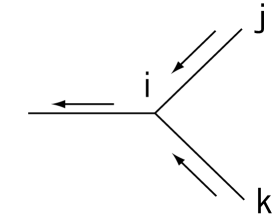
Figure 1: Local structure of a CT with coordination number $c=3$.

Let us denote the partition function in the absence of $i$’s ascendants as $Z_{i}$. Equations (9)–(12) imply that the partition function is updated as

$$Z_{i}=\sum_{S_{i},S_{j},S_{k}}Z_{j}Z_{k}\exp\{-\beta(\Delta H_{ij}+\Delta H_{ik})\}\rho_{j}(S_{j},h_{j})\rho_{k}(S_{k},h_{k}),$$ (16)

where

$$\rho_{j}(S_{j})=\frac{\exp(\beta h_{j}S_{j})}{2\cosh\beta h_{j}},$$ (17)

is the one-site marginal in the absence of $j$’s ascendants and $\Delta H_{ij}=-J_{ij}S_{i}S_{j}$ is the bond Hamiltonian added by a propagation procedure.

As a final step, the contribution from the origin of the tree is calculated as

$$Z=Z_{1}Z_{2}Z_{3}\prod_{i=1}^{3}(2\cosh\beta J_{i})$$ (18)

$$\times\left(\frac{1+\tanh\beta J_{1}\tanh\beta J_{2}\tanh\beta h_{1}\tanh\beta h_{2}+({\rm two\,\,terms\,\,with\,\,1,2,3\,\,rotated})}{4}\right),$$ (19)

and the whole partition function $Z$ is derived. Taking the $T\rightarrow 0$ limit yields the ground-state energy for a given bond configuration. In this limit, eqs. (11) and (16) become

$${\widehat{h}}_{j}\rightarrow{\rm sgn}({J_{ij}h_{j}})\min(|J_{ij}|,|h_{j}|),$$ (20)

and

$$\lim_{\beta\rightarrow\infty}-\frac{1}{\beta}\log Z_{i}=E_{i}$$ (21)

$$=E_{j}+E_{k}-J_{ij}-J_{ik}+\left\{\begin{array}[]{ll}0&\,\,(\,\,{\rm sgn}({J_{ij}J_{ik}h_{j}h_{k}})\geq 0\,\,)\\ 2\min(|J_{ij}|,|J_{ik}|,|h_{j}|,|h_{k}|)&\,\,(\,\,{\rm otherwise}\,\,)\end{array}\right..$$ (24)

We assume ${\rm sgn}({0})\equiv 0$ in this paper.

2.2.2 Use of the replica method

For a given single sample of interactions and boundary conditions, a simple application of the BP algorithm enables us to evaluate the partition function in a feasible computational time. Unfortunately, this does not fully resolve the problem of the computational cost for assessing the moments (4) since the cost for evaluating an average over all possible samples of interactions and boundary conditions grows exponentially with respect to the number of spins. However, this difficulty can be overcome by analytically assessing the configurational average for $n\in\mathbb{N}$ and analytically continuing the obtained expressions to $n\in\mathbb{C}$ in the level of the algorithm, a method which may be considered a generalization of the replica method.

For this purpose, we first evaluate the $n$th moment of the partition function $Z$

$$\Xi(n)\equiv[Z^{n}]=\Tr{}\prod_{\left\langle{i,j}\right\rangle}[\exp(\beta J_{ij}\sum_{\alpha}^{n}S^{\alpha}_{i}S^{\alpha}_{j})],$$ (25)

for $n\in\mathbb{N}$, where $\alpha$ is the replica index. Let us denote the effective Hamiltonian as

$$H_{{\rm eff}}=\sum_{\left\langle{i,j}\right\rangle}H_{ij}=\sum_{\left\langle{i,j}\right\rangle}-\frac{1}{\beta}\log[\exp(\beta J_{ij}\sum_{\alpha}S_{i}^{\alpha}S_{j}^{\alpha})],$$ (26)

where $[\cdots]$ stands for the configurational average with respect to the interactions $\{J_{ij}\}$. This means that eq. (25) is simply the partition function of an $n$-replicated system, which is defined on a cycle free graph and is free from quenched randomness. Therefore, by expressing the BP algorithm in the current case as

$$\Xi_{i}(n)=\sum_{{\mbox{\boldmath$S$}}_{i},{\mbox{\boldmath$S$}}_{j},{\mbox{\boldmath$S$}}_{k}}\left[\exp\left\{\beta(J_{ij}\sum_{\alpha}^{n}S^{\alpha}_{i}S^{\alpha}_{j}+J_{ik}\sum_{\alpha}^{n}S^{\alpha}_{i}S^{\alpha}_{k})\right\}\right]\rho_{j}\rho_{k}\Xi_{j}(n)\Xi_{k}(n)$$ (27)

$$=\sum_{{\mbox{\boldmath$S$}}_{i}}\rho_{i}({\mbox{\boldmath$S$}}_{i})\Xi_{i}(n),$$ (28)

where $\rho_{i}$ is the one-site marginal distribution of site $i$, eq. (25) can be assessed in a feasible time. The expressions (27) and (28) define the updating rules of $\rho_{i}$ and $\Xi_{i}(n)$.

So far, we have made no assumptions or approximations and therefore eq. (28) yields exact assessments for $n\in\mathbb{N}$, given a boundary condition. To generalize this scheme to $n\in\mathbb{C}$, we here introduce the RS ansatz, which is the second step of the replica method and, in general, is expressed by a restriction of the functional form of $\rho_{i}({\mbox{\boldmath$S$}}_{i})$ as

$$\rho_{i}({\mbox{\boldmath$S$}}_{i})=\int\pi_{i}(h)\prod_{\alpha=1}^{n}\left(\frac{1+\tanh(\beta h)S^{\alpha}_{i}}{2}\right)dh=\int\pi_{i}(h)\frac{e^{\beta h\sum_{\alpha}S^{\alpha}_{i}}}{(2\cosh\beta h)^{n}}dh,$$ (29)

where $\pi_{i}(h)$ is a distribution to be updated in the algorithm. The expression of eq. (29) guarantees that $\rho_{i}({\mbox{\boldmath$S$}}_{i})$ is invariant under any permutation of the replica indices $\alpha=1,2,\ldots,n$. Note that this property is automatically satisfied over all of the objective lattice if only the distributions on the boundary are expressed in the form of eq. (29).

Inserting eq. (29) into eq. (28) and performing some simple algebraic steps gives

$$\Xi_{i}=\sum_{{\mbox{\boldmath$S$}}_{i}}\Xi_{j}\Xi_{k}(2\cosh\beta)^{2n}\int dh_{i}\frac{e^{\beta h_{i}\sum_{\alpha}S^{\alpha}_{i}}}{(2\cosh\beta h_{i})^{n}}\Bigg{\{}\int\!\!\!\int\pi_{j}(h_{j})\pi_{k}(h_{k})$$ (30)

$$\times\left[\delta(h_{i}-{\widehat{h}}_{j}-{\widehat{h}}_{k})\left(\frac{2\cosh\beta h_{i}}{2\cosh\beta{\widehat{h}}_{j}2\cosh\beta{\widehat{h}}_{k}}\right)^{n}\right]dh_{j}dh_{k}\Bigg{\}}$$ (31)

$$=\sum_{{\mbox{\boldmath$S$}}_{i}}\int dh_{i}\pi_{i}(h_{i})\frac{e^{\beta h_{i}\sum_{\alpha}S^{\alpha}_{i}}}{(2\cosh\beta h_{i})^{n}}\Xi_{i}.$$ (32)

Equations (31) and (32) provide an expression of the replica symmetric BP algorithm:

$$\pi_{i}(h_{i})\propto\int\!\!\!\int\pi_{j}(h_{j})\pi_{k}(h_{k})\left[\delta(h_{i}-{\widehat{h}}_{j}-{\widehat{h}}_{k})\left(\frac{2\cosh\beta h_{i}}{2\cosh\beta{\widehat{h}}_{j}2\cosh\beta{\widehat{h}}_{k}}\right)^{n}\right]dh_{j}dh_{k},$$ (33)

$$\Xi_{i}=\Xi_{j}\Xi_{k}(2\cosh\beta)^{2n}\int\!\!\!\int dh_{j}dh_{k}\,\pi_{j}(h_{j})\pi_{k}(h_{k})\left[\left(\frac{2\cosh\beta(\widehat{h}_{j}+\widehat{h}_{k})}{2\cosh\beta{\widehat{h}}_{j}2\cosh\beta{\widehat{h}}_{k}}\right)^{n}\right],$$ (34)

which is applicable to $\forall{n}\in\mathbb{C}$. When the algorithm reaches the origin of the CT, the moment of eq. (25) is assessed as

$$\Xi(n)=[Z^{n}]=\Xi_{1}\Xi_{2}\Xi_{3}(2\cosh\beta)^{3n}\int\!\!\!\int\!\!\!\int dh_{1}dh_{2}dh_{3}\,\pi_{1}(h_{1})\pi_{2}(h_{2})\pi_{3}(h_{3})$$ (35)

$$\times\left[\left(\frac{1+\tanh\beta J_{1}\tanh\beta J_{2}\tanh\beta h_{1}\tanh\beta h_{2}+R}{4}\right)^{n}\right],$$ (36)

where $R$ is two terms with the indices $1,2,3$ rotated.

2.2.3 Zero-temperature limit

Under appropriate boundary conditions, the zero-temperature limit $\beta\to\infty$, $n\to 0$ keeping $y=\beta n$ finite, which we focus on in the present paper, yields further simplified expressions of the BP algorithm. For this, we generate replicated spins of each site on the boundary with an identical random external field $h_{i}=\pm 1$, the sign of which is determined with an equal probability of $1/2$. This yields the cavity field distribution

$$\pi_{i}(h_{i})=\frac{1}{2}\left(\delta(h_{i}-1)+\delta(h_{i}+1)\right)$$ (37)

and the partition function

$$\Xi_{i}=(2\cosh\beta)^{n}\to e^{y},$$ (38)

as the boundary condition. The relevance of the boundary condition to the current objective systems is discussed later.

Equation (37) in conjunction with the property $|J_{ij}|=1$ allows $\pi_{i}(h_{i})$ in eq. (33) to be expressed without loss of generality as

$$\pi_{i}(h_{i})=p_{i;0}\delta(h_{i})+\sum_{f=1}^{c-1}p_{i;f}\left(\delta(h_{i}-f)+\delta(h_{i}+f)\right),$$ (39)

where ${\mbox{\boldmath$p$}}_{i}=(p_{i;0},p_{i;1},\ldots,p_{i;c-1})$ represents a probability vector satisfying $p_{i;0}+2\sum_{f=1}^{c-1}p_{i;f}=1$ and $p_{i;f}\geq 0$ $(f=0,1,\ldots,c-1)$, and is to be determined from the descendent distributions. It is noteworthy that the symmetry $\rho_{i}({\mbox{\boldmath$S$}}_{i})=\rho_{i}(-{\mbox{\boldmath$S$}}_{i})$ on the boundary condition also restricts $\pi_{i}(h_{i})$ to a symmetric function of the form of eq. (39).

After the configurational average is performed, the cavity-field distribution $\pi_{i}(h_{i})$ depends only on the distance, $g$, from the boundary. Therefore, we hereafter denote $\pi_{i}(h_{i})$ as $\pi_{g}(h_{i})$ and represent the distance of the origin from the boundary as $g=L$. The BP scheme assesses ${\mbox{\boldmath$p$}}_{g+1}$ using its descendents ${\mbox{\boldmath$p$}}_{g}$. However, the only part relevant to the assessment of $\Xi(n)$ is that for $p_{g;0}$, which is represented as

$$p_{g+1;0}=\frac{p_{g;0}^{2}+2\left(\frac{1-p_{g;0}}{2}\right)^{2}e^{-2y}}{1-2(1-e^{-2y})\left(\frac{1-p_{g;0}}{2}\right)^{2}},$$ (40)

for the $c=3$ case, being accompanied by an update of the partition function

$$\Xi_{g+1}=\Xi_{g}^{2}e^{2y}\left\{1-2(1-e^{-2y})\left(\frac{1-p_{g;0}}{2}\right)^{2}\right\},$$ (41)

and similarly for a general $c$. After evaluating $p_{g;0}$ and $\Xi_{g}$ using this algorithm up to $g=L-1$, the full partition function, $\Xi(y)$, in the current limit $n\to 0$ and $\beta\to\infty$ keeping $y=n\beta\sim O(1)$ is finally assessed as

$$\Xi(y)=\Xi_{L}=\Xi_{L-1}^{3}e^{3y}\left\{1-3(1-e^{-2y})\left(\frac{1-p_{L-1;0}}{2}\right)^{2}(1+p_{L-1;0})\right\}.$$ (42)

For $\forall{y}\in\mathbb{C}$, eqs. (40)–(42) can be performed in a feasible computational time and therefore offer a useful scheme for examining RZs. This is the main result of the present paper. The concrete procedure to obtain RZs is summarized as follows:

1. To obtain a series of $p_{g;0}$, eq. (40) is recursively applied under the initial condition $p_{0;0}=0$ until $g$ reaches $L-1$. This can be symbolically performed by using computer algebra systems such as Mathematica.

2. Using the series $\{p_{g;0}\}$, the moment $\Xi_{g}$ is recursively calculated by using eq. (41) under the initial condition (38) until $g$ becomes $L-1$. Then, the full moment $\Xi(y)=\Xi_{L}$ is derived from eq. (42) using $\Xi_{L-1}$ and $p_{L-1;0}$.

3. Solving $\Xi_{L}=0$ with respect to $x=e^{y}$ numerically.

Although the right hand side of eq. (40) is expressed as a rational function, $\Xi_{L}$ and $\Xi(y)$ are guaranteed to be certain polynomials of $x$ since the contribution from the denominator is canceled in each step of eqs. (41) and (42). The procedure of (i), (ii) and (iii) can be performed in a polynomial time with respect to the number of spins. However, for CTs the number of spins and the degree of the polynomial $\Xi_{L}$ increase exponentially as $O\left(((k-1)(c-1))^{L}\right)$ as $L$ becomes larger, which makes it infeasible to solve $\Xi_{L}=0$ for large $L$. For instance, it is computationally difficult to evaluate RZs beyond $L=7$ for $(k,c)=(2,3)$ and $L=4$ for $(k,c)=(3,4)$ by use of today’s computers of reasonable performance. This prevents us from accurately examining the convergence of RZs to the real axis in the limit $L\to\infty$ by means of numerical methods and analytical investigation for this purpose is non-trivial either. However, the data of small $L$ still strongly indicate that the qualitative behavior of RZs can be classified distinctly depending on whether certain bifurcations, which are irrelevant to any RSB, occur for the cavity field distribution in the limit of $L\to\infty$. This implies that RZs of the ladder and tree systems are related to no RSB. In the following sections, we give detailed discussions to lead this conclusion presenting plots of RZs.

2.3 Remarks

Before proceeding further, there are several issues to be noted.

2.3.1 Uniqueness of the analytical continuation

As already mentioned, analytical continuation from $n\in\mathbb{N}$ to $n\in\mathbb{C}$ cannot be determined uniquely in general systems. However, in the present system, we can show the uniqueness of the continuation. Therefore, the RS solution assumed above is correct.

For this, let us consider the modified moment $[(Ze^{-\beta N_{B}})^{n}]^{1/N}$, where $N_{B}$ is the total number of bonds. This quantity satisfies the inequality

$$\left|\left[\left(Ze^{-\beta N_{B}}\right)^{n}\right]^{1/N}\right|\leq\left[\left(Ze^{-\beta N_{B}}\right)^{{\rm Re}(n)}\right]^{1/N}$$ (43)

$$\leq\left[\left(\Tr{}1\right)^{{\rm Re}(n)}\right]^{1/N}=2^{{\rm Re}(n)}<O(e^{\pi|n|}),$$ (44)

for finite $N$. Suppose that we have an analytic function $\psi(n;N)$ that satisfies the condition $|\psi(n;N)|<O(e^{\pi|n|})$. Carlson’s theorem guarantees that if the equality $|\psi(n;N)-[(Ze^{-\beta N_{B}})^{n}]^{1/N}|=0$ holds for $\forall{n}\in\mathbb{N}$, $\psi(n;N)$ is identical to $[(Ze^{-\beta N_{B}})^{n}]^{1/N}$ for $\forall{n}\in\mathbb{C}$. Because $e^{-\beta N_{B}}$ is a non-vanishing constant, this means that the analytic continuation of $[Z^{n}]^{1/N}$ is uniquely determined. This indicates that expressions analytically continued under the RS ansatz, namely eqs. (36) and (42), are correct for finite $N$ (or equivalently, finite $L$) although the analyticity may be broken on the real axis in the limit $N\to\infty$.

2.3.2 Relationship to other systems

In addition to examining RZs for finite CTs and ladder systems, the relevance of RZs to the large system size limit will also be argued by comparison with known thermodynamic properties of relatives of CTs, namely Bethe lattices and regular random graphs. These are sometimes identified with CTs because the fixed point condition of the BP method is represented identically. However, we here strictly distinguish them. The definitions and properties of these systems are summarized as follows:

• The Cayley tree (CT): A tree of finite size consisting of an origin and its neighbors. The first generation is built from $c$ neighbors which are connected to the origin. Each site in the $n$th generation is connected to new $c-1$ sites without overlap and all these new sites comprise the $n+1$th generation. Iterating this procedure to the $L$th generation, we obtain the CT, and the $L$th generation becomes its boundary. For the boundary condition of eq. (37), which implies $p_{0;0}=0$ in the expression of eq. (40), $\Xi(n)$ of this lattice is represented as a polynomial of $x=e^{-y}$, which can be assessed by symbolic operations using eqs. (40)–(42) without evaluating the values of $\Xi(n)$. This property is very useful for investigating RZs.

• The Bethe lattice (BL): A lattice consisting of the first $L^{\prime}$ generations of a CT, for which $L\to\infty$ is taken. Alternatively, we can define a BL as a finite CT of $L^{\prime}$ generation, the boundary condition of which is given by the convergent cavity field distribution of the infinite CT. Unlike for a CT, the boundary condition depends on $y$ for a BL. Due to this difference, $\Xi(n)$ of this lattice cannot be represented as a polynomial and searching RZs becomes non-trivial. However, assessing the values of $\Xi(n)$ is still feasible computationally.

• The regular random graph (RRG): A randomly generated graph under the constraint of a fixed connectivity $c$. Since there exist many cycles, assessing $\Xi(n)$ and RZs for this lattice is not feasible computationally for finite $N$. In the limit $N\to\infty$ under appropriate conditions, however, it is considered that the RRG and the BL share many identical properties. Therefore, this lattice is sometimes identified with the BL and regarded as a solvable system [25, 26, 27, 28]. Nevertheless, we here distinguish between the two systems because the main purpose of this paper is to clarify the asymptotic properties of $g_{N}(n)$ from finite $N$ to infinite $N$, and our definition of the BL is useful to compare these limits. Here, the terminology “RRG” is used only to refer to systems of infinite size.

2.3.3 Relevance of the boundary condition to the moment of the partition function

The above mentioned distinction between the three relatives of CTs yields differences in the expression of the moment of the partition function, even while they share an identical cavity field distribution in the limit $N\to\infty$.

Equations (40)–(42) imply that $g_{N}(y)=N^{-1}\log\Xi(y)$ for CTs is generally expressed as

$$g_{N}(y)=\frac{1}{N}\sum_{\left\langle ij\right\rangle}g_{\left\langle ij\right\rangle}^{(2)}(y)-\frac{1}{N}\sum_{i}(c_{i}-1)g_{i}^{(1)}(y)+\frac{1}{N}\sum_{\mu}g_{\mu}(y),$$ (45)

where $g_{\left\langle ij\right\rangle}^{(2)}(y)$ and $g_{i}^{(1)}(y)$ denote the contributions from the bond $\left\langle ij\right\rangle$ and the site $i$, respectively, and $c_{i}$ is the number of bonds that site $i$ has. The last term $g_{\mu}(y)$ is the contribution due to the boundary fields.

This is considered a generalization of a well-known property of free energies for cycle free graphs [29, 30, 31]. For regular CTs, $c_{i}=c$ holds if $i$ is placed inside the tree, while $c_{i}=1$ for the boundary sites.

For a BL, the boundary condition given by the convergent solution of eq. (40), $p_{*}$, which becomes a function of $y$, particularly simplifies the expression of eq. (45) as

$$g_{N}^{\rm BL}(y)=r_{\rm I}g_{\rm I}(y)+r_{\rm B}g_{\rm B}(y).$$ (46)

Here, $r_{\rm I}=\left(1+c(c-2)^{-1}\left((c-1)^{L^{\prime}-1}-1\right)\right)/\left(1+c(c-2)^{-1}\left((c-1)^{L^{\prime}}-1\right)\right)$ and $r_{\rm B}=1-r_{\rm I}$ represent the fractions of the number of sites inside the tree and on the boundary, respectively, and

$$g_{\rm I}(y)=\frac{c}{2}g^{(2)}(y)-(c-1)g^{(1)}(y),$$ (47)

and

$$g_{\rm B}(y)=\frac{c}{2}g^{(2)}(y)+g_{\mu}(y),$$ (48)

represent contributions from a single site inside the tree and on the boundary. In general, $g^{(2)}(y)$ and $g^{(1)}(y)$ are expressed as

$$g^{(2)}(y)=\log\left\{\Tr{}\left[\widehat{\rho}({\mbox{\boldmath$S$}}_{1})^{c-1}\widehat{\rho}({\mbox{\boldmath$S$}}_{2})^{c-1}e^{\beta J\sum_{\alpha}S_{1}^{\alpha}S_{2}^{\alpha}}\right]\right\},$$ (49)

$$g^{(1)}(y)=\log\left\{\Tr{}\widehat{\rho}({\mbox{\boldmath$S$}})^{c}\right\},$$ (50)

where

$$\widehat{\rho}({\mbox{\boldmath$S$}})=\int d\widehat{h}\widehat{\pi}(\widehat{h})\frac{e^{\beta\widehat{h}\sum_{\alpha}S_{\alpha}}}{(2\cosh\beta\widehat{h})^{n}}$$ (51)

and $\widehat{\pi}(\widehat{h})$ is the distribution of the cavity bias, which is related to $\pi(h)$ as

$$\widehat{\pi}(\widehat{h})=\int dh\pi(h)\left[\delta\left(\widehat{h}-\frac{1}{\beta}\tanh^{-1}(\tanh\beta J\tanh\beta h)\right)\right].$$ (52)

For $c=3$ in the limit $\beta n\to y$, we have

$$g^{(2)}(y)=\log e^{y}\left(1-\frac{1}{2}(1-e^{-2y})(1-p_{*})^{2}\right)^{3},$$ (53)

$$g^{(1)}(y)=\log\left(1-\frac{3}{4}(1-e^{-2y})(1-p_{*})^{2}(1+p_{*})\right),$$ (54)

$$g_{\mu}(y)=g_{0}-\log\left(1-\frac{1}{2}(1-e^{-2y})(1-p_{*})^{2}\right),$$ (55)

where $g_{0}=\log\int dhP(h)(2\cosh\beta h)^{n}$ is the contribution from a boundary spin and $P(h)$ is the boundary-field distribution of the BL determined satisfying the condition $\pi(0)=P(0)/(\int P(h)(2\cosh\beta h)^{n})=p_{*}$.

Equation (46) represents a distinctive feature of cycle free graphs. In most systems, the contribution from the boundary becomes negligible as the system size $N$ tends to infinity. However, eq. (46) indicates that such a contribution does not vanish for a BL since $r_{\rm B}\to(c-2)/(c-1)$ remains of the order of unity even if $N=1+c(c-2)^{-1}\left((c-1)^{L^{\prime}}-1\right)$ becomes infinite. Nevertheless, the complete separation of contributions between the inside and the boundary in this equation implies that it is physically plausible to use $g_{\rm I}(y)$, instead of $g_{N}^{\rm BL}(y)$, in handling problems concerning the bulk part of the objective graph. Actually, such a replacement has been adopted in several studies on cycle free graphs [26, 32]. In general, $g_{\rm I}(y)$ agree with $g(y)$ of an RRG, which provides the basis of the correspondence between BLs and RRGs.

In spin-glass problems on cycle free graphs, the replacement of $g_{N}^{\rm BL}(y)$ with $g_{\rm I}(y)$ is crucial. To see this, we here investigate the large deviation properties of $[Z^{n}]$. We denote the boundary condition as $P_{\rm B}({\mbox{\boldmath$h$}})=\prod_{i\in{\rm boundary}}\pi_{i}(h_{i})$. Equation (6) implies that $\Xi(y)$ is expressed as $\Xi(y)=\int d{\mbox{\boldmath$h$}}P_{\rm B}({\mbox{\boldmath$h$}})\exp\left(-yE_{g}({\mbox{\boldmath$h$}})\right)$, where $E_{g}({\mbox{\boldmath$h$}})$ is the ground state energy when $h$ is imposed on the boundary. For general systems, including a BL, this yields the identity

$$y^{2}(\partial/\partial y)\left(y^{-1}g_{N}(y)\right)=N^{-1}D(\widetilde{P}_{\rm B}|P_{\rm B})\geq 0,$$ (56)

where $\widetilde{P}_{\rm B}({\mbox{\boldmath$h$}})=P_{\rm B}({\mbox{\boldmath$h$}})\exp\left(-yE_{g}({\mbox{\boldmath$h$}})\right)/\Xi(y)$ and $D(\widetilde{P}_{\rm B}|P_{\rm B})$ is the Kullback–Leibler (KL) divergence between $\widetilde{P}_{\rm B}({\mbox{\boldmath$h$}})$ and ${P}_{\rm B}({\mbox{\boldmath$h$}})$. An implication of this relation from large deviation statistics is that the probability $P(f)$ that $E_{g}({\mbox{\boldmath$h$}})/N$ equals $f$ scales as $P(f)\simeq\exp\left(N\Sigma_{N}(f)\right)$ for large $N$, where $f$ and $\Sigma_{N}(f)$ are related by $f=-(\partial/\partial y)g_{N}(y)$ and $\Sigma_{N}(f)=-y^{2}(\partial/\partial y)\left(y^{-1}g_{N}(y)\right)$ parameterized by $y$. The non-negativity of the KL divergence indicates that the rate function $\Sigma_{N}(f)$ cannot be positive, which guarantees the normalization constraint $\int dfP(f)=1$.

The constraint $\Sigma_{N}(f)\leq 0$ is always satisfied even when $N\to\infty$. However, this is not necessarily the case when we take the thermodynamic limit $\lim_{N\rightarrow\infty}g_{N}(y)=g(y)$ and then calculate the rate function as $\Sigma(y)=-y^{2}(\partial/\partial y)\left(y^{-1}g(y)\right)$. This function $\Sigma(f)$ can be positive, and it can be shown that the condition $\Sigma(f_{s})=0$ signals the onset of $1$RSB [12, 33]. The positive part of $\Sigma(f)$ can be formally interpreted as the complexity or the configurational entropy of the metastable states for a single typical sample of couplings in the conventional 1RSB framework [34], as shown in fig. 2. In the 1RSB framework, the critical condition $\Sigma(f_{s})=0$, which is alternatively expressed as $(\partial/\partial y)\left(y^{-1}g(y)\right)|_{y=y_{s}}=0$ in general, corresponds to the typical state realized in equilibrium.

The condition $\Sigma(f_{s})=0$ has already been investigated for RRGs and indicates that 1RSB transitions occur for some types of RRGs [26, 28]. However, it is considered that such a symmetry breaking cannot be detected by an investigation based on eqs. (40)–(42) because the boundary contribution is inevitably taken into account for a BL as well as for a CT. Actually, direct verification of $\Sigma(f)\leq 0$ is possible for the $c=3$ case; details are shown in C. This indicates that the possible RZs provided by the current scheme are irrelevant to 1RSB.

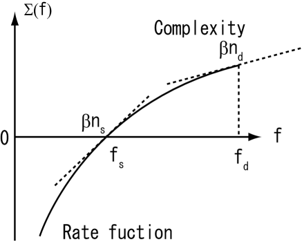
Figure 2: Schematic diagram of $\Sigma(f)$ assessed using $g_{\rm I}(y)$. The rate function is continued to the complexity at $f=f_{s}$ and the 1RSB occurs at this point. The complexity vanishes at $f=f_{d}$ where the monotonicity of the free energy with respect to $y=\beta n$ breaks down.

3 Results

3.1 Plots of the replica zeros for tree systems

We here present the results only for CTs. RZs plots for ladder systems are summarized in A.

Figure 3: Plot of RZs for a CT with $c=3$. All the zeros lie on the line ${\rm Im}(y)=\pi/2$, as for a $2\times L$ ladder. Figure 4: RZs plot for a $3$-CT with $c=3$. A sequence of zeros approaches the real axis as the number of generations $L$ increases. The arrow indicates the collision point expected from the study of the $L\to\infty$ limit in sec. 3.2.

The plots for a CT and for a $3$-CT with $c=3$ are shown in figs. 4 and 4, respectively. Note that 1RSB occurs in RRGs with the same parameters. The critical values are $y_{s}=0.41741$ and $\infty$ for the RRG counterparts of a CT and $3$-CT with $c=3$, respectively.

Figure 4 shows that RZs of the $c=3$ CT lie on a line ${\rm Im}(y)=\pi/2$. Interestingly, this behavior is the same as the $2\times L$ ladder case, the plot of which is given in A. This result indicates that there is no phase transition or breaking of analyticity of $g(n)$ with respect to real $y$. This is in accordance with the argument on the boundary contribution mentioned in the previous section.

On the other hand, for the $3$-CT case in fig. 4, a sequence of RZs approaches a point $y_{c}$ on the real axis from the line ${\rm Im}(y)=\pi/2$ as the number of generations $L$ increases, although the value of $y_{c}$ is far from $y_{s}=\infty$. A similar tendency is also observed for a CT and $3$-CT with $c=4$, plots of which are presented in figs. 6 and 6, respectively. The 1RSB critical values are $y_{s}=0.38926$ for the CT and $y_{s}=1.41152$ for the 3-CT. Again, these values are far from the values of $y_{c}$, which can be observed in figs. 6 and 6.

Figure 5: RZs of a CT with $c=4$. We consider only an $L$-generation branch in this case because of computational limits. RZs approach the real axis as $L$ increases around $y_{c}\approx 0.5$. The arrow indicates the location of the singularity of the cavity-field distribution. Figure 6: RZs of a $3$-CT with $c=4$. We consider only an $L$-generation branch. The zeros approach the real axis around $y_{c}\approx 1.1$. There are two singular points of the cavity field distribution in this case, both of which are indicated by arrows.

These results indicate that certain phase transitions occur for some CTs, although they are irrelevant to 1RSB. It is difficult to identify the critical value $y_{c}$ from the plots because of the computational limits. Instead, in the following subsection we investigate the $L\to\infty$ limit of these models. The arrows in figs. 4–6 represent the transition points $y_{c}$ determined by this investigation.

3.2 Phase transition on the boundary of a BL

In order to identify the value of $y_{c}$, we take the limit $L\to\infty$ by equating $p_{g+1;0}$ and $p_{g;0}$ in the iterative equation of $p_{g;0}$, which yields the boundary condition $p_{*}$ of the BL. For a $c=3$ 3-CT, the iterative equation is given by

$$p_{g+1;0}=\frac{\left\{p_{g;0}^{2}+2p_{g;0}(1-p_{g;0})\right\}^{2}+\frac{1}{2}e^{-2y}(1-p_{g;0})^{4}}{1-\frac{1}{2}(1-p_{g;0})^{4}(1-e^{-2y})}.$$ (57)

A return map of the recursion of $p_{g;0}$ and the convergent solution $p_{*}$ are presented in figs. 8 and 8, respectively. The return map shows that there are three fixed points for $x\$$\stackrel{{\scriptstyle\textstyle>}}{{\sim}}$$\,\ 2.35$, while $p=1$ is the only fixed point for $x\$$\stackrel{{\scriptstyle\textstyle<}}{{\sim}}$$\,\ 2.35$. This situation is in contrast to the $c=3$ CT case, in which the cavity-field distribution uniformly converges to an analytic function:

$$p_{*}=\frac{2+x^{2}-\sqrt{x^{4}+8x^{2}}}{2(1-x^{2})},$$ (58)

which can be derived from eq. (40). This implies that when eq. (37) is put on the boundary of the CT, the boundary condition of the BL, which was obtained by an infinite number of recursions $L-L^{\prime}\to\infty$, exhibits a discontinuous transition from $p_{*}<1$ to $p_{*}=1$ at $x\approx 2.35\Leftrightarrow y_{c}\approx 0.85$ as $y$ is reduced from the above. Actually, in fig. 4, RZs of the $c=3$ 3-CT seem to approach $y_{c}\approx 0.85$, marked by an arrow. This indicates that RZs obtained by our framework are relevant to the phase transition of the boundary of a BL, which is not related to 1RSB.

Figure 7: Return map of a $3$-CT with $c=3$. The convergent point of the recursion discontinuously changes depending on $x$. The solid line represents the function $f(p)=p$. Figure 8: Asymptotic behavior of $p_{g;0}$ of a $3$-CT with $c=3$. A finite jump of $p$ occurs at $x\approx 2.35$. The solid line denotes the $\L\to\infty$ solution $p_{*}$.

The same analysis for a $c=4$ CT shows that bifurcation of another type can occur for even $c$. For this model, the recursive equation of $p_{g;0}$ has a trivial solution $p_{*}=0$ for $\forall{x}$, which is always the case when $c-1$ is odd. The return map and plots of $p_{*}$ are shown in figs. 10 and 10, respectively.

Figure 9: Return map of a CT with $c=4$. The stable fixed point is unique but shows a singularity at $x=e^{y}=\sqrt{3}$. Figure 10: Asymptotic behavior of $p_{g;0}$ of a CT with $c=4$. In the thermodynamic limit, $p_{g;0}$ is continuous but the derivative becomes discontinuous at $x=\sqrt{3}$.

These figures indicate that there exists a continuous transition from $p_{*}=0$ to $p_{*}>0$ at a certain value of $x$, which can be assessed as $x_{c}=\sqrt{3}\Rightarrow y_{c}\approx 0.5$. This is consistent with a certain sequence of RZs approaching the real axis around $y_{c}\approx 0.5$ in fig. 6, which supports the analytical assessment of the critical points.

In general, the discontinuous transition appears for cases of $k\geq 3$ spin interactions and the continuous transition occurs when $c$ is even. Actually, for a $c=4$ 3-CT, both discontinuous and continuous transitions occur at $x\approx 0.86\Rightarrow y\approx-0.15$ and $x=3\Rightarrow y\approx 1.1$, respectively. Figure 6 shows a sequence of RZs approaching $y\approx 1.1$, while it is difficult to clearly identify a sequence converging to the other critical point $y\approx-0.15$. We consider that this is because the system size is not large enough, since a portion of the RZs in the left shows a tendency to approach the real axis, though further increase of the system size is practically unfeasible due to the limitations of current computational resources.

In conclusion, the analysis shown in this section indicates that RZs of CTs are related to the phase transitions on the boundary of a BL. Regardless of the type of transition, a sequence of RZs approaches a critical point on the real axis when the BL provided from a CT in the limit $L\to\infty$ exhibits a phase transition on the boundary.

4 Discussion

4.1 Possible link to AT instability

The AT condition, which is critical for FRSB, has not yet been characterized for sparsely connected spin models. In fact, previous research has found that critical values of the continuous transitions from $p_{*}=0$ to $p_{*}>0$ are candidates for those of the AT condition for systems of even $c$ [28]. This motivates us to further explore a possible link between RZs and the AT instability.

Divergence of the spin-glass susceptibility of the root site $0$ is often adopted as the critical condition of the AT instability for BLs [35, 36, 37, 38]. Generalizing the condition to the case of finite $n$, we obtain

$$\chi_{SG}=\sum_{i}\left[\left(\frac{\partial\left\langle{S_{0}}\right\rangle}{\partial h_{i}}\right)^{2}\right]_{n}.$$ (59)

where $\left[(\cdots)\right]_{n}$ means an average with respect to a modified distribution of coupling and boundary field

$$P_{n}(\{J_{ij}\},\{h_{i}\})=\frac{P(\{J_{ij}\},\{h_{i}\})Z^{n}(\{J_{ij}\},\{h_{i}\})}{\sum_{\{J_{ij}\}}P(\{J_{ij}\},\{h_{i}\})Z^{n}(\{J_{ij}\},\{h_{i}\})}.$$ (60)

This definition is reasonable because eq. (59) correctly reproduces the AT condition of fully connected systems for finite $n$ in the limit of infinite connectivity $c\to\infty$ [33, 39].

In a cycle-free graph, an arbitrary pair of nodes is connected by a single path. Let us assign node indices from the origin of the graph $0$ to a node of distance $G$ along the path as $g=1,2,\ldots,G$. For a fixed set of couplings and boundary fields, the chain rule of the derivative operation indicates that

$$\frac{\partial\left\langle{S_{0}}\right\rangle}{\partial h_{G}} = \frac{\partial\left\langle{S_{0}}\right\rangle}{\partial h_{0}}\frac{\partial h_{0}}{\partial\widehat{h}_{0}}\frac{\partial\widehat{h}_{0}}{\partial{h}_{1}}\cdots\frac{\partial h_{G}}{\partial\widehat{h}_{G}}=\frac{\partial\left\langle{S_{0}}\right\rangle}{\partial h_{0}}\frac{\partial h_{0}}{\partial\widehat{h}_{0}}\prod_{g=1}^{G}\frac{\partial\widehat{h}_{g-1}}{\partial h_{g}}\frac{\partial{h}_{g}}{\partial\widehat{h}_{g}}$$ (61)

$$= \frac{\partial\left\langle{S_{0}}\right\rangle}{\partial\widehat{h}_{0}}\prod_{g=1}^{G}\frac{\partial\widehat{h}_{g-1}}{\partial\widehat{h}_{g}},$$ (62)

as $h_{g}$ depends linearly on $\widehat{h}_{g}$ as $h_{g}=\widehat{h}_{g}+r_{g}$, where $r_{g}$ represents a sum of the cavity biases from other branches that flow into node $g$. For a BL of $(k,c)=(2,3)$, the BP update yields an evolution equation of the cavity bias

$$\widehat{h}_{g-1}=\frac{1}{\beta}\tanh^{-1}\left(\tanh(\beta J_{g})\tanh(\beta(\widehat{h}_{g}+r_{g}))\right)$$ (63)

$$\to\left\{\begin{array}[]{ll}{\rm sgn}\left(J_{g}(\widehat{h}_{g}+r_{g})\right)&(\,\,|\widehat{h}_{g}+r_{g}|\geq 1\,\,)\cr J_{g}(\widehat{h}_{g}+r_{g})&(\,\,\mbox{otherwise}\,\,)\end{array}\right.(\,\,\beta\to\infty\,\,),$$ (66)

where $J_{g}$ denotes the coupling between nodes $g-1$ and $g$, and similarly for other cases.

To assess eq. (59), we take an average of the square of eq. (66) with respect to the modified distribution $P_{n}(\{J_{ij}\},\{h_{i}\})$. Here, $r_{g}$ can be regarded as a sample of a stationary distribution determined by the convergent solution of eq. (40) for the BL. As $r_{g}$ is limited to being an integer and $|J_{g}|=1$, eq. (66) gives

$$\left|\frac{\partial\widehat{h}_{g-1}}{\partial\widehat{h}_{g}}\right|=\left\{\begin{array}[]{ll}0&(\,\,|\widehat{h}_{g}+r_{g}|>1\,\,)\\ 0\mbox{ or $1$}&(\,\,|\widehat{h}_{g}+r_{g}|=1\,\,)\\ 1&(\,\,{\rm otherwise}\,\,)\end{array}\right.,$$ (70)

where the value of $0$ or $1$ for the case of $|\widehat{h}_{g}+r_{g}|=1$ is determined depending on the value of $\widehat{h}_{g}$. When $\widehat{h}_{g}=0$ (and $|r_{g}|=1$), the values $0$ and $1$ are chosen with equal probability $1/2$ since the sign of the infinitesimal fluctuation of $\widehat{h}_{g}$, $\delta\widehat{h}_{g}$, is determined in an unbiased manner due to the mirror symmetry of the distribution of couplings. On the other hand, under the condition of $\prod_{k=g+1}^{G}\left|\partial\widehat{h}_{k-1}/\partial\widehat{h}_{k}\right|\neq 0$, the case of $|\widehat{h}_{g}|=1$ (and $r_{g}=0$) always yields $\left|\partial\widehat{h}_{g-1}/\partial\widehat{h}_{g}\right|=1$. This is because $\widehat{h}_{g}\delta\widehat{h}_{g}<0$ is guaranteed for $|\widehat{h}_{g}|=1$ under this condition.

Equation (70) indicates that the assessment of eq. (62) is analogous to an analysis of a random-walk which is bounded by absorbing walls. We denote by $P_{(G\to 0)}$ the probability that $\left|\partial\widehat{h}_{g-1}/\partial\widehat{h}_{g}\right|$ never vanishes during the walk from $G$ to $0$ and the value of $\prod_{g=1}^{G}|\partial\widehat{h}_{g-1}/\partial\widehat{h}_{g}|$ is kept to unity. This indicates that

$$\left[\left(\frac{\partial\left\langle{S_{0}}\right\rangle}{\partial h_{G}}\right)^{2}\right]_{n}\propto P_{(G\to 0)}$$ (71)

holds. Summing all contributions up to the boundary of the BL yields the expression

$$\chi_{SG}\propto\sum_{G=0}^{L^{\prime}}(k-1)^{G}(c-1)^{G}P_{(G\rightarrow 0)}.$$ (72)

The critical condition for convergence of eq. (72) in the limit $L^{\prime}\to\infty$ is

$$\log\left((k-1)(c-1)\right)+\lim_{G\to\infty}\frac{1}{G}\log P_{(G\rightarrow 0)}=0.$$ (73)

This serves as the “AT” condition in the current framework.

For a BL, eq. (73) can be assessed by analyzing the random walk problem of eq. (70), as shown in D. We evaluated the critical $y_{AT}$ values of eq. (73) for several pairs of $(k,c)$, shown in Table 1 along with other critical values.

$(k,c)$	$y_{AT}$	$y_{c}$	$y_{s}$
$(2,3)$	0.54397	none	0.41741
$(2,4)$	0.89588	$\log\sqrt{3}\approx 0.54931$	$0.38926$
$(3,3)$	1.51641	0.85545	$\infty$
$(3,4)$	1.35403	$-$0.15082, $\log 3\approx 1.09861$	1.41152

Table 1: Relevant values of $y$. Note that each kind of $y$ is calculated using different models. The 1RSB transition point $y_{s}$ is for RRGs and $y_{AT}$ is for RRGs or BLs. The singularity of the cavity-field distribution $y_{c}$ is common for all the models.

These results show that the values of $y_{c}$, which signal the phase transitions of the boundary condition of the BL, agree with neither $y_{AT}$ or $y_{s}$, implying irrelevance of RZs to the replica symmetry breaking.

The irrelevance of RZs to the AT instability may be interpreted as follows. We can link the spin-glass susceptibility to $g_{N}(n)$ in general by considering the following extension:

$$N{\widetilde{g}}_{N}({\mbox{\boldmath$F$}};m,n)=$$ (74)

$$\log\left[\left(\Tr{}\exp\left(-\beta\sum_{a=1}^{m}H({S^{a}})+\sum_{l=1}^{N}F_{l}\sum_{a<b}S_{l}^{a}S_{l}^{b}\right)\right)\left(\Tr{}e^{-\beta H}\right)^{n-m}\right],$$ (75)

by breaking the replica symmetry introducing replica symmetric interactions among $m$ out of $n$ replica systems with coupling ${\mbox{\boldmath$F$}}=(F_{1},F_{2},\ldots,F_{N})$. Obviously, $g_{N}(n)={\widetilde{g}}_{N}({\mbox{\boldmath$F$}}=0;m,n)$ and $g_{N}(n)={\widetilde{g}}_{N}({\mbox{\boldmath$F$}};m=1,n)$ hold. Analytically continuing eq. (75) to $n,m\in\mathbb{R}$ and expanding the obtained expression around ${\mbox{\boldmath$F$}}=0$ for $m\simeq 1$ yields

$$N{\widetilde{g}}_{N}({\mbox{\boldmath$F$}};m,n)\approx Ng_{N}(n)+\frac{m-1}{2}{\mbox{\boldmath$F$}}^{T}\widehat{\chi}_{SG}{\mbox{\boldmath$F$}}+({\rm higher\,\,orders}),$$ (76)

where $\widehat{\chi}_{SG}=\left(\left[\left(\left\langle{S_{l}S_{k}}\right\rangle-\left\langle{S_{l}}\right\rangle\left\langle{S_{k}}\right\rangle\right)^{2}\right]_{n}\right)$ represents the spin-glass susceptibility matrix.

Equation (76) implies that the divergence of the spin-glass susceptibility is linked to analytical singularities of $\lim_{N\to\infty}{\widetilde{g}}_{N}({\mbox{\boldmath$F$}};m,n)$ for $m\neq 1$. However, for $m=1$, which corresponds to $g_{N}(n)$ examined in the present paper, it is difficult to detect the singularity because the factor $m-1$ with ${\mbox{\boldmath$F$}}^{T}\widehat{\chi}_{SG}{\mbox{\boldmath$F$}}$ makes the divergence of the spin-glass susceptibility irrelevant to the analyticity breaking of $g(n)=\lim_{N\to\infty}g_{N}(n)$. A possible solution is to consider systems of $m\neq 1$ in the framework of 1RSB. However, an examination along this direction is beyond the scope of the present paper.

4.2 Physical implications of the obtained solutions

We concluded that bifurcations of the fixed point solutions of the BP update correspond to phase transitions of the boundary condition of a BL and are not relevant to either 1RSB or FRSB. Before closing this section, we discuss the physical implications of the obtained solutions.

A naive consideration finds that the solution of $p_{\infty;0}=p=1$ corresponds to a paramagnetic phase implying that any cavity fields vanish and therefore all spin configurations are equally generated. Note that this phase is of the ground states in the limit $\beta\rightarrow\infty$ and is different from the usual temperature-induced phase.

For finite $p<1$, relevant fractions of the spins can take any direction without energy cost because the cavity field on the site is $0$. This implies that the ground state energy is highly degenerate, which means that this solution describes a RS spin-glass phase. Actually, it is easy to confirm that the following equality holds:

$$q_{\mu\nu}=\frac{[\Tr{}S^{\mu}_{g}S^{\nu}_{g}e^{-\beta\sum_{\mu}H^{\mu}}]}{[Z^{n}]}=\Tr{}S^{\mu}_{g}S^{\nu}_{g}\rho_{g}({\mbox{\boldmath$S$}})=1-p_{g;0}.$$ (77)

Hence, the singularity of the cavity-field distribution in the limit $g\rightarrow\infty$ can be regarded as the transition of the spin-glass order-parameter. A finite jump of $\pi_{\infty}(h)$ for the $k=3$ case is the first-order transition from the RS spin glass to paramagnetic phases, and such a transition is also observed in the mean-field models. The transitions from $p=0$ to finite-$p$ for the $c=4$ case can be regarded as a saturation of $q$ to $q_{EA}=1$. We infer that these are the transitions from RS to RS phases. Notice that such a transition has not been observed for infinite-range models. Our results indicate that this $q=1$ phase appears only when $c$ is even. This means that such a phase is highly sensitive to the geometry of the objective lattice. This may be a reason why such a transition has not been observed in other models.

5 Summary

In summary, we have investigated RZs for CTs and ladders in the limit $T,n\rightarrow 0,\,\,\beta n\rightarrow y\sim O(1)$. Most of the zeros exist near the line ${\rm Im}(y)=\pi/2$ in all cases investigated; in particular, for the $(k,c)=(2,3)$ CT and the width-$2$ ladder all the zeros lie on this line. For the width-$2$ ladder we have proved that the free energy is analytic with respect to $y$ in this model. On the other hand, for some CTs, a relevant fraction of the RZs spreads away from the line ${\rm Im}(y)=\pi/2$ and approaches the real axis as the generation number $L$ grows. This implies that $g(n)$ has a singularity at a finite real $y$ in the thermodynamic limit. A naive observation finds that the RZs collision points correspond to phase transitions of the boundary condition of the BL. We have compared them with known critical conditions of 1RSB and FRSB and concluded that these conditions are irrelevant to the behavior of RZs. This is consistent with the absence of RSB in CTs reported in some earlier studies.

To fully understand and use the replica method, as well as mathematical verification, an description of the physical significance of the method is required. We hope that our results presented in this paper lead to a deeper understanding of the mysteries of the replica method.

Appendix A Results for ladder systems

We first explain the procedure to obtain the RZs of ladder systems. For a $2\times L$ ladder system, the BP equation can be derived in a similar manner to the CT case.

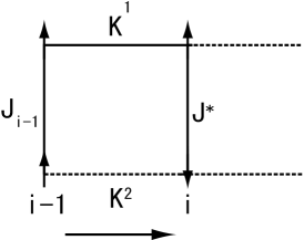
Figure 11: Unit cell of a $2\times L$ ladder.

We trace out the two spins of the previous generation to the $i$th generation, as in fig. 11. This yields an expression corresponding to eq. (9) as

$$\sum_{S_{i-1}^{1,2}}\exp\{\beta(J_{i-1}S_{i-1}^{1}S_{i-1}^{2}+K^{1}S_{i-1}^{1}S_{i}^{1}+K^{2}S_{i-1}^{2}S_{i}^{2}+J^{*}S_{i}^{1}S_{i}^{2})\}$$ (78)

$$=A\exp(\beta(J^{*}+\widehat{J}_{i-1})S_{i}^{1}S_{i}^{2}).$$ (79)

From simple algebra we obtain

$$\widehat{J}_{i-1}=\frac{1}{\beta}\tanh^{-1}(\tanh\beta K^{1}\tanh\beta K^{2}\tanh\beta J_{i-1}),$$ (80)

$$A=4\frac{\cosh\beta J_{i-1}\cosh\beta K^{1}\cosh\beta K^{2}}{\cosh\beta\widehat{J}_{i-1}}.$$ (81)

This shows that the effective bond $J_{i}$ between $S_{i}^{1}$ and $S_{i}^{2}$ becomes

$$J_{i}=J^{*}+\widehat{J}_{i-1}.$$ (82)

These relations indicate that the one-site marginal distribution $\rho_{i}$ for trees is replaced by the two-site marginal distribution $\rho_{i}(S_{i}^{1},S_{i}^{2})$ for a width-$2$ ladder. From the symmetries of the original model, we can specify the form of this distribution as

$$\rho({\mbox{\boldmath$S$}}_{i}^{1},{\mbox{\boldmath$S$}}_{i}^{2})=\int dJ_{i}\pi(J_{i})\frac{e^{\beta J_{i}\sum_{\alpha}S_{i}^{1,\alpha}S_{i}^{2,\alpha}}}{(4\cosh\beta J_{i})^{n}}.$$ (83)

This expression can be interpreted as showing that the effective bond fluctuates by quenched randomness. In a similar way to the tree case, the iterative equation for $\pi(J)$ is derived as

$$\pi_{i}(J_{I})\propto\int dJ_{i-1}\pi_{i-1}(J_{i-1})\left[\delta(J_{i}-J^{*}-\widehat{J}_{i-1})\left(\frac{\cosh\beta J_{i}}{\cosh\beta\widehat{J}_{i-1}}\right)^{n}\right],$$ (84)

and that for the effective partition function is

$$\Xi_{i}(n)=\Xi_{i-1}(n)$$ (85)

$$\times\int dJ_{i-1}\pi_{i-1}(J_{i-1})\left[(2\cosh\beta K^{1})^{n}(2\cosh\beta K^{2})^{n}\left(\frac{\cosh\beta J_{i}}{\cosh\beta\widehat{J}_{i-1}}\right)^{n}\right].$$ (86)

In the limit $\beta\rightarrow\infty,\beta n\rightarrow y$, we can derive the following formulas from above equations:

$$p_{g+1;0}=\frac{1-p_{g;0}}{1-p_{g;0}-(1+p_{g;0})e^{2y}},$$ (87)

$$\Xi_{g+1}=\Xi_{g}e^{3y}\left(p_{g;0}+\frac{1}{2}(1-e^{-2y})(1-p_{g;0})\right).$$ (88)

Using these relations, we can symbolically calculate the $\Xi_{L}$ as a polynomial of $x=e^{y}$ and obtain the RZs by numerically solving $\Xi_{L}=0$ as the CT cases.

On the other hand, for larger-width ladders, the number of spins added by an iteration is greater than $2$ and many-body interactions appear. It makes the problem complicated and simple relations like (82) cannot be obtained. Hence, when treating larger-width ladders, we directly use the BP formula for a given sample $\{J_{ij}\}$ to obtain the ground state energy [40] and numerically assess the distribution of the ground state energies $P(E_{g})$ by enumerating all the configurations. Using the distribution $P(E_{g})$, the RZs equation is derived as

$$\sum_{E_{g}}P(E_{g})e^{-yE_{g}}=0.$$ (89)

This equation is solved numerically in the same way as the other cases. Note that computational times required in the counting process to obtain $P(E_{g})$ exponentially increases as $L$ grows, which makes it infeasible to obtain $\Xi_{L}$ for large $L$.

Next, we present the plots of RZs for ladder systems with brief discussions.

Figure 12: RZs for ladders with $2\times L$. All the zeros lie on ${\rm Im}(y)=\pi/2$ and never reach the real axis of $y=\beta n$. The inequality ${\rm Re}(y)\leq\log 2\sqrt{2}$ holds, as shown in B. Figure 13: Zeros of width-$4$ ladders. Some of the zeros approach the real axis around ${\rm Re}(y)\approx 1.2$, but the rate of approach rapidly decreases as $L$ grows.

Figure 13 shows the plot for a $2\times L$ ladder with the boundary condition $p_{0;0}=0$ and $\Xi_{0}=x$. Notice that all RZs lie on a line ${\rm Im}(y)=\pi/2$. This fact can be mathematically proven, as detailed in B. The physical significance of this behavior is that the generating function $g_{N}(n)$ is analytic with respect to real $y$ even for the $N\rightarrow\infty$ limit. We have also investigated a $3\times L$ ladder and found qualitatively similar results as for the width-2 case. For a width-$4$ ladder, the RZ plot is given in fig. 13. We can observe that some zeros approach the real axis around ${\rm Re}(y)\approx 1.2$, but the rate of approach decreases rapidly as $L$ grows. This implies that the RZs do not reach the real axis, which agrees with a naive speculation that ladders are essentially one-dimensional systems and therefore do not involve any phase transitions as long as the width is kept finite.

Appendix B Location of replica zeros of a width-$2$ ladder

We prove that all RZs of a $2\times L$ ladder lie on the line ${\rm Im}(y)=\pi/2$ for any $L$. We introduce the notation

$$p_{l}(x)=p_{l;0}=\frac{n_{l}(x)}{d_{l}(x)},$$ (90)

where $d_{l}$ and $n_{l}$ are polynomials of $x=e^{y}$ and $n_{l}(x)/d_{l}(x)$ is assumed to be irreducible. The outline of the proof is as follows. First we present the general solution of $p_{l}$ and show that the denominator $d_{l}$ has $2F((l+1)/2)$ roots which are all purely imaginary. The function $F(l)$ is the floor function, which is defined to return the maximum integer $i$ in the range $i\leq l$. Also, we show that the number of nontrivial solutions of $\Xi_{l}=0$ is equal to $2F((l+1)/2)$ and $\Xi_{l}$ can be factorized as $C_{l}(x)d_{l}(x)$, where $C_{l}(x)$ is a polynomial of $x$. From the correspondence of the numbers of the roots, we conclude that all the zeros of $\Xi_{l}$ are equivalent to the roots of $d_{l}(x)$ and $C_{l}(x)$ takes the form $ax^{b}$.

The iteration (87) for $p_{l}$ has a solvable form and its general solution is given by

$$p_{l}=\frac{2(4^{l}-h(x)^{l})}{4^{l}(2+x^{2}-x\sqrt{x^{2}+8})-(2+x^{2}+x\sqrt{x^{2}+8})h(x)^{l}},$$ (91)

where

$$h(x)\equiv-4-x(x+\sqrt{x^{2}+8})=4\frac{x+\sqrt{x^{2}+8}}{x-\sqrt{x^{2}+8}}.$$ (92)

The roots of the numerator in eq. (91) can be easily calculated as

$$x=\left\{\begin{array}[]{cc}\pm 2\sqrt{2}i\hskip 56.9055pt(l=2m+1)\\ 0,\pm 2\sqrt{2}i\hskip 56.9055pt(l=2m)\end{array}\right.,$$ (93)

where $i$ denotes the imaginary unit and $m$ is a natural number. Then, we concentrate on finding the roots of the denominator in eq. (91) except for those of the numerator (93). From numerical observations in sec. 3, we found that any of the roots $x^{*}$, which satisfy $\Xi_{l}(x^{*})=0$, are purely imaginary and bounded by $|x^{*}|\leq 2\sqrt{2}$. Hence, we assume these conditions and perform the variable transformation $z=-xi$. Equating the denominator of eq. (91) to $0$, we get

$$\left(\frac{h(-ix)}{4}\right)^{l}=\left(\frac{\sqrt{8-z^{2}}+iz}{\sqrt{8-z^{2}}-iz}\right)^{l}=\frac{2-z^{2}-i\sqrt{8-z^{2}}}{2-z^{2}+i\sqrt{8-z^{2}}}.$$ (94)

We now enumerate the number of solutions under conditions that $z$ is real and bounded as $-2\sqrt{2}\leq z\leq 2\sqrt{2}$. Under these conditions, we can transform eq. (94) into a simple form by using the polar representation. The result is

$$e^{i(2\theta_{1}-\pi)l}=e^{i2\theta_{2}},$$ (95)

where $\sqrt{8-z^{2}}+iz=r_{1}e^{i\theta_{1}}\,\,(-\pi<\theta_{1}\leq\pi)$ and $r_{2}e^{i\theta_{2}}=2-z^{2}-i\sqrt{8-z^{2}}\,\,(-\pi<\theta_{2}\leq\pi)$. While $z$ varies from $-2\sqrt{2}$ to $2\sqrt{2}$ continuously, the radius $r_{1}$ stays at a constant $2\sqrt{2}$ and the argument $\theta_{1}$ varies from $-\pi/2$ to $\pi/2$ in the positive direction. In the same situation, $\theta_{2}$ changes from $+\pi$ to $-\pi$ in the negative direction. The radius $r_{2}$ is not constant, but is finite in this range. The variables $\theta_{1}$ and $\theta_{2}$ are obviously continuous and monotonic functions of $z$. Therefore, the argument of the left-hand side of eq. (95) starts from $\theta=0$ and rotates with angle $2l\pi$ in the positive direction and the counterpart of the right-hand side varies from the same point $\theta=0$ to $-4\pi$. This means that there are $l+1$ values of $z$ where the factor $(2\theta_{1}(z)-\pi)l$ becomes equal to $2\theta_{2}(z)$ except for trivial solutions $z=\pm 2\sqrt{2}$. When $l$ is even, these solutions contain a trivial solution $z=0$, which can also be confirmed from eq. (91). Hence, the number of nontrivial roots of $d_{l}$ becomes $l+1$ for odd $l$ and $l$ for even $l$, which is equivalent to $2F((l+1)/2)$.

As already noted, the number of nontrivial solutions of $\Xi_{l}=0$ is equal to $2F((l+1)/2)$. This can be understood by considering that the number of terms of $[Z^{n}]$ is determined by the maximum number of defects $n_{d}$. In the $2\times l$ ladder case, the value of $n_{d}$ is given by $F((l+1)/2)$ and the number of terms is $n_{d}+1$. The highest degree of the relevant polynomials for RZs comes from the difference between the highest and lowest ground-state energies and is given by $2n_{d}=2F((l+1)/2)$, which yields the number of nontrivial solutions of $\Xi_{l}=0$.

Finally, we prove that $\Xi_{l}$ takes the form $A_{l}x^{b_{l}}d_{l}(x)$ by induction. From eqs. (87) and (88) with the initial conditions $p_{0;0}=0,\,\,\Xi_{0}=x$, we derive

$$p_{1}=\frac{1}{x^{2}+1},\,\,\Xi_{1}=\frac{1}{2}x^{2}(x^{2}+1),$$ (96)

which satisfies the desired form. Assuming that the condition $\Xi_{l}=Ax^{b_{l}}d_{l}(x)$ is true for $l=k$, we substitute this expression into eq. (88) to get

$$\Xi_{k+1}=Ax^{b_{k}}d_{k}x^{3}\left\{\frac{n_{k}}{d_{k}}+\frac{1}{2}\left(1+\frac{1}{x^{2}}\right)\left(1-\frac{n_{k}}{d_{k}}\right)\right\}$$ (97)

$$=\frac{1}{2}Ax^{b_{k}+1}\left\{(x^{2}-1)n_{k}+(1+x^{2})d_{k}\right\}.$$ (98)

Equation (87) can be written as

$$p_{k+1}=\frac{d_{k}-n_{k}}{(x^{2}-1)n_{k}+(1+x^{2})d_{k}}=\frac{n_{k+1}}{d_{k+1}},$$ (99)

which gives

$$(x^{2}-1)n_{k}+(1+x^{2})d_{k}=c_{k+1}(x)d_{k+1}(x),$$ (100)

where $c_{k+1}$ is a polynomial and satisfies $c_{k+1}=(d_{k}-n_{k})/n_{k+1}$. Substituting this relation, we can rewrite eq. (98) as

$$\Xi_{k+1}=\frac{1}{2}Ax^{b_{k}+1}c_{k+1}(x)d_{k+1}(x).$$ (101)

As we have already shown, the number of nontrivial zeros of $\Xi_{k+1}$ is equal to that of $d_{k+1}$. This means that $c_{k+1}$ cannot have nontrivial roots and hence $c_{k+1}$ takes the form $Ax^{b}$. This completes the proof by induction and demonstrates our proposition that all RZs for a $2\times L$ ladder have a constant imaginary part $i\pi/2$.

Appendix C Rate function for a CT with $c=3$

We here calculate the generating function $g_{L}(y)$ for finite $L$. Consider an $L$-generation branch of a $c=3$ CT. An explicit form $g_{L}(y)$ is easily derived from eq. (41) as

$$g_{L}(x)=\frac{2^{L}}{2^{L+1}-1}g_{0}+\frac{2^{L+1}}{2^{L+1}-1}(1-2^{-L})\log x+\frac{1}{4-2^{-L+1}}\sum_{i=0}^{L-1}\frac{\log f_{i}}{2^{i}},$$ (102)

where $x=e^{y}$ and

$$g_{0}=\log\Xi_{0},\,\,f_{i}=f_{i}(x,p_{i;0})=1-\frac{1}{2}(1-x^{-2})(1-p_{i;0})^{2},$$ (103)

using the same notations as in sec. 2. The rate function with finite generations $L$ is given by

$$\Sigma_{L}(x)=\frac{2^{L}}{2^{L+1}-1}\left(g_{0}-x\log x\frac{dg_{0}}{dx}\right)$$ (104)

$$+\frac{1}{4-2^{-L+1}}\sum_{i=0}^{L-1}\frac{1}{2^{i}f_{i}}\left(f_{i}\log f_{i}-C_{i}(x)x\log x\right),$$ (105)

where the factor $C_{i}(x)$ is given by

$$C_{i}(x)=\frac{\partial f_{i}}{\partial p_{i;0}}\frac{dp_{i;0}}{dx}+\frac{\partial f_{i}}{\partial x}=(1-x^{-2})(1-p_{i;0})\frac{dp_{i;0}}{dx}-x^{3}(1-p_{i;0})^{2}.$$ (106)

Let us denote $\Sigma_{\infty}(x)=\lim_{L\to\infty}\Sigma_{L}(x)$. Because the inequality $\Sigma_{\infty}\leq 0$ always holds, the 1RSB transition does not occur as long as the condition $\Sigma_{\infty}(x)=\Sigma(x)$ is satisfied.

In the range $y\geq 0\Leftrightarrow 1\leq x$, the factor $f_{i}$ is bounded as $1/2\leq f_{i}\leq 1$. This guarantees the uniform convergence of $g_{L}(x)$. The boundedness of $(dp_{i;0}/dx)$ can also be shown with some calculations. These conditions guarantee that t $\Sigma_{L}(x)$ converges to a function $\Sigma_{\infty}$ uniformly. Hence, from elementary calculus, the equality $\Sigma(x)=\Sigma_{\infty}(x)$ holds, which implies the absence of 1RSB. The same conclusion is more explicitly derived for a BL because $f_{i}$ does not depend on $i$.

Appendix D AT condition for the $(k,c)=(2,3)$ case

We here evaluate the AT condition for a BL with $(k,c)=(2,3)$. To evaluate $P_{(G\rightarrow 0)}$, we construct the transition matrix of our random-walk problem. For a given $(\widehat{h}_{g},\widehat{h}_{g+1})$, the posterior distribution of $r_{g}$ is given as

$$p(r_{g}|\widehat{h}_{g})=p(r_{g},\widehat{h}_{g})/p(\widehat{h}_{g})\propto e^{y(|r_{g}+\widehat{h}_{g}|-|r_{g}|-|\widehat{h}_{g}|)}p(r_{g}),$$ (107)

where $p(r_{g})$ is the prior distribution of $r_{g}$. This enables us to derive the concrete expression of $p(r_{g}|\widehat{h}_{g})$, summarized in Table 2.

$r_{g}$ $\backslash$ $\widehat{h}_{g}$	1	0	$-1$
1	$\displaystyle\frac{1-p_{b}}{(1+p_{b})+(1-p_{b})e^{-2y}}$	$\displaystyle\frac{1-p_{b}}{2}$	$\displaystyle\frac{(1-p_{b})e^{-2y}}{(1+p_{b})+(1-p_{b})e^{-2y}}$
0	$\displaystyle\frac{2p_{b}}{(1+p_{b})+(1-p_{b})e^{-2y}}$	$\displaystyle p_{b}$	$\displaystyle\frac{2p_{b}}{(1+p_{b})+(1-p_{b})e^{-2y}}$
$-1$	$\displaystyle\frac{(1-p_{b})e^{-2y}}{(1+p_{b})+(1-p_{b})e^{-2y}}$	$\displaystyle\frac{1-p_{b}}{2}$	$\displaystyle\frac{1-p_{b}}{(1+p_{b})+(1-p_{b})e^{-2y}}$

Table 2: Values of $p(r_{g}|\widehat{h}_{g})$ for $(k,c)=(2,3)$. The symbol $p_{b}$ is the probability that the cavity bias takes the value $0$.

We can distinguish three states of the walker at the $g$-step as follows:

$|{1}\rangle$:

The walker has already vanished.

$|{2}\rangle$:

The walker survives and $|\widehat{h}_{g}|=1$.

$|{3}\rangle$:

The walker survives and $|\widehat{h}_{g}|=0$.

Hence, using the relation (70), the transition matrix $T$ can be written as

$$T=\left(\begin{array}[]{ccc}1&p_{1,1}&\frac{1}{2}p_{1,0}\times 2\\ 0&p_{0,1}&\frac{1}{2}p_{1,0}\times 2\\ 0&p_{-1,1}&p_{0,0}\end{array}\right),$$ (108)

where $p_{r_{g},\widehat{h}_{g}}$ represents $p(r_{g}|\widehat{h}_{g})$ and the condition $p_{r_{g},\widehat{h}_{g}}=p_{-r_{g},-\widehat{h}_{g}}$ applies. When $|\widehat{h}_{g}+r_{g}|=1$ and $|\widehat{h}_{g}|=0$, the states $|{1}\rangle$ and $|{2}\rangle$ occur with equal probability $1/2$, while $|{2}\rangle$ is always chosen when $|\widehat{h}_{g}+r_{g}|=1$ and $|\widehat{h}_{g}|=1$ as exlained in sec. 4.1. This matrix has three eigenvalues: $\lambda_{1}=1,\,\lambda_{2},$ and $\lambda_{3}$. The eigenvector of the largest eigenvalue $\lambda_{1}=1$ corresponds to the state $|{1}\rangle$ or the vanishing state. Hence, the surviving probability $P_{(G\rightarrow 0)}$ is given by $1-\langle{1}|{G}\rangle$, where $|{G}\rangle$ is the state of the walker at the $G$ step. For large $G$, the relevant state is of the second-largest eigenvalue $\lambda_{2}$, and we get

$$P_{(G\rightarrow 0)}\approx\lambda_{2}^{G}.$$ (109)

Using the stationary solution (58), we obtain $P_{(G\rightarrow 0)}$ as a function of $x=e^{y}$. The AT condition becomes

$$\chi_{SG}\propto\sum_{G}(k-1)^{G}(c-1)^{G}P_{(G\rightarrow 0)}\rightarrow\infty\Leftrightarrow(k-1)(c-1)\lambda_{2}>1.$$ (110)

This condition is easily examined numerically and we can verify that the AT instability occurs at $y_{AT}\approx 0.54397$ for $(k,c)=(2,3)$.

References

References

- [1] Mézard M, Parisi G and Virasoro M A 1987 Spin Glass Theory and Beyond (Singapore: World Scientific)
- [2] Sherrington D and Kirkpatrick S 1975 Phys. Rev. Lett.35 1792
- [3] Parisi G 1980 J. Phys. A: Math. Gen.73 L115
- [4] Parisi G 1980 J. Phys. A: Math. Gen.13 1101
- [5] Talagrand M 2006 Ann. Math. 163 221
- [6] Nishimori H 2001 Statistical Physics of Spin Glasses and Information Processing: An Introduction (Oxford: Oxford University Press)
- [7] Sourlas N 1989 Nature 339 693
- [8] Kabashima Y and Saad D 1999 Europhys. Lett. 45 97
- [9] Nishimori H and Wong K Y M 1999 Phys. Rev.E 60 132
- [10] Titchmarsh E C 1939 The Theory of Functions 2nd. ed. (Oxford: Oxford University Press)
- [11] van Hemmen J L and Palmer R G 1979 J. Phys. A: Math. Gen.12 563
- [12] Ogure K and Kabashima Y 2004 Prog. Theor. Phys. 111 661
- [13] Moukarzel C and Parga N 1991 Physica A 177 24
- [14] Moukarzel C and Parga N 1991 Physica A 185 305
- [15] Derrida B 1981 Phys. Rev.B 24 2613
- [16] Ogure K and Kabashima Y 2005 Prog. Theor. Phys. Supplement 157 103
- [17] Bowman D R and Levin K 1982 Phys. Rev.B 25 3438
- [18] Chayes J T, Chayes L, Sethna J P and Thouless D J 1986 Commun. Math. Phys. 106 41
- [19] Mottishaw P 1987 Europhys. Lett. 4 333
- [20] Carlson J M, Chayes J T, Chayes L, Sethna J P and Thouless D J 1998 Europhys. Lett. 5 355
- [21] Lai P and Goldschmidt Y Y 1989 J. Phys. A: Math. Gen.22 399
- [22] Parisi G and Rizzo T 2007 Large Deviations in the Free-Energy of Mean-Field Spin-Glasses Preprint arXiv:0706.1180
- [23] Fisher M E 1965 Lectures in Theoretical Physics vol. 7 (Boulder: University of Colorado Press)
- [24] Matveev V and Shrock R 1995 Phys. Rev.E 53 254
- [25] Wong K Y M and Sherrington D 1987 J. Phys. A: Math. Gen.20 L793
- [26] Mézard M and Parisi G 2001 Euro. Phys. J. B 20 217
- [27] Mézard M and Parisi G 2003 J. Stat. Phys. 111 1
- [28] Montanari A and Ricci-Tersenghi F 2003 Euro. Phys. J. B 33 339
- [29] Katsura S, Inawashiro S and Fujiki S 1979 Physica 99A 193
- [30] Nakanishi K 1980 Phys. Rev.B 23 3514
- [31] Yedidia J S, Freeman W T and Weiss Y 2005 IEEE Trans. Inform. Theory 51 2282
- [32] Mézard M and Montanari A 2006 J. Stat. Phys. 124 1317
- [33] Nakajima T and Hukushima K 2008 J. Phys. Soc. Japan77 074718
- [34] Monasson R 1995 Phys. Rev. Lett.75 2847
- [35] Thouless D J 1986 Phys. Rev. Lett.56 1082
- [36] Rivoire O, Biroli G, Martin O C and Mézard M 2004 Eur. Phys. J. B 37 55
- [37] Krzakala F, Montanari A, Ricci-Tersenghi F, Semerjian G and Zdebrova L 2007 Proc. Natl. Acad. Sci. 104 10318
- [38] Martin O C, Mézard M and Rivoire O 2005 J. Stat. Mech P09006
- [39] Gardner E 1985 Nucl. Phys.B 257 747
- [40] Kadowaki T, Nonomura Y and Nishimori H 1996 J. Phys. Soc. Japan65 1609