Scattering matrices and expansion coefficients
of Martian analogue palagonite particles

Abstract

We present measurements of ratios of elements of the scattering matrix of Martian analogue palagonite particles for scattering angles ranging from 3^∘ to 174^∘ and a wavelength of 632.8 nm. To facilitate the use of these measurements in radiative transfer calculations we have devised a method that enables us to obtain, from these measurements, a normalized synthetic scattering matrix covering the complete scattering angle range from 0^∘ to 180^∘. Our method is based on employing the coefficients of the expansions of scattering matrix elements into generalized spherical functions. The synthetic scattering matrix elements and/or the expansion coefficients obtained in this way, can be used to include multiple scattering by these irregularly shaped particles in (polarized) radiative transfer calculations, such as calculations of sunlight that is scattered in the dusty Martian atmosphere.

Proposed Running Head:
Scattering matrices of Martian analogue palagonite

Please send Editorial Correspondence to:

E.C. Laan
TNO Science & Industry
Stieltjesweg 1
2600 AD Delft, The Netherlands

Email: eriklaan@dds.nl
Phone: +31 6 47974621
Fax: +31 15 2692111

1 Introduction

Dust from the Martian surface is regularly swept up by winds to form local, regional, or sometimes even planet-wide dust storms. The airborne dust particles scatter and absorb solar radiation and are therefore very important for the thermal structure of the thin Martian atmosphere and for the temperature of the Martian surface (see e.g. Bougher et al., 2006; Gurwell et al., 2005; Smith, 2004; Gierasch and Goody, 1972, and references therein). The interaction between radiation and the dust particles thus has to be taken into account when studying, for example, the local and global climate on Mars. In particular, one has to account for the spatial distribution of the dust particles, their number density, and their optical properties. For a given wavelength, the optical properties of the dust particles depend on their composition, sizes and shapes.

Despite the important role of dust particles in the Martian atmosphere, surprisingly little is known about their optical properties (for an overview, see Korablev et al., 2005). Consequently, in radiative transfer calculations that are used to interpret space or ground-based observations of Mars, various assumptions are made regarding the dust optical properties. In particular, it is common to assume homogeneous, spherical or spheroidal dust particles (Pollack et al., 1995; Tomasko et al., 1999), although dust particles on Earth are known to be irregularly shaped. The optical properties of homogeneous, spherical particles can straightforwardly be calculated using Lorenz-Mie theory (van de Hulst, 1957; de Rooij and van der Stap, 1984), and those of homogeneous, spheroidal particles using e.g. the so-called T-matrix method (Mishchenko and Travis, 1994; Dubovik et al., 2006). The optical properties of spherical particles can, however, differ significantly from those of irregularly shaped particles, even if their composition and/or size distribution is the same. Therefore, assuming spherical instead of irregularly shaped particles in radiative transfer calculations that are used for example to analyze observations, can lead to significant errors in retrieved atmospheric parameters, such as the dust optical thickness and/or dust particle size distributions (for a discussion on such errors, see e.g. Dlugach and Petrova, 2003; Dlugach et al., 2002).

For irregularly shaped particles, which are very common in nature, the scattering matrix elements can in principle be calculated with numerical methods such as those based on the so–called Discrete Dipole Approximation (DDA) method (see e.g. Draine and Flatau, 1994). However, the vast amounts of computing time that such numerical calculations require make it at least very impractical to calculate complete scattering matrices for a sample of particles with various (irregular) shapes and various sizes, in particular if the particles are large compared to the wavelength of the scattered light. Alternatively, employing geometrical optics for unrealistically spiky particles combined with an imaginary part of the refractive index that is rather small compared to the typical values used in the literature, appears to be useful to reproduce the scattering behavior of irregularly shaped mineral particles (see Nousiainen et al., 2003). As suggested by e.g. Tomasko et al. (1999); Dlugach and Petrova (2003); Wolff and Clancy (2003), a more practical method to obtain elements of the scattering matrix for an ensemble of irregularly shaped particles is to measure the elements in a laboratory. Note that measured scattering matrix elements are also essential for validating numerical methods and approximations.

In this article, we present measurements of ratios of elements of the scattering matrix of irregularly shaped, randomly oriented Martian analogue palagonite particles, described by Banin et al. (1997), as functions of the scattering angle. The material palagonite is believed to be a reasonable, but not perfect, analogue for the Martian surface and atmospheric dust particles. Terrestrial palagonite particles (i.e. terrestrial weathering products of basaltic ash or glass) have been put forward as Martian dust analogues (Evans and Adams, 1981; Roush and Bell, 1995) because of spectral similarities observed with visible and near-infrared spectroscopic observations using both Earth-based telescopes and several Mars orbiting spacecraft (Singer, 1985; Soderblom, 1992).

The measurements have been performed using a HeNe laser, which has a wavelength of 632.8 nm, and for scattering angles, $\Theta$, ranging from 3^∘ (near-forward scattering) to 174^∘ (near-backward scattering). Other examples of such measurements for irregularly shaped mineral particles obtained with the same experimental set-up have been reported by e.g. Volten et al. (2005) and references therein. Since we have measured ratios of all (non-zero) elements of the scattering matrix as functions of the scattering angle, our results can be used for radiative transfer calculations that include multiple scattering and polarization. As described by e.g. Lacis et al. (1998), ignoring polarization, i.e. using only scattering matrix element (1,1) (the so-called phase function), in multiple scattering calculations, induces errors in calculated fluxes. The use of only the phase function should be limited to single scattering calculations for unpolarized incident light.

A practical limitation of our experimental method is that we cannot measure close ($<6^{\circ}$) to the exact backscattering direction ($\Theta=180^{\circ}$), because there our detector would interfere with the incoming beam of light, nor close ($<3^{\circ}$) to the exact forward scattering direction ($\Theta=0^{\circ}$), because there our detector would intercept the unscattered part of the incident beam. These two scattering directions are, however, important for radiative transfer applications. This holds in particular for the near-forward scattering direction, since a significant fraction of the light that is incident on a particle is generally scattered in the near-forward direction. A solution to the lack of measurements in the near-forward and near-backward scattering directions is to add artificial data points. For the near-forward scattering direction, where a strong peak in the phase function is expected, one can add artificial data points calculated using e.g. Lorenz-Mie calculations. This has been done before, e.g. by Kahnert and Nousiainen (2007); Liu et al. (2003); Veihelmann et al. (2004); Herman et al. (2005). In this article, we use a method similar to that of Liu et al. (2003), that was also used by e.g. Muñoz et al. (2007), but we extend this by using expansion coefficients which result from a Singular Value Decomposition (SVD) fit to the measurements with generalized spherical functions (Gel’fand et al., 1963; Hovenier and van der Mee, 1983; de Rooij and van der Stap, 1984; Hovenier et al., 2004). With the added artificial data points and the expansion coefficients, we construct a so–called synthetic scattering matrix, which is normalized so that the average of the synthetic phase function over all directions equals unity and covers the whole scattering angle range (i.e. from 0^∘ to 180^∘).

Tables of the measurements, the synthetic scattering matrix elements and the expansion coefficients will be available from the Amsterdam Light Scattering Database. See Volten et al. (2005, 2006) for a description of this database.

The structure of this article is as follows. In Sect. 2, we describe the microphysical properties of our Martian analogue palagonite dust particles. In Sect. 3, we define the scattering matrix, describe the experimental set-up, and present the measurements and an auxiliary scattering matrix. In Sect. 4, we introduce the expansion coefficients, describe the Singular Value Decomposition fitting method, and present the derived expansion coefficients and synthetic scattering matrix. In Sect. 5, finally, we summarize and discuss our results.

2 Martian analogue palagonite particles

Palagonite is a fine–grained weathering product of basaltic glass. At visible wavelengths it has a refractive index, $m$, typical for silicate materials, i.e. Re($m$) is about 1.5 and Im($m$) is in the range $10^{-3}$ to $10^{-4}$ (Clancy et al., 1995). Palagonite contains a considerable fraction (about 10% by mass) of iron (III) oxide (Fe₂O₃) (Roush and Bell, 1995), which gives Mars its reddish color.

The sample in this study is sample 91-16 that is described in detail by Banin et al. (1997). Note that there is another Martian analogue palagonite sample described in the literature, namely sample 91-1 (see Roush and Bell, 1995). Palagonite sample 91-1 appears to contain more sodium than sample 91-16 because of evaporation and deposition of salt due to the proximity of its retrieval site to the Pacific Ocean. Palagonite sample 91-16 was retrieved at the top of Hawaii’s Mauna Kea volcano, about 4 km above sea level, where it was formed in a semi–arid environment likely associated with ephemeral melting water from ice. Hence, sample 91-16 is considered to be the better alternative for Martian dust of the two Martian palagonite analogues.

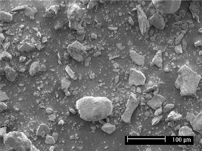
Figure 1: Scanning electron microscope (SEM) image of the Martian analogue palagonite particles used in this study. Note that SEM images generally give a good indication of the typical shapes of particles, but not necessarily of their sizes.

Before using sample 91-16 in our light scattering experiment, we removed the millimeter-sized particles by using a sieve with a 200-$\mu$m grid width, to avoid clogging the aerosol generator. Figure 1 shows an image of the palagonite particles obtained with a scanning electron microscope (SEM). This image clearly shows the irregular shapes of the palagonite particles. It should be noted that SEM images are not necessarily representative of the size distribution of the particles. The normalized projected-surface-area distribution of the dust particles was measured by using a laser particle sizer that is based on diffraction without making assumptions about the refractive indices of the materials of the particles (Konert and Vandenberghe, 1997). From the projected-surface-area distribution, we derive the number distribution and the volume distribution of the particles because these distributions are often required for numerical applications. Figure 2 shows the normalized number, volume, and projected-surface-area distributions of our Martian analogue palagonite particles as functions of $\log r$, with $r$ the radius of a projected-surface-area equivalent sphere (for details on these size distributions, see Appendix A of Volten et al., 2005). The number distribution of our palagonite particles was approximated by a log-normal distribution, yielding an effective radius, $r_{\rm eff}$, of 4.46 $\mu$m and an effective variance, $v_{\rm eff}$, of 7.29. Note that $v_{\rm eff}$ is a dimensionless parameter. For precise definitions of $r_{\rm eff}$ and $v_{\rm eff}$ see Hansen and Travis (1974), Eqs. (2.53) and (2.54), respectively.

We are well aware of the fact that the sizes of real Martian dust particles can be very different from those in our sample. Indeed, sizes of dust particles on Mars will probably vary from location to location, and from time to time, especially when in local or global storms, dust particles are lifted up from the surface to be deposited somewhere else: depending on the atmospheric turbulence, the particles in the Martian atmosphere could have very different size distributions than those on the surface.

The effective radius of 4.46 $\mu$m of our sample particles is a factor of 2 to 3 larger than the values put forward for the effective radius of Martian dust by Wolff and Clancy (2003), who analyzed observations by the Thermal Emission Spectrometer (TES) on-board the Mars Global Surveyor, and by Pollack et al. (1995), who analyzed observations performed by the Viking Lander. In particular, Pollack et al. (1995) derived an effective radius of 1.85 $\pm~{}0.3~{}\mu$m. From Pathfinder measurements, Tomasko et al. (1999) derived an effective radius of $1.6\pm 0.15$ $\mu$m. Lemmon et al. (2004) derived values from observations by the Mars Exploration Rovers Spirit and Opportunity that are similar to those of Pollack et al. (1995) and Tomasko et al. (1999).

Although our sample particles thus seem to be rather large, it should be noted that particle sizes as derived from observations will depend on the observing method, e.g. looking at diffuse skylight or at the surface, as well as on the retrieval method. In particular, according to numerical similations by Dlugach et al. (2002), effective radii that are derived for spheroidal dust particles at visibile wavelengths, under the assumption that these particles are spherical, can be significantly underestimated. At infrared wavelengths, Min et al. (2003) and Fabian et al. (2001) show that absorption and emission processes, even in the small size parameter regime (i.e. $2\pi r_{\rm eff}/\lambda\leq 1$), depend on the particle shape, too. Clearly, because Martian dust is expected to show a great variety in microphysical properties, our results should simply be regarded as an example of what can be expected for the scattering properties of irregularly shaped particles.

3 The scattering matrix

3.1 Definition of the scattering matrix

The flux and state of polarization of a quasi-monochromatic beam of light can be described by means of a so-called flux vector. If such a beam of light is scattered by an ensemble of randomly oriented particles, separated by distances larger than their linear dimensions and in the absence of multiple scattering as in our experimental set-up (see Sect. 3.2), the flux vectors of the incident beam, $\pi{\bf\Phi_{0}}(\lambda)$, and scattered beam, $\pi{\bf\Phi}(\lambda,\Theta)$, are for each scattering direction, related by a $4\times 4$ matrix, as follows (van de Hulst, 1957; Volten et al., 2006):

$${\bf\Phi}(\lambda,\Theta)=\frac{\lambda^{2}}{4\pi^{2}D^{2}}\left(\begin{array}[]{c c c c}F_{11}&F_{12}&F_{13}&F_{14}\\ F_{12}&F_{22}&F_{23}&F_{24}\\ -F_{13}&-F_{23}&F_{33}&F_{34}\\ F_{14}&F_{24}&-F_{34}&F_{44}\\ \end{array}\right){\bf\Phi_{0}}(\lambda),$$ (1)

where the first elements of the column vectors are fluxes divided by $\pi$ and the other elements describe the state of polarization of the beams by means of Stokes parameters. Furthermore, $\lambda$ is the wavelength, and $D$ is the distance between the ensemble of particles and the detector. The scattering plane, i.e. the plane containing the directions of the incident and scattered beams, is the plane of reference for the flux vectors. The matrix, ${\bf F}$, with elements $F_{ij}$ is called the scattering matrix of the ensemble. The scattering matrix elements $F_{ij}$ are dimensionless, and depend on the number of the particles and on their microphysical properties (size, shape and refractive index), the wavelength of the light, and the scattering direction. For randomly oriented particles, the scattering direction is fully described by the scattering angle $\Theta$, the angle between the directions of propagation of the incident and the scattered beams.

According to Eq. (1), a scattering matrix has in general 10 different matrix elements. For randomly oriented particles with equal amounts of particles and their mirror particles, as we can assume applies for the particles of our ensemble, the four elements $F_{13}(\Theta)$, $F_{14}(\Theta)$, $F_{23}(\Theta)$, and $F_{24}(\Theta)$ are zero over the entire scattering angle range (see van de Hulst, 1957). This leaves us only six non-zero scattering matrix elements, as follows

$${\bf F}(\Theta)=\left[\begin{array}[]{cccc}F_{11}(\Theta)&F_{12}(\Theta)&0&0\\ F_{12}(\Theta)&F_{22}(\Theta)&0&0\\ 0&0&F_{33}(\Theta)&F_{34}(\Theta)\\ 0&0&-F_{34}(\Theta)&F_{44}(\Theta)\end{array}\right],$$ (2)

where $|F_{ij}(\Theta)/F_{11}(\Theta)|\leq 1$ (Hovenier et al., 1986).

For unpolarized incident light, matrix element $F_{11}(\Theta)$ is proportional to the flux of the singly scattered light and is also called the phase function. Also, for unpolarized incident light, the ratio $-F_{12}(\Theta)/F_{11}(\Theta)$ equals the degree of linear polarization of the scattered light. The sign indicates the direction of polarization: a negative degree of polarization indicates that the scattered light is polarized parallel to the reference plane, whereas a positive degree of polarization indicates that the light is polarized perpendicular to the reference plane. In calculations for fluxes only and where light is scattered only once, $F_{11}(\Theta)$ is the only matrix element that is required. Ignoring the other matrix elements, and hence the state of polarization of the light, in multiple scattering calculations, usually leads to errors in calculated fluxes (see e.g. Lacis et al., 1998; Moreno et al., 2002; Stam and Hovenier, 2005).

3.2 The experimental set-up

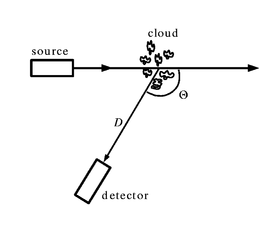
Figure 3: Sketch of the experimental set–up. The light source (a HeNe laser) emits a beam of quasi-monochromatic light, which passes through a polarizer and a modulator (not shown). The light is scattered by the ensemble of palagonite particles. A detector measures the flux that is scattered over a scattering angle $\Theta$. Measurements can be performed for $3^{\circ}\leq\Theta\leq 174^{\circ}$.

Our measurements have been performed with the light scattering experiment located in Amsterdam, the Netherlands (see e.g. Volten et al., 2005; Hovenier et al., 2003; Hovenier, 2000; Volten et al., 2001; Muñoz et al., 2000). Figure 3 shows a sketch of the experimental set–up. In our experimental apparatus, we use a HeNe laser ($\lambda$=632.8 nm, 5 mW) as a light source. The laser light passes through a polarizer and an electro-optic modulator. The modulated light is subsequently scattered by an ensemble of randomly oriented particles from the sample, located in a jet stream produced by an aerosol generator. The scattered light may pass through a quarter-wave plate and an analyzer, depending on the scattering matrix element of interest (for details see e.g. Volten et al., 2005), and is then detected by a photomultiplier tube which moves in steps along a ring with radius $D$ (see Eq. (1)) around the ensemble of particles; in this way a range of scattering angles from 3^∘ (nearly forward scattering) to 174^∘ (nearly backward scattering) is covered in the measurements.

We cannot measure close ($<3^{\circ}$) to the exact forward scattering direction, because there our detector would intercept the unscattered part of the incident beam, nor can we measure close ($<6^{\circ}$) to the exact backscattering direction, because there our detector would interfere with the incoming beam of light.

A photomultiplier placed at a fixed position (i.e. at a fixed scattering angle) is used to correct the measured scattered fluxes for time fluctuations in the particle stream. It can safely be assumed that during the measurements, the particles are in the single scattering regime (Hovenier et al., 2003).

Due to the lack of measurements between 0^∘ and 3^∘ and between 174^∘ and 180^∘, we cannot measure the absolute angular dependency of the phase function, e.g. normalized to unity when averaged over all scattering directions. Instead, we normalize the measured phase function to unity at a scattering angle of 30^∘. We present the other scattering matrix elements divided by the original measured phase function. We thus present ratios of elements of the scattering matrix instead of the elements themselves.

3.3 Measurements

Figure 4 shows the six measured not identically zero (cf. Eq. 2) ratios of elements of the scattering matrix of the Martian analogue palagonite particles as functions of the scattering angle $\Theta$, together with the experimental errors. We have verified that the measured ratios of the elements of the scattering matrix satisfy the Cloude coherency matrix test (Hovenier et al., 2004) within the experimental errors. And we verified that the other measured ratios of the elements of the scattering matrix, i.e. $F_{13}(\Theta)/F_{11}(\Theta)$, $F_{23}(\Theta)/F_{11}(\Theta)$, $F_{14}(\Theta)/F_{11}(\Theta)$, and $F_{24}(\Theta)/F_{11}(\Theta)$, do not differ from zero by more than the experimental errors (see Eq. (2)).

To illustrate the influence of the particle shape on the scattering behavior of the palagonite particles, the measurements in Fig. 4 are presented together with results of Lorenz-Mie calculations (van de Hulst, 1957; de Rooij and van der Stap, 1984) for homogeneous, optically nonactive, spherical particles at a wavelength of 632.8 nm. For the Lorenz-Mie calculations we employed the number size distribution, $n(r)$, derived from the measured projected-surface-area distribution, and the refractive index was fixed to $m=1.5+0.0005i$ (cf. Sect. 2 and Fig. 2).

As can be seen in Fig. 4, the measured phase function, i.e. $F_{11}(\Theta)/F_{11}(30^{\circ})$, of the irregularly shaped Martian analogue palagonite particles covers almost three orders of magnitude between $\Theta=3^{\circ}$ and $\Theta=174^{\circ}$, with a strong peak towards the smallest scattering angles (the so-called forward scattering peak) and a smooth drop-off towards the largest scattering angles. The measured phase function is very flat for scattering over intermediate ($70^{\circ}<\Theta<150^{\circ}$) and large ($\Theta>150^{\circ}$) scattering angles. The relatively flat appearance of the phase function of the palagonite particles at large scattering angles appears to be a general behavior for (terrestrial) irregularly shaped mineral particles with moderate refractive indices (see e.g. Volten et al., 2001; Muñoz et al., 2000, 2001). Our palagonite phase function resembles the phase functions measured in-situ with the Viking (Pollack et al., 1995) and Pathfinder missions (Tomasko et al., 1999). In Sect. 5, we make a more detailed comparison between our phase function and those presented by Tomasko et al. (1999).

As mentioned before (see Sect. 3.1), the ratio $-F_{12}(\Theta)/F_{11}(\Theta)$ represents the degree of linear polarization of the singly scattered light for incident unpolarized light. For the irregularly shaped palagonite particles, Fig. 4 shows that this ratio has a characteristic (positive) bell shape at intermediate scattering angles and a small negative branch for $\Theta\gtrsim 160^{\circ}$. For scattering angles larger than about 140^∘, the scattering angle dependence of our measured ratio $-F_{12}(\Theta)/F_{11}(\Theta)$ resembles Earth-based observations of the planetary phase angle dependence of the degree of linear polarization of Mars (Dlugach and Petrova, 2003; Shkuratov et al., 2005) (the planetary phase angle equals 180${}^{\circ}-\Theta$ for single scattering). This suggests that the polarization opposition effect that is observed at small phase angles for most solid solar system bodies (see e.g. Rosenbush and Kiselev, 2005, and references therein) can be explained, at least partly, by single scattering by small irregular particles. Here, it should be noted that the observations discussed by Dlugach and Petrova (2003) and Shkuratov et al. (2005) pertain to light that has been scattered in the Martian atmosphere combined with light that has been reflected by the surface. It is thus not purely representative for airborne dust particles.

The most striking difference between the measured and the calculated ratios $-F_{12}(\Theta)/F_{11}(\Theta)$ (Fig. 4) is their sign, hence the direction of polarization of the scattered light for unpolarized incident light. The irregularly shaped particles mostly yield scattered light polarized perpendicular to the reference plane, while the spherical particles yield scattered light polarized parallel to this plane. Another difference is that for the irregularly shaped particles, ratio $-F_{12}(\Theta)/F_{11}(\Theta)$ is a smooth, almost featureless function of $\Theta$, while for the spherical particles, the ratio shows strong angular features, especially at large scattering angles.

Scattering matrix element ratio $F_{22}(\Theta)/F_{11}(\Theta)$ is often used as a measure for the non-sphericity of the scattering particles, since for homogenous, optically inactive spheres, this ratio equals unity at all scattering angles. As can be seen in Fig. 4, for the irregularly shaped palagonite particles, $F_{22}(\Theta)/F_{11}(\Theta)$ deviates significantly from unity at all but the smallest scattering angles. Indeed, with increasing scattering angle, it decreases to slightly below 0.4 at $\Theta\approx 130^{\circ}$, and then increases again to 0.5 when $\Theta$ approaches 180^∘. The scattering angle dependence measured for the palagonite particles is similar in shape to that reported for irregularly shaped mineral aerosol particles (Volten et al., 2001), and for e.g. various types of volcanic ashes (Muñoz et al., 2004). According to Volten et al. (2001), the minimum value at intermediate scattering angles and the maximum value at the largest scattering angles are affected by the size and refractive index of the particles.

Another indication for the shape of the scattering particles are the ratios $F_{33}(\Theta)/F_{11}(\Theta)$ and $F_{44}(\Theta)/F_{11}(\Theta)$. As can also be seen in Fig. 4, for homogenous, optically inactive spheres, $F_{33}(\Theta)\equiv F_{44}(\Theta)$ (Hovenier et al., 2004), whereas we find significant differences between the measured $F_{44}(\Theta)/F_{11}(\Theta)$ and $F_{33}(\Theta)/F_{11}(\Theta)$ for the palagonite sample. The ratio $F_{33}(\Theta)/F_{11}(\Theta)$ is zero at a smaller scattering angle than $F_{44}(\Theta)/F_{11}(\Theta)$, and has a lower minimum (-0.5 versus -0.2). Indeed, for the irregularly shaped particles, these ratios show an apparently typical behavior for non-spherical particles (Mishchenko et al., 2000), namely, at large scattering angles, $F_{44}(\Theta)/F_{11}(\Theta)$ is larger than $F_{33}(\Theta)/F_{11}(\Theta)$.

Finally, scattering matrix element ratio $F_{34}(\Theta)/F_{11}(\Theta)$ of the irregularly shaped particles shows a shallow bell shape with slightly negative branches for $\Theta<30^{\circ}$ and for $\Theta>165^{\circ}$. This scattering angle dependence is commonly found for irregularly shaped silicate particles (e.g. Volten et al., 2005, 2001; Muñoz et al., 2000). Interestingly, whereas for the irregularly shaped particles, $F_{34}(\Theta)/F_{11}(\Theta)$ is very similar to $-F_{12}(\Theta)/F_{11}(\Theta)$, for the spherical particles, these ratios differ strongly from each other, both in sign and in shape, as can be seen in Fig. 4.

Comparison between the measured and the calculated scattering matrix element ratios in Fig. 4 supports the idea that scattering by non-spherical particles generally leads to smoother functions of the scattering angle than scattering by spherical particles. This smooth scattering behavior by irregularly shaped particles proves to be very difficult to simulate numerically without taking into account the irregular shape of the particles (Nousiainen et al., 2003; Nousiainen and Vermeulen, 2003; Kokhanovsky, 2003).

An electronic table of the measured ratios of the elements of the scattering matrix will be available from the Amsterdam Light Scattering Database (Volten et al., 2005, 2006).

3.4 The auxiliary scattering matrix

It appears to be difficult to directly use the measured ratios of elements of the scattering matrix in radiative transfer calculations, because of the lack of measurements below $\Theta=3^{\circ}$ and above $\Theta=174^{\circ}$. In particular, it would be interesting to have the forward scattering peak in the phase function since it contains a large fraction of the scattered energy (see Fig. 4), and is thus very important for the accurate modelling of scattered light in e.g. planetary atmospheres. In addition, the lack of measurements at small and large scattering angles inhibits the normalization of scattering matrix elements such that the average of the phase function over all scattering directions equals unity. With such a normalization and a value for the single scattering albedo of the scattering particles, one could model the absolute amount of radiation that is scattered in a given direction.

To facilitate the use of the measured ratios of elements of the scattering matrix in radiative transfer calculations, we construct from these a so–called auxiliary scattering matrix, ${\bf F^{\rm au}}$, for which holds (for $i,j=1$ to 4 with the exception of $i=j=1$),

$$F^{\rm au}_{ij}(\Theta)=\frac{F_{ij}(\Theta)}{F_{11}(\Theta)}F_{11}^{\rm au}(\Theta),$$ (3)

where the auxiliary phase function ${F_{11}^{\rm au}}$ is equal to

$$F_{11}^{\rm au}(\Theta)=\frac{F_{11}(\Theta)}{F_{11}(30^{\circ})}F_{11}^{\rm au}(30^{\circ})\hskip 28.45274pt{\rm for}\hskip 14.22636pt3^{\circ}\leq\Theta\leq 174^{\circ}.$$ (4)

This auxiliary phase function is normalized according to

$$\frac{1}{4\pi}\int_{4\pi}F^{\rm au}_{11}(\Theta)\,d\omega=1,$$ (5)

where $d\omega$ is an element of solid angle. Combining Eq. (4) and Eq. (5) and setting $F^{\rm au}_{11}(30^{\circ})$ equal to $1/C$ leads to

$$\frac{1}{4\pi}\int_{4\pi}\frac{F_{11}(\Theta)}{F_{11}(30^{\circ})}\,d\omega=C.$$ (6)

where $C$ is a normalization constant. This constant can in principle be obtained by evaluating the integral on the left-hand side of Eq.  (6), provided the function to be integrated is known over the full range of scattering angles. Therefore, we added artificial datapoints at 0 and 180 degrees to the measured values of $F_{11}(\Theta)/F_{11}(30^{\circ})$. At $\Theta=180^{\circ}$, the smoothness of the measured phase function allows us to simply add an artificial data point to $F_{11}(\Theta)/F_{11}(30^{\circ})$ by spline extrapolation (Press et al., 1992) of the measured data points.

Adding an artificial data point to the measured $F_{11}(\Theta)/F_{11}(30^{\circ})$ at $\Theta=0^{\circ}$, is more complicated. Numerical tests with the calculated phase function for the hypothetical homogeneous, spherical palagonite particles (see Fig. 4) show that extrapolation of the calculated phase function at $\Theta\leq 3^{\circ}$ towards $\Theta=0^{\circ}$, using e.g. splines (Press et al., 1992), fails to reproduce the strength of the calculated forward scattering peak. We thus decided not to extrapolate the measured phase function from $\Theta=3^{\circ}$ towards $\Theta=0^{\circ}$. Instead we add an artificial data point to the measured $F_{11}(\Theta)/F_{11}(30^{\circ})$ at $\Theta=0^{\circ}$ using the phase function that we calculated for the projected-surface-area equivalent, homogeneous, spherical particles. The rationale for this approach, which is similar to that used by Liu et al. (2003) and Muñoz et al. (2007), is that the forward scattering peak results mainly from the diffraction of the incident light. The strength of the diffraction peak and its scattering angle dependence appears to depend mainly on the size of the particles and fairly shape independent for projected-surface-area equivalent convex particles in random orientation (Mishchenko et al., 2002).

Because our normalization of the measured phase function, $F_{11}(\Theta)/F_{11}(30^{\circ})$, at $\Theta=30^{\circ}$ is rather arbitrary (we could have chosen a different value of $\Theta$ for the normalization), we scale the phase function as calculated for the spherical palagonite particles to the measured phase function. For this, we use the following equation,

$$\frac{F_{11}(0^{\circ})}{F_{11}(30^{\circ})}=\frac{F_{11}^{\rm s}(0^{\circ})}{F_{11}^{\rm s}(3^{\circ})}\frac{F_{11}(3^{\circ})}{F_{11}(30^{\circ})},$$ (7)

with $F_{11}(0^{\circ})/F_{11}(30^{\circ})$ the artificial data point at $\Theta=0^{\circ}$ and the superscript ”s” indicating the phase function as calculated for the spherical particles.

We now have data points available across the full scattering angle range to evaluate the integral in Eq. (6) and to obtain the normalization constant $C$. The numerical evaluation of this integral, however, appears to be difficult because of the steep slope between $\Theta=0^{\circ}$ and $\Theta=3^{\circ}$, where no measured data points are available. Therefore, we have chosen a different method to obtain the normalization constant $C$ in Eq. (6). This method is based on the expansion of the measured phase function $F_{11}(\Theta)/F_{11}(30^{\circ})$, including the added, artificial, data points at $\Theta=0^{\circ}$ to $\Theta=180^{\circ}$, as a function of the scattering angle into so–called generalized spherical functions (Gel’fand et al., 1963; Hovenier and van der Mee, 1983; de Rooij and van der Stap, 1984; Hovenier et al., 2004). This method of obtaining expansion coefficients from scattering matrix elements is explained in detail in Sect. 4. The expansion of $F_{11}(\Theta)/F_{11}(30^{\circ})$ yields expansion coefficients $\alpha^{l}_{1}$ (with $0\leq l$). The first of these expansion coefficients, $\alpha^{0}_{1}$, is equal to constant $C$ in Eq. (6) (Hovenier et al., 2004). Having obtained $C$ in this way, and thus $F_{11}^{\rm au}(30^{\circ})$, we readily find $F_{11}^{\rm au}(\Theta)$ from the measured ratio $F_{11}(\Theta)/F_{11}(30^{\circ})$ and Eq.  (4).

Next, given the auxiliary phase function, we derive the synthetic matrix elements $F_{ij}^{\rm au}(\Theta)$ for $i,j=1$ to 4 with the exception of $i=j=1$ from the measured ratios $F_{ij}(\Theta)/F_{11}(\Theta)$, using Eq. (3). To obtain also the complete scattering angle range for the other scattering matrix element ratios, we extrapolate the measured $F_{ij}(\Theta)/F_{11}(\Theta)$ ($i,j=1$ to 4 with the exception of $i=j=1$) towards $\Theta=0^{\circ}$ and $180^{\circ}$. At these two scattering angles, the following equalities should hold: (see Display 2.1 in Hovenier et al., 2004)

$$F_{12}(0^{\circ})/F_{11}(0^{\circ})=F_{34}(0^{\circ})/F_{11}(0^{\circ})=0,$$ (8)

$$F_{22}(0^{\circ})/F_{11}(0^{\circ})=F_{33}(0^{\circ})/F_{11}(0^{\circ}),$$ (9)

$$F_{22}(180^{\circ})/F_{11}(180^{\circ})=-F_{33}(180^{\circ})/F_{11}(180^{\circ}),$$ (10)

$$F_{12}(180^{\circ})/F_{11}(180^{\circ})=F_{34}(180^{\circ})/F_{11}(180^{\circ})=0,$$ (11)

$$F_{44}(180^{\circ})/F_{11}(180^{\circ})=1-2F_{22}(180^{\circ})/F_{11}(180^{\circ}).$$ (12)

Following Eq. (8), ratios $F_{12}(0^{\circ})/F_{11}(0^{\circ})$ and $F_{34}(0^{\circ})/F_{11}(0^{\circ})$ are set equal to zero. Following Eq. (9), we use splines to extrapolate the ratios $F_{22}(\Theta)/F_{11}(\Theta)$ and $F_{33}(\Theta)/F_{11}(\Theta)$ towards $\Theta=0^{\circ}$, and we set both $F_{22}(0^{\circ})/F_{11}(0^{\circ})$ and $F_{33}(0^{\circ})/F_{11}(0^{\circ})$ equal to the average of the two extrapolated values. Ratio $F_{44}(0^{\circ})/F_{11}(0^{\circ})$ is obtained by extrapolating (with splines) the ratio $F_{44}(\Theta)/F_{11}(\Theta)$ from $\Theta=3^{\circ}$ towards $\Theta=0^{\circ}$.

In the backward scattering direction, the measured scattering matrix element ratios $F_{ij}(\Theta)/F_{11}(\Theta)$ appear to be smooth functions of $\Theta$ (see Fig. 4). We use splines (Press et al., 1992) to extrapolate $F_{22}(\Theta)/F_{11}(\Theta)$, and $F_{33}(\Theta)/F_{11}(\Theta)$ from $\Theta=174^{\circ}$ to $\Theta=180^{\circ}$. Because $F_{22}(180^{\circ})/F_{11}(180^{\circ})$ should be equal to $-F_{33}(180^{\circ})/F_{11}(180^{\circ})$ (see Eq. (10)), we set both $F_{22}(180^{\circ})/F_{11}(180^{\circ})$ and $-F_{33}(180^{\circ})/F_{11}(180^{\circ})$ equal to the average of the two extrapolated values. Following Eq. (11), we set $F_{12}(180^{\circ})/F_{11}(180^{\circ})$ and $F_{34}(180^{\circ})/F_{11}(180^{\circ})$ equal to zero, and calculate $F_{44}(180^{\circ})/F_{11}(180^{\circ})$ using Eq. (12) with $F_{22}(180^{\circ})/F_{11}(180^{\circ})$.

In the following, we will refer to the elements of our auxiliary scattering matrix ${\bf F}^{\rm au}(\Theta)$ as (see Hovenier et al., 2004):

$${\bf F}^{\rm au}(\Theta)=\left[\begin{array}[]{cccc}a_{1}(\Theta)&b_{1}(\Theta)&0&0\\ b_{1}(\Theta)&a_{2}(\Theta)&0&0\\ 0&0&a_{3}(\Theta)&b_{2}(\Theta)\\ 0&0&-b_{2}(\Theta)&a_{4}(\Theta)\end{array}\right].$$ (13)

4 Expansion coefficients

4.1 Definitions of the expansion coefficients

For use in numerical radiative transfer algorithms, it is often advantageous to expand the elements of a scattering matrix as functions of the scattering angle into so–called generalized spherical functions (Gel’fand et al., 1963; Hovenier and van der Mee, 1983; de Rooij and van der Stap, 1984; Hovenier et al., 2004). The advantage of using the coefficients of this expansion, the so–called expansion coefficients, instead of the elements of a scattering matrix themselves is that it can significantly speed up multiple scattering calculations, which is of particular importance when polarization is taken into account (Hovenier et al., 2004; de Haan et al., 1987).

We indicate the generalized spherical functions by $P_{m,n}^{l}(\cos{\Theta})$ with the indices $m$ and $n$ equal to +2, +0, -0, or -2, and with $l\geq{\rm max}\{|m|,|n|\}$. Note that generalized spherical function $P_{0,0}^{l}$ is simply a Legendre polynomial. The expansion of the elements of auxiliary scattering matrix ${\bf F}^{\rm au}(\Theta)$ (see Eq. (13)) into generalized spherical functions is as follows:

$$a_{1}(\Theta) = \sum_{l=0}^{\infty}\alpha_{1}^{l}P_{0,0}^{l}(\cos{\Theta}),$$ (14)

$$a_{2}(\Theta)+a_{3}(\Theta) = \sum_{l=2}^{\infty}(\alpha_{2}^{l}+\alpha_{3}^{l})P_{2,2}^{l}(\cos{\Theta}),$$ (15)

$$a_{2}(\Theta)-a_{3}(\Theta) = \sum_{l=2}^{\infty}(\alpha_{2}^{l}-\alpha_{3}^{l})P_{2,-2}^{l}(\cos{\Theta}),$$ (16)

$$a_{4}(\Theta) = \sum_{l=0}^{\infty}\alpha_{4}^{l}P_{0,0}^{l}(\cos{\Theta}),$$ (17)

$$b_{1}(\Theta) = \sum_{l=2}^{\infty}\beta_{1}^{l}P_{0,2}^{l}(\cos{\Theta}),$$ (18)

$$b_{2}(\Theta) = \sum_{l=2}^{\infty}\beta_{2}^{l}P_{0,2}^{l}(\cos{\Theta}).$$ (19)

Here, $\alpha_{1}^{l}$, $\alpha_{2}^{l}$, $\alpha_{3}^{l}$, $\alpha_{4}^{l}$, $\beta_{1}^{l}$, and $\beta_{2}^{l}$ are the expansion coefficients. For each value of integer $l$, the expansion coefficients can be derived from the auxiliary scattering matrix elements using the definitions of the generalized spherical functions and their orthogonality relations (see Hovenier et al., 2004).

A similar expansion in generalized spherical functions can be made for any scattering matrix of the form given by Eq.  (2). The coefficient $\alpha^{0}_{1}$ is always equal to the average of the one-one element over all directions (Hovenier et al., 2004). So for the auxiliary phase function $a_{1}(\Theta)$ we have, according to Eq.  (5), $\alpha^{0}_{1}$ = 1 and for the measured phase function, $F_{11}(\Theta)/F_{11}(30^{\circ})$ we have $\alpha^{0}_{1}$ = C, as mentioned in Sect. 3.4.

4.2 The Singular Value Decomposition method

To derive the expansion coefficients of the measured phase function, incuding the points added at 0 and 180 degrees, and of all six elements of the auxiliary scattering matrix we write each of the Eqs. (14)–(19) into the following general form:

$$y(\Theta)=\sum_{l=n}^{m}\gamma^{l}X^{l}(\Theta),$$ (20)

where $y(\Theta)$ represents the value of the measured phase function or an auxiliary scattering matrix element at scattering angle $\Theta$, or, in the case of $a_{2}$ and $a_{3}$, respectively their sum, as in Eq. (15), or difference, as in Eq. (16). The functions $X^{l}(\Theta)$ in Eq. (20) are the basis functions, for which we choose the appropriate generalized spherical functions (Hovenier et al., 2004; de Haan et al., 1987). The parameters $\gamma^{l}$ in Eq. (20) represent the expansion coefficients, or, in the case of $\alpha_{2}^{l}$ and $\alpha_{3}^{l}$, respectively their sum (Eq. (15)) or difference (Eq. (16)). Furthermore in Eq. (20), $n$ equals 0 or 2, depending on the auxiliary scattering matrix element under consideration (see Eqs. (14)–(19)), and, although theoretically $m$ equals $\infty$ (see Eqs. (14)–(19)), in practice $m$ is restricted to the number of scattering angles at which values of the auxiliary scattering matrix elements $y(\Theta)$ are available.

For a linear model such as that represented by Eq. (20), the merit function $\chi^{2}$ is generally defined as:

$$\chi^{2}=\sum_{i=1}^{k}\left[\frac{y(\Theta_{i})-\sum_{l=n}^{m}\gamma^{l}X^{l}(\Theta_{i})}{\sigma_{i}}\right]^{2},$$ (21)

where $k$ is the number of available data points and $\sigma_{i}$ is the error associated with data point $y(\Theta_{i})$. We use the Singular Value Decomposition (SVD) method (Press et al., 1992) to solve Eq. (21) for the expansion coefficients $\gamma^{l}$, because this method is only slightly susceptible to roundoff errors and provides a solution that is the best approximation in the least-squares sense, both for overdetermined systems (in which the number of data points is larger than the required number of expansion coefficients) and underdetermined systems (in which the number of data points is smaller than the required number of expansion coefficients).

To test the robustness and the quality of the fit method based on the SVD method, we applied it to scattering matrix elements that we calculated for the hypothetical, spherical palagonite particles, and that are shown in Fig. 4 (note that our Mie-algorithm (de Rooij and van der Stap, 1984) provides matrix elements normalized according to Eq. (5), although in Fig. 4, the normalization of the elements has been adapted to correspond to that of the measurements). For the test we compare the matrix elements calculated with our Mie-algorithm with the matrix elements obtained using the expansion coefficients derived with the SVD method and Eqs. (14)-(19). For the relative errors in the matrix elements we adopt the values of the experimental errors.

We tested two aspects of the application of the SVD method. First, we applied the method to matrix elements calculated at the same set of scattering angles as the measured ratios of matrix elements, i.e. having a typical angular resolution of 5^∘ and scattering angles ranging from $3^{\circ}$ to 174^∘. Comparing the matrix elements obtained using the expansion coefficients that were derived with the SVD method with the directly calculated matrix elements, we found that the relatively coarse angular sampling and the lack of data points below $\Theta=3^{\circ}$ gave rise to strong oscillations in the matrix elements that were calculated from the derived expansion coefficients. In addition, with the derived expansion coefficients, we could not reproduce the strong forward scattering peak in the phase function. The lack of data points above $\Theta=174^{\circ}$ appeared to be less of a problem, probably because of the smoothness of the matrix elements at those scattering angles.

Second, we applied the SVD method to matrix elements calculated at an angular resolution of 1^∘ and covering the full scattering angle range, i.e. from 0^∘ to 180^∘. The matrix elements obtained using the hence derived expansion coefficients coincided within the numerical precision with the directly calculated matrix elements. From this we conclude that our implementation of the SVD method is reliable, but that we have to apply it to the whole scattering angle range, and with a relatively high angular resolution.

Finally, we found that averaging two sets of derived expansion coefficients, one of which has one coefficient more than the other, removes most of the left-over oscillations in the scattering matrix element that is calculated with the coefficients.

4.3 The derived expansion coefficients

For deriving the expansion coefficients of the scattering matrix elements of the Martian analogue palagonite particles, we use the elements of the auxiliary scattering matrix ${\bf F}^{\rm au}(\Theta)$ (see Sect. 3.4), because they cover the whole scattering angle range and are normalized according to Eq. 5.

We increase the angular sampling of the auxiliary scattering matrix by adding artificial data points by spline interpolation to the dataset between $\Theta=3^{\circ}$ and $174^{\circ}$. Starting with 44 measured data points per matrix element, adding the artificial data points results in 220 data points for each of the auxiliary scattering matrix elements. This amount of artificial data points includes the values at the forward and backward scattering angles at respectively $\Theta=0^{\circ}$ and $\Theta=180^{\circ}$ as described in Sect. 3.4. The 220 datapoints proved to be required to be able to follow the steep slopes of $a_{1}(\Theta)$, $a_{2}(\Theta)$, $a_{3}(\Theta)$ and $a_{4}(\Theta)$ between $\Theta=0^{\circ}$ and $\Theta=3^{\circ}$, where no artifical datapoints were added, without introducing unwanted oscillations. As 220 datapoints are needed to obtain the auxilliary phase function $a_{1}(\Theta)$, it proved to be practical to extend also $F_{12}(\Theta)/F_{11}(\Theta)$ and $F_{34}(\Theta)/F_{11}(\Theta)$ to the same amount of 220 datapoints, to be able to straightforwardly apply Eq. 3 to obtain $b_{1}(\Theta)$ and $b_{2}(\Theta)$.

The optimal number of expansion coefficients for each of the elements was obtained in an iterative process: unrealistic oscillations at large scattering angles are suppressed when using a smaller number of expansion coefficients, while the fit of the steep phase function near $0^{\circ}$ is improved when using a larger number of expansion coefficients. Applying our SVD method to the auxiliary scattering matrix elements, leaves us with respectively 185 expansion coefficients for $a_{1}(\Theta)$, $a_{2}(\Theta)$, $a_{3}(\Theta)$, $a_{4}(\Theta)$, 130 expansion coefficients for $b_{1}(\Theta)$ and 46 expansion coefficients for $b_{2}(\Theta)$. Figure 5 shows the expansion coefficients $\alpha^{l}_{1}$, $\alpha^{l}_{2}$, $\alpha^{l}_{3}$, $\alpha^{l}_{4}$, $\beta^{l}_{1}$, and $\beta^{l}_{2}$, derived from the auxiliary scattering matrix of the Martian analogue palagonite particles. The expansion coefficients are plotted with error bars that originate from the experimental errors in the measurements. An electronic table of the expansion coefficients will be available from the Amsterdam Light Scattering Database (Volten et al., 2005, 2006).

4.4 The synthetic scattering matrix

Employing Eqs. (14)–(19) with the expansion coefficients presented in Sect. 4.3, we can now calculate, at an arbitrary angular resolution, the so–called synthetic scattering matrix (see also Muñoz et al., 2004) which covers the complete scattering range, i.e. from 0^∘ to 180^∘, and which is normalized according to Eq. (5). Figure 6 shows the calculated synthetic scattering matrix elements. The elements of the synthetic scattering matrix are also listed in Table 1 at an angular resolution of 1 to 5 degrees. An electronic table of the synthetic scattering matrix elements will be available from the Amsterdam Light Scattering Database (Volten et al., 2005, 2006). As a check we used the synthetic scattering matrix to compute the same ratios of elements as have been measured. We found the differences to lie within the ranges of experimental uncertanties or very nearly so.

5 Summary and discussion

We present measured ratios of elements of the scattering matrix of irregularly shaped Martian analogue palagonite particles (Roush and Bell, 1995; Banin et al., 1997) as functions of the scattering angle $\Theta$ ($3^{\circ}\leq\Theta\leq 174^{\circ}$) at a wavelength of 632.8 nm. Our measured ratios of scattering matrix elements differ strongly from those calculated for homogeneous, spherical particles with the same size and refractive index. In particular, the measured phase function (ratio $F_{11}(\Theta)/F_{11}(30^{\circ})$) shows a very strong (almost three orders of magnitude) forward scattering peak and a smooth drop-off towards the largest scattering angles, where the phase function of the spherical particles shows much more angular features especially in the backward scattering direction. Clearly, using scattering matrix elements that have been calculated for homogeneous, spherical particles when irregularly shaped particles are to be expected in radiative transfer calculations for e.g. the interpretation of remote-sensing observations can thus lead to errors in retrieved dust properties (microphysical parameters and/or optical thicknesses).

To facilitate the use of our measurements in radiative transfer calculations for e.g. Mars, we have first constructed an auxiliary scattering matrix from the measured scattering matrix. This auxiliary scattering matrix covers the whole scattering angle range (i.e. from 0^∘ to 180^∘), and its elements have been normalized such that the average of the phase function over all scattering directions equals unity. The value of the phase function at $\Theta=0^{\circ}$ has been computed from the phase function calculated with Mie-theory for homogeneous, spherical particles with the same size and composition. The normalization of the auxiliary phase function, and hence the normalization of the other elements too, is obtained by applying a Singular Value Decomposition (SVD) method to fit an expansion in generalized spherical functions (Gel’fand et al., 1963; Hovenier et al., 2004) to the measured phase function, including artificial data points. The first expansion coefficient yields the required normalization constant. After the normalization of the auxiliary phase function, the SVD method is applied to the auxiliary scattering matrix and its expansion coefficients are obtained.

With the expansion coefficients, a synthetic scattering matrix is computed for the complete scattering range. It is normalized so that the average of its one-one element over all directions equals unity. The synthetic scattering matrix elements can also straightforwardly be used in radiative transfer calculations. The need to include all scattering matrix elements, instead of only the phase function, is obvious for the interpretation of polarization observations. However, even for flux calculations, all scattering matrix elements should be used, because ignoring polarization, i.e. using only the phase function, in multiple scattering calculations induces errors in calculated fluxes (e.g. Lacis et al., 1998). The use of only the phase function should be limited to single scattering calculations for unpolarized incident light.

Figure 7 shows a comparison between our synthetic phase function and two phase functions presented by Tomasko et al. (1999) as derived from diffuse skylight observations of the Imager for Mars Pathfinder. Each of the phase functions has its own normalization. The phase functions of Tomasko et al. (1999) show the same general angular behavior as our synthetic phase function: a strong forward scattering peak and a smooth drop-off towards the largest scattering angles. The forward scattering peak of our phase function appears to be stronger than the peaks of the phase functions of Tomasko et al. (1999). This can easily be due to the size difference of the particles. The dust particles in our sample have an effective radius that is a factor of 2 to 3 larger than that of Tomasko et al. (1999) (4.46 $\mu$m versus 1.6 $\mu$m $\pm$ 0.15 $\mu$m). The slopes of the phase functions in the backward scattering direction are very similar, and appear to be typical for (terrestrial) irregularly shaped mineral particles with moderate refractive indices (see e.g. Volten et al., 2001; Muñoz et al., 2000, 2001). This smooth slope can not be easily anticipated from Mie-theory.

The expansion coefficients, the synthetic scattering matrix elements, and the measured ratios of elements of the scattering matrix of the Martian analogue palagonite particles will all be available from the Amsterdam Light Scattering Database (for details, see Volten et al., 2005, 2006). The Amsterdam Light Scattering Database contains a collection of measured scattering matrix element ratios, including information on particle sizes and their composition, for various types of irregularly shaped particles. The SVD method presented in this article can straightforwardly be applied to measured scattering matrix elements of particles other than the Martian analogue palagonite particles.

Figure 2: Measured size distributions of the Martian analogue palagonite particles. The lines refer to the normalized number distribution (plusses), the normalized projected-surface-area distribution (triangles), and the normalized volume distribution (crosses) as functions of $\log r$, with $r$ the radius (in microns) of a projected-surface-area-equivalent sphere (see Volten et al., 2005, for the definitions of the various distributions). Approximating the normalized number distribution with a log normal distribution function yields $r_{\rm eff}=4.46~{}\mu$m and $v_{\rm eff}=7.29$.

Figure 4: Ratios of scattering matrix elements as functions of the scattering angle. Crosses show the ratios of elements measured, at $\lambda=632.8$ nm, for the Martian analogue palagonite particles, with the vertical bars indicating the experimental errors. Solid lines show the ratios of elements calculated using Mie-theory for homogeneous, spherical particles that are distributed in size as shown in Fig. 2.

Figure 5: The expansion coefficients $\alpha_{1}^{l}$, $\alpha_{2}^{l}$, $\alpha_{3}^{l}$, $\alpha_{4}^{l}$, $\beta_{1}^{l}$ and $\beta_{2}^{l}$ as functions of integer $l$, with their absolute errors, as derived from the auxiliary scattering matrix elements $a_{1}(\Theta)$, $a_{2}(\Theta)$, $a_{3}(\Theta)$, $a_{4}(\Theta)$, $b_{1}(\Theta)$, and $b_{2}(\Theta)$, respectively.

Figure 6: The synthetic scattering matrix elements $a_{1}$, $a_{2}$, $a_{3}$, $a_{4}$, $b_{1}$, and $b_{2}$ as functions of the scattering angle $\Theta$.

Figure 7: The synthetic phase function of the Martian analogue palagonite particles compared to the phase function derived by Tomasko et al. (1999) from Mars Pathfinder results. Each of the curves has its own normalization.

$\Theta$	$a_{1}(\Theta)$	$a_{2}(\Theta)$	$a_{3}(\Theta)$	$a_{4}(\Theta)$	$b_{1}(\Theta)$	$b_{2}(\Theta)$
0	4.36E+003	4.26E+003	4.26E+003	4.12E+003	0.00E+000	0.00E+000
1	2.82E+003	2.75E+003	2.75E+003	2.66E+003	-2.34E-003	-7.15E-003
2	6.60E+002	6.43E+002	6.43E+002	6.17E+002	1.98E-002	-2.68E-002
3	3.71E+001	3.58E+001	3.62E+001	3.49E+001	7.32E-002	-5.39E-002
4	2.51E+001	2.43E+001	2.46E+001	2.38E+001	9.69E-002	-8.20E-002
5	1.53E+001	1.46E+001	1.49E+001	1.43E+001	7.28E-002	-1.05E-001
6	1.17E+001	1.13E+001	1.14E+001	1.10E+001	4.88E-002	-1.18E-001
7	8.75E+000	8.44E+000	8.49E+000	8.18E+000	3.73E-002	-1.20E-001
8	7.08E+000	6.82E+000	6.82E+000	6.60E+000	1.66E-002	-1.12E-001
9	5.68E+000	5.48E+000	5.48E+000	5.29E+000	-1.68E-003	-9.83E-002
10	4.80E+000	4.62E+000	4.61E+000	4.42E+000	-1.55E-003	-8.22E-002
15	2.35E+000	2.22E+000	2.21E+000	2.12E+000	-4.94E-003	-4.04E-002
20	1.42E+000	1.32E+000	1.31E+000	1.23E+000	-8.44E-003	-2.15E-002
25	9.68E-001	8.93E-001	8.80E-001	8.13E-001	-9.63E-003	-1.35E-002
30	6.98E-001	6.27E-001	6.18E-001	5.60E-001	-1.05E-002	-3.85E-003
35	5.22E-001	4.57E-001	4.47E-001	4.08E-001	-1.15E-002	2.72E-003
40	4.06E-001	3.44E-001	3.32E-001	3.00E-001	-1.30E-002	8.12E-003
45	3.24E-001	2.68E-001	2.50E-001	2.25E-001	-1.46E-002	9.34E-003
50	2.68E-001	2.13E-001	1.96E-001	1.75E-001	-1.55E-002	1.23E-002
55	2.24E-001	1.71E-001	1.52E-001	1.38E-001	-1.66E-002	1.46E-002
60	1.90E-001	1.37E-001	1.20E-001	1.10E-001	-1.67E-002	1.57E-002
65	1.68E-001	1.15E-001	9.64E-002	8.91E-002	-1.76E-002	1.59E-002
70	1.49E-001	9.70E-002	7.72E-002	7.20E-002	-1.74E-002	1.80E-002
75	1.34E-001	8.14E-002	5.95E-002	5.79E-002	-1.71E-002	1.79E-002
80	1.21E-001	6.99E-002	4.60E-002	4.70E-002	-1.68E-002	1.82E-002
85	1.12E-001	6.03E-002	3.58E-002	3.79E-002	-1.62E-002	1.85E-002
90	1.05E-001	5.30E-002	2.48E-002	3.12E-002	-1.66E-002	1.77E-002
95	9.87E-002	4.73E-002	1.86E-002	2.50E-002	-1.52E-002	1.71E-002
100	9.29E-002	4.19E-002	1.16E-002	2.00E-002	-1.47E-002	1.55E-002
105	8.94E-002	3.81E-002	4.11E-003	1.57E-002	-1.34E-002	1.40E-002
110	8.46E-002	3.42E-002	-9.87E-004	1.16E-002	-1.20E-002	1.35E-002

Table 1: The synthetic scattering matrix elements of the Martian analogue palagonite particles (Roush and Bell, 1995), as functions of the scattering angle $\Theta$ (in degrees). The scattering angles are identical to those used in the measurements, extended with $\Theta=0^{\circ},1^{\circ},2^{\circ}$ and from $175^{\circ}$ to $180^{\circ}$ degrees. An electronic version of this table will be available from the Amsterdam Light Scattering Database (Volten et al., 2005), at http://www.astro.uva.nl/scatter.

$\Theta$	$a_{1}(\Theta)$	$a_{2}(\Theta)$	$a_{3}(\Theta)$	$a_{4}(\Theta)$	$b_{1}(\Theta)$	$b_{2}(\Theta)$
115	8.10E-002	3.25E-002	-6.60E-003	7.86E-003	-1.19E-002	1.22E-002
120	7.90E-002	3.06E-002	-1.12E-002	4.75E-003	-1.07E-002	1.05E-002
125	7.68E-002	2.86E-002	-1.46E-002	1.22E-003	-8.74E-003	9.90E-003
130	7.34E-002	2.75E-002	-1.77E-002	-8.03E-004	-7.27E-003	8.21E-003
135	7.34E-002	2.77E-002	-2.09E-002	-3.23E-003	-6.32E-003	6.43E-003
140	7.34E-002	2.81E-002	-2.39E-002	-5.64E-003	-4.64E-003	5.94E-003
145	7.41E-002	2.87E-002	-2.62E-002	-7.85E-003	-3.46E-003	5.51E-003
150	7.33E-002	2.97E-002	-2.80E-002	-9.76E-003	-2.55E-003	3.90E-003
155	7.48E-002	3.13E-002	-3.01E-002	-1.26E-002	-8.35E-004	3.86E-003
160	7.68E-002	3.47E-002	-3.50E-002	-1.38E-002	5.71E-005	1.69E-003
165	7.89E-002	3.62E-002	-3.79E-002	-1.58E-002	1.09E-003	-9.02E-005
170	8.04E-002	3.77E-002	-3.95E-002	-1.74E-002	2.37E-003	-1.02E-003
171	8.32E-002	3.90E-002	-4.17E-002	-1.82E-002	1.96E-003	-1.26E-003
172	8.59E-002	4.07E-002	-4.43E-002	-1.81E-002	1.65E-003	-1.73E-003
173	8.67E-002	4.12E-002	-4.40E-002	-1.87E-002	1.82E-003	-2.31E-003
174	8.59E-002	4.10E-002	-4.65E-002	-1.62E-002	2.12E-003	-2.78E-003
175	8.50E-002	4.16E-002	-4.87E-002	-1.38E-002	2.42E-003	-2.92E-003
176	8.42E-002	4.25E-002	-5.02E-002	-1.31E-002	2.31E-003	-2.60E-003
177	8.35E-002	4.42E-002	-5.07E-002	-1.36E-002	1.85E-003	-1.88E-003
178	8.29E-002	4.59E-002	-5.11E-002	-1.49E-002	1.39E-003	-9.97E-004
179	8.23E-002	4.90E-002	-5.00E-002	-1.70E-002	5.81E-004	-2.76E-004
180	8.18E-002	5.04E-002	-5.04E-002	-1.89E-002	0.00E+000	0.00E+000

Table 1: Continued.

References

- Banin et al. (1997) Banin, A., Han, F. X., Kan, I., Cicelsky, A., 1997. Acidic volatiles and the Mars Soil. J. Geophys. Res. 102, 13341–13356.
- Bougher et al. (2006) Bougher, S. W., Bell, J. M., Murphy, J. R., Lopez-Valverde, M. A., Withers, P. G., 2006. Polar warming in the Mars thermosphere: Seasonal variations owing to changing insolation and dust distributions. Geophys. Res. Lett. 33, L02203.
- Clancy et al. (1995) Clancy, R. T., Lee, S. W., Gladstone, G. R., McMillan, W. W., Rousch, T., 1995. A new model for Mars atmospheric dust based upon analysis of ultraviolet through infrared observations from Mariner 9, Viking, and PHOBOS. J. Geophys. Res. 100, 5251–5263.
- de Haan et al. (1987) de Haan, J. F., Bosma, P. B., Hovenier, J. W., 1987. The adding method for multiple scattering calculations of polarized light. Astron. Astrophys. 183, 371–391.
- de Rooij and van der Stap (1984) de Rooij, W. A., van der Stap, C. C. A. H., 1984. Expansion of Mie scattering matrices in generalized spherical functions. Astron. Astrophys. 131, 237–248.
- Dlugach et al. (2002) Dlugach, Z. M., Mishchenko, M. I., Morozhenko, A. V., 2002. The Effect of the Shape of Dust Aerosol Particles in the Martian Atmosphere on the Particle Parameters. Solar System Res. 36, 367–373.
- Dlugach and Petrova (2003) Dlugach, Z. M., Petrova, E. V., 2003. Polarimetry of Mars in High-Transparency Periods: How Reliable Are the Estimates of Aerosol Optical Properties? Solar System Res. 37, 87–100.
- Draine and Flatau (1994) Draine, B. T., Flatau, P. J., 1994. Discrete-dipole approximation for scattering calculations. Opt. Soc. Am. J. A 11, 1491–1499.
- Dubovik et al. (2006) Dubovik, O., Sinyuk, A., Lapyonok, T., Holben, B. N., Mishchenko, M., Yang, P., Eck, T. F., Volten, H., Muñoz, O., Veihelmann, B., van der Zande, W. J., Leon, J.-F., Sorokin, M., Slutsker, I., 2006. Application of spheroid models to account for aerosol particle nonsphericity in remote sensing of desert dust. J. Geophys. Res. 111, D11208.
- Evans and Adams (1981) Evans, D. L., Adams, J. B., 1981. Comparison of Spectral Reflectance Properties of Terrestrial and Martian Surfaces Determined from Landsat and Viking Orbiter Multispectral Images. In: Lunar and Planetary Institute Conference Abstracts. pp. 271–273.
- Fabian et al. (2001) Fabian, D., Henning, T., Jäger, C., Mutschke, H., Dorschner, J., Wehrhan, O., 2001. Steps toward interstellar silicate mineralogy. VI. Dependence of crystalline olivine IR spectra on iron content and particle shape. Astron. Astrophys. 378, 228–238.
- Gel’fand et al. (1963) Gel’fand, I. M., Minlos, R. A., Shapiro, Z. Y., 1963. Representations of the Rotation and Lorentz Groups and their Applications. Pergamon Press, New York.
- Gierasch and Goody (1972) Gierasch, P. J., Goody, R. M., 1972. The Effect of Dust on the Temperature of the Martian Atmosphere. J. Atmos. Sci. 29, 400–404.
- Gurwell et al. (2005) Gurwell, M. A., Bergin, E. A., Melnick, G. J., Tolls, V., 2005. Mars surface and atmospheric temperature during the 2001 global dust storm. Icarus 175, 23–31.
- Hansen and Travis (1974) Hansen, J. E., Travis, L. D., 1974. Light scattering in planetary atmospheres. Space Sci. Rev. 16, 527–610.
- Herman et al. (2005) Herman, M., Deuzé, J.-L., Marchand, A., Roger, B., Lallart, P., 2005. Aerosol remote sensing from POLDER/ADEOS over the ocean: Improved retrieval using a nonspherical particle model. J. Geophys. Res. 110 (D9), D10S02.
- Hovenier (2000) Hovenier, J. W., 2000. Measuring Scattering Matrices of Small Particles at Optical Wavelengths. In: Light Scattering by Nonspherical Particles. Theory, Measurements and Applications. Academic Press, San Diego, pp. 355–365.
- Hovenier et al. (1986) Hovenier, J. W., van de Hulst, H. C., van der Mee, C. V. M., 1986. Conditions for the elements of the scattering matrix. Astron. Astrophys. 157, 301–310.
- Hovenier et al. (2004) Hovenier, J. W., van der Mee, C., Domke, H., 2004. Transfer of Polarized Light in Planetary Atmospheres; Basic Concepts and Practical Methods. Kluwer, Dordrecht (Springer, Berlin).
- Hovenier and van der Mee (1983) Hovenier, J. W., van der Mee, C. V. M., 1983. Fundamental relationships relevant to the transfer of polarized light in a scattering atmosphere. Astron. Astrophys. 128, 1–16.
- Hovenier et al. (2003) Hovenier, J. W., Volten, H., Muñoz, O., van der Zande, W. J., Waters, L. B., 2003. Laboratory Studies of Scattering Matrices for Randomly Oriented Particles: Potentials, Problems, and Perspectives. J. Quant. Spectrosc. Radiat. Transfer 79-80, 741–755.
- Kahnert and Nousiainen (2007) Kahnert, M., Nousiainen, T., 2007. Variational data-analysis method for combining laboratory-measured light-scattering phase functions and forward-scattering computations. J. Quant. Spectrosc. Radiat. Transfer 103, 27–42.
- Kokhanovsky (2003) Kokhanovsky, A. A., 2003. Optical properties of irregularly shaped particles. J. Phys. D: Appl. Phys. 36, 915–923.
- Konert and Vandenberghe (1997) Konert, M., Vandenberghe, J., 1997. Comparison of laser grain size analysis with pipette and sieve analysis: A solution for the underestimation of the clay fraction. Sedimentology 44, 523–535.
- Korablev et al. (2005) Korablev, O., Moroz, V. I., Petrova, E. V., Rodin, A. V., 2005. Optical properties of dust and the opacity of the Martian atmosphere. Ad. Space Res. 35, 21–30.
- Lacis et al. (1998) Lacis, A. A., Chowdhary, J., Mishchenko, M. I., Cairns, B., 1998. Modeling errors in diffuse-sky radiation: Vector vs. scalar treatment. Geophys. Res. Lett. 25, 135–138.
- Lemmon et al. (2004) Lemmon, M. T., Wolff, M. J., Smith, M. D., Clancy, R. T., Banfield, D., Landis, G. A., Ghosh, A., Smith, P. H., Spanovich, N., Whitney, B., Whelley, P., Greeley, R., Thompson, S., Bell, J. F., Squyres, S. W., 2004. Atmospheric Imaging Results from the Mars Exploration Rovers: Spirit and Opportunity. Science 306, 1753–1756.
- Liu et al. (2003) Liu, L., Mishchenko, M. I., Hovenier, J. W., Volten, H., Muñoz, O., 2003. Scattering matrix of quartz aerosols: comparison and synthesis of laboratory and Lorenz-Mie results. J. Quant. Spectrosc. Radiat. Transfer 79-80, 911–920.
- Min et al. (2003) Min, M., Hovenier, J. W., de Koter, A., 2003. Shape effects in scattering and absorption by randomly oriented particles small compared to the wavelength. Astron. Astrophys. 404, 35–46.
- Mishchenko et al. (2000) Mishchenko, M. I., Hovenier, J., Travis, L., 2000. Light Scattering by Nonspherical Particles. Theory, Measurements and Applications. Academic Press, San Diego.
- Mishchenko and Travis (1994) Mishchenko, M. I., Travis, L. D., 1994. T-matrix computations of light scattering by large spheroidal particles. Opt. Comm. 109, 16–21.
- Mishchenko et al. (2002) Mishchenko, M. I., Travis, L. D., Lacis, A. A., 2002. Scattering, absorption, and emission of light by small particles. Cambridge University Press, 2002.
- Moreno et al. (2002) Moreno, F., Muñoz, O., López-Moreno, J. J., Molina, A., Ortiz, J. L., 2002. A Monte Carlo Code to Compute Energy Fluxes in Cometary Nuclei. Icarus 156, 474–484.
- Muñoz et al. (2000) Muñoz, O., Volten, H., de Haan, J. F., Vassen, W., Hovenier, J. W., 2000. Experimental determination of scattering matrices of olivine and Allende meteorite particles. Astron. Astrophys. 360, 777–788.
- Muñoz et al. (2001) Muñoz, O., Volten, H., de Haan, J. F., Vassen, W., Hovenier, J. W., 2001. Experimental determination of scattering matrices of randomly oriented fly ash and clay particles at 442 and 633 nm. J. Geophys. Res. 106, 22833–22844.
- Muñoz et al. (2007) Muñoz, O., Volten, H., Hovenier, J. W., Nousiainen, T., Muinonen, K., Guirado, D., Moreno, F., Waters, L. B. F. M., 2007. Scattering matrix of large Saharan dust particles: Experiments and computations. J. Geophys. Res. 112, D13215.
- Muñoz et al. (2004) Muñoz, O., Volten, H., Hovenier, J. W., Veihelmann, B., van der Zande, W. J., Waters, L. B. F. M., Rose, W. I., 2004. Scattering matrices of volcanic ash particles of Mount St. Helens, Redoubt, and Mount Spurr Volcanoes. J. Geophys. Res. 109 (18), D16201.
- Nousiainen et al. (2003) Nousiainen, T., Muinonen, K., Räisänen, P., 2003. Scattering of light by large Saharan dust particles in a modified ray optics approximation. J. Geophys. Res. 108.
- Nousiainen and Vermeulen (2003) Nousiainen, T., Vermeulen, K., 2003. Comparison of measured single-scattering matrix of feldspar with T-matrix simulations using spheroids. J. Quant. Spectrosc. Radiat. Transfer 79-80, 1031–1042.
- Pollack et al. (1995) Pollack, J. B., Ockert-Bell, M. E., Shepard, M. K., 1995. Viking Lander image analysis of Martian atmospheric dust. J. Geophys. Res. 100, 5235–5250.
- Press et al. (1992) Press, W. H., Teukolsky, S. A., Vetterling, W. T., Flannery, B. P., 1992. Numerical recipes in FORTRAN. The art of scientific computing. Cambridge: University Press, 2nd ed.
- Rosenbush and Kiselev (2005) Rosenbush, V. K., Kiselev, N. N., 2005. Polarization opposition effect for the Galilean satellites of Jupiter. Icarus 179, 490–496.
- Roush and Bell (1995) Roush, T. L., Bell, J. F., 1995. Thermal emission measurements 2000-400/cm (5-25 micrometers) of Hawaiian palagonitic soils and their implications for Mars. J. Geophys. Res. 100, 5309–5317.
- Shkuratov et al. (2005) Shkuratov, Y., Kreslavsky, M., Kaydash, V., Videen, G., Bell, J., Wolff, M., Hubbard, M., Noll, K., Lubenow, A., 2005. Hubble Space Telescope imaging polarimetry of Mars during the 2003 opposition. Icarus 176, 1–11.
- Singer (1985) Singer, R. B., 1985. Spectroscopic observation of Mars. Adv. Space. Res. 5, 59–68.
- Smith (2004) Smith, M. D., 2004. Interannual variability in TES atmospheric observations of Mars during 1999-2003. Icarus 167, 148–165.
- Soderblom (1992) Soderblom, L. A., 1992. In Mars, H. H. Kieffer, B. M. Jakosky, C. W. Snyder, M. S. Matthews (eds.). U. of Ariz. Press, Tucson.
- Stam and Hovenier (2005) Stam, D. M., Hovenier, J. W., 2005. Errors in calculated planetary phase functions and albedos due to neglecting polarization. Astron. Astrophys. 444, 275–286.
- Tomasko et al. (1999) Tomasko, M. G., Doose, L. R., Lemmon, M., Smith, P. H., Wegryn, E., 1999. Properties of dust in the Martian atmosphere from the Imager on Mars Pathfinder. J. Geophys. Res. 104, 8987–9008.
- van de Hulst (1957) van de Hulst, H. C., 1957. Light Scattering by Small Particles. New York: John Wiley and Sons.
- Veihelmann et al. (2004) Veihelmann, B., Volten, H., van der Zande, W. J., 2004. Light reflected by an atmosphere containing irregular mineral dust aerosol. Geophys. Res. Lett. 31, L04113.
- Volten et al. (2005) Volten, H., Muñoz, O., Hovenier, J. W., de Haan, J. F., Vassen, W., van der Zande, W. J., Waters, L. B. F. M., 2005. WWW scattering matrix database for small mineral particles at 441.6 and 632.8nm. J. Quant. Spectrosc. Radiat. Transfer 90, 191–206.
- Volten et al. (2006) Volten, H., Muñoz, O., Hovenier, J. W., Waters, L. B. F. M., 2006. An update of the Amsterdam Light Scattering Database. J. Quant. Spectrosc. Radiat. Transfer 100, 437–443.
- Volten et al. (2001) Volten, H., Muñoz, O., Rol, E., de Haan, J. F., Vassen, W., Hovenier, J. W., Muinonen, K., Nousiainen, T., 2001. Scattering matrices of mineral aerosol particles at 441.6 nm and 632.8 nm. J. Geophys. Res. 106, 17375–17402.
- Wolff and Clancy (2003) Wolff, M. J., Clancy, R. T., 2003. Constraints on the size of Martian aerosols from Thermal Emission Spectrometer observations. J. Geophys. Res. 108, 5097 –.