Stochastic dynamics of magnetization in a ferromagnetic nanoparticle out of equilibrium
Abstract
We consider a small metallic particle (quantum dot) where ferromagnetism arises as a consequence of Stoner instability. When the particle is connected to electrodes, exchange of electrons between the particle and the electrodes leads to a temperature- and bias-driven Brownian motion of the direction of the particle magnetization. Under certain conditions this Brownian motion is described by the stochastic Landau-Lifshitz-Gilbert equation. As an example of its application, we calculate the frequency-dependent magnetic susceptibility of the particle in a constant external magnetic field, which is relevant for ferromagnetic resonance measurements.
pacs:
73.23.-b, 73.40.-c, 73.50.FqI Introduction
The description of fluctuations of the magnetization in small ferromagnetic particles pioneered by BrownBrown1963 is based on the Landau-Lifshitz-Gilbert (LLG) equation LL35 ; Gilbert55 with a phenomenologically added stochastic term. This approach has been widely used: just a few recent applications are a numerical study of the dynamic response of the magnetization to the oscillatory magnetic field,Palacios1998 a numerical study of ferromagnetic resonance spectra,Usadel2006 study of resistance noise in spin valves,Foros2007 and a study of the magnetization switching and relaxation in the presence of anisotropy and a rotating magnetic field.Denisov2007
In equilibrium the statistics of stochastic term in the LLG equation can be simply written from the fluctuation-dissipation theorem.Brown1963 However, out of equilibrium a proper microscopic derivation is required. Microscopic derivations of the stochastic LLG equation out of equilibrium, available in the literature, use the model of a localized spin coupled to itinerant electrons,Rebei2005 ; Katsura2006 ; Nunez2008 ; Kamenev2008 or deal with non-interacting electrons.Foros2005 In contrast to this approach, we start from a purely electronic system where the magnetization arises as a consequence of the Stoner instability. Our derivation has certain similarity with that of Ref. Duine2007, for a bulk ferromagnet, where the direction of magnetization is fixed and cannot be changed globally, so its local fluctuations are small and their description by a gaussian action is sufficient. This situation should be contrasted to the case of a nanoparticle where the direction of the magnetization can be completely randomized by the fluctuations, so that the effective action for the direction of the classical magnetization has a non-gaussian part. The bias-driven Brownian motion of the magnetization with a fixed direction (due to and easy-axis anisotropy and ferromagnetic electrodes) has been also studied in Ref. Waintal2003, using rate equations.
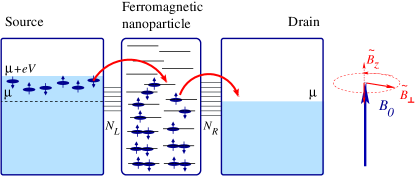
We assume that the single-electron spectrum of the particle, which is also called a quantum dot in the literature, to be chaotic and described by the random-matrix theory BeenakkerRMP ; ABG . To take into account the electron-electron interactions in the dot we use the universal Hamiltonian,Kurland2000 with a generalized spin part, corresponding to a ferromagnetic particle. Electrons occupy the quantum states of the full Hamiltonian and form a net spin of the particle of order of ; throughout the paper we use . The dot is coupled to two leads, see Fig. 1, which we assumed to be non-magnetic. The approach can be easily extended to the case of magnetic leads. The number of the transverse channels in the leads, which are well coupled to the dot, is assumed to be large, . Equivalently, the escape rate of electrons from the dot into the leads is large compared to the single-electron mean level spacing in the dot. This coupling to the leads is responsible for tunnelling processes of electrons between states in the leads and in the dot with random spin orientation. As a result of such tunnelling events, the net spin of the particle changes. We show that this exchange of electrons gives rise both to the Gilbert damping and the magnetization noise in the presented model, and under conditions specified below, the time evolution of the particle spin is described by the stochastic LLG equation.
We study in detail the conditions for applicability of the stochastic approach. We find that these limits are set by three independent criteria. First, the contact resistance should be low compared to the resistance quantum, which is equivalent to . If this condition is broken, the statistics of the noise cannot be considered gaussian. Physically, this condition means that each channel can be viewed as an independent source of noise, so the contribution of many channels results in the gaussian noise by virtue of the central limit theorem if . Second, the system should not be too close to the Stoner instability: the mean-field value of the total spin . If this condition is violated, the fluctuations of the absolute value of the magnetization become of the order of the magnetization itself. Third, , where is the effective temperature of the system, which is the energy scale of the electronic distribution function determined by a combination of temperature and bias voltage (the Boltzmann constant throughout the paper). Otherwise, the separation of the degrees of freedom into slow (the direction of the magnetization) and fast (the electron dynamics and the fluctuations of the absolute value of the magnetization) is not possible.
In the present model we completely neglect the spin-orbit interaction inside the particle, whose effect is assumed to be weak as compared to the effect of the leads.Tserkovnyak2002 The effects of the electron-electron interaction in the charge channel (weak Coulomb blockade) are suppressed for ,ABG so we do not consider it.
As an application of the formalism, we consider the magnetic susceptibility in the ferromagnetic resonance measurements, which is a standard characteristic of magnetic samples. Recently, a progress was reported in measurements of the magnetic susceptibility on small spatial scales in response to high-frequency magnetic fields.Tamaru2002 Measurements of the ferromagnetic resonance were also reported for nanoparticles, connected to leads for a somewhat different setup in Ref. Sankey2006, .
The paper is organized as follows. In Sec. II we introduce the model for electrons in a small metallic particle subject to Stoner instability. In Sec. III we analyze the effective bosonic action for the magnetization of the particle. In Sec. IV we obtain the equation of motion for the magnetization with the stochastic Langevin term, which has the form of the stochastic Landau-Lifshitz-Gilbert equation, and derive the associated Fokker-Planck equation. In Sec. V we discuss the conditions for the applicability of the approach. In Sec. VI we calculate the magnetic susceptibility from the stochastic LLG equation.
II Model and basic formalism
Within the random matrix theory framework, electrons in a closed chaotic quantum dot are described by the following fermionic action:
| (1) |
Here is a two-component Grassmann spinor, runs along the Keldysh contour, as marked by ; are the Pauli matrices (we use the hat to indicate matrices in the spin space and use the notation for the unit matrix). is an random matrix from a gaussian orthogonal ensemble, described by the pair correlators:
| (2) |
Here is the mean single-particle level spacing in the dot.
The magnetization energy is the generalization of the term in the universal Hamiltonian for the electron-electron interaction in a chaotic quantum dot.Kurland2000 Since we are going to describe a ferromagnetic state with a large value of the total spin on the dot, we must go beyond the quadratic term; in fact, all terms should be included. can be viewed as the sum of all irreducible many-particle vertices in the spin channel, obtained after integrating out degrees of freedom with high energies (above Thouless energy); the corresponding term in the action is thus local in time, and can be written as the time integral of an instantaneous function . This functional can be decoupled using the Hubbard-Stratonovich transformation with a real vector field , which we call below the internal magnetic field:
| (3) |
We rewrite the action in the form
| (4) |
where the inverse Green’s function
| (5) |
is a matrix in time variables , in orbital indices and with , in spin indices, and in forward () and backward () directions on the Keldysh contour. Integration over fermionic fields yields the purely bosonic action:
| (6) |
where the trace is taken over all indices of the Green’s function, listed above.
In the space of forward and backward directions on the Keldysh contour, we perform the standard Keldysh rotation, introducing the retarded (), advanced (), Keldysh (), and zero () components of the Green’s function:
| (7) |
as well as the classical () and quantum () components of the field:
| (8) |
We will also write this matrix as , where and are matrices in the Keldysh space coinciding with the unit matrix and the first Pauli matrix, , respectively.
The saddle point of the bosonic action Eq. (6) is found by the first order variation with respect to , which gives the self-consistency equation:
| (9) |
We also note that the right-hand side of this equation is proportional to the total spin of electrons of the particle for a given trajectory of :
| (10) |
In Eqs. (9) and (10), the trace is taken over orbital and spin indices only.
In the limit , one can obtain a closed equation for the Green’s function traced over the orbital indices:Ahmadian2005
| (11) |
The matrix satisfies the following constraint:
| (12) |
where the right-hand side is just the direct product of unit matrices in the spin, Keldysh, and time indices. The Wigner transform of is related to the spin-dependent distribution function of electrons in the dot:
| (13) |
In equilibrium, .
The self-consistency condition (9) takes the form
| (14) |
The last term takes care of the anomaly arising from non-commutativity of the limits and .
In this paper we consider the dot coupled to two leads, identified as left () and right (). The leads have and transverse channels, respectively, see Fig 1. For non-magnetic leads and spin-independent coupling between the leads and the particle, we can characterize each channel by its transmission with and by the distribution function of electrons in the channel , assumed to be stationary. We consider the limit of strong coupling between the leads and the particle, .
The coupling to the leads gives rise to a self-energy term, which should be included in the definition of the Green’s function, Eq. (5). Without going into details of the derivation, presented in Ref. Ahmadian2005, , we give the final form of the equation for the Green’s function traced over the orbital states, Eq. (11):
| (15) |
Here the products of functions include convolution in time variables. This equation is analogous to the Usadel equation used in the theory of dirty superconductors.Usadel1970
To conclude this section, we discuss the dependence . Deep in the ferromagnetic state, i.e. far from the Stoner critical point, we expect the mean-field approach to give a good approximation for the total spin of the dot. Namely, the mean field acting on the electron spins, is given by . We then require that the response of the system to this field gives the same average value for the spin:
| (16) |
Here we evaluated from Eq. (10) and applied the self-consistency equation (14) to equilibrium state with , when the contribution of the first term in the right hand side of Eq. (14) vanishes.
Not expecting strong deviations of the magnitude of the spin from the mean-field value, we focus on the form of when . The inverse Fourier transform of Eq. (3) and angular integration for the isotropic gives
| (17) |
where is the infinitesimal time increment used in the construction of the functional integral in Eq. (3).
Expanding near the mean-field value ,
| (18) |
performing the integration in the stationary phase approximation and using , we obtain
| (19) |
where is independent term. This expression for defines the action , Eq. (6).
The energy does not contain the energy , associated with the orbital motion of electrons in the particle. Namely, to form a total spin of the particle, we have to redistribute electrons over orbital states, which changes the orbital energy of electrons by . The total energy of the particle is the sum of two terms: . Similarly, we obtain the total energy of the system in terms of internal magnetic field
| (20) |
where does not depend on . We notice that the extremum of corresponds to and describes the expectation value of the internal magnetic field in an isolated particle. The energy cost of fluctuations of the magnitude of the internal magnetic field is characterized by the coefficient .
III Keldysh action
In this Section we analyze the action Eq. (6) for the internal magnetic field . We expect that the classical component of this field contains fast and small oscillations of its magnitude around the mean-field value . We further expect that the orientation of changes slowly in time, but is not restricted to small deviations from some specific direction. Based on this picture, we introduce a unit vector , assumed to depend slowly on time, and write
| (21) |
where is assumed to be fast and small. We expand the action (6) to the second order in small fluctuations of the quantum component and the radial classical component :
| (22) | |||||
The applicability of this quadratic expansion is discussed in Sec. V.2.
In Eq. (22) we introduced the polarization operator, defined as the kernel of the quadratic part of the action of the fluctuating bosonic fields:
| (23e) | |||
| (23f) | |||
where and . The short time anomaly is explicitly taken into account in the definition of the polarization operators, see Eq. (34) below.
The first term of Eq. (22) contains the vector of the Keldysh component of the Green function . We emphasize that the Green’s function and the polarization operator in Eq. (22) are calculated at and for a given trajectory of the classical field .
III.1 Keldysh component of the Green function
For the Green’s function in the classical field we have
| (24) |
while the Keldysh component satisfies the equation
| (25) |
We introduce the notation
| (26) |
Then the scalar and vector components of satisfy two coupled equations:
| (27a) | |||
| (27b) | |||
As a zero approximation, we can consider the stationary situation: and . In this case, we have
| (28) |
and .
For an arbitrary time dependence , Eq. (27b) cannot be solved analytically. However, if the variation of is slow enough, we can make a gradient expansion:
| (29) |
Here we introduced , , . The dependence on is split off and remains unchanged, while for the dependence on the solution is determined by a linear operator :
| (30a) | ||||
| (30b) | ||||
Here we assume that the direction of the internal magnetic field changes slowly in time, and .
Thus, all perturbations of decay with the characteristic time . In particular, the solution of Eq. (29) has the form
| (31) |
Expression for the first term in Eq. (22) can be easily obtained from Eq. (31) by taking the limit and taking into account that any fermionic distribution function in the time representation has the following equal-time asymptote:
| (32) |
We have
| (33) |
We notice that , and therefore the first term in the action Eq. (22) is coupled only to the tangential fluctuations of .
III.2 Polarization operator
We express the polarization operator in terms of the unit vector . The polarization operator can be represented as the response of the Green’s functions to a change in the field, as follows directly from the definition (23f) and the expression (6) for the action:
| (34) |
Here the Green function can be calculated as the first-order response of the solution of Eq. (LABEL:openUsadel=) to small arbitrary (in all three directions) increments of and . The zero-order solution of Eq. (LABEL:openUsadel=) in the field and is
| (35) |
First, we calculate , which responds only to :
| (36) |
Since , the solution always remains proportional to :
| (37) |
Given , components can be found either from Eq. (LABEL:openUsadel=), or, equivalently, using the constraint :
| (38) |
We notice that both respond only to and, therefore,
| (39) |
This equation ensures that the action along the Keldysh contour vanishes for .
To evaluate the remaining three components of the polarization operator, we can apply the variational derivatives to the sum of with respect to either classical or quantum field, which give and , respectively. Then, the advanced component .
To calculate the retarded component of the polarization operator, we calculate the response of to in the limit . Using the asymptotic behavior of the Fermi function, Eq. (32), we obtain:
| (41) |
Substituting this expression for to Eq. (34), we obtain
| (42a) | |||||
| with | |||||
| (42b) | |||||
Here we represented the polarization operator as a sum of the radial, , and tangential, , terms. We note that the action Eq. (22) contains only the radial component of the retarded and advanced polarization operators because we do not perform expansion in terms of the tangential fluctuations of the classical component of the field .
In response to , both corrections and contain terms , However, their sum remains finite in the limit :
| (43a) | ||||
| (43b) | ||||
with and .
From Eq. (43) we obtain the following expression for the Keldysh component of the polarization operator:
| (44a) | ||||
| (44b) | ||||
| (44c) | ||||
Here function coincides with the noise power of electric current through a metallic particle in the approximation of non-interacting electrons
| (45) |
In principle, electron-electron interaction in the charge channel can be taken into account. The interaction modifies the expression Eq. (45) for to the higher orderCV07 in and we neglect this correction here.
In this paper we consider a particle connected to electron leads at temperature with the applied bias . In this case, with , and the integration over gives
| (46) |
where
| (47) |
and is the ”Fano factor” for a dot
| (48) |
At the function has two scales of : (i) smears the non-analyticity at , but the value of deviates from at . Thus, the typical time scale above which one can approximate by a constant is at least . In the limit we have
| (49) |
The effective temperature is given by
| (50) |
III.3 Final form of the action
We can rewrite the action for magnetization field with in the form of Eq. (21) as a sum of the radial and tangential terms:
| (51) |
The radial term in the action has the form
| (52) |
where the inverse function of the internal magnetic field propagator is given by
| (53) |
and . From this equation we find
| (54) |
and . The Keldysh component is
| (55) |
The tangential term in the action is
| (56) |
Here we recovered the external magnetic field . The polarization operator is given by Eq. (44c).
IV Langevin equation
IV.1 Langevin equation for the direction of the internal magnetic field
In this section we consider evolution of the direction vector , described by the tangential terms in the action, Eq. (56). We neglect fluctuations of the magnitude of the internal magnetic field, , the conditions when these fluctuations can be neglected are listed in the next section.
We decouple the quadratic in component of the action in Eq. (56) by introducing an auxiliary field with the probability distribution
| (57) |
and the correlation function
| (58) |
The field plays the role of the gaussian random Langevin force. Integration of the tangential part of the action, Eq. (56), over produces a functional -function, whose argument determines the equation of motion:
| (59) |
The above equation can be resolved with respect to :
| (60) |
This equation is the Langevin equation for the direction of the internal magnetic field in the presence of the external magnetic field and the Langevin stochastic forces .
IV.2 The Fokker-Plank equation
Next, we follow the standard procedure of derivation of the Fokker-Plank equation for the distribution of the probability for the internal magnetic field to point in the direction . The probability distribution satisfies the continuity equation:
| (61) |
where the probability current is defined as
| (62) |
and the stochastic velocity is introduced in terms of the field as
| (63) |
The derivative is understood as the differentiation with respect to local Euclidean coordinates in the tangent space. Performing averaging over fluctuations of in Eq. (62), we obtain
| (64) |
where the time constant is defined as
| (65) |
Below we use the polar coordinates for the direction of the internal magnetic field, . In this case the Fokker-Plank equation can be rewritten in the form
| (66) |
where
| (67) | |||||
| (68) | |||||
It should be supplemented by the normalization condition:
| (69) |
which is preserved if the boundary conditions at are imposed:
| (70) |
Below we apply the Fokker Plank equation for calculations of the magnetization of a particle
| (71) |
V Applicability of the approach
In this section we discuss the conditions of validity of the stochastic LLG equation, see Eq. (66), for the model of ferromagnetic metallic particle connected to leads at finite bias. We briefly listed these conditions in the Introduction. Here we present their more detailed quantitative analysis.
V.1 Fluctuations of the radial component of the internal magnetic field
We represented the classical component of the internal magnetic field in terms of a slowly varying direction and fast oscillations of its magnitude around the average value . Now, we evaluate the amplitude of oscillations of the radial component of the field, using the radial term in the action, see Eqs. (51) and (52).
The typical frequencies for time evolution of small fluctuations of the internal magnetic field in the radial direction are of order of
| (72) |
as one can conclude from the explicit form of the propagator , Eq. (54), of these fluctuations. This scale has the meaning of the inverse -time in the spin channel. Deep in the ferromagnetic state (i. e., far from the Stoner critical point ) we estimate (which is equivalent to ), so this spin-channel -time is of the same order as the escape time . This estimate for the frequency range is consistent with the simple picture, which describes the evolution of the internal magnetic field of the grain as a response to a changing value of the total spin of the particle due to random processes of electron exchange between the dot and the leads. The electron exchange happens with the characteristic rate .
The correlation function can be evaluated by performing the Gaussian integration with the quadratic action in and . Using Eq. (55), we obtain the equal-time correlation function
| (73) |
This equation gives the value of fluctuations of the radial component of the internal magnetic field of the particle. These fluctuations survive even in the limit and , when . We have the following estimate
| (74) |
the upper cutoff is the Thouless energy, for a ballistic dot with diameter and electron Fermi velocity .
The separation of the internal magnetic field into the radial and tangential components is justified, provided that the fluctuations of the radial component are much smaller than the average value of the field , i.e. . Using the estimate Eq. (74), we obtain the necessary requirement for the applicability of equations for the slow evolution of the vector of the internal magnetic field of a particle:
| (75) |
where is the spin of a particle in equilibrium and we again used the estimate . Condition of Eq. (75) requires that the system is not close to the Stoner instability.
V.2 Applicability of the gaussian approximation
Let us discuss the applicability of the gaussian approximation for the action in and . The coefficients in front of terms are obtained by taking the th variational derivative of , or, equivalently, by iterating the Usadel equation times. Since the typical frequencies of are , the left-hand side of the equation is , while the right-hand side is . Since the only time scale here is , all the coefficients of the expansion of the action in at are of the same order:
| (76) |
At the same time, the typical value of , as determined by the gaussian part of the action, was estimated in the previous subsection to be of the order of , so the higher-order terms are indeed not important.
For the quantum component of the field the quadratic and quartic terms in the action are estimated as
| (77) |
If , then the typical frequency scale is , so the quadratic term gives , and . If , at the typical scale we obtain , so again for .
Physically, the parameter (or , if it is larger) can be identified with the number of the independent sources of the noise acting on the magnetization field. Thus, the smallness of the non-gaussian part of the action is nothing but the manifestation of the central limit theorem.
V.3 Applicability of the Fokker-Plank equation
From the above analysis we found that evolution of the direction of the internal magnetic field in time is described by a characteristic time , introduced in Eq. (65). From the analysis of the fluctuations of the magnitude of the internal magnetic field, see Eq. (72), we obtain the following condition when the separation into slow and fast variables is legitimate. The criterium can be formulated as , which can be presented as
| (78) |
VI Magnetic susceptibility of metallic particles out of equilibrium
The LLG equation derived in this paper for a ferromagnetic particle with finite bias between the leads can be applied to a number of experimental setups. Moreover, the derivation of the equation can be generalized to spin-anisotropic contacts with leads or Hamiltonian of electron states in the particle. In this paper we apply the stochastic equation for spin distribution function to the analysis of the magnetic susceptibility at finite frequency. The susceptibility is the basic characteristic of magnetic systems, it can often be measured directly, and determines other measurable quantities.
Below, we calculate the susceptibility of an ensemble of particles placed in constant magnetic field of an arbitrary strength and oscillating weak magnetic field, see Fig. 1. We consider the oscillating magnetic field with its components in directions parallel and perpendicular to the constant magnetic field.
VI.1 Solution at zero noise power
At when , and at fixed direction of the field, , equation of motion (60) is easily integrated for an arbitrary time dependence :
| (79) | |||||
| (80) |
Here the direction of magnetic field corresponds to .
VI.2 Constant magnetic field
At finite in constant magnetic field the Fokker-Plank equation has a simple solution
| (81) |
where the strength of constant magnetic field is written in terms of the dimensionless parameter
| (82) |
Substituting this probability function to Eq. (71), we obtain the classical Langevin expression for the magnetization of a particle in a magnetic field
| (83) |
This expression for the magnetization coincides with the magnetization of a metallic particle in thermal equilibrium, provided that the temperature is replaced by the effective temperature defined by Eq. (50).
The differential dc susceptibility is equal to
| (84) |
VI.3 Longitudinal susceptibility
We now consider the response of the magnetization to weak oscillations of the external magnetic field with frequency in direction parallel to the fixed magnetic field . We write the oscillatory component of the field in terms of the dimensionless field strength:
| (85) |
The linear correction to the probability distribution can be cast in the form
| (86) |
with defined by Eq. (81). The magnetic ac susceptibility can be evaluated from Eq. (86) as
| (87) |
The equation for is obtained from Eq. (66) with :
| (88) |
where we introduced the dimensionless frequency
| (89) |
and the time constant is defined in Eq. (65).
Note the symmetry of Eq. (88) with respect to the simultaneous change and . Also, the normalization condition for the probability function requires that
| (90) |
The latter holds if the boundary conditions Eq. (70) are satisfied, which in the case of axial symmetry can be written as
| (91) |
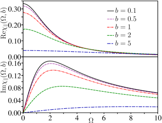
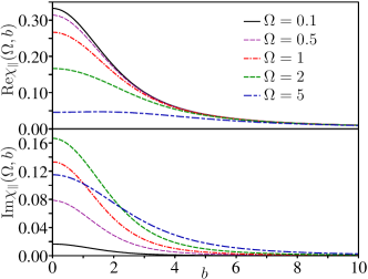
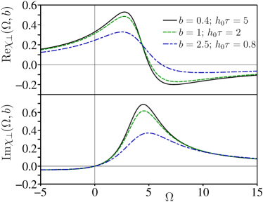
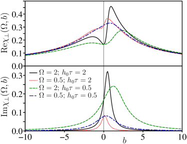
The differential equation (88) with the boundary condition Eq. (91) can be solved numerically and then the susceptibility is evaluated according to Eq. (87). The result is shown in Figs. 2 and 3, where the susceptibility is shown as a function of frequency or magnetic field , respectively. We also consider various asymptotes for the ac susceptibility, obtained from the solution of Eq. (88).
At zero constant magnetic field, , we find the exact solution of Eq. (88) explicitly:
| (92) |
This solution allows us to calculate the ac susceptibility in the form
| (93) |
For only matter, and we can find a specific solution of the inhomogeneous equation:
| (94) |
The requirement of regularity at the opposite end can be replaced by the probability normalization condition, Eq. (90), which is satisfied by this solution. Substituting this solution to Eq. (87), we obtain the strong field asymptote for the ac susceptibility
| (95) |
For and , we can neglect the derivatives in Eq. (88) and find the solution in the form
| (96) |
This solution also satisfies Eq. (90). For the susceptibility, Eq. (87), we obtain
| (97) |
Finally, the low frequency limit can be also analyzed analytically. The real part of the susceptibility coincides with the differential susceptibility in dc magnetic field, Eq. (84), for the imaginary part to the first order in frequency we obtain, see Appendix,
| (98) |
The function has a complicated analytical form and is not presented here, but its plot is shown in Fig. 4.
In all considered four limiting cases, the asymptotic approximations hold regardless the order in which the limits are taken. Indeed, the asymptote of the expression for the susceptibility in the zero field, Eq. (93), has the asymptote at consistent with Eq. (97) at . Similarly, the high frequency limit of Eq. (95) coincides with the limit of Eq. (97). Both limits of weak and strong magnetic field of the imaginary part of the susceptibility at low frequencies, Eq. (98), coincide with the imaginary part of , calculated from Eq. (93) and Eq. (97), respectively.
In general, we make a conjecture that the ac susceptibility is given by the following expression:
| (99) |
where functions and are real and describe the degeneracy points of the homogeneous differential equation Eq. (88) with real . This expansion is related to the expansion of time-dependent Fokker-Plank equations in the spherical harmonics, analyzed in Ref. Brown1963, . In particular, and .
For practical purposes, we found from a numerical analysis that even the single-pole approximation,
| (100) |
gives a very good estimate of the susceptibility for all values of and . The analysis shows that the susceptibility, Eq. (87), obtained from a numerical solution of Eq. (88), is within a few per cent of the estimate given by Eq. (100). The characteristic time constant, , as a function of magnetic field is chosen from the high frequency asymptote Eq. (97):
| (101) |
To evaluate the accuracy of the above approximation, Eq. (100), we consider the opposite limit of low frequencies, , and compare the exact result for the imaginary part of the susceptibility, Eq. (98), with
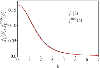
| (102) |
For visual comparison of functions and , we plot both functions in Fig. 4, where these curves are nearly indistinguishable. The difference between these two curves vanishes at and , and has a maximal difference at , which constitutes only tiny fraction of .
VI.4 Transverse susceptibility
Next, we consider the response of the magnetization to weak oscillations of the external magnetic field with frequency in direction perpendicular to the fixed magnetic field . We write the oscillatory component of the field in the form:
| (103) |
This field represents a circular polarization of an ac magnetic field in the plane, perpendicular to the fixed magnetic field in the -direction: . We look for the linear correction to the probability distribution in the form
| (104) |
The equation for is obtained from the Fokker-Plank equation Eq. (66), linearized in the parameter :
| (105) |
Here the dimensionless frequency is a difference between the drive frequency and the precession frequency in external field :
| (106) |
where is defined in Eq. (65) and the right equality is written in terms of dimensionless variables , Eq. (89), and , Eq. (82). Equation (105) is symmetric with respect to the simultaneous change , , , (“parity”). The function is single-valued at the poles and , only if
| (107) |
The latter equations establish the boundary conditions for the differential equation (105). We also note that the normalization condition is satisfied for any function .
We define the susceptibility in response to the ac magnetic field, Eq. (103), as
| (108) |
This expression for the susceptibility can be used to calculate the magnetization of a particle
| (109) |
to the lowest order in the ac magnetic field. In particular,
| (110) |
Solving numerically the differential equation (105) with the corresponding boundary conditions, Eq. (107), we obtain the transverse susceptibility, Eq. (108), shown in Figs. 5 and 6. Below we analyze several limiting cases.
In zero fixed magnetic field, , we have the exact solution of Eq. (105):
| (111) |
This solution corresponds to the solution in the longitudinal case, rotated by 90∘, cf. Eq. (92).
At and , the solution of Eq. (105) has a simple form and corresponds to a tilt of the external field. The susceptibility due to such tilt is
| (112) |
In strong fixed magnetic field, , we need to consider small angles , therefore, we can approximate in Eq. (105) and obtain:
| (113) |
The susceptibility in the limit is given by
| (114) |
t
At we can disregard the terms in Eq. (105) with derivatives. Moreover, the contribution to the susceptibility, Eq. (108), from the vicinity of and is suppressed as . This observation allows us to write the solution in the form
| (115) |
Consequently, we obtain the following high frequency, , asymptote for the susceptibility:
| (116) |
We can use the approximate expression for the susceptibility in response to the transverse oscillating magnetic field
The corresponding characteristic time constant can be found for any from the asymptotic behavior of at :
| (117) |
VII Conclusions
We have studied the slow dynamics of magnetization in a small metallic particle (quantum dot), where the ferromagnetism has arisen as a consequence of Stoner instability. The particle is connected to non-magnetic electron reservoirs. A finite bias is applied between the reservoirs, thus bringing the whole electron system away from equilibrium. The exchange of electrons between the reservoirs and the particle results in the Gilbert dampingGilbert55 of the magnetization dynamics and in a temperature- and bias-driven Brownian motion of the direction of the particle magnetization. Analysis of magnetization dynamics and transport properties of ferromagnetic nanoparticles is commonly performedPalacios1998 ; Usadel2006 ; Foros2007 ; Denisov2007 ; Kamenev2008 within the stochastic Landau-Lifshitz-Gilbert (LLG) equation LL35 ; Gilbert55 , which is an analogue of the Langevin equation written for a unit three-dimensional vector.
We derived the stochastic LLG equation from a microscopic starting point and established conditions under which the description of the magnetization of a ferromagnetic metallic particle by this equation is applicable. We concluded that the applicability of the LLG equation for a ferromagnetic particle is set by three independent criteria. (1) The contact resistance should be low compared to the resistance quantum, which is equivalent to . Otherwise the noise cannot be considered gaussian. Each channel can be viewed as an independent source of noise and only the contribution of many channels results in the gaussian noise by virtue of the central limit theorem for . (2) The system should not be too close to the Stoner instability: the mean-field value of the total spin . Otherwise, the fluctuations of the absolute value of the magnetization become of the order of the magnetization itself. (3) , where is the effective temperature of the system, which is the energy scale of the electronic distribution function. Otherwise, the separation into slow (the direction of the magnetization) and fast (the electron dynamics and the magnitude of the magnetization) degrees of freedom is not possible.
Under the above conditions, the dynamics of the magnetization is described in terms of the stochastic LLG equation with the power of Langevin forces determined by the effective temperature of the system. The effective temperature is the characteristic energy scale of the electronic distribution function in the particle determined by a combination of the temperature and the bias voltage. In fact, for a considered here system with non-magnetic contacts between non-magnetic reservoirs and a ferromagnetic particle the power of the Langevin forces is proportional to the low-frequency noise of total charge current through the particle. We further reduced the stochastic LLG equation to the Fokker-Planck equation for a unit vector, corresponding to the direction of the magnetization of the particle. The Fokker-Plank equation can be used to describe time evolution of the distribution of the direction of magnetization in the presence of time-dependent magnetic fields and voltage bias.
As an example of application of the Fokker-Plank equation for the magnetization, we have calculated the frequency-dependent magnetic susceptibility of the particle in a constant external magnetic field (i. e., linear response of the magnetization to a small periodic modulation of the field, relevant for ferromagnetic resonance measurements). We have not been able to obtain an explicit analytical expression for the susceptibility at arbitrary value of the applied external field and frequency; however, analysis of different limiting cases has lead us to a simple analytical expression which gives a good agreement with the numerical solution of the Fokker-Planck equation.
Acknowledgements
We acknowledge discussions with I. L. Aleiner, G. Catelani, A. Kamenev and E. Tosatti. M.G.V. is grateful to the International Centre for Theoretical Physics (Trieste, Italy) for hospitality.
Appendix A Longitudinal susceptibility at low frequencies
We find the linear in frequency correction to the dc susceptibility. For this purpose, we look for a solution to Eq. (88) in the form
| (118) |
where is the solution of Eq. (88) at and . We choose
| (119) |
since this form of preserves the normalization condition (90). This function can be found directly as a solution of Eq. (88) with or as a variational derivative of function , defined in Eq. (81), with respect to .
The linear in correction is the solution to the differential equation
| (120) |
From this equation, we can easily find
| (121) |
We notice that the solution to the latter equation will automatically satisfy the boundary conditions, given by Eq. (91). Integrating Eq. (121) once again, we obtain the following expression for function :
| (122) |
Here the integration constant has to be chosen to satisfy the normalization condition, Eq. (90), which results in complicated expression for the final form of the function .
References
- (1) W. F. Brown, Jr., Phys. Rev. 130, 1677 (1963).
- (2) L. Landau and E. Lifshitz, Phys. Z. Sowietunion 8, 153 (1935).
- (3) T. Gilbert, Phys. Rev. 100, 1243 (1955).
- (4) J. L. García-Palacios and F. J. Lázaro, Phys. Rev. B 58, 14937 (1998).
- (5) K. D. Usadel, Phys. Rev. B 73, 212405 (2006).
- (6) J. Foros, A. Brataas, G. E. W. Bauer, and Y. Tserkovnyak, Phys. Rev. B 75, 092405 (2007).
- (7) S. I. Denisov, K. Sakmann, P. Talkner, and Hänggi, Phys. Rev. B 75, 184432 (2007).
- (8) A. Rebei and M. Simoniato, Phys. Rev. B 71, 174415 (2005).
- (9) H. Katsura, A. V. Balatsky, Z. Nussinov, and N. Nagaosa, Phys. Rev. B 73, 212501 (2006).
- (10) A. S. Núñez and R. A. Duine, Phys. Rev. B 77, 054401 (2008).
- (11) A. L. Chudnovskiy, S. Swiebodzinski, and A. Kamenev, Phys. Rev. Lett. 101, 066601 (2008).
- (12) J. Foros, A. Brataas, Y. Tserkovnyak, and G. E. W. Bauer, Phys. Rev. Lett. 95, 016601 (2005).
- (13) R. A. Duine, A. S. Núñez, J. Sinova, and A. H. MacDonald, Phys. Rev. B 75, 214420 (2007).
- (14) X. Waintal and P. W. Brouwer, Phys. Rev. Lett. 91, 247201 (2003).
- (15) I. L. Aleiner, P. W. Brouwer, and L. I. Glazman, Phys. Reports 358, 309 (2002).
- (16) C. W. J. Beenakker, Rev. Mod. Phys. 69, 731 (1997).
- (17) I. L. Kurland, I. L. Aleiner, and B. L. Altshuler, Phys. Rev. B 62, 14886 (2000).
- (18) Y. Tserkovnyak, A. Brataas, and G. E. W. Bauer, Phys. Rev. Lett. 88, 117601 (2002).
- (19) S. Tamaru et al., J. Appl. Phys. 91, 8034 (2002).
- (20) J. C. Sankey et al., Phys. Rev. Lett. 96, 227601 (2006).
- (21) Y. Ahmadian, G. Catelani, and I. L. Aleiner, Phys. Rev. B 72, 245315 (2005).
- (22) K. D. Usadel, Phys. Rev. Lett. 25, 507 (1970).
- (23) G. Catelani and M. G. Vavilov, Phys. Rev. B 76, 201303 (2007).