Physical time and other conceptual issues of QG on the example of LQC

Abstract

Abstract:  Several conceptual aspects of quantum gravity are studied on the example of the homogeneous isotropic LQC model. In particular: $(i)$ The proper time of the co-moving observers is showed to be a quantum operator and a quantum spacetime metric tensor operator is derived. $(ii)$ Solutions of the quantum scalar constraint for two different choices of the lapse function are compared and contrasted. In particular it is shown that in case of model with masless scalar field and cosmological constant $\Lambda$ the physical Hilbert spaces constructed for two choices of lapse are the same for $\Lambda<0$ while they are significantly different for $\Lambda>0$. $(iii)$ The mechanism of the singularity avoidance is analyzed via detailed studies of an energy density operator, whose essential spectrum was shown to be an interval $[0,\rho_{{\rm cr}}]$, where $\rho_{{\rm cr}}\approx 0.41\rho_{\operatorname*{Pl}}$. $(iv)$ The relation between the kinematical and the physical quantum geometry is discussed on the level of relation between observables.

I Introduction: the issues raised in the paper

Loop Quantum Cosmology lqc1 ; lqc2 is a family of symmetry reduced models built via methods of Loop Quantum Gravity lqg . It serves both as a testing ground for the quantization frameworks used in Quantum Gravity lqc2 ; bahr ; kls-obs and also a shortcut way to derive some physical predictions. One of the most surprising predictions it provides is the modification of the dynamics at near-Planck energy densities leading to the replacement of the classical Big Bang by a quantum Big Bounce. Although the most solid and robust results were obtained for isotropic cosmological models aps ; aps-imp ; apsv-spher ; skl-spher ; frw-hyper ; sLQC ; kl-sadj ; eff , there is an ongoing research (with various stages of rigour) treating homogeneous but anisotropic B1 or even inhomogeneous models eff-als ; spher ; gm-letter . In this paper we are concerned with some conceptual aspects of quantum gravity and study them on the example of the homogeneous isotropic LQC model. They are: existence of a quantum spacetime metric tensor operator, definition of a solution to the quantum Einstein constraints, mechanism of singularity avoidance and the role of the kinematical quantum geometry for the properties of the physical quantum geometry.

Before going to the technical details of the LQC model used in this work, we will present an outline of our studies (in Sec. I.1 through I.5). Next, in Sec. II we will introduce the necessary technical details of the LQC model tested in this work, which is the model of isotropic, homogeneous spacetime interacting with a homogeneous scalar field introduced by Ashtekar, Pawlowski and Singh aps-imp . Most of our results apply also (either directly or can be generalized) to the so called solvable LQC (sLQC) model sLQC .

I.1 A quantum relativistic time, a quantum spacetime

One of the expectations upon the theory of quantum geometry is that it should provide a spacetime metric as a quantum operator

$$\widehat{{\rm d}s^{2}}\ =\ \widehat{g_{\alpha\beta}}{\rm d}x^{\alpha}{\rm d}x^{\beta}\ .$$ (1)

In the canonical formulation of the Einstein gravity, a general classical spacetime metric is written in the form

$${\rm d}s^{2}\ =\ -(N^{2}-N^{a}N^{b}q_{ab}){\rm d}t^{2}+N^{b}q_{ab}({\rm d}t{\rm d}x^{a}+{\rm d}x^{a}{\rm d}t)+q_{ab}{\rm d}x^{a}{\rm d}x^{b}\ .$$ (2)

In the gauge choice free approach, the lapse and shift functions $N$ and $N^{a}$ respectively, are just non-dynamical gauge parameters. Therefore they should pass unchanged to the quantum theory, allowing in turn to write the metric tensor in the form

$$\widehat{{\rm d}s^{2}}\ =\ -(N^{2}-N^{a}N^{b}\hat{q}_{ab}){\rm d}t^{2}+N^{b}\hat{q}_{ab}(t,x)({\rm d}t{\rm d}x^{a}+{\rm d}x^{a}{\rm d}t)+\hat{q}_{ab}(t,x){\rm d}x^{a}{\rm d}x^{b}\ ,$$ (3)

where the un-hatted functions are independent of $\hat{q}$. As a consequence, even in the quantum theory, the $g_{tt}$ metric component commutes with all the other quantum metric components at any given instant $t$.

However, since Einstein’s gravity is a theory with constraints, the physical Hilbert space differs from the kinematical one, and only the Dirac observables can give rise to physical quantum observables. Therefore, the spacetime metric should be first reexpressed in terms of them. A quite well understood class of the Dirac observables are the partial observables developed recently by Rovelli, Dittrich and Thiemann rel-obs . A partial observable is constructed out of a kinematical observable and a family of clock functions – functions defined on the classical phase space providing parametrizations of dynamical trajectories. One of possible choices of such clock function $T$ is a (coupled to the gravitational field) Klein-Gordon massless scalar field (which is exactly the choice made in the APS model of the quantum FRW spacetime aps-imp ). Upon that choice one can write the metric tensor (2) as,

$${\rm d}s^{2}\ =\ g_{TT}{\rm d}T^{2}+N^{\prime b}q^{\prime}_{ab}({\rm d}T{\rm d}x^{a}+{\rm d}x^{a}{\rm d}T)+q^{\prime}_{ab}{\rm d}x^{a}{\rm d}x^{b}\ .$$ (4)

The function $g_{TT}$ is of the form

$$g_{TT}\ =\ -\left(\frac{N^{2}-N^{a}N^{b}q_{ab}}{N\frac{\pi_{T}}{\sqrt{{\rm det}q}}+N^{a}T_{a}}\right)$$ (5)

where $\tilde{\pi}_{T}$ is the momentum canonically conjugate to $T$, and the second equality follows from the canonical equations

$$\frac{\partial T}{\partial t}\ =\ \{\,T,\,\int\frac{N}{2}(\frac{\tilde{\pi}_{T}^{2}}{\sqrt{\det q}}+q^{ab}\sqrt{{\rm det}q}T_{,a}T_{,b})\ +\ \int N^{a}\tilde{\pi}_{T}T_{,a}\}\ .$$ (6)

From (5) it follows immediately that, since all terms on its righthand side are dynamical quantities, so is the function $g_{TT}$. Thus in quantum theory one should consider a Dirac observable corresponding to it. Whereas on the kinematical Hilbert space the operators $\hat{\pi}_{T}$ and $\hat{q}_{ab}$ commute, the corresponding partial observables do not, therefore the quantum counterpart of the righthand side of (5) is not uniquely defined. This problem can be seen at the classical level already. Namely, if we denote by ${\cal O}_{\tilde{\pi}_{T}}$ and ${\cal O}_{q_{ab}}$ the corresponding Dirac observables (we suppress the clock functions and other parameters needed to determine the observable), then their Poisson bracket does not vanish. Indeed, (see GiesThiem-algiv for details)

$$\{{\cal O}_{\tilde{\pi}_{T}},\,{\cal O}_{q_{ab}}\}\ =\ {\cal O}_{\{{\tilde{\pi}_{T},q_{ab}}\}^{\rm D}}$$ (7)

where ${\cal O}_{F(f)}=F({\cal O}_{f})$ and $\{\cdot,\cdot\}^{D}$ is the Dirac bracket. Furthermore, one can show by inspection (using eq. (2.18) of GiesThiem-algiv ), that

$$\{{\tilde{\pi}_{T},q_{ab}}\}^{\rm D}\ \not=\ 0\ .$$ (8)

In consequence:

1. a quantum counterpart of $g_{TT}$ is an operator which does not commute with $\hat{q}_{ab}$ even at the same instant of time,

2. there is no unique definition of $\hat{g}_{TT}$ because of the ordering problem.

In this paper, we point out the issue and propose a definition of the quantum space-time metric tensor in the APS quantum FRW model, where the expression for the lapse function (5) reduces (due to homogeneity) to

$$g_{TT}\ =\ \frac{\sqrt{\det q}}{\tilde{\pi}_{T}}\ .$$ (9)

I.2 The physical meaning of the quantum geometry operators

The quantum geometry operators are defined in the kinematical Hilbert space. They are build, briefly speaking, out of the 3-metric tensor. The question regards the role and the properties of the quantum geometry operators in the physical Hilbert space. Considered operators can be defined by using the relational observables of Rovelli-Dittrich-Thiemann. On the one hand, they form in this case the same Poisson algebra as the kinematical ones. Also in simple examples ($\Lambda=0$) their quantum algebra is equivalent to the algebra of the kinematical quantum geometry operators. On the other hand, in the case of $\Lambda>0$ there are many differences between the kinematical and physical quantum geometry. We discuss them is Sec. III.

I.3 Dependence of solutions to the constraint on lapse

In a canonical approach to quantum gravity one has to define subsequently

• a quantum scalar constraint operator

• the constraint condition, that is the mechanism via which the constraint operator selects the physical Hilbert space

• a physical Hilbert space of solutions, which involves in particular specification of the scalar product on it.

In our case the quantum constraint operator has the form

$${\hat{C}_{{\rm tot}}}(N)\ =\ N(\frac{1}{2}{\hat{\pi}_{T}^{2}}\widehat{\sqrt{\det q}^{\ -1}}\ +\ {\widehat{C_{{\rm gr}}}})\ ,$$ (10)

where $N$ is the lapse. One choice is to take lapse to be a number.

On the other hand, taking into account (9) and the quantum nature of the lapse one is lead to the constraint operator

$${\hat{C}_{{\rm tot}}}(N^{\prime})\ =\ \frac{1}{2}{\hat{\pi}_{T}}\ +\ \hat{\pi}_{T}^{-1}\left[\widehat{{\sqrt{\det q}\,}^{-1}}\right]^{-1}{\widehat{C_{{\rm gr}}}}\ ,$$ (11)

suitably symmetrised in the second term

Given either one of the constraints, one can turn to the second step and define the corresponding constraint condition. It reads: take the spectral decomposition defined by the operator and allow only elements of the Hilbert space corresponding to the zero eigenvalue.

At this point we make a suprising discovery:

• On the one hand, the first operator (10) has a unique self-adjoint extension for arbitrary cosmological constant; we point it out in Section V and give a mathematical argument.

• On the other hand, the second operator (11) has inequivalent self-adjoint extensions if $\Lambda>0$.

In other words, the second constraint operator does not define a constraint condition uniquely, because the spectral decomposition depends of a self-adjoint extension. Hence, solutions to that quantum scalar constraint depend on some additional choice which has to be made. This apparent discrepancy forces us to ask a question: What is a relation between the uniquely defined Hilbert space of solutions of the constraint (10) and the extension dependent Hilbert spaces of solutions to the second constraint (11)?

To address it we explain in detail the difference in the properties of the operators (10) and, respectively, (11) in Sec. V. Also, we briefly discuss the relation between Hilbert spaces of the solutions to those different constraints (the detailed analysis will be presented in ga ).

I.4 Big-Bounce and the energy density operator

Within cosmological model specified at the end of Section I.1 the equality satisfied by the lapse function (now given by (9)) can be also written in the following way

$$N^{\prime 2}{\rm d}T^{2}\ =\ 2\rho^{-1}{\rm d}T^{2}$$ (12)

where

$$\rho\ =\ \frac{1}{2}\frac{\tilde{\pi}_{T}^{2}}{\det q}\ =\ T_{\mu\nu}n^{\mu}n^{\nu}$$ (13)

is the energy density of the scalar field with respect to the class of observers comoving with the universe.

The quantum energy density operator and its spectrum is another subject discussed in this paper on its own. The operator is used in the APS model as the measure of the avoidance of the singularity. At the early stages of LQC it was believed that the singularity avoidance is a kinematical effect implied by the non-singular way the metric determinant inverse shows up in the expression of the energy density. Indeed, the LQG motivated quantization of that expression has (up to factor ordering ambiguity) the form

$$\hat{\rho}\ =\ \frac{1}{2}\hat{\pi}_{T}^{2}\widehat{\det q^{-1}}\ ,$$ (14)

where the operator $\widehat{\det q^{-1}}$ is bounded, and actually annihilates the vector annihilated by $\widehat{\det q}$. A stronger result takes place in the APS model. Namely, the expectation value of the energy density $\langle\hat{\rho}\rangle(T)$ evolving with the time $T$ approaches certain universal value (of the order of Planck energy density $\rho_{\operatorname*{Pl}}$)

$$\langle\hat{\rho}\rangle(T)\ \leq\ \rho_{{\rm cr}}\ \approx\ 0.82\rho_{\operatorname*{Pl}}$$ (15)

from below, and bounces back. Here we show, that the essential spectrum of $\hat{\rho}$ is

$${\operatorname*{Sp}{}_{\operatorname*{es}}}(\hat{\rho})\ =\ [0,\rho_{{\rm cr}}]\ .$$ (16)

There may still exist discrete spectrum elements bigger then $\rho_{{\rm cr}}$, however, the corresponding eigenfunctions are focused near the zero volume and therefore their contribution to semiclassical states focused at large scalar field momentum (and so at large volumes) is extremely small.

I.5 The role of the zero volume state

A technical subtlety concerning the constraint operators above, is that in the APS model the zero volume state $|0\rangle\in{\cal H}_{\rm gr}$ is at the same time annihilated by the inverse-volume operator

$$\widehat{\sqrt{\det q}^{-1}}|0\rangle\ =\ 0\ .$$ (17)

This leads to an impression of incompleteness in a definition of the operator ${\hat{C}_{{\rm tot}}}(N^{\prime})$ in $({\mathcal{H}_{{\rm gr}}},\,(\cdot|\widehat{\sqrt{\det q}^{-1}}\cdot))$ present even after the modification of the scalar product which removes that zero volume state. The solution to that subtlety is hidden in the results published in the literature aps-imp ; apsv-spher ; negL , but it has never been spelled out. We will present the details in Sec. A showing in particular some constraint being induced in ${\mathcal{H}_{{\rm gr}}}$ by the scalar constraint operator. The presence of this constraint allowed to define rigorously the evolution operator in aps-imp and following works. The discussed structure allows in particular to immediately extend the results of kl-sadj to superselection sector containing the $|v=0\rangle$ state.

II The elements of the LQC FRW

In LQC, like in the other cosmological models, one restricts the Einstein’s theory to the space of the space-time metrics and other fields having a given symmetry. Here we consider the case of Friedman-Robertson-Walker (FRW) models corresponding to homogeneous and isotropic spacetimes. In this section we briefly introduce the quantum description of these models within LQC framework. For shortness we will introduce only those elements of the LQC models which will be relevant for our studies. For more detailed description of the quantization procedure the reader is referred to abl and aps-imp .

On the classical level the spacetime is described by the product manifold $\mathbb{R}\times\Sigma$ and a metric tensor

$${\rm d}s^{2}\ =\ -N^{2}{\rm d}t^{2}\ +\ a^{2}\,{}^{o}\!q_{ab}{\rm d}x^{a}{\rm d}x^{b}$$ (18)

where $\,{}^{o}\!q$ is a fixed, auxiliary, homogeneous, isotropic metric tensor on $\Sigma$, and $N$ is a homogeneous lapse function. The metric is coupled with a scalar field $T$ homogeneous on $\Sigma$. These properties boil down to conditions

$$a(t,x)\ =\ a(t)\ , T(t,x)\ =\ T(t)\ , N(t,x)\ =\ N(t)\ .$$ (19)

The diffeomorphism constraints are trivially satisfied, hence the only Einstein constraint is the scalar constraint. It takes the following form

$${\hat{C}_{{\rm tot}}}(N)\ =\ N({\widehat{C_{{\rm gr}}}}+\frac{1}{2}\frac{\tilde{\pi}_{T}^{2}}{|V|})\ ,$$ (20)

where one fixes a finite region (“cell”) ${\Sigma}_{0}\subset\Sigma$ to integrate (if $\Sigma$ is compact a natural choice is $\Sigma_{0}=\Sigma$)

$${\pi_{T}}\ :=\ \int_{\Sigma_{0}}{\tilde{\pi}}_{T}\ , |V|\ :=\ \int_{\Sigma_{0}}a^{3}\sqrt{{\rm det}q^{(0)}}\ , C_{\rm gr}\ =\ \int_{\Sigma_{0}}\tilde{C}_{\rm gr}$$ (21)

and $\tilde{C}_{\rm gr}$ is the Hamiltonian density of the gravitational field. One also introduces the oriented volume function ranging from $-\infty$ to $\infty$, namely

$$V\ =\ \pm|V|\ ,$$ (22)

with the sign depending on the orientation in $\Sigma_{0}$ of the triad with respect to a fixed fiducial orientation of $\Sigma$. The kinematical Hilbert space and the quantum operators of the scalar field $T$ and its conjugate momentum ${\pi_{T}}$ are

$${\cal H}_{\rm sc}\ =\ L^{2}({\mathbb{R}})\ ,$$ (23a)

$$\hat{T}\psi(T)\ =\ T\psi(T)\ ,\qquad {}\qquad\hat{\pi}_{T}\psi(T)\ =\ -i\hbar\partial_{T}\psi(T)\ .$$ (23b)

The kinematical Hilbert space and the basic quantum operators for the gravitational field in the APS and sLQC model are,

$${\mathcal{H}_{{\rm gr}}}\ =\ \overline{{\rm Span}(|v\rangle\ :\ v\in{\mathbb{R}})}\ , \langle v|v^{\prime}\rangle\ =\ \delta_{v,v^{\prime}}\ ,$$ (24a)

$$\hat{V}|v\rangle\ =\ \left(\frac{8\pi\gamma}{6}\right)^{\frac{3}{2}}\frac{3\sqrt{3\sqrt{3}}}{2\sqrt{2}}\,v\,\ell_{\operatorname*{Pl}}^{3}|v\rangle\ =:\ V_{o}\,v|v\rangle\ , \hat{h}_{\nu}|v\rangle\ =\ |v+\nu\rangle\ ,$$ (24b)

where the operator $\hat{h}_{\nu}$ is a shift operator – a component of an operator corresponding to the classical holonomy function involving $da/dt$.

The kinematical Hilbert space of the system is the tensor product ${\mathcal{H}_{{\rm sc}}}\otimes{\mathcal{H}_{{\rm gr}}}$. Every element $\psi\in{\mathcal{H}_{{\rm sc}}}\otimes{\mathcal{H}_{{\rm gr}}}$ is thought of as a function of the variables $T$ and $v$, and its values will be denoted by $\psi(T,v)$.

The quantum scalar constraint is considered in the following form

$$\left(\frac{1}{2}\hat{\pi}_{T}^{2}\otimes 1\ +\ 1\otimes\widehat{|V|^{-1}}^{-1}\widehat{C_{\rm gr}}\right)\,\psi(T,v)\ =\ 0\ ,$$ (25)

where:

• $\widehat{|V|^{-1}}=V_{o}^{-1}B(\hat{V})$ is a result of a quantization of the classical $1/|V|$, with $B$ being a function. In the orthodox LQC it descends from the LQG definition of the orthonormal coframe expressed by commutators of various powers of the volume operator. For the studies performed in this article the exact form of $B$ does not matter. What is important are the following properties (true for both APS LQC and sLQC)

  1. $B(v)=B(-v)$,

  2. for non zero $v$ is finite and nonvanishing, and

  3. for large $|v|$, $B(v)\simeq\frac{1}{|v|}$.

  More specific assumptions will be made whenever necessary. Particular form of $B$ in models considered here is, respectively,

  $$B_{\rm sLQC}(v)\ =\ \frac{1}{|v|}\ , B_{\rm APS}(v)\ =\ \frac{27}{8}|v|\big{|}|v+1|^{\frac{1}{3}}-{|v-1|}^{\frac{1}{3}}\big{|}^{3}\ .$$ (26)

• the operator $\widehat{C_{\rm gr}}$ has the form

  $$\widehat{C_{\rm gr}}\ =\ i(\hat{h}_{2}-\hat{h}_{-2})A(\hat{V})i(\hat{h}_{2}-\hat{h}_{-2})-\Lambda\hat{V}+W_{k}(\hat{V})$$ (27)

  with $\Lambda$ being the cosmological constant, and $A$, $W_{k}$ being suitable symmetric functions, the second one depending on the type of the local symmetry group ($k=-1,0,1$). The assumption about $A$ we will refer to is the behavior $A(v)\sim|v|$ for large $|v|$ true in LQC as well as in the sLQC. In these two particular cases the form of $A$ reads

  $$A_{\rm APS}\ =\ A_{o}\tilde{A}\ =\ A_{0}|v|\big{|}|v+1|-|v-1|\big{|}\ ,$$ (28a)

  $$A_{\rm sLQC}\ =\ 2A_{o}|v|\ , A_{o}\ :=\ \frac{9\sqrt{3}\ell_{\operatorname*{Pl}}}{32\sqrt{\pi}\gamma^{\frac{3}{2}}G}\ .$$ (28b)

The physical states are solutions to the quantum constraint, according to the APS model, thought of as maps

$$\mathbb{R}\ni T\ \mapsto\ \psi_{T}\in{\mathcal{H}_{{\rm gr},B}}\ ,$$ (29)

where the space ${\cal H}_{\rm gr,B}$ (referred to further as an auxiliary space) is defined by the same ${\rm Span}(|v\rangle\!:\ v\in{\mathbb{R}})$ as before, however endowed by APS with the scalar product

$$(\cdot|\cdot)_{B}\ =\ \langle\cdot|B(\hat{V})\cdot\rangle\ .$$ (30)

That definition of the new scalar product is suited to make the evolution operator

$$\hat{\Theta}\ :=\ -(B(\hat{V}))^{-1}{\widehat{C_{{\rm gr}}}}$$ (31)

symmetric, however the definition of this operator in the form it is presented above, needs to be completed. Such precise definition, which was used in aps-imp ; apsv-spher ; negL , is discussed in Appendix A. Now, each solution to the scalar constraint takes the form

$$\psi\ =\ \psi^{-}\ +\ \psi^{+}\ ,$$ (32)

where $\psi^{\pm}$ satisfies, respectively,

$$\hat{\pi}_{T}\psi^{\pm}_{T}(v)\ =\ \pm\sqrt{2V_{o}\hat{\Theta}}\,\psi^{\pm}_{T}(v)\ ,$$ (33)

where each solution $\psi$ of (33) takes values $\psi_{T}$ in the part of the Hilbert space corresponding to the non-negative part of the spectrum of the operator $\hat{\Theta}$, and the square root is defined on that subspace. We will be assuming throughout this paper that this decomposition is unique, which is generically true. A non-unique case is considered in posL1 . Given two solutions $\psi$ and $\psi^{\prime}$ of the quantum scalar constraint, APS define the following scalar product

$$(\psi|\psi^{\prime})_{\rm phys}\ :=\ (\psi^{+}_{T}|\psi^{+}_{T})_{B}\ +\ (\psi^{-}_{T}|\psi^{-}_{T})_{B}$$ (34)

where the RHS is independent of $T$. Denote the resulting Hilbert space by ${\mathcal{H}_{{\rm phys}}}$.

A physical observable $\hat{\pi}_{T}$ is

$$\hat{\pi}_{T}\psi^{\pm}\ :=\ \pm\sqrt{2V_{o}\hat{\Theta}}\,\psi^{\pm}\ ,$$ (35)

The volume operator $\hat{V}$ defined in the kinematical Hilbert space gives rise to the physical observable ${\hat{\cal O}}_{V}(T_{0})$ (modulo the discussion in Sec. III below) determined by a number $T_{0}$ (the “instant of time”) and defined by the following expression

$$({\hat{\cal O}}_{V}(T_{0})\psi)_{T_{0}}\ =\ \hat{V}\psi_{T_{0}}\ .$$ (36)

In consequence it can be thought of as an operator in QM acting at an instant $T_{0}$ on a state evolving in the Schroedinger picture.

The final Hilbert space is selected as the irreducible subspace of all the quantum observables we choose. Classically, the system can be described completely by scalar field momentum ${\pi_{T}}$ and the volume of the fixed cell $V$. The first one commutes with the constraint, whereas the second defines the Dirac observables via the relational observables construction. Therefore, APS assume that the sufficient set of quantum operators to describe every quantum state consists of the following operators:

$$\hat{\pi}_{T}\psi^{\pm}(T,v)\ :=\ (\mathbb{I}\times\sqrt{2V_{o}\hat{\Theta}})\,\psi^{\pm}(T,v)\ ,$$ (37a)

$$|\hat{V}|_{T_{0}}\psi^{\pm}(T,v)\ :=\ e^{\pm i(T-T_{0})\sqrt{2V_{o}\hat{\Theta}}}\,\hat{V}\,\psi^{\pm}(T_{0},v)\ .$$ (37b)

Furthermore, there are subspaces $\mathcal{H}^{\pm}_{{{\rm phys}},\epsilon}$ preserved by the action of all the quantum observables, labeled by arbitrary $\epsilon\in[0,4)$ and a sign ‘$+$’ or ‘$-$’ corresponding to the decomposition (32). The subspace ${\cal H}^{+}_{{\rm phys},\epsilon}$ (${\cal H}^{-}_{{\rm phys},\epsilon}$) is the space of solutions (29) to (33) with $\pm=+$ ($\pm=-$) which take values in the following subspace of ${\cal H}_{{\rm gr},B}$

$${\cal H}_{\epsilon}\ =\ \overline{{\rm Span}(|v\rangle\ :\ v=\epsilon+4n,\ \ n\in{\mathbb{Z}})}$$ (38)

In the special cases of $\epsilon=0,\,2$, the subspace ${\cal H}^{\pm}_{\epsilon}$ admits the action of the orientation changing operator

$$(P\psi)_{T}(v)\ \mapsto\ \psi_{T}(-v)\ .$$ (39)

which commutes with $T$. In that case APS restrict the Hilbert space ${\cal H}^{\pm}_{\epsilon}$ further, to the subspace of the even functions.

The operator $\hat{\Theta}$ is well defined in every subspace $\mathcal{H}^{\pm}_{\epsilon}$ (in the domain ${{\rm Span}(|v\rangle\ :\ v=\epsilon+4n,\ \ n\in{\mathbb{Z}})}$) such that $\epsilon\not=0$, however for $\epsilon=0$ its definition is not a priori obvious and needs explanation. We provide it in Appendix A as well as our definition of the evolution operator $\hat{\Theta}$ in the $B(0)=0$ case.

Remarks.

• For the remaining values of the parameter $\epsilon$ we have $P(\mathcal{H}^{\pm}_{\epsilon})=\mathcal{H}^{\pm}_{4-\epsilon}$. Then, APS construct the space of the even functions spanned by elements of $\mathcal{H}^{\pm}_{\epsilon}$ and $P(\mathcal{H}^{\pm}_{\epsilon})$. In these cases construction reduces (is unitarily equivalent) to the single $\mathcal{H}^{\pm}_{\epsilon}$.

• We will often ignore the reducibility and consider the whole Hilbert space $\mathcal{H}_{{\rm phys}}$.

III The quantum geometry operators in the physical theory

In the Dirac program one of the most common techniques of constructing observables on ${\mathcal{H}_{{\rm phys}}}$ is an appropriate pull-back onto it of kinematical ones. However unless the quantity measured by given observable is a constant of motion such direct pull-back will not correspond to any physically interesting property of the system. Therefore in such cases one tries to construct operators measuring kinematical quantity “at a given time” (example of which is the operator $|\hat{v}|_{\phi}$ defined in aps-imp ). Technically this corresponds to the pull-back of kinematical observable to an auxiliary Hilbert space, the image of mapping (29). In this section we address (in context of LQC) the question of how the original properties of kinematical operators transfer to physical spaces. We will see that even the volume operator, seemingly under a perfect control, may surprisingly change much more, than it is expected in the LQC literature.

Let us start our analysis in the context of an APS LQC, where $B(0)=0$. There the auxiliary Hilbert space is a space $\mathcal{H}_{{\rm gr},B}$ equipped with the modified scalar product $\langle\cdot|B(\hat{V})\cdot\rangle$. The quantum volume operator is unchanged by this modification, and is still well defined and essentially self-adjoint in the domain ${\rm Span}(|v\rangle\ :\ v\in\mathbb{R})$. However a general operator $\hat{g}$ defined in that domain in ${\cal H}_{\rm gr}$ should be redefined such that modulo the ordering it corresponds to the same classical kinematical observable, but has the correct properties with respect to the ^† operation. An example of such redefinition is replacing $\hat{g}$ defined in ${\cal H}_{\rm gr}$ by

$$B(\hat{V})^{-1/2}\hat{g}B(\hat{V})^{1/2}$$

defined in ${\cal H}_{{\rm gr},B}$. In fact, this transformation coincides with the pull back of $\hat{g}$ by the unitary map used in the previous section, which is

$$\mathcal{H}_{{\rm gr},B}\ \rightarrow\ {\mathcal{H}_{{\rm gr}}}\ , \psi\ \mapsto\ \sqrt{B(\hat{V})}\psi\ ,$$ (40)

and the inverse image of the domain ${\rm Span}(|v\rangle\ :\ v\in\mathbb{R})$ is ${\rm Span}(|v\rangle\ :\ 0\not=v\in\mathbb{R})$. As we mentioned, the volume operator $\hat{V}$ is not affected by that transformation (modulo the small restriction of the domain consisting in disappearing of the zero volume eigenvector $|0\rangle$.)

In the sLQC case, on the other hand, the auxiliary space is directly ${\mathcal{H}_{{\rm gr}}}$, so the analog of the transformation (40) is just an identity.

The transformation presented above does not however solve all the problems. To see that let us go back to the construction of the physical Hilbert space. To shorten the explanation we introduce the common notation denoting by $({\cal H},(\cdot|\cdot))$ the Hilbert space $({\cal H}_{{\rm gr},B},\langle\cdot|B\cdot\rangle)$ in the APS model case, or $({\cal H}_{{\rm gr}},\langle\cdot|\cdot\rangle)$ in the sLQC case. Then each element of ${\mathcal{H}_{{\rm phys}}}$ is represented by a mapping

$${\mathbb{R}}\ni T\mapsto\psi_{T}\in{\cal H}$$ (41)

where the ${\cal H}$ valued functions $\psi$ satisfy the equation

$${\frac{\partial^{2}}{\partial T^{2}}}\psi_{T}\ =\ -2V_{o}\hat{\Theta}\psi_{T}\ .$$ (42)

Choosing any instant of $T=T_{0}$, we have two maps from the space of the solutions to $\mathcal{H}$,

$$\psi\mapsto\psi^{\pm}_{T_{0}}\in{\cal H}\ ,$$ (43)

corresponding, respectively, to the positive and negative frequency solutions. Let us fix one of them (that is either ‘$+$’ or ‘$-$’). Now, the important observation is, that if the operator $\hat{\Theta}$ is not positive (which happens for example in the case $\Lambda>0$), then the image of the map (43) is not the entire Hilbert space ${\cal H}$. Indeed, a physical solution should satisfy at every instant $T_{0}$,

$$(\psi_{T_{0}}\,|\hat{\Theta}\psi_{T_{0}})\ \geq\ 0\ .$$ (44)

Assuming that the operator $\hat{\Theta}$ is self-adjoint, we can identify the image of the map with the subspace $\mathcal{H}_{\hat{\Theta}\geq 0}$ of $\mathcal{H}$ corresponding to the non-negative part of the spectrum of $\hat{\Theta}$.

Let us now consider an example of the operator $\hat{g}$, the volume $\hat{g}\ =\ \hat{V}$. For the pullback of the operator at any $T$ to ${\cal H}_{\rm phys}$ to be well defined, the answer to the following two questions should be affirmative:

1. Is any dense subset of $\mathcal{H}_{\hat{\Theta}\geq 0}$ contained in the (maximally extended) domain of the operator $\hat{V}$?

2. Is the space $\mathcal{H}_{\hat{\Theta}\geq 0}$ preserved by the volume operator $\hat{V}$?

When $\Lambda>0$, the answer to the question (i) is likely to be negative. In particular, we do know that the eigenvectors of the evolutions operator $\hat{\Theta}$ are not in the domain of the volume operator. A heuristic reason for that can be seen at the classical level already, when the trajectories reach infinite volume for finite $T$. To avoid this problem one has to ”compactify” the volume, that is to consider, instead of $\hat{V}$, an operator $f(\hat{V})$, where $f$ is a bounded (but monotonic) function.

The most likely answer to the question (ii) is also “no”. This means that, given a solution $\psi$ of (42) at an instant $T_{0}$ (taking values in the subspace $\mathcal{H}_{\hat{\Theta}\geq 0}$), in general there is no solution $\psi^{\prime}$ of (42) such that

$$f(\hat{V})\psi_{T_{0}}\ =\ \psi^{\prime}_{T_{0}}\ .$$ (45)

To overcome this problem one can employ the fact, that the sesquilinear form $(\cdot|f(\hat{V})\cdot)_{B}$ defined by $f(\hat{V})$ can be restricted to any subspace and define an operator therein. This is equivalent to using the orthogonal projection

$$P_{\Theta\geq 0}:\mathcal{H}_{{\rm gr},B}\rightarrow\mathcal{H}_{\Theta\geq 0}$$ (46)

and replacing he operator $f(\hat{V})$ by

$$f(\hat{V})^{\prime}\ :=\ P_{\Theta\geq 0}f(\hat{V})P_{\Theta\geq 0}.$$ (47)

The final operator $f(\hat{V})^{\prime}$ is a well defined observable, in a sense that the answer to both (i) and (ii) is affirmative.

To summarize, in the case when $\Theta$ is not positive definite the straightforward pull-back of the kinematical volume operator does not define correct physical observable. To define it correctly one has to implement additional modifications, like the ones presented above. However, one should be aware of the likelyhood of change of the commutation relations between projected operators, as in general for a projection operator $P$ we have

$$[PAP,PBP]\ \not=\ P[A,B]P\ .$$ (48)

Finally, let us consider a relation of the physical volume operator with the original, kinematical one in the APS model.

When the operator $\hat{\Theta}$ is positive, the map

$$\mathcal{H}^{\pm}_{{\rm phys}}\ni\psi\mapsto\psi_{T_{0}}\in\mathcal{H}_{{\rm gr},B}$$ (49)

is unitary. It pulls back the operator $\hat{V}$ to the observable operator $\hat{{\cal O}}_{V}(T_{0})$. Hence, the spectrum of the resulting physical operator observable $\hat{{\cal O}}_{V}(T_{0})$ coincides with the spectrum of the restriction of $\hat{V}$ and it is independent of $T_{0}$.

The situation changes if the operator $\hat{\Theta}$ is non-definite. The physical operator is now the pullback by (49) of the modified operator $P_{\Theta\geq 0}f(\hat{V})P_{\Theta\geq 0}$ which is just a different operator than $f(\hat{V})$. In consequence their spectra may differ considerably.

IV The spacetime metric tensor operator from LQC

Having the LQC FRW model at our disposal, we can implement our consideration from Sec. I.1 concerning a quantum spacetime metric operator. For this model the classical spacetime metric tensor is

$${\rm d}s^{2}\ =\ -\frac{V^{2}}{{\pi_{T}}^{2}}{\rm d}T^{2}\ +\ \frac{{V}^{\frac{2}{3}}}{\int_{{\cal U}_{0}}\sqrt{{\rm det}\,{}^{o}\!q}}\,{\,{}^{o}\!q_{ab}{\rm d}x^{a}{\rm d}x^{b}}\ .$$ (50)

Applying the discussion of Sec. I.1 regarding lapse function we observe that the quantum operator corresponding to ${\rm d}s^{2}$ should have the form

$$-\widehat{{\left(\frac{V^{2}}{{\pi_{T}}^{2}}\right)}}{\rm d}T^{2}\ +\ \frac{{\hat{V}}^{\frac{2}{3}}}{\int_{{\cal U}_{0}}\sqrt{{\rm det}\,{}^{o}\!q}}\,{\,{}^{o}\!q_{ab}{\rm d}x^{a}{\rm d}x^{b}}$$ (51)

where ${\widehat{\left(\frac{V^{2}}{{\pi_{T}}^{2}}\right)}}$ stands for a quantum operator corresponding to the classical ${\frac{V^{2}}{{\pi_{T}}^{2}}}$. However, the operators $\hat{V}$ and $\hat{\pi}_{T}$ do not commute in ${\cal H}_{\rm phys}$ (see (35)). Therefore there are two possibilities:

1. the time part of the space time metric is only a semiclassical notion, and does not exists as a uniquely defined quantum operator, or

2. physics chooses one specific way of defining that operator, however we do not have sufficient information to guess that choice.

Remarkably, however, quantum test fields interacting with this quantum spacetime propagate in the unique way independent of that ambiguity qft-qsp . Thus, the possible physical answer to that issue may be that the quantum metric is defined uniquely only through matter propagating on it.

The spacetime metric tensor, if it exists, can be used to calculate the geometric time of an interval $((T_{1},x^{a}),(T_{2},x^{a}))$ in a state (29). It is given by the following formula

$$\tau_{T_{2},\,T_{1}}\ =\ \int_{T_{1}}^{T_{2}}{\sqrt{(\,\psi_{T}\,|\,\widehat{\left(\frac{V^{2}}{{\pi_{T}}^{2}}\right)}\psi_{T}\,)}{\rm d}T.}$$ (52)

Classically, the time component of the metric tensor can be expressed by the energy density ${\rho}$ of the homogeneous scalar field. The relation reads

$${\frac{V^{2}}{{\pi_{T}}^{2}}}{\rm d}T^{2}\ =\ {2}{\rho}^{-1}{\rm d}T^{2}$$

Assuming that the relation holds on the quantum level, we have

$${\widehat{\left(\frac{V^{2}}{{\pi_{T}}^{2}}\right)}}{\rm d}T^{2}\ =\ {2}\hat{\rho}^{-1}{\rm d}T^{2}.$$ (53)

However, we still have the similar ordering freedom in the definition of $\hat{\rho}$ operator (see section VI).

V Non-equivalence of the constraints $\widehat{C(1)}$ and $\widehat{C(|V|)}$

In the previous sections, following the APS approach, we considered the scalar constraint in the form (25), that is

$$\widehat{C(|V|)}\ =\ \left(\frac{1}{2}\hat{\pi}_{T}^{2}\otimes 1\ -\ 1\otimes V_{o}\hat{\Theta}\right)$$ (54)

defined in the Hilbert space ${\cal H}_{\rm sc}\otimes{\cal H}_{{\rm gr},B}$ (see Sec. II, App. A).

This quantum constraint corresponds to the classical scalar constraint $C(N_{1})$ given by the choice of the lapse function

$$N_{1}\ =\ |V|\ .$$ (55)

On the other hand one can choose different lapse, in particular

$$N_{2}\ =\ 1\ ,$$ (56)

which is more natural from the point of view of full LQG. The corresponding quantum constraint operator is of the form

$$\widehat{C(1)}\ =\ (\frac{1}{2}\hat{\pi}_{T}^{2}\otimes|\widehat{V^{-1}}|+1\otimes\widehat{C_{\rm gr}})$$ (57)

and it is defined right in the kinematical Hilbert space ${\mathcal{H}_{{\rm sc}}}\otimes{\mathcal{H}_{{\rm gr}}}$.

Given the quantum scalar constraint operator in either of the forms, the general construction (via the method of group averaging gave ) of the physical Hilbert space uses its spectral decomposition. The solutions are distributions defined on the spectrum and supported at the point $\lambda=0$. In the case of the operator (54) the construction boils down to the APS construction outlined in Sec. II aps . In this section we address the question whether the second choice of the lapse function (56) leads to the same result.

To find an answer to this question we have to compare the spectral properties of constraints (54) and (57). In the first case they are encoded in properties of the family of operators $\Theta_{{\pi_{T}}}:=\frac{1}{2}{\pi_{T}}^{2}-V_{o}\hat{\Theta}$, (with ${\pi_{T}}\in\mathbb{R}$) depending in turn on the spectral structure of $\hat{\Theta}$ in ${\cal H}_{{\rm gr},B}$. In the second case, on the other hand, the constraint inherits its properties from the family $\widehat{C_{{\rm gr},{\pi_{T}}}}:=\frac{1}{2}{\pi_{T}}^{2}|\widehat{V^{-1}}|+{{\widehat{C_{{\rm gr}}}}}$ (with ${\pi_{T}}\in\mathbb{R}$) defined in ${\mathcal{H}_{{\rm gr}}}$. In both cases the domain of considered families is ${\rm Span}(|v\rangle\ :\ v\in\mathbb{R})$

Let us first turn our attention to the case of constraint (54). As discussed above its properties (in particular self-adjointness) are inherited from $\hat{\Theta}$, which has been recently extensively investigated. In particular

1. for

   • $\Lambda<0,\,k=-1,0,1$,

   • $\Lambda=0,\,k=0,k=1$

   • $\Lambda>\Lambda_{{\rm cr}},\,k=-1,0,1$,

   • $\Lambda=\Lambda_{{\rm cr}},\,k=0$

   (where $\Lambda_{{\rm cr}}:=8\pi G\rho_{{\rm cr}}$) the operator $\Theta$ is essentially self-adjoint kl-sadj ; sa , whereas

2. for $\Lambda\in(0,\Lambda_{{\rm cr}}),k=0$ it has inequivalent self-adjoint extensions (see, for detailed analysis, posL1 ; posL2 and also sa for a summary, all currently in preparation).

In the latter case each self-adjoint extension of the operator $\hat{\Theta}$ defines via the APS construction a distinct quantum theory. The unitary non-equivalence of the different extensions follows from the difference between the corresponding discrete spectra.

That non-uniqueness in the self-adjoint extensions is related to the properties of the classical system: the evolution of the FRW spacetime reaches the end (the infinite physical time of the observers expanding with the universe also corresponding to an infinite volume) in a finite value of the scalar field $T$ used as a time variable. In consequence to continue evolution in $T$ one has to specify boundary conditions at $|v|=\infty$.

Surprisingly, those properties of the constraint operator (54) in the case $\Lambda>0$, are in contrast with the properties of the constraint operator (57) corresponding to the choice of the lapse function $N_{2}=1$, namely:

Observation V.1.

The operator $\widehat{C_{\rm gr}}$ is essentially self adjoint for arbitrary value of the cosmological constant $\Lambda$ and for arbitrary case $k=-1,0,1$.

The technical reason for this is the following general fact jacobi :

Lemma V.2.

In the Hilbert space

$$\overline{{\rm Span}(|v\rangle\ :\ v\in\mathbb{R})}\ \ \ \langle v|v^{\prime}\rangle\ =\ \delta_{v,v^{\prime}}$$ (58)

consider an operator

$$(h_{2}-h_{-2})\tilde{A}(\hat{V})(h_{2}-h_{-2})+W(\hat{V})$$ (59)

defined in the domain ${{\rm Span}(|v\rangle\,:\,v\in\mathbb{R})}$. That operator is essentially self-adjoint for every function $W$ and every nowhere-vanishing function $\tilde{A}$ such that

$$\sum_{n\in\mathbb{Z}_{+}}\frac{1}{|\tilde{A}(\epsilon+4n)|}\ =\ \infty\quad{\rm and}\quad\sum_{n\in\mathbb{Z}_{-}}\frac{1}{|\tilde{A}(\epsilon+4n)|}\ =\ \infty\ .$$ (60)

Note, that the result holds for $\tilde{A}=A$ due to the asymptotic behavior $A(v)\propto|v|$ for $|v|\rightarrow\infty$. On the other hand it does not hold for constraint (54) for considering it amounts to replacing the function $A$ by a function $\breve{A}\propto|v|^{2}$ (see (25)) which does not satisfy the condition (60).

The remaining (not covered by Obs.V.1) term in (57)

$$\frac{1}{2}{\pi_{T}}^{2}\widehat{V^{-1}}\ =\ \frac{1}{2V_{o}}{\pi_{T}}^{2}B(\hat{V})$$ (61)

is bounded (in the APS case) and does not spoil the essential-self adjointness while added to $\widehat{C_{\rm gr}}$. As the consequence, self-adjoint extensions of the constraint operator (57) is uniquely defined.

In summary, we have considered two operators (54) and (57) of the quantum scalar constraint corresponding to the classical constraint $C(N)$ with two different choices of a lapse function, namely: $N=N_{1}$ (55) and $N=N_{2}$ (56), respectively. Provided, the cosmological constant $\Lambda<0$, each of the operators $\widehat{C(|V|)}$ and $\widehat{C(1)}$ has a uniquely defined self-adjoint extension. However, if the value of the cosmological constant is positive $\Lambda_{\rm cr}>\Lambda>0$, then the quantum scalar constraint operator $\widehat{C(|V|)}$ depends on a choice of a self adjoint extension of the operator $\hat{\Theta}$. Each choice determines a (potentially) distinct physical model. The operator $\widehat{C(1)}$ on the other hand, is essentially self-adjoint for every value of $\Lambda$.

How do those results fit together? What is the comparison between the sets of solutions to the quantum scalar constraint defined by using the operator $\widehat{C(|V|)}$ as opposed to those defined by using the operator $\widehat{C(1)}$?

It turns out, that in every case with $\Lambda<0$, the solutions to the quantum scalar constraint $\widehat{C(|V|)}$ coincide with the solutions to the quantum scalar constraint $\widehat{C(1)}$ and the physical model is independent of which constraint operator we use to construct it.

Let us turn now to the positive $\Lambda>0$ case. One can ask: what are the physical solutions obtained from the spectral decomposition of the operator $\widehat{C(1)}$. To answer it, let us restrict (for simplicity) the space ${\mathcal{H}_{{\rm gr}}}$ to the subspace

$$\mathcal{H}_{o}^{\rm ev}\ :=\ {\rm Span}(|v\rangle+|-v\rangle\,:\,0\not=v\in\mathbb{R})\ .$$ (62)

That subspace is preserved by the operator ${{\widehat{C_{{\rm gr}}}}}$, and actually, is exactly the subspace promoted to the physical Hilbert space in aps , which makes our restriction justified. A physical solution $\psi$ obtained by the spectral decomposition of $\widehat{C(1)}$ restricted to $\mathcal{H}_{o}^{\rm ev}$ is a family

$$[0,\pi)\ni a\mapsto\psi^{(a)}$$ (63)

of solutions to the constraints

$$\widehat{C(|V|)}^{(a)}\psi^{(a)}\ =\ 0\ ,$$ (64)

where the $a$ labels the self-adjoint extensions of the constraint operator, and $\widehat{C(|V|)}^{(a)}$ stands for the corresponding extension. The physical scalar product derived from the spectral decomposition of $\widehat{C(1)}$ is

$$(\psi|\psi^{\prime})\ =\ \int_{0}^{\pi}{\rm d}a{(\psi^{(a)}|\psi^{\prime(a)})}_{\rm phys}\ ,$$ (65)

where ${(\psi^{(a)}|\psi^{\prime(a)})}_{{\rm phys}}$ is the physical scalar product (34) between the states in the APS model.

In conclusion, the physical Hilbert space constructed directly from the constraint (57) “contains” all the solutions given by all the self adjoint extensions of the operator $\Theta$. The reason for the quotation mark is that the solutions to (54) are not normalizable solutions of (57). The detailed construction of the Hilbert space of solutions to the constraint $\widehat{C(1)}$ will be presented in ga .

VI The scalar field energy density operators

Consider now the quantum scalar field energy density operator $\hat{\rho}$ introduced in (53). For the flat isotropic FRW systems considered so far in LQC aps-imp ; negL the analysis of states semiclassical at late times has shown that the expectation values of $\hat{\rho}$ for such states are always bounded from above by a fundamental value $\rho_{c}$. This result was next extended in context of sLQC (for $k=0$, $\Lambda=0$) to full physical Hilbert space sLQC . In this section we address the issue of the boundedness of energy density both in solvable and APS formulation (see Sect. II) of LQC from a slightly different perspective, namely by analysing the spectrum of the operator $\hat{\rho}$.

Here, for the convenience, we will work with a slightly different representation of the physical states defined by the unitary embedding

$${\cal H}_{{\rm gr},B}\ \rightarrow{\cal H}_{\rm gr} \psi\ \mapsto\ B^{-\frac{1}{2}}\psi\ .$$ (66)

The transformation does not affect the representation used in the sLQC case in Appendix A because that representation is defined directly in ${\mathcal{H}_{{\rm gr}}}$. In consequence $\Theta$ is still well defined.

An energy density operator should be given by a suitable symmetrization ‘$\vdots$’ of the following operator product

$$\hat{\rho}=-\vdots\frac{\rho_{{\rm cr}}}{8}B(v)^{\frac{1}{2}}(h_{-2}-h_{2})\tilde{A}(v)(h_{-2}-h_{2})B(v)^{\frac{1}{2}}\vdots\,$$ (67)

where $\rho_{{\rm cr}}:=\sqrt{3}/(16\pi^{2}\gamma^{2}G^{2}\hbar)$ is the critical energy density defined in aps-imp .

We will start our discussion with the simplest possible case and increase the level of complexity. To begin with let us consider the $\Lambda=0=k$ case (see (27)), and $\epsilon\not=0$. Also, as the functions $A$, $B$ we take the simplest ones – corresponding to sLQC

$$A\ =\ A_{\rm sLQC}\ =\ 2A_{0}|v|\ , B\ =\ B_{\rm sLQC}\ =\ \frac{1}{|v|}\ .$$ (68)

Defining the ordering “all the functions in between the holonomy operators”, we get the following operator

$$\hat{\rho}\ =\ -{\frac{\rho_{{\rm cr}}}{4}(h_{2}-h_{-2})^{2}}\ .$$ (69)

The spectrum of this operator is $[0,\,\rho_{{\rm cr}}]$. Notice, that $\rho_{{\rm cr}}$ is exactly the maximal value achieved by $\langle\hat{\rho}\rangle(T)$ during the Big-Bounce.

Now, consider the case

$$A\ =\ A_{\rm APS}\ , B\ =\ B_{\rm APS}\ .$$ (70)

Here we can set the same ordering as in (69),

$$\hat{\rho}_{1}\ =\ -{\frac{\rho_{{\rm cr}}}{8}}(h_{-2}-h_{2})B(v)\tilde{A}(v)(h_{-2}-h_{2})\ ,$$ (71)

although there is a multitude of other possibilities available, like for example

$$\hat{\rho}_{2}\ =\ -\frac{\rho_{{\rm cr}}}{8}B(v)^{\frac{1}{2}}(h_{-2}-h_{2})\tilde{A}(v)(h_{-2}-h_{2})B(v)^{\frac{1}{2}}\ .$$ (72)

In either case the resulting operator is (69) plus a compact operator. Therefore the essential spectrum is still $[0,\,\rho_{{\rm cr}}]$, however there maybe a non-empty point spectrum above $\rho_{{\rm cr}}$ (with possible accumulation point $\rho_{{\rm cr}}$). The presence and structure of the point spectrum depends on particular ordering chosen. However, if the operator $\hat{\rho}$ is not explicitly bounded from above by $\rho_{{\rm cr}}$, this opens the possibility that the energy density expectation value can a-priori exceed $\rho_{{\rm cr}}$ for some physically interesting states. We address this issue now.

By a calculation similar to that in sa , one can show that the asymptotic behaviour of the solution to equation

$$\rho^{\dagger}_{2}\psi\ =\ \lambda\psi\ ,$$ (73)

in dual space is the following ($\alpha,\alpha^{\prime}$ are some coefficients depending only on $\lambda$)

$$\psi(v)\ =\ \begin{cases}\alpha e^{i\gamma v}+\alpha^{\prime}e^{-i\gamma v}+\bar{O}(v^{-1})\ ,&\lambda<\rho_{{\rm cr}}\ ,\\ \alpha e^{\gamma v}(1+\bar{O}(v^{-1}))\ {\rm or}\ \alpha^{\prime}e^{-\gamma v}(1+\bar{O}(v^{-1}))\ ,&\lambda>\rho_{{\rm cr}}\ ,\end{cases}$$ (74)

where $\bar{O}(v^{-n})$ is a bounded rest term decaying like $v^{-n}$ for large $|v|$, and $\gamma$ satisfies

$$\rho_{{\rm cr}}\sin^{2}\gamma\ =\ \lambda\ ,\quad\lambda<\rho_{{\rm cr}}\ ,$$ (75a)

$$\rho_{{\rm cr}}\sinh^{2}\gamma\ =\ \lambda\ ,\quad\lambda>\rho_{{\rm cr}}\ .$$ (75b)

This asymptotic behavior is valid for $\lambda\not=\rho_{{\rm cr}}$ and gives exponential decay of eigenfunctions with eigenvalues $\lambda>\rho_{{\rm cr}}$.

It is also worth noting, that (at least for orderings given by (71, 72)) there are no normalizable solutions to (73) with $\lambda=0$, therefore $\hat{\rho}$ is invertible.

At this moment we cannot exclude possibilities of existing eigenfunctions of $\hat{\rho}$ with $\lambda>\rho_{{\rm cr}}$. Indeed, the numerical check performed for $\hat{\rho}$ given by (72) (via methods used for analysis of the spectrum of $\Theta$ operator in apsv-spher ; negL ) revealed the existence of such eigenfunctions. An example of one of them is shown on Fig. 1. Nevertheless we showed that any eigenfunction of $\lambda>\rho_{{\rm cr}}$ decays exponentially in $v$, with the exponent growing logarithmically with $(\lambda-\rho_{{\rm cr}})$ (see (75b)). On the other hand the numerical simulations show that for large energies eigenfunctions of $\Theta$ are supported away from small values of $v$. In consequence their scalar product with eigenvalues of $\hat{\rho}$ under consideration is very small. This fact explains why the influence of the latter cannot be observed.

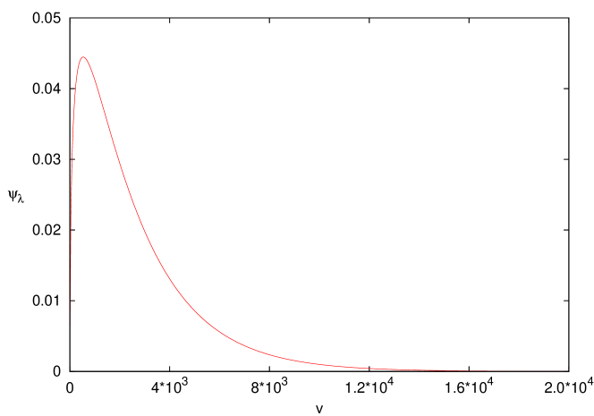
Figure 1: A normalizable eigenfunction $\psi_{\lambda}$ of the $\hat{\rho}$ operator defined via (72) corresponding to eigenvalue $\lambda>\rho_{{\rm cr}}$. An example presented here has eigenvalue very close to $\rho_{{\rm cr}}$, namely $(\lambda-\rho_{{\rm cr}})\approx 7.7\cdot 10^{-7}\rho_{{\rm cr}}$.

An important difficulty emerges in the case of $\Lambda>0$. Then, the scalar field energy density operator is not any longer non-negative in $\mathcal{H}_{\rm gr}$, because it is of the form

$$\hat{\rho}=-\vdots\frac{\rho_{{\rm cr}}}{8}B(v)^{\frac{1}{2}}(h_{-2}-h_{2})\tilde{A}(v)(h_{-2}-h_{2})B(v)^{\frac{1}{2}}\vdots\ -\ \Lambda\frac{1}{V_{o}}\hat{V}\hat{B}\ ,$$ (76)

and the essential part of its spectrum is shifted with respect to $\Lambda=0$ case by $-8\pi G\Lambda$. However, the solutions of the quantum constraint (86) take values in the subspace of $\mathcal{H}_{\rm gr}$ corresponding to the non-negative part of the spectrum of $\Theta$. The question (we do not know the answer to) is whether or not $\hat{\rho}$ restricted to that physical subspace becomes non-negative. Since the answer probably depends on the choice of the density operator, the non-negativity is a condition of the ordering in a definition of $\hat{\rho}$ consistent with the definition of $\Theta$.

VII Concluding remarks

The problem which we leave open is whether or not the quantum spacetime metric tensor operator should be uniquely defined in QG. The proposal of such construction was made in Section IV however it suffers the factor ordering ambiguity. At this point there are two aspects of that issue which are worth commenting.

First, the ordering ambiguity is restricted by the group averaging techniques. Since the starting point for that procedure is the kinematical Hilbert space, the operator $\hat{\pi}_{T}$ commutes with the geometry operators. Then the ambiguity is restricted just to a symmetrization of the product $\hat{\pi}_{T}\delta(\hat{T}-T_{0})$. We provide an extended explanation of that point in ga .

Second, it is possible to derive the propagation equation for a quantum test field on the quantum geometry background qft-qsp . Not surprisingly, the result involves the quantum metric tensor components. Remarkably, the expression is uniquely defined, whether the quantum metric tensor operator itself exists or not. Thus, the possible physical solution of that issue may be that the quantum metric is defined uniquely only through matter propagating on it.

Another unsolved issue is how to understand the space of solutions to the quantum scalar constraint corresponding to the lapse function $N=1$. The properties of each of the individual quantum constraint operators $\hat{C}(V)$ and, respectively, $\hat{C}(1)$ are familiar from the Schroedinger quantum mechanics. In the first case the classical trajectories are not complete in the evolution parameter, namely infinite volume is achieved in finite time. That is usually an indication that a self-adjoint extension is likely to be not unique. In the second case, the infinite volume is achieved only in infinite time. (The classical trajectories are incomplete at the zero volume as well, but in LQC this does not cause any evolution unbiguity.) Therefore there is the analogy with the quantum mechanics. The difference, and a new ambiguity is, that in gravity we can have two characteristics in a single theory depending on choice of the evolution parameter. The details of the construction of the solutions to the constraint operator $\hat{C}(1)$ from the solutions of the variuos extensions of the constraint operator $\hat{C}(V)$ will be presented in ga . Calculation of the partial observables might bring even more surprises.

Finally, in this work we have considered a simplest LQC model. However the full Quantum Gravity can be given a similar structure if it is formulated according to the Brown-Kuchar model BK ; GiesThiem-algiv . Therefore many results discussed in this paper is likely to admit generalizations to the full QG.

Appendix A Evolution operator in LQC: rigorous definition

In this appendix we present the completion of the definition of the symmetric evolution operator $\hat{\Theta}$ introduced in (31), taking special care of the difficulties related with either the vanishing

$$B(0)\ =\ 0$$ (77)

(in the case of $B=B_{\rm APS}$) or divergence

$$B(0)\ =\ \infty$$ (78)

(in the $B=B_{\rm sLQC}$ case).

Let us begin with (77). The operator $\hat{\Theta}$ has been well defined in Sec II in every subspace $\mathcal{H}_{\epsilon}\subset{\mathcal{H}_{{\rm gr},B}}$ and ${\epsilon\in(0,4)}$ through formula (31) already. The remaining case is $\epsilon=0$ (this problem is solved in aps-imp however it is not spelled out).

We start with a more suitable form of the constraint operator, namely we consider the solutions to the equation

$$-\frac{1}{2}\widehat{V^{-1}}\frac{\partial^{2}}{\partial T^{2}}\psi_{T}\ =\ \hat{C}_{\rm gr}\psi_{T},$$ (79)

where $\psi_{T}\in{\cal H}_{\rm gr}$ and the action of ${\widehat{C_{{\rm gr}}}}$ can be written (following (27)) as

$$[\hat{C}_{\rm gr}\psi_{T}](v)\ =\ C^{+}(v)\psi_{T}(v+4)+C^{o}(v)\psi_{T}(v)+C^{-}(v)\psi_{T}(v-4)\ ,$$ (80)

with $C^{o,\pm}(v)$ being real functions, of which $C^{o}(v)<0$.

Taking the scalar product of the left and the right hand sides respectively with the vector $|0\rangle\in{\mathcal{H}_{{\rm gr}}}$ we find

$$\langle 0|{\widehat{C_{{\rm gr}}}}\psi_{T}\rangle\ =\ 0\ .$$ (81)

This is a condition that has to be satisfied by $\psi_{T}\in{\mathcal{H}_{{\rm gr}}}$ at every value of $T$. The meaning of this observation is, that the functions $T\mapsto\psi_{T}\in{\mathcal{H}_{{\rm gr}}}$ which satisfy the constraint equation (79) in fact take values only in the subspace $\mathcal{H}_{\langle 0|{\widehat{C_{{\rm gr}}}}\cdot\rangle=0}$ defined by the constraint

$$\langle 0|{\widehat{C_{{\rm gr}}}}\psi\rangle\ =\ 0\ .$$ (82)

However the subspace is not preserved by ${\widehat{C_{{\rm gr}}}}$. It (the intersection of the domain ${\rm Span}(|v\rangle\ :\ v\in\mathbb{R})\cap\mathcal{H}_{\langle 0|{\widehat{C_{{\rm gr}}}}\cdot\rangle=0}$) is mapped into another subspace $\mathcal{H}_{\langle 0|\cdot\rangle=0}$ defined by the constraint

$$\langle 0|\psi\rangle\ =\ 0\ .$$ (83)

On the other hand, the orthogonal projection

$${\mathcal{H}_{{\rm gr}}}\ \rightarrow\ \mathcal{H}_{\langle 0|\cdot\rangle=0}$$ (84)

maps isometrically

$$\mathcal{H}_{\langle 0|\hat{C}_{\rm gr}\cdot\rangle=0}\ \rightarrow\ \mathcal{H}_{\langle 0|\cdot\rangle=0}\ .$$ (85)

This isomorphism can be used to push forward the operator ${\widehat{C_{{\rm gr}}}}$ to $\mathcal{H}_{\langle 0|\cdot\rangle=0}$. An action of the resulting operator (preserving $\mathcal{H}_{\langle 0|\cdot\rangle=0}$) is given by

$$[\hat{\tilde{C}}_{\rm gr}\psi](v)\ =\ \begin{cases}C^{+}(v)\psi(v+4)+C^{o}(v)\psi(v)+C^{-}(v)\psi(v-4)\ ,&v\not\in\{-4,0,4\}\ ,\\ \left\{\begin{split}&C^{+}(4)\psi(8)+C^{o}(4)\psi(4)\\ &-C^{-}(4)\left[\frac{C^{+}(0)}{C^{o}(0)}\psi(4)+\frac{C^{-}(0)}{C^{o}(0)}\psi(-4)\right]\end{split}\right\}\ ,&v=4\ ,\\ \qquad\qquad\qquad\qquad\quad 0\ ,&v=0\ ,\\ \left\{\begin{split}&C^{-}(-4)\psi(-8)+C^{o}(-4)\psi(-4)\\ &-C^{+}(-4)\left[\frac{C^{-}(0)}{C^{o}(0)}\psi(-4)+\frac{C^{+}(0)}{C^{o}(0)}\psi(4)\right]\end{split}\right\}\ ,&v=-4\ ,\\ \end{cases}\ .$$ (86)

It is worth to be stressed, that the Hilbert space isomorphism is not unitary in the kinematical Hilbert product, but it becomes unitary, after one endows the Hilbert space ${\cal H}_{\rm gr}$ with the $\langle\cdot|B\cdot\rangle$ product. Finally, the APS constraint is imposed on functions $T\mapsto\psi_{T}\in{\cal H}_{\langle 0|\cdot\rangle=0}={\cal H}_{{\rm gr},B}$ and it is

$$\partial^{2}_{T}\psi_{T}\ =\ 2V_{o}B(\hat{V})^{-1}\hat{\tilde{C}}_{\rm gr}{\psi}_{T}\ =:\ -2V_{o}\hat{\Theta}\psi_{T}\ .$$ (87)

This extends the definition of the operator $\hat{\Theta}$ given in the previous section to the subspace ${\cal H}_{\rm\epsilon=0}$ in the sub-domain

$${\rm Span}(|n\rangle\ \,:\,0\not=n\in 4\mathbb{Z})\ \subset{\cal H}_{\rm\epsilon=0}.$$

The operator $\hat{\Theta}$ is defined in the Hilbert space ${\cal H}_{{\rm gr},B}$ in the domain ${\rm Span}(|v\rangle\,:\,\mathbb{R})$ (however the zero volume vector $|0\rangle$ has zero norm in this space). It is a symmetric operator which may have inequivalent self-adjoint extensions (see section V), and one of them has to be chosen to make the quantum constraint equation well defined.

Exactly that method was used in the APS papers to study the physical solutions which take values in the subspace ${\cal H}_{\epsilon=0}$ (solutions preserved by the reflection $P|v\rangle=|-v\rangle$).

Let us turn now to the (78) case. Now the problem is in introducing the scalar product $\langle\cdot|B\cdot\rangle$. However instead, we can modify the procedure of going from (79) to an analog of (87) defining the operator

$$\hat{\Theta}\ :=\ -B(\hat{V})^{-1/2}{\widehat{C_{{\rm gr}}}}B(\hat{V})^{-1/2}\ ,$$ (88)

which is well defined and symmetric (in the domain ${\rm Span}(|v\rangle\ :\ v\in\mathbb{R})$) with respect to the original kinematical inner product of ${\mathcal{H}_{{\rm gr}}}$.

References

- (1) M. Bojowald, Loop Quantum Cosmology, Living Rev.Rel. 8, 11 (2005), arXiv: gr-qc/0601085.
- (2) A. Ashtekar, An Introduction to Loop Quantum Gravity Through Cosmology, Nuovo Cim. 122B, 135-155 (2007), arXiv: gr-qc/0702030.
-
(3)
C. Rovelli, Quantum Gravity (CUP, Cambridge, 2004);
A. Ashtekar and J. Lewandowski, Background Independent Quantum Gravity: A Status Report, Class.Quant.Grav. 21, R53 (2004), arXiv: gr-qc/0404018;
T. Thiemann, Introduction to Modern Canonical Quantum General Relativity (CUP, Cambridge, 2007). - (4) B. Bahr and T. Thiemann, Approximating the physical inner product of loop quantum cosmology, Class.Quant.Grav. 24 2109 (2007), arXiv: gr-qc/0607075.
- (5) W. Kamiński, J. Lewandowski, Ł. Szulc, The status of Quantum Geometry in the dynamical sector of Loop Quantum Cosmology, (2007), Class.Quant.Grav. 25 055003, arXiv: 0709.4225.
-
(6)
A. Ashtekar, T. Pawłowski and P. Singh, Quantum nature
of the big bang, Phys.Rev.Lett. 96, 141301 (2006),
arXiv: gr-qc/0602086;
A. Ashtekar, T. Pawłowski and P. Singh, Quantum nature of the big bang: An analytical and numerical investigation, Phys.Rev. D73, 124038 (2006), arXiv: gr-qc/0604013. - (7) A. Ashtekar, T. Pawłowski and P. Singh, Quantum nature of the big bang: Improved dynamics, Phys.Rev. D74, 084003 (2006), arXiv: gr-qc/0607039.
- (8) K. Giesel, T. Thiemann, Algebraic Quantum Gravity (AQG) IV. Reduced Phase Space Quantisation of Loop Quantum Gravity, arXiv: 0711.0119
- (9) A. Ashtekar, T. Pawłowski, P. Singh and K. Vandersloot, Loop quantum cosmology of FRW models, Phys.Rev. D75, 024035 (2007), arXiv: gr-qc/0612104.
- (10) Ł. Szulc, W. Kamiński and J. Lewandowski, Closed FRW model in Loop Quantum Cosmology, Class.Quant.Grav. 24, 2621-2635 (2007), arXiv: gr-qc/0612101.
-
(11)
K. Vandersloot, Loop quantum cosmology and the RW model,
Phys.Rev. D75, 023523 (2007),
arXiv: gr-qc/0612070;
Ł. Szulc, Open FRW model in Loop Quantum Cosmology, Class.Quant.Grav. 24, 6191-6200 (2007), arXiv: 0707.1816. -
(12)
A. Ashtekar, A. Corichi and P. Singh, Robustness of
key features of loop quantum cosmology,
Phys. Rev. D 77, 024046 (2008) arXiv: 0710.3565;
A. Corichi, P. Singh, Quantum bounce and cosmic recall, Phys. Rev. Lett. 100, 161302 (2008), arXiv: 0710.4543. - (13) W. Kamiński, J. Lewandowski, The flat FRW model in LQC: the self-adjointness, Class. Quantum Grav. 25 035001 (2008), arXiv: 0709.3120.
-
(14)
P. Singh, K. Vandersloot, Semi-classical States, Effective
Dynamics and Classical Emergence in Loop Quantum Cosmology,
Phys.Rev. D72, 084004 (2005), arXiv: gr-qc/0507029;
P. Singh, K. Vandersloot, G. V. Vereshchagin, Non-Singular Bouncing Universes in Loop Quantum Cosmology, Phys.Rev. D74, 043510 (2006), arXiv: gr-qc/0606032;
J. Mielczarek, T. Stachowiak, M. Szydłowski, Exact solutions for Big Bounce in loop quantum cosmology, (2008), arXiv: 0801.0502;
T. Cailleteau, A. Cardoso, K. Vandersloot, D. Wands, Singularities in loop quantum cosmology, (2008), arXiv: 0808.0190;
H. H. Xiong, T. Qiu, Y. F. Cai, X. Zhang, Cyclic Universe with Quintom matter in Loop Quantum Cosmology, (2007), arXiv: 0711.4469;
X. Fu, H. Yu, P. Wu, Dynamics of interacting phantom scalar field dark energy in Loop Quantum Cosmology, (2008), arXiv: 0808.1382. -
(15)
D. W. Chiou, Loop Quantum Cosmology in Bianchi Type I
Models: Analytical Investigation, Phys.Rev. D75, 024029
(2007), arXiv: gr-qc/0609029;
D. W. Chiou and K. Vandersloot, The behavior of non-linear anisotropies in bouncing Bianchi I models of loop quantum cosmology, Phys.Rev. D76, 084015 (2007), arXiv: 0707.2548;
D. W. Chiou, Effective Dynamics, Big Bounces and Scaling Symmetry in Bianchi Type I Loop Quantum Cosmology, Phys.Rev. D76, 124037 (2007), arXiv: 0710.0416;
Ł. Szulc, Loop Quantum Cosmology of Diagonal Bianchi Type I model: simplifications and scaling problems, Phys. Rev. D 78, 064035 (2008), arXiv: 0803.3559;
M. Martin-Benito, G. A. Mena-Marugan, T. Pawłowski, Loop Quantization of Vacuum Bianchi I Cosmology, Phys.Rev. D78, 064008 (2008), arXiv: 0804.3157. - (16) M. Artymowski, Z. Lalak, Ł. Szulc, Loop Quantum Cosmology corrections to inflationary models, (2008), arXiv: 0807.0160.
- (17) M. Martín-Benito, L. J. Garay and G. A. Mena Marugán, Hybrid Quantum Gowdy Cosmology: Combining Loop and Fock Quantization, Phys.Rev. D78, 083516 (2008), arXiv: 0804.1098.
-
(18)
M. Campiglia, R. Gambini and J. Pullin, Loop
quantization of spherically symmetric midi-superspaces,
Class.Quant.Grav. 24, 3649-3672 (2007),
arXiv: gr-qc/0703135;
R. Gambini, J. Pullin, Black holes in loop quantum gravity: the complete space-time, Phys.Rev.Lett. 101, 161301 (2008), arXiv: 0805.1187;
R. Gambini, J. Pullin, Diffeomorphism invariance in spherically symmetric loop quantum gravity, (2008), arXiv: 0807.4748. -
(19)
C. Rovelli, WHAT IS OBSERVABLE IN CLASSICAL AND QUANTUM GRAVITY?,
Class.Quant.Grav. 8 297 (1991);
C. Rovelli, Partial observables, Phys.Rev. D65 124013 (2002), arXiv: gr-qc/0110035;
B. Dittrich, Partial and complete observables for Hamiltonian constrained systems, Gen.Rel.Grav. 39 1891 (2007), arXiv: gr-qc/0411013;
B. Dittrich, Partial and Complete Observables for Canonical General Relativity, Class.Quant.Grav. 23 6155 (2006), arXiv: gr-qc/0507106;
T. Thiemann, Reduced phase space quantization and Dirac observables, Class.Quant.Grav. 23 1163 (2006), arXiv: gr-qc/0411031. - (20) A. Ashtekar, E. Wilson-Ewing, The covariant entropy bound and loop quantum cosmology (2008), arXiv: 0805.3511.
- (21) W. Kamiński, J. Lewandowski, T. Pawłowski, The physical states of LQC from the spectral decomposition of the scalar constraint for nonvanishing cosmological constant, in prep.
- (22) E. Bentivegna, T. Pawłowski, Anti-deSitter universe dynamics in LQC, Phys.Rev. D77, 124025 (2008), arXiv: 0803.4446.
- (23) A. Ashtekar, M. Bojowald, J. Lewandowski, Mathematical structure of loop quantum cosmology, Adv.Theo.Math.Phys. 7, 233-268 (2003), arXiv: gr-qc/0304074.
- (24) A. Ashtekar , T. Pawłowski, Loop quantum cosmology and the positive cosmological constant, in prep.
- (25) A. Ashtekar, W. Kamiński, J. Lewandowski, QFT in the expanding quantum spacetime in prep.
- (26) W. Kamiński, T. Pawłowski, The LQC evolution operator of FRW universe with positive cosmological constant, in prep.
-
(27)
D. Marolf, Refined algebraic quantization: Systems with a single
constraint, in Symplectic Singularities and Geometry of Gauge Fields
Banach Center Publications, Vol. 39 (1997), arXiv: gr-qc/9508015;
D. Marolf, Quantum observables and recollapsing dynamics, Class.Quant.Grav. 12, 1199-1220 (1995), arXiv: gr-qc/9404053;
D. Marolf, Observables and a Hilbert space for Bianchi IX, Class.Quant.Grav. 12, 1441-1454 (1995), arXiv: gr-qc/9409049;
D. Marolf, Almost ideal clocks in quantum cosmology: A brief derivation of time, Class.Quant.Grav. 12, 2469-2486 (1995), arXiv: gr-qc/9412016;
A. Ashtekar, J. Lewandowski, D. Marolf, J. Mourão and T. Thiemann, Quantization of diffeomorphism invariant theories of connections with local degrees of freedom, J.Math.Phys. 36, 6456-6493 (1995), arXiv: gr-qc/9504018. - (28) W. Kamiński, J. Lewandowski, T. Pawłowski, The evolution and the constraint operators in LQC In prep.
-
(29)
B. Simon, Classical moment problem as a
self-adjoint finite difference operator, arXiv: math-ph:9906008;
G. Teschl, Jacobi operators and completely integrable nonlinear lattices, Mathematical surveys and monographs 72, Amer. Math. Soc., Providence, (2000). - (30) J.D. Brown, K.V. Kuchar, Dust as a Standard of Space and Time in Canonical Quantum Gravity, Phys.Rev. D51 5600-5629 (1995), arXiv: gr-qc/9409001