Conductivity of suspended and non-suspended graphene at finite gate voltage

Abstract

We compute the DC and the optical conductivity of graphene for finite values of the chemical potential by taking into account the effect of disorder, due to mid-gap states (unitary scatterers) and charged impurities, and the effect of both optical and acoustic phonons. The disorder due to mid-gap states is treated in the coherent potential approximation (CPA, a self-consistent approach based on the Dyson equation), whereas that due to charged impurities is also treated via the Dyson equation, with the self-energy computed using second order perturbation theory. The effect of the phonons is also included via the Dyson equation, with the self energy computed using first order perturbation theory. The self-energy due to phonons is computed both using the bare electronic Green’s function and the full electronic Green’s function, although we show that the effect of disorder on the phonon-propagator is negligible. Our results are in qualitative agreement with recent experiments. Quantitative agreement could be obtained if one assumes water molelcules under the graphene substrate. We also comment on the electron-hole asymmetry observed in the DC conductivity of suspended graphene.

I Introduction

The isolation of a single carbon layer via micromechanical cleavage has triggered immense research activity.pnas Apart from the anomalous quantum Hall effect due to chiral Dirac-like quasi-particles,Nov05 ; Kim05 the finite “universal” DC conductivity at the neutrality point attracted major attention.Nov04 For recent reviews see Refs. Nov07, ; Katsnelson07, ; peresworld, ; GeimPhysToday, ; rmp, ; rmpBeenakker, .

The electronic properties of graphene are characterized by two nonequivalent Fermi-surfaces around the $K$ and $K^{\prime}$-points, respectively, which shrink to two points at the neutrality point $\mu=0$ ($\mu$ is chemical potential). The spectrum around these two points is given by an (almost) isotropic energy dispersion $E({\bm{k}})=\pm v_{F}\hbar k$ with the Fermi velocity $v_{F}\simeq 10^{6}$ m/s.Wallace Graphene can thus be described by an effective (2+1)-dimensional relativistic field theory with the velocity of light $c$ replaced by the Fermi velocity $v_{F}$.Semenoff84

Relativistic field theories in (2+1) dimensions were investigated long before the actual discovery of grapheneHaldane88 ; Ludwig94 and also the two values of the universal conductivities of a clean system at the neutrality point depending on whether one includes a broadening $\Gamma\rightarrow 0$ or not were reported then.Ryu06 ; Ziegler07 ; GusyninIJMPB In the first case, one obtains $\sigma_{\Gamma\rightarrow 0}^{\mu=0}=\frac{4}{\pi}e^{2}/h$,Gorbar02 the second case yields $\sigma_{\Gamma=0}^{\mu=0}=\frac{\pi}{2}e^{2}/h$.Falkovsky07 Interestingly, the first value is also obtained without the limit $\Gamma\rightarrow 0$ within the self-consistent coherent potential approximation (CPA).PeresPRB We also note that the constant conductivity holds for zero temperature, only; for finite temperature the DC conductivity is zero.PeresIJMPB

If leads are attached to the graphene sample, an external broadening is introduced and the conductivity is given by $\sigma_{\Gamma\rightarrow 0}^{\mu=0}$ Katsnelson06 ; Beenakker06 ; Verges07 which has been experimentally verified for samples with large aspect ratio.Lau07 This is in contrast to measurements of the optical conductivity, where leads are absent and a finite energy scale given by the frequency $\omega$ of the incoming beam renders the intrinsic disorder negligible, $\Gamma/\hbar\omega\approx 0$. One thus expects the universal conductivity to be given by $\sigma_{\Gamma=0}^{\mu=0}=\frac{\pi}{2}e^{2}/h$, which was measured in various experiments in graphene on a SiO₂,Basov SiC-substrateGeorge and free hanging.GeimOptics Also in graphene bilayer and multilayers,George ; GeimOptics as well as in graphiteKuzmenko the conductivity per plane is of the order of $\sigma_{0}\equiv\frac{\pi}{2}e^{2}/h$.

The above results were obtained from the Kubo or Laundauer formula and assumed coherent transport. Also diffusive models based on the semi-classical Boltzmann approach yield a finite DC conductivity at the neutrality point. Nevertheless, the finite conductivity was found to be non-universalNomura06 ; Adam07 ; PeresBZ ; StauberBZ ; Kim07 in contraditions to the findings of early experiments, which suggested $\sigma_{\rm min}\approx 4e^{2}/h$.Nov04 We should however stress that one can still assume a certain degree of universality, since the experimental values for the conductivity are all of the order of $4e^{2}/h$. It was argued that electron-hole puddlesCheianov07 or potential fluctuations in the substrateAdam07 can account for a finite conductivity at the Dirac point. An alternative explanation of this quasi-universal behavior seen in experiments is that there is only a logarithmic dependence on the impurity concentration due to mid-gap states and therefore only in cleaner samples deviations from the universal value are seen.StauberBZ

On the other hand, the optical conductivity is given by the universal conductivity $\sigma_{0}$ for frequencies larger than twice the chemical potential $\mu$. It is remarkable that this universal value also holds in the optical frequency range,GeimOptics ; Stauber08 a result with important consequences in applications.ap1 ; ap2 ; ap3 Only for frequencies $\hbar\omega<2\mu$, the sample-dependent scattering behavior of the electrons becomes important and recent experiments in show an decay of the universal conductivity with unusual large broadening around $2\mu$ which can not be explained by thermal effects.Basov Moreover, the spectral weight for $k_{B}T\ll\hbar\omega\ll 2\mu$ does not reach zero as would be expected due to Pauli blocking, but assumes an almost constant plateau of $\sigma\approx\sigma_{0}/3$ for larger gate voltage.

The first calculations of the optical conductivity of graphene, using the Dirac Hamiltonian were done in Ref. [PeresPRB, ]. This study was subsequently revisited a number of times, Gusynin06PRL ; Gusynin07PRL ; Gusynin07 and summarized in Ref. [GusyninIJMPB, ]. In these calculations the effect of disorder was treated in a phenomenological manner, by broadening the delta functions into Lorentzians characterized by constant width $\Gamma$. As shown in Ref. [PeresPRB, ] however, the momentum states are non-uniformly broadened, with the states close to the Dirac point being much more affected by the impurities than those far away from that point. In the clean limit, the exact calculation of the optical properties of graphene was considered in Ref. [Pedersen, ], a calculation recently generalized to the calculation of the optical properties of graphene antidot lattices.pedersen2

In this paper, we generalize the results of Ref. [PeresPRB, ] by considering a finite chemical potential, including the effect of charge impurities, and the scattering by phonons. We discuss two main corrections to the clean system and calculate the optical conductivity. First, we include the coupling of the Dirac fermions to in-plane phonons, acoustical as well as optical ones. Out-of-plane phonons only have a negligible effect on the electronic properties of graphene.StauberHolstein08 Secondly, we include various types of disorder which give rise to mid-gap states as well as Coulomb scatterers.

In Sec. II, we define the phonon Hamiltonian, deduce the electron-phonon interaction and calculate the electronic self-energy. In Sec. III.1, we discuss the Green’s function which is modified due to impurities and phonons. We then present our results for DC and optical conductivity and compare it to the experiment of Ref. [Basov, ]. We close with remarks and conclusions.

II Electrons and Phonons

II.1 Tight-binding Hamiltonian and current operator

The Hamiltonian, in tight binding form, for electrons in graphene is written as

$$H = -\sum_{\bm{R},\sigma}\sum_{\bm{\delta}}t(\bm{R},\bm{R}+\bm{\delta})[a^{\dagger}_{\sigma}(\bm{R})b_{\sigma}(\bm{R}+\bm{\delta})+H.c.]$$ (1)

where the operator $a^{\dagger}_{\sigma}(\bm{R})$ creates an electron in the carbon atoms of sub-lattice $A$, and $b^{\dagger}_{\sigma}(\bm{R})$ does the same in sub-lattice $B$. The hopping parameter, $t(\bm{R},\bm{R}+\bm{\delta})$, depends on the relative position of the carbon atoms both due to the presence of a vector potential $\bm{A}(t)$ and due to the vibration of the carbon atoms. The vectors $\bm{\delta}$ have the form

$$\begin{array}[]{l}\displaystyle{\bm{\delta}_{1}=\frac{a}{2}\left(1,\sqrt{3}\right)\qquad\bm{\delta}_{2}=\frac{a}{2}\left(1,-\sqrt{3}\right)\qquad\bm{\delta}_{3}=-a\left(1,0\right)}\,,\end{array}$$ (2)

where $a$ is the carbon-carbon distance. In order to obtain the current operator we write the hopping parameter as

$$t\rightarrow te^{i(e/\hbar)\bm{A}(t)\cdot\bm{\delta}}\,.$$ (3)

Expanding the exponential up to second order in the vector potential $\bm{A}(t)$,and assuming that the electric field is oriented along the $x$ direction, the current operator is obtained from

$$j_{x}=-\frac{\partial H}{\partial A_{x}(t)}\,,$$ (4)

leading to $j_{x}=j_{x}^{P}+A_{x}(t)j^{D}_{x}$. The operator $j_{x}^{P}$ reads

$$j_{x}^{P} = \frac{tie}{\hbar}\sum_{\bm{R},\sigma}\sum_{\bm{\delta}}[\delta_{x}a^{\dagger}_{\sigma}(\bm{R})b_{\sigma}(\bm{R}+\bm{\delta})-H.c.]\,.$$ (5)

The current term of the operator proportional to $A_{x}(t)$ will not be used in this paper, and therefore it is pointless to give its form here.Stauber08 ; PeresIJMPB

II.2 Phonon modes

In order to describe the effect of phonons in graphene we adopt the model developed by Woods and MahanWoods and extensively used by other authors.Suzuura ; Ando06 ; Ishikawa ; Neto The potential energy of the model is a sum of two terms. The first is due to bond-stretching and reads

$$V_{1}=\frac{\alpha}{2}\sum_{\bm{R}}\sum_{\delta}[\bm{u}_{A}(\bm{R})-u_{B}(\bm{R}+\bm{\delta})\cdot\bm{\delta}/a]^{2}\,,$$ (6)

where $u_{A}(\bm{R})$ and $u_{B}(\bm{R}+\bm{\delta})$ represent the small displacements relatively to the equilibrium position of the carbon atoms in the sub-lattice $A$ and sub-lattice $B$, respectively. If only the term (6) is used a simple analytical expression for the eigen-modes is obtained.Cserti The second term of the model is due to angle deformation and has the form

$$V_{2} = \frac{\beta}{2a^{4}}\sum_{\bm{R}}\left\{[(\bm{\delta}_{1}/2+\bm{\delta}_{2})\cdot(\bm{u}_{A}(\bm{R})-\bm{u}_{B}(\bm{R}+\bm{\delta}_{1}))+(\bm{\delta}_{2}/2+\bm{\delta}_{1})\cdot(\bm{u}_{A}(\bm{R})-\bm{u}_{B}(\bm{R}+\bm{\delta}_{2}))]^{2}\right.$$ (7)

$$+ [(\bm{\delta}_{1}/2+\bm{\delta}_{3})\cdot(\bm{u}_{A}(\bm{R})-\bm{u}_{B}(\bm{R}+\bm{\delta}_{1}))+(\bm{\delta}_{3}/2+\bm{\delta}_{1})\cdot(\bm{u}_{A}(\bm{R})-\bm{u}_{B}(\bm{R}+\bm{\delta}_{3}))]^{2}$$

$$+ [(\bm{\delta}_{2}/2+\bm{\delta}_{3})\cdot(\bm{u}_{A}(\bm{R})-\bm{u}_{B}(\bm{R}+\bm{\delta}_{2}))+(\bm{\delta}_{3}/2+\bm{\delta}_{2})\cdot(\bm{u}_{A}(\bm{R})-\bm{u}_{B}(\bm{R}+\bm{\delta}_{3}))]^{2}$$

$$+ [(\bm{\delta}_{1}/2+\bm{\delta}_{2})\cdot(\bm{u}_{B}(\bm{R}+\bm{\delta}_{3})-\bm{u}_{A}(\bm{R}-\bm{a}_{1}))+(\bm{\delta}_{2}/2+\bm{\delta}_{1})\cdot(\bm{u}_{B}(\bm{R}+\bm{\delta}_{3})-\bm{u}_{A}(\bm{R}-\bm{a}_{2}))]^{2}$$

$$+ [(\bm{\delta}_{1}/2+\bm{\delta}_{3})\cdot(\bm{u}_{B}(\bm{R}+\bm{\delta}_{3})-\bm{u}_{A}(\bm{R}-\bm{a}_{1}))+(\bm{\delta}_{3}/2+\bm{\delta}_{1})\cdot(\bm{u}_{B}(\bm{R}+\bm{\delta}_{3})-\bm{u}_{A}(\bm{R}))]^{2}$$

$$+ \left.[(\bm{\delta}_{2}/2+\bm{\delta}_{3})\cdot(\bm{u}_{B}(\bm{R}+\bm{\delta}_{3})-\bm{u}_{A}(\bm{R}-\bm{a}_{2}))+(\bm{\delta}_{3}/2+\bm{\delta}_{2})\cdot(\bm{u}_{B}(\bm{R}+\bm{\delta}_{3})-\bm{u}_{A}(\bm{R}))]^{2}\right\}\,,$$

where $\bm{a}_{1}=\bm{\delta}_{1}-\bm{\delta}_{3}$ and $\bm{a}_{2}=\bm{\delta}_{2}-\bm{\delta}_{3}$, represent the vectors defining the unit cell. The kinetic energy has the form

$$T=\sum_{\bm{R}}\frac{M_{C}}{2}[\dot{\bm{u}}_{A}(\bm{R})]^{2}+\frac{M_{C}}{2}[\dot{\bm{u}}_{B}(\bm{R})]^{2}\,,$$ (8)

where $M_{C}$ is the Carbon atom mass. The Lagrangian $L=T-V_{1}-V_{2}$ leads to an eigenproblem of the form $M\omega^{2}\bm{w}=\bm{D}\bm{w}$, where

$$\bm{w}=\left(\begin{array}[]{c}u_{Ax}\\ u_{Ay}\\ u_{Bx}\\ u_{By}\end{array}\right)\,,$$ (9)

and $\bm{D}$ is the dynamical matrix reading

$$\bm{D}=\left(\begin{array}[]{cccc}X_{1}&F&A&C\\ F^{\ast}&X_{2}&C&B\\ A^{\ast}&C^{\ast}&X_{1}&F\\ C^{\ast}&B^{\ast}&F&X_{2}\end{array}\right)\,,$$ (10)

with

$$X_{1} = \frac{3}{2}\alpha+\frac{45}{8}\beta+\frac{9}{8}\beta\cos(\sqrt{3}Q_{y}a)\,,$$ (11)

$$X_{2} = \frac{2}{3}\alpha+\frac{45}{8}\beta-\frac{3}{8}\beta\cos(\sqrt{3}Q_{y}a)$$ (12)

$$+ \frac{3}{2}\beta\cos(3Q_{x}a/2)\cos(\sqrt{3}Q_{y}a/2)\,,$$

$$A = -\alpha e^{-iQ_{x}a}-\left(\frac{\alpha}{2}+\frac{27}{4}\beta\right)\cos(\sqrt{3}Q_{y}a/2)e^{iQ_{x}a/2}\,,$$ (13)

$$B = -\frac{9}{2}\beta e^{-iQ_{x}a}-\left(\frac{3}{2}\alpha+\frac{9}{4}\beta\right)\cos(\sqrt{3}Q_{y}a/2)e^{iQ_{x}a/2}\,,$$ (14)

$$C = -i\sqrt{3}\left(\frac{\alpha}{2}-\frac{9}{4}\beta\right)\sin(\sqrt{3}Q_{y}a/2)e^{iQ_{x}a/2}\,,$$ (15)

$$F = i\beta\frac{3\sqrt{3}}{8}[\sin(\sqrt{3}Q_{y}a)-2\sin(\sqrt{3}Q_{y}/2)e^{i3Q_{x}a/2}]\,,$$ (16)

where we have redefined $\beta$ as $\beta/a^{2}$ and $\bm{Q}=(Q_{x},Q_{y})$ is the momentum of the excitation. This model can be diagonalized numerically and its spectrum is represented in Fig. 1.

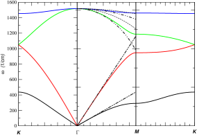
Figure 1: (color online) Phonon spectrum of the honeycomb lattice, using $\alpha=500$ N/m and $\beta=10$ N/m, such that the optical frequency at the $\Gamma$-point is or the order of 1600 cm^-1. Also shown are the spectra of the simplified model discussed in the text (dashed lines) and the effective model discussed in Appendix A (dashed-dotted lines).

Although this model can easily be solved numerically, it is useful to derive from it a simple analytical model which helps in the analytical calculation of the electron-phonon problem. To do so, we follow Suzuura and AndoSuzuura and introduce two effective models, one for the acoustic and the other for the optical excitations, associated with the fields $\bm{u}=(\bm{u}_{A}+\bm{u}_{B})/\sqrt{2}$ and $\bm{v}=(\bm{u}_{A}-\bm{u}_{B})/\sqrt{2}$, respectively. The effective Hamiltonian for the acoustic modes has the form

$$H=K_{1}a^{2}\left(\begin{array}[]{cc}Q^{2}_{x}&Q_{x}Q_{y}\\ Q_{x}Q_{y}&Q^{2}_{y}\end{array}\right)+K_{2}a^{2}\left(\begin{array}[]{cc}Q^{2}_{x}+Q^{2}_{y}&0\\ 0&Q^{2}_{x}+Q^{2}_{y}\end{array}\right)\,,$$ (18)

with $K_{1}=3\alpha/8$ and $K_{2}=27\alpha\beta/(8\alpha+36\beta/2)$. The eigenmodes of this effective Hamiltonian are

$$M_{C}\omega^{2}=K_{2}(Qa)^{2}\,,$$ (19)

and

$$M_{C}\omega^{2}=(K_{2}+K1)(Qa)^{2}\,,$$ (20)

with polarization vectors

$$\bm{\epsilon}_{TA}=i(-Q_{y},Q_{x})/Q\,,$$ (21)

and

$$\bm{\epsilon}_{LA}=i(Q_{x},Q_{y})/Q\,,$$ (22)

respectively. The velocity of the modes is given by

$$v_{TA}=a\sqrt{K_{2}/M_{C}}\,,$$ (23)

and

$$v_{LA}=a\sqrt{(K_{1}+K_{2})/M_{C}}\,.$$ (24)

The eigenmodes (19) and (20) are represented in Fig. 1 by dashed lines. They cannot be distinguished from the effective model described in Appendix A. The effective Hamiltonian for the optical modes is given by

$$H = K_{0}\left(\begin{array}[]{cc}1&0\\ 0&1\end{array}\right)-K_{3}a^{2}\left(\begin{array}[]{cc}Q^{2}_{x}&Q_{x}Q_{y}\\ Q_{x}Q_{y}&Q^{2}_{y}\end{array}\right)$$ (29)

$$- K_{4}a^{2}\left(\begin{array}[]{cc}Q^{2}_{x}+Q^{2}_{y}&0\\ 0&Q^{2}_{x}+Q^{2}_{y}\end{array}\right)\,,$$ (32)

with $K_{0}=3(\alpha+9\beta/2)$, $K_{3}=(3\alpha/8-27\beta/8)$, and $K_{4}=27\beta(\alpha+9/4\beta)/(8\alpha+36\beta)$. The eigenmodes are

$$M_{C}\omega^{2}=K_{0}-K_{4}(Qa)^{2}\,,$$ (33)

and

$$M_{C}\omega^{2}=K_{0}-(K_{3}+K_{4})(Qa)^{2}\,,$$ (34)

with polarization vectors given by

$$\bm{\epsilon}_{TO}=i(-Q_{y},Q_{x})/Q\,,$$ (35)

and

$$\bm{\epsilon}_{LO}=i(Q_{x},Q_{y})/Q\,,$$ (36)

respectively. The modes (33) and (34) are represented in Fig. (1) by dashed lines. The dashed-dotted lines of the same Figure are derived from an effective model, discussed in Appendix A.

II.3 Electron-phonon interaction

We now address the question of the electron-phonon interaction. This comes about because the hopping $t$ depends on the absolute distance between neighboring carbon atoms. We therefore have

$$t[a+(\bm{u}_{A}(\bm{R})-\bm{u}_{B}(\bm{R}+\bm{\delta}))\cdot\bm{\delta}/a]\simeq t[a]$$ (37)

$$+ \frac{1}{a}\frac{\partial t[a]}{\partial a}(\bm{u}_{A}(\bm{R})-\bm{u}_{B}(\bm{R}+\bm{\delta}))\cdot\bm{\delta}\,.$$

Replacing (37) in the Hamiltonian (1) and introducing the Fourier representation

$$a_{\sigma}(\bm{R})=\frac{1}{\sqrt{N}_{c}}\sum_{\bm{k}}e^{i\bm{k}\cdot\bm{R}}a_{\sigma}(\bm{k})\,,$$ (38)

and

$$u_{A}(\bm{R})=\frac{1}{\sqrt{N}_{c}}\sum_{\bm{Q}}e^{i\bm{Q}\cdot\bm{R}}u_{A}(\bm{Q})\,,$$ (39)

with similar equations for $b_{\sigma}(\bm{R})$ and $u_{B}(\bm{R})$, the electron-phonon interaction has form

$$H_{e-ph} = -\frac{1}{a}\frac{\partial t}{\partial a}\frac{1}{\sqrt{N}_{c}}\sum_{\bm{Q},\bm{k}}\sum_{\sigma,\bm{\delta}}[\bm{u}_{A}(\bm{Q})-\bm{u}_{B}(\bm{Q})e^{i\bm{Q}\cdot\bm{\delta}}]\cdot\bm{\delta}$$ (40)

$$\times [e^{i\bm{k}\cdot\bm{\delta}}a^{\dagger}_{\sigma}(\bm{k}+\bm{Q})b_{\sigma}(\bm{k})+e^{-i\bm{k}\cdot\bm{\delta}}b^{\dagger}_{\sigma}(\bm{k})a_{\sigma}(\bm{k}-\bm{Q})]\,.$$

Since we are interested in the effect of the phonons with momentum close to the $\Gamma$-point, the phase $e^{i\bm{Q}\cdot\bm{\delta}}$ is expanded as $e^{i\bm{Q}\cdot\bm{\delta}}\simeq 1-i\bm{Q}\cdot\bm{\delta}$. Introducing the optical modes $\bm{v}$, the electron-phonon interaction with the optical phonon modes has the form

$$H_{e-ph}^{opt} = -\frac{1}{a}\frac{\partial t}{\partial a}\frac{1}{\sqrt{N}_{c}}\sum_{\bm{Q},\bm{k}}\sum_{\sigma,\nu,\bm{\delta}}\sqrt{\frac{\hbar}{M_{C}\omega_{\nu}(\bm{Q})}}\bm{\epsilon}_{\nu}(\bm{Q})\cdot\bm{\delta}$$ (41)

$$\times (B^{\dagger}_{-\bm{Q},\nu}+B_{\bm{Q},\nu})[e^{i\bm{k}\cdot\bm{\delta}}a^{\dagger}_{\sigma}(\bm{k}+\bm{Q})b_{\sigma}(\bm{k})$$

$$+ e^{-i\bm{k}\cdot\bm{\delta}}b^{\dagger}_{\sigma}(\bm{k})a_{\sigma}(\bm{k}-\bm{Q})]\,.$$

Introducing the acoustic modes $\bm{u}$, the electron-phonon interaction with the acoustic phonon modes has the form

$$H_{e-ph}^{ac} = \frac{i}{a}\frac{\partial t}{\partial a}\frac{1}{\sqrt{N}_{c}}\sum_{\bm{Q},\bm{k}}\sum_{\sigma,\nu,\bm{\delta}}\sqrt{\frac{\hbar}{4M_{C}\omega_{\nu}(\bm{Q})}}(\bm{\epsilon}_{\nu}(\bm{Q})\cdot\bm{\delta})$$ (42)

$$\times (\bm{Q}\cdot\bm{\delta})(B^{\dagger}_{-\bm{Q},\nu}+B_{\bm{Q},\nu})[e^{i\bm{k}\cdot\bm{\delta}}a^{\dagger}_{\sigma}(\bm{k}+\bm{Q})b_{\sigma}(\bm{k})$$

$$+ e^{-i\bm{k}\cdot\bm{\delta}}b^{\dagger}_{\sigma}(\bm{k})a_{\sigma}(\bm{k}-\bm{Q})]\,.$$

In both Eqs. (41) and (42) the $B_{\bm{Q},\nu}(B^{\dagger}_{\bm{Q},\nu})$ operators are destruction (creation) operators of phonons of momentum $\bm{Q}$ and polarization $\nu$.

III Electronic Green’s function

The electronic Green’s function in the Dirac cone approximation has the form

$$\mathbbm{G}=\frac{\left(\begin{array}[]{cc}i\omega_{n}-\Sigma(i\omega_{n})&-t\phi(\bm{k})\\ -t\phi^{\ast}(\bm{k})&i\omega_{n}-\Sigma(i\omega_{n})\end{array}\right)}{[i\omega_{n}-\Sigma(i\omega_{n})][i\omega_{n}-\Sigma(i\omega_{n})]-t^{2}|\phi(\bm{k})|^{2}}\,,$$ (43)

with $\phi(\bm{k})=\sum_{\bm{\delta}}e^{i{\bm{k}}\cdot{\bm{\delta}}}$. The electronic self-energy shall be given by

$$\Sigma(i\omega_{n})=\Sigma^{imp}(\bm{K},i\omega_{n})+\Sigma^{pho}(\bm{K},i\omega_{n})\,,$$ (44)

where $\Sigma_{imp}(\bm{K},i\omega_{n})=\Sigma_{unit}(i\omega_{n})+\Sigma_{Coul}(\bm{K},i\omega_{n})$ represents the contribution due to mid-gap states (unitary scatterers) as well as long-range Coulomb scatterers. The self-energy $\Sigma_{pho}(\bm{K},i\omega_{n})=\Sigma_{opt}(\bm{K},i\omega_{n})+\Sigma_{ac}(\bm{K},i\omega_{n})$ represents the contributions due to optical and acoustic phonons. We note that the self-energies originating from the electron-phonon and Coulomb interaction are evaluated at the Dirac momentum $\bm{K}=2\pi(1/3,\sqrt{3}/9)/a$. In the following, we will discuss the Green’s functions due to the the various contributions.

III.1 Green’s function with mid-gap states (unitary scatterers)

The physical origin of mid-gap states in the spectrum of graphene is varied. Cracks, edges, vacanciesUrsel are all possible sources for mid-gap states. From an analytical point of view, these types of impurities (scatterers) are easily modeled by considering the effect of vacancies. We stress, however, that this route is chosen due to its analytic simplicity.

The effect of mid-gap states on the conductivity of graphene was first considered by Peres et al. PeresPRB for the case a half-filled system. Considering the effect of a local scattering potential of intensity $\epsilon_{0}$, the Green’s function has the form of Eq. (43) with the retarded self-energy

$$\Sigma_{unit}^{ret}(\omega)=\frac{n_{i}\epsilon_{0}}{\hbar}\frac{1-\epsilon_{0}F(\omega)-i\epsilon_{0}\pi R(\omega)}{[1-\epsilon_{0}F(\omega)]^{2}+[\epsilon_{0}\pi R(\omega)]^{2}}\,,$$ (45)

where the functions $F(\omega)$ and $R(\omega)$ are defined by

$$\frac{1}{\hbar N_{c}}\sum_{\bm{k}}G(\bm{k},\omega+i0^{+})=F(\omega)-i\pi R(\omega)\,.$$ (46)

Mid-gap states are obtained by making the limit $\epsilon_{0}\rightarrow\infty$, which resembles the unitary limit. Clearly, $R(\omega)$ is the density of states per spin per unit cell. Let us write $\Sigma_{unit.}^{ret}(\omega)$ as a sum of real and imaginary parts, $\Sigma_{unit}^{ret}(\omega)=\Sigma^{\prime}(\omega)+i\Sigma^{\prime\prime}(\omega)$ (note that $\Sigma^{\prime\prime}>0$). The functions $F(\omega)$ and $R(\omega)$ are determined self-consistently through the numerical solution of the following set of equations:

$$F(\omega)-i\pi R(\omega)=\frac{1}{t^{2}\pi\sqrt{3}}[\hbar\Sigma^{\prime\prime}(\Upsilon-i\Psi/2)$$

$$+(\hbar\omega-\hbar\Sigma^{\prime})(\Psi/2-i\Upsilon)]\,,$$ (47)

with $\Upsilon$ and $\Psi$ given by

$$\Upsilon=\sum_{\alpha=\pm 1}-\arctan\frac{\hbar\Sigma^{\prime}-\omega\hbar}{\hbar\Sigma^{\prime\prime}}+\arctan\frac{\hbar\Sigma^{\prime}-\omega\hbar+\alpha D}{\hbar\Sigma^{\prime\prime}}\,,$$ (48)

and

$$\Psi=\sum_{\alpha=\pm 1}\log\frac{(\hbar\Sigma^{\prime\prime})^{2}+(\hbar\Sigma^{\prime}-\hbar\omega)^{2}}{(\hbar\Sigma^{\prime\prime})^{2}+(\hbar\Sigma^{\prime}-\hbar\omega+\alpha D)^{2}}\,.$$ (49)

In Figure 2, we compare the density of states computed using the coherent potential approximation (CPA) equations with that obtained from a numerical exact method. vitorprl It is clear that the CPA captures the formation of mid-gap states in a quantitative way. The main difference is the presence of a peak at zero energy in the exact density of states, whose measure is quantitatively negligible.

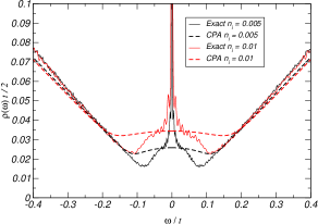
Figure 2: (color online) Density of states of graphene in the presence of mid-gap states. The CPA calculation is compared with a numerical exact method. The concentration of impurities is $n_{i}=0.005$ and $n_{i}=0.01$. Here and in the following figures we use $t=3$ eV and a cutoff energy of $D=7$ eV.

In Figure 3 we depict the self-energy calculation using the CPA equations, for two different values of the impurity concentration. It is clear that $\Sigma^{\prime\prime}(\omega)$ increases close to zero energy leading to a broadening of the electronic states close to the Dirac point.

Figure 3: (color online) CPA calculation of the self-energy $\hbar\Sigma_{unit}^{ret}(\omega)$ for two impurity concentrations, $n_{i}=0.001$ and $n_{i}=0.0005$. The left panel shows the imaginary part and the right one shows the real part of the self-energy.

III.2 Green’s function with Coulomb impurities

It has been argued that charged impurities are crucial to understand the transport properties of graphene on top of a silicon oxide substrate.Nomura ; Adam07 ; Chen In what follows, we compute the electronic self-energy due to charge impurities, using second order perturbation theory in the scattering potential. Electronic scattering from an impurity of charge $Ze$ leads to a term in the Hamiltonian of the form

$$V=-\sum_{\bm{R},\sigma}\frac{Ze^{2}}{\sqrt{d^{2}+\bm{R}^{2}}}[a^{\dagger}_{\sigma}(\bm{R})a_{\sigma}(\bm{R})+b^{\dagger}_{\sigma}(\bm{R})b_{\sigma}(\bm{R})]\,.$$ (50)

In momentum space $V$ reads

$$V=\frac{1}{N_{c}}\sum_{\bm{p},\bm{q},\sigma}V_{0}(\bm{q})[a^{\dagger}_{\sigma}(\bm{p})a_{\sigma}(\bm{p}+\bm{q})+b^{\dagger}_{\sigma}(\bm{p})b_{\sigma}(\bm{p}+\bm{q})],$$ (51)

where $V_{0}(\bm{q})$ reads

$$V_{0}(\bm{q})=-\sum_{\bm{R}}\frac{Ze^{2}e^{i\bm{R}\cdot\bm{q}}}{\sqrt{d^{2}+\bm{R}^{2}}}\,.$$ (52)

With $\mathbbm{G}^{0}(\bm{k},i\omega_{n})$ the bare and $\mathbbm{G}(\bm{k},\bm{p},i\omega_{n})$ the full Green’s functions, the Dyson equation due to one Coulomb impurity reads

$$\mathbbm{G}(\bm{k},\bm{p},\omega_{n}) = \delta_{\bm{k},\bm{p}}+\mathbbm{G}^{0}(\bm{k},i\omega_{n})$$ (53)

$$\times \frac{1}{\hbar N_{c}}\sum_{\bm{k}^{\prime}}V_{0}(\bm{k}-\bm{k}^{\prime})\mathbbm{G}(\bm{k}^{\prime},\bm{p},\omega_{n})\;.$$

If we consider a finite density per unit cell, $n^{C}_{i}$, and incoherent scattering between impurities, the second-order self-energy is given by

$$\Sigma_{Coul}^{ret}(\bm{k},i\omega_{n})=\frac{n^{C}_{i}}{\hbar^{2}N_{c}}\sum_{\bm{p}}V^{2}(\bm{k}-\bm{p})\mathbbm{G}^{0}(\bm{p},i\omega_{n})\,,$$ (54)

where a term of the form $n^{C}_{i}V(0)/\hbar$ was absorbed in the chemical potential, since it corresponds to an energy shift only. Note that we have replaced $V_{0}(\bm{q})$ by $V(\bm{q})$, which corresponds to include the effect of electronic screening in the calculation. The form of $V(\bm{q})$ is (in S.I. units)StauberBZ

$$V(\bm{q})=-\frac{Ze^{2}}{2\epsilon_{0}\epsilon A_{c}}\frac{e^{-qd}}{q+\gamma}\,,$$ (55)

where $\epsilon=3.9$ is the Silicon Oxide relative permittivity, $d$ is the distance from the charge to the graphene plane, and $\gamma$ is given by

$$\gamma=\frac{\rho(\mu)e^{2}}{2\epsilon_{0}\epsilon A_{c}}\,,$$ (56)

where $\rho(\mu)$ is the self-consistent density of states as computed from the CPA calculation ($A_{c}=3\sqrt{3}a^{2}/2$ is the area of the unit cell).

The self-energy (54) is dependent both on the momentum $\bm{k}$ and on the frequency. However, we are interested on the effect of the self-energy for momentum close to the Dirac point. Within this approximation the imaginary part of the retarded self-energy becomes diagonal and momentum independent, reading ($d\simeq 0$)

$$\hbar\Im\Sigma_{Coul}^{ret}(\bm{K},\omega)\simeq-\frac{Z^{2}e^{4}}{4A_{c}^{2}\epsilon_{0}^{2}\epsilon}\frac{n^{C}_{i}}{\sqrt{3}t^{2}}|\hbar\omega|\left(\frac{2|\hbar\omega|}{3ta}+\gamma\right)^{-2}\,.$$ (57)

The self-energy contribution due to Coulomb impurities is the most relevant one in order to fit the experimental data of Ref. [Basov, ] and is shown on the right hand side of Fig. 6.

III.3 Green’s function with phonons

Following the same procedure as in the previous subsection, the self-energy due to optical phonons within first order perturbation theory is given by

$$\Sigma^{opt}(\bm{K},i\omega_{n})=-\frac{9}{2}\left(\frac{\partial t}{\partial a}\right)^{2}\frac{1}{\hbar M_{C}\omega_{0}}\frac{1}{N_{c}}\sum_{\bm{Q}}$$

$$\times\frac{1}{\beta\hbar}\sum_{m}D^{0}(\bm{Q},i\nu_{m})G^{0}(\bm{K}-\bm{Q},i\omega_{n}-i\nu_{m})\,.$$ (58)

The analytical form of the self-energy due to acoustic phonons reads

$$\Sigma^{ac}(\bm{K},i\omega_{n})=-\frac{9}{16}\left(\frac{\partial t}{\partial a}\right)^{2}\frac{1}{N_{c}}\sum_{\bm{Q},\nu}\frac{(Qa)^{2}}{4\hbar M_{C}\omega_{\nu}(\bm{Q})}$$

$$\times\frac{1}{\beta\hbar}\sum_{m}D^{0}(\bm{Q},i\nu_{m})G^{0}(\bm{K}-\bm{Q},i\omega_{n}-i\nu_{m})\,.$$ (59)

The unperturbed Green’s functions have the form

$$D^{0}(\bm{Q},i\nu_{m})=\frac{2\omega_{\nu}(\bm{Q})}{(i\nu_{m})^{2}-[\omega_{\nu}(\bm{Q})]^{2}}\,,$$ (60)

and

$$G^{0}(\bm{k},i\omega_{n})=\frac{i\omega_{n}}{(i\omega_{n})^{2}-t^{2}|\phi(\bm{k})|^{2}}\,,$$ (61)

and $\omega_{0}=\sqrt{K_{0}/M_{C}}$. The Matsubara summation over the frequency $\nu_{m}$ is done using standard methods.

III.3.1 Effect of Disorder: Fermionic Propagator

If we include the effect of disorder, the unperturbed Green’s function $G^{0}(\bm{K}-\bm{Q},i\omega_{n}-i\nu_{m})$ should be replaced by the dressed Green’s function due to the impurities. For the (relevant) case of optical phonons, where the phonon dispersion is approximates by $\omega_{\nu}(\bm{Q})\simeq\omega_{0}$, the calculations are simple to do and the result for the imaginary part of the self-energy due to optical phonons is

$$\hbar\Im\Sigma^{R}_{op}(\bm{K},\omega)=-\frac{9}{2\sqrt{3}\pi}\left(\frac{\partial t}{\partial a}\right)^{2}\frac{\hbar}{M_{C}\omega_{0}t^{2}}\sum_{\alpha=\pm 1}\sum_{\beta=\pm 1}$$

$$\left(2A_{\alpha}\arctan\frac{A_{\alpha}}{I_{a}^{\alpha}}-2A_{\alpha}\arctan\frac{A_{\alpha}-s\beta D}{I_{a}^{\alpha}}\right.$$

$$+\left.2I_{a}^{\alpha}\log\frac{(A_{\alpha}-s\beta D)^{2}+(I_{a}^{\alpha})^{2}}{A_{\alpha}^{2}+(I_{a}^{\alpha})^{2}}\right)\times$$

$$\left[n_{B}(\hbar\omega_{0})+(1-\alpha)/2+\alpha n_{F}(\hbar\omega+\alpha\hbar\omega_{0}-\mu)\right]\,,$$ (62)

with $s={\rm sign\,}A$,

$$A_{\alpha} = \hbar\omega+\alpha\hbar\omega_{0}-\hbar\Sigma^{\prime}(\omega+\alpha\omega_{0})\,,$$ (63)

$$I_{a}^{\alpha} = \hbar\Sigma^{\prime\prime}(\omega+\alpha\omega_{0})\,,$$ (64)

and $n_{B}(x)$ and $n_{F}(x)$ the Bose and Fermi functions, respectively.

The self-energy due to optical phonons, computed using the disordered electronic Green’s function, is compared with the same quantity computed using the bare electronic Green’s function in the central panel of Fig. 4. It is clear that the imaginary part of the self-energy has a larger value when the disordered Green’s function is used. However, in the region of frequencies $\mu-\hbar\omega_{0}<\hbar\omega<\hbar\omega_{0}+\mu$, at $T=0$, the imaginary part coming from the optical phonons is zero, both when one uses the bare and the disordered Green’s functions. This is due to the arguments of the Bose and Fermi functions.

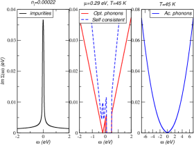
Figure 4: (color online) Electronic self-energy due to unitary scatterers and acoustic and optical phonons. Only the imaginary part is represented. The impurity concentration is $n_{i}=0.0002$. The self-energy due to optical phonons depends on temperature and on the chemical potential $\mu$. We have chosen $\mu=0.29$ eV and $T=45$ K. In the central panel we show the calculation for self-energy due to optical phonons both using the bare electronic Green’s function (solid line) and the Green’s function with mid-gap states (dashed line). The acoustic self-energy is independent of the chemical potential and is represented for a temperature of $T=45$ K.

In Fig. 4, we depicted the self energy of the short ranged impurities together with those due to acoustic and optical phonons. It clear that the effect of acoustic phonons is negligible at low energies. The self-energy due to optical phonons depends on the chemical potential, and is represented for a gate voltage of $V_{g}=71$ V ($\mu=0.29$ eV).

III.3.2 Effect of Disorder: Phononic Propagator

To be consistent, also the phonon propagator has to be dressed due to its interaction with impurities. The phonon propagator shall be renormalized within the RPA-approximation, i.e.,

$$D_{\nu}^{RPA}(i\omega_{n})=\frac{2\omega_{\nu}}{(i\omega_{n})^{2}-(\omega_{\nu})^{2}-2\omega_{\nu}\Pi_{\nu}(i\omega_{n})}$$ (65)

where the first order of the phononic self-energy $\Pi_{\nu}(\omega_{n})$ is proportional to the polarization defined as

$$P^{(1)}(\omega_{n})=\lim_{\vec{q}\rightarrow 0}\frac{1}{A_{s}}\int_{0}^{\hbar\beta}d\tau e^{i\omega_{n}\tau}\langle T_{\tau}\rho(\vec{q},\tau)\rho(-\vec{q},0)\rangle\;,$$ (66)

with $\rho(-\vec{q})$ denoting the density operator. Explicitly, we get for the imaginary part of the retarded phononic self-energy

$$\Im\Pi_{\nu}^{ret}(\omega) =\frac{\hbar}{M\omega_{\nu}}\left(\frac{\partial t}{\partial a}\right)^{2}\frac{18}{\sqrt{3}\pi t^{2}}\int\frac{d\omega_{1}}{2\pi}\Theta(\omega_{1},\omega)$$

$$\times\left[n_{F}(\omega_{1}\hbar-\mu)-n_{F}(\omega_{1}\hbar+\omega\hbar-\mu)\right]\;,$$ (67)

where the dimensional function $\Theta(\omega_{1},\omega)$ is given in Appendix B.

In Fig. 5, the self-energy due to electron-phonon scattering (left) and the conductivity (right) are shown as they result using the bare (dashed) and dressed (full) phonon propagator. Since the effect is hardly appreciable, we show also the results where the phononic self-energy has been multiplied by a factor 10 (dotted-dashed). The renormalization of the phonon propagator due to disorder is thus negligible and the results of the following section will be obtained using the bare phonon propagator.

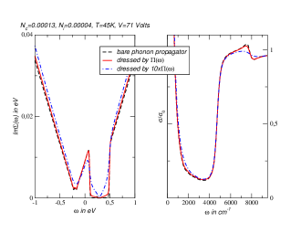
Figure 5: (color online) Electronic self-energy due to electron-optical phonon interaction $\Im\Sigma_{opt}^{ret}$ (left) and optical conductivity $\sigma$ (right) for various phonon propagators. The electronic propagator is dressed by the self-energies due to Coulomb ($n_{C}=0.00013$) and impurity scattering ($n_{i}=0.00004$). The temperature is $T=45$K and the applied gate voltage $V=71$Volts.

IV The DC and AC conductivity

In this section, we discuss the transport properties of graphene due to the various sources of one-particle scattering. This is done within the Kubo formalism.

IV.1 The Kubo formula

The Kubo formula for the conductivity is given by

$$\sigma_{xx}(\omega)=\frac{<j^{D}_{x}>}{iA_{s}(\omega+i0^{+})}+\frac{\Lambda_{xx}(\omega+i0^{+})}{i\hbar A_{s}(\omega+i0^{+})}\,,$$ (68)

with $A_{s}=N_{c}A_{c}$ the area of the sample, and $A_{c}=3\sqrt{3}a^{2}/2$ the area of the unit cell, from which it follows that

$$\Re\sigma_{xx}(\omega)=D\delta(\omega)+\frac{\Im\Lambda_{xx}(\omega+i0^{+})}{\hbar\omega A_{s}}\,,$$ (69)

and

$$\Im\sigma_{xx}(\omega)=-\frac{<j^{D}_{x}>}{A_{s}\omega}-\frac{\Re\Lambda_{xx}(\omega+i0^{+})}{\hbar\omega A_{s}}\,,$$ (70)

where $D$ is the charge stiffness which reads

$$D=-\pi\frac{<j^{D}_{x}>}{A_{s}}-\pi\frac{\Re\Lambda_{xx}(\omega+i0^{+})}{\hbar A_{s}}\,.$$ (71)

The function $\Lambda_{xx}(\omega+i0^{+})$ is obtained from the Matsubara current-current correlation function, defined as

$$\Lambda_{xx}(i\omega_{n})=\int_{0}^{\beta}d\,\tau e^{i\omega_{n}\tau}<T_{\tau}j^{P}_{x}(\tau)j^{P}_{x}(0)>\,.$$ (72)

The calculation of the conductivity amounts to the determination of the current-current correlation function.

IV.2 The real part of the DC conductivity

The real part of the DC conductivity is given by

$$\Re\sigma(\mu)=-\frac{2e^{2}}{\pi h}\int{d\epsilon}K(\epsilon)\frac{\partial f(\epsilon-\mu)}{\partial\epsilon}\,,$$ (73)

where $f(x)$ is the Fermi function and $K(\epsilon)$ is a dimensionless function that depends on the full self-energy. In the limit of zero temperature the derivative of the Fermi function tends to a delta-function and the conductivity is given by

$$\Re\sigma(\mu)=\frac{2e^{2}}{\pi h}K(\mu)\,,$$ (74)

with $K(\mu)$ given by

$$K(\mu) = \frac{1}{2I_{a}}\sum_{s=\pm 1}\Big{(}\frac{D(sA+D)I_{a}}{(A+sD)^{2}+I_{a}^{2}}+A\arctan\frac{A}{I_{a}}-A\arctan\frac{A+sD}{I_{a}}\Big{)}$$

$$+ \frac{I_{a}}{2A}\Big{(}2\arctan\frac{A}{I_{a}}-\arctan{A-D}{I_{a}}-\arctan\frac{A+D}{I_{a}}\Big{)}\,,$$

and

$$I_{a}=\hbar\Im\Sigma(\mu)\,,\,A=\mu-\hbar\Re\Sigma(\mu)\,$$ (75)

and $D$ the cutoff bandwidth.

In Fig. 6 we plot $\sigma_{DC}(\mu)$ as function of the gate voltage, $V_{g}$, considering the effects of both charged impurities, mid-gap states and acoustic phonons (the optical phonons do not contribute to $\sigma_{DC}(\mu)$). It is clear that the linear behavior of $\sigma_{DC}(\mu)$ as function of $V_{g}$ is recovered. The theoretical curves are plotted together with the experimental data of Ref. [Basov, ]. After having fitted the experimental curves, it is clear that the most dominant contribution to the DC conductivity is coming from Coulomb impurities.

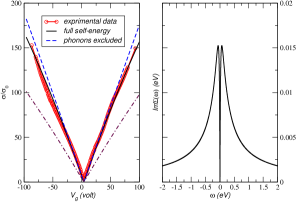
Figure 6: (color online) Left panel: Experimental data (circles) from Ref. [Basov, ], conductivity with the full self-energy (solid line) due to phonons, mid-gap states, and charged impurities, conductivity (dashed-line) with self-energy due to mid-gap states and charged impurities, only. The parameters are $T=45$ K, $n_{i}=4\times 10^{-5}$, $n_{i}^{C}=7.5\times 10^{-5}$, and $d=0$. The dashed-dotted line is the same as the solid line but with $n_{i}^{C}=1.3\times 10^{-4}$. Right panel: Imaginary part of the self-energy, $\hbar\Im\Sigma_{Coul}^{ret}(\bm{K},\omega)$, due to charged impurities, the most dominant contribution.

Let us now further discuss the conductivity as function of the gate voltage $V_{g}$, which relates to the chemical potential as $V_{g}\propto\mu^{2}$. In Figure 7 we show $\sigma(\mu)$ as function of $V_{g}$ considering both charged impurities and short range scatterers (left panel), having the same impurity concentration. We note that the conductivity, albeit mostly controlled by charged impurities still has finger prints of the finite $\epsilon_{0}$ scatterers, due to the asymmetry between the hole (negative $V_{g}$) and particle (positive $V_{g}$) branches. The conductivity follows closely the relation $\sigma(\mu)\propto V_{g}$, except close to the Dirac point where is value its controlled by the short range scattering.

If we suppress the scattering due to charged impurities, which should be the case in suspended graphene, only the scattering due to short range scatterers survive. In this case the right panel of Fig. 7 shows that there is a strong asymmetry between the hole and the particle branches of the conductivity curve even for a value of $\epsilon_{0}$ as large as 100 eV. Moreover, the smaller the value of $\epsilon_{0}$ the larger is the asymmetry in the conductivity curve. We note that asymmetric conductivity curves were recently observed. Andrei On the contrary, if the experimental data shows particle-hole symmetry of $\sigma(\mu)$ around the Dirac point, then the dominant source of scattering is coming from very strong short range potentials, i.e., scatterers that are in the unitary limit.

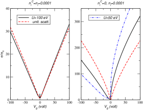
Figure 7: (color online) Left: Conductivity $\sigma(\mu)$, in units of $\sigma_{0}=\pi e^{2}/(2h)$, considering both short range and charged scatterers. Righ: Conductivity $\sigma(\mu)$ when the influence of charge scatterers is removed.

IV.3 The real part of the AC conductivity

The finite frequency part of the conductivity is given by

$$\Re\sigma(\omega)=\frac{2e^{2}}{\pi h}\int\frac{d\omega_{1}}{\omega}\Theta(\omega_{1},\omega)[f(\hbar\omega_{1}-\mu)-f(\hbar\omega_{1}+\hbar\omega-\mu)]\,,$$ (76)

where $f(x)$ is the Fermi function and $\Theta(\omega_{1},\omega)$ is a dimensionless function given in Appendix B. As can be see from this Appendix, the function $\Theta(\omega_{1},\omega)$ depends on the self energy, which is due both to impurities and phonons.

IV.3.1 Optical conductivity without Coulomb scatterers

We will first discuss the optical conductivity without Coulomb scatterers since they should not be present in suspended graphene. In Figure 8, we plot the conductivity of a graphene plane in units of $\sigma_{0}=\frac{\pi}{2}e^{2}/h$. The calculation is made at two different temperatures, $T=45$ K and $T=300$ K, and for a density of impurities $n_{i}=0.0004$. The calculation compares the conductivity with and without the effect of the phonons. The main effect induced by short-ranged impurities is the existence of a finite light-absorption in the frequency range $0<\hbar\omega<2\mu$. The optical phonons increase the absorption in this frequency range. We have checked that the effect of the acoustic phonons is negligible. The optical phonons also induce a conductivity larger than $\sigma_{0}$ for frequencies above $\omega=2\mu$. The effect is more pronounced at low temperatures.

Figure 8: (color online) Optical conductivity of graphene at two different temperatures $T=$45, 300 K. Each panel has two curves, the solid curve is the conductivity with only short-ranged impurities, the dashed curve is the conductivity with both short-ranged impurities and phonons, with the self-energy due to phonons computed with the full Green’s function. The chemical potential is that associated with a gate voltage of $V_{g}=71$ V. The vertical, dashed line marks twice this value.

In Figure 9, we again plot the conductivity of a graphene plane in units of $\sigma_{0}=\frac{\pi}{2}e^{2}/h$ and at temperature $T=45$ K. This time we compare different impurity densities $n_{i}$ (left hand side) and gate voltages/chemical potentials (right hand side). There is more absorption for frequencies in the region $0<\hbar\omega<2\mu$ the larger the impurity concentration is. This is because the number of mid-gap states is proportional to $\sqrt{n}_{i}$.PeresPRB For larger gate-voltage a plateau is reached at frequencies in $0<\hbar\omega<2\mu$. For small gate voltages, $V_{g}$, the absorption in the region $0<\hbar\omega<2\mu$ is larger than for larger $V_{g}$.

Figure 9: (color online) Optical conductivity of graphene at temperature $T=$45 K. The left hand side shows curves for various short-ranged impurity densities $n_{i}$. The right hand side shows curves for various gate voltage $V_{g}$. The vertical, dashed lines mark twice the chemical potential.

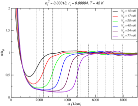
Figure 10: (color online) Real part of the optical conductivity including the effect of phonons, midgap states and charged impurities. The parameters are $T=45$ K, $n_{i}=4.0\times 10^{-5}$, and $n_{i}^{C}=1.3\times 10^{-4}$. The dashed vertical lines correspond to $\hbar\omega=2\mu$ and the shorter dotted-dashed ones to $\hbar\omega=2\hbar\omega_{0}+2\mu$.

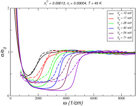
Figure 11: (color online) Real part of the optical conductivity including the effect of phonons, mid-gap states and charged impurities, compared with the experimental data from Ref. [Basov, ]. The parameters are $T=45$ K, $n_{i}=4.0\times 10^{-5}$, $n_{i}^{C}=1.3\times 10^{-4}$, and $d=0$.

IV.3.2 Optical conductivity with Coulomb scatterers

We will now discuss the optical conductivity with Coulomb scatterers which are generally present in graphene on a substrate Chen . In Figure 10, we plot the conductivity of a graphene plane in units of $\sigma_{0}=\frac{\pi}{2}e^{2}/h$, including the effect of midgap states, charged impurities and phonons. Again, the main feature is that the conductivity is finite in the range $0<\hbar\omega<2\mu$ and increases as the gate voltage decreases. We choose the concentration of midgap states in Fig. 10 to be one order of magnitude smaller than the one of Coulomb scatterersStauberBZ , and therefore the conductivity is mainly controlled by phonons and charged impurities.

Another feature of the curves in Fig. 10 is the large broadening of the interband transition edge at $\hbar\omega=2\mu$ (indicated by vertical dashed lines). Note that this broadening is not due to temperature but to charged impurities, instead. In fact, the broadening for all values of $V_{g}$ is larger when the conductivity is controlled by charged impurities rather than by midgap states.

The coupling to phonons produces a feature centered at $2\hbar\omega_{0}+2\mu$ where $\hbar\omega_{0}$ denotes the LO-phonon energy corresponding to the wave number 1600cm^-1 (indicated by shorter dotted-dashed vertical lines). For gate voltages with $\mu<\hbar\omega_{0}$ there appears a similar feature at $2\hbar\omega_{0}-2\mu$ which is not washed out by disorder. The optical phonons thus induce a conductivity larger than $\sigma_{0}$ around these frequencies. This effect is washed out at larger temperatures and $\sigma<\sigma_{0}$.

All these effects are consistent with the recent infrared measurements of graphene on a SiO₂ substrate Basov which are shown as dashed lines in Fig. 11. Notice that there is only one fitting parameter involved which is adjusted by the conductivity curve at zero chemical potential. Whereas for low gate voltage the agreement is good, there is considerable weight missing for higher gate voltage ($V>20$ Volts). Nevertheless, all theoretical lines predict lower conductivity than the experimental measurements, such that our model with only one fitting parameter is consistent. Since we have included in our calculation all possible one-particle scattering mechanisms, the missing weight at large gate voltages could be attributed to electron-electron interactions in graphene, which become important at this electronic densities.

V Discussion and conclusions

In this paper we have computed the optical conductivity of graphene at finite chemical potential, generalizing the results of Ref. [PeresPRB, ]. The calculation includes both the effect of disorder (mid-gap states and charged impurities, which have a different signature in the DC conductivitySchliemann ) and the effect of phonons (optical and acoustic). It is shown that at low temperatures the effect of acoustic phonons in negligible, since it induces an imaginary part of the electrons’ self-energy that is much smaller than the imaginary part induced by the impurities. For a discussion based on the Boltzmann equation, see Ref. StauberBZ, .

The imaginary part induced by optical phonons is of the order of the imaginary part induced by impurities. Still, optical phonons are only important in the calculation of the real part of $\sigma(\omega)$, they play no role in the calculation of $\sigma_{DC}(\mu)$ in the temperature range $T\in[0,300]$ K. The self-energies due to mid-gap states and due to optical phonons are in a sense complementary, since the imaginary part coming from impurities is large at the Dirac point, whereas the imaginary part coming from the optical phonons increase linearly with the energy away from the Dirac point. The imaginary part of the self energy due to charged impurities is a non-monotonous function of the energy, growing first linearly but changing to a decaying behavior of the form $1/\omega$, for large energies.

In Section IV, we have discussed the different scattering mechanisms separately, since for suspended graphene Coulomb scatterers will be absent. Since vacancies, corresponding to an infinite potential where particle-hole symmetry is restored, are unlikely, we model the short-ranged potentials due to cracks, ripples, etc. by large, but finite short ranged potential. For the DC conductivity, this leads to an asymmetry of the hole- and electron-doped regime.

The most notable effect on the optical conductivity of both the optical phonons and the impurities is the induction of a finite energy absorption in the energy range $0<\hbar\omega<2\mu$, a region where the clean theory predicts a negligible absorption. The optical phonons also induce a conductivity larger than $\sigma_{0}$ around $\hbar\omega\simeq 2\mu$. It is interesting to note that for frequencies away from the Dirac point the imaginary part of the self-energy due to optical phonons is linear in frequency, a behavior similar to that due to electron-electron interactions in graphene.

It is clear from Fig. 11 that in general the calculated absorption in the range $0<\hbar\omega<2\mu$ is not as large as the experimental one. It is also noticeable that for small gate voltages there is a reasonable fit of both the absorption and of the broadening of the of the step around $2\mu$. For large values of the gate voltage the calculated absorption is smaller than the measured one. This suggests that some additional scattering mechanism is missing in the calculation of the optical conductivity. The missing mechanism has to be more effective at large gate voltage. A possibility are plasmons of the type found in Ref. [Mikhailov, ]. Another possibility is that water molecules which are especially active in the infrared regime, are contributing to the missing weight.

In synthesis we have provided a complete and self-consistent description of the optical conductivity of graphene on a substrate (including Coulomb scatterers) and suspended (without Coulomb scatterers). Our results are in qualitative agreement with the experimental results. To meet a quantitative agreement further research (also on suspended graphene) is necessary, but water molecules underneath the graphene sheet are likely to account for the missing weight.

Appendix A An approximate phonon model

We start by expanding the matrix elements of the dynamical matrix (10) up to second order in the momentum $\bm{Q}$. We then introduce acoustic, $\bm{u}=(\bm{u}_{A}+\bm{u}_{B})/\sqrt{2}$, and optical, $\bm{v}=(\bm{u}_{A}-\bm{u}_{B})/\sqrt{2}$, modes. This procedure leads to the following eigenvalue problem

$$M_{C}\omega^{2}\left(\begin{array}[]{c}\bm{u}\\ \bm{v}\end{array}\right)=\left(\begin{array}[]{cc}B_{1}&B_{2}\\ B_{2}^{\dagger}&B_{3}\end{array}\right)\left(\begin{array}[]{c}\bm{u}\\ \bm{v}\end{array}\right)\,,$$ (77)

with

$$B_{1}=\frac{3a^{2}}{32}\left(\begin{array}[]{cc}y_{1}&4\alpha Q_{x}Q_{y}\\ 4\alpha Q_{x}Q_{y}&y_{2}\end{array}\right)\,,$$ (78)

with $y_{1}=3(2\alpha+3\beta)Q_{x}^{2}+(2\alpha+9\beta)Q_{y}^{2}$ and $y_{2}=(2\alpha+9\beta)Q^{2}_{x}+3(2\alpha+3\beta)Q^{2}_{y}$. Further, we have

$$B_{2}=\frac{3ia^{2}}{8}(2\alpha-9\beta)\left(\begin{array}[]{cc}Q_{x}&Q_{y}\\ Q_{y}&Q_{x}\end{array}\right)\,,$$ (79)

and

$$B_{3}=\frac{3a^{2}}{32}\left(\begin{array}[]{cc}y_{3}&(36\beta-4\alpha)Q_{x}Q_{y}\\ (36\beta-4\alpha)Q_{x}Q_{y}&y_{4}\end{array}\right)\,,$$ (80)

with $y_{3}=32\alpha+144\beta-(6\alpha+9\beta)Q^{2}_{x}-(2\alpha+45\beta)Q_{y}^{2}$ and $y_{3}=32\alpha+144\beta-(6\alpha+9\beta)Q^{2}_{y}-(2\alpha+45\beta)Q_{x}^{2}$ . The eigenvalue problem can be put in the form

$$B_{1}\bm{u}+B_{2}\bm{v}=M_{C}\omega^{2}\bm{u}$$ (81)

$$B_{2}^{\dagger}\bm{u}+B_{3}\bm{v}=M_{C}\omega^{2}\bm{v}$$ (82)

Let us first look at the acoustic modes. They corresponds to $\omega\simeq 0$. In this case we can write

$$\bm{v}\simeq-\frac{B_{2}^{\dagger}}{3(\alpha+9\beta/2)}\bm{u}\,,$$ (83)

from which an eigenvalue equation for $\bm{u}$ follows:

$$B_{1}\bm{u}-\frac{B_{2}B_{2}^{\dagger}}{3(\alpha+9\beta/2)}\bm{u}=M\omega^{2}\bm{u}\,.$$ (84)

In the case of the optical modes one has $M\omega^{2}\simeq 3\alpha+27\beta/2$, from which we can write

$$\bm{u}\simeq\frac{B_{2}}{3(\alpha+9\beta/2)}\bm{v}\,,$$ (85)

which leads to

$$B_{3}\bm{v}+\frac{B_{2}^{\dagger}B_{2}}{3(\alpha+9\beta/2)}\bm{v}=M\omega^{2}\bm{v}\,.$$ (86)

The dashed-dotted lines in Fig. 1 are the eigenvalues of Eqs. (84) and (86).

Appendix B The function $\Theta(\omega_{1},\omega)$

In Eq. (76) the dimensionless $\Theta(\omega_{1},\omega)$ function was introduced. Let us define

$$A = \hbar\omega_{1}-\hbar\Sigma^{\prime}(\omega_{1})\,,$$ (87)

$$B = \hbar\omega_{1}+\hbar\omega-\hbar\Sigma^{\prime}(\omega_{1}+\omega)\,,$$ (88)

$$I_{a} = \hbar\Sigma^{\prime\prime}(\omega_{1})\,,$$ (89)

$$I_{b} = \hbar\Sigma^{\prime\prime}(\omega_{1}+\omega)\,,$$ (90)

$$D_{1} = 2[(A-B)^{2}+(I_{a}-I_{b})^{2}]\times$$ (91)

$$[(A-B)^{2}+(I_{a}+I_{b})^{2}]\,,$$

$$D_{2} = 2[(A+B)^{2}+(I_{a}-I_{b})^{2}]\times$$ (92)

$$[(A+B)^{2}+(I_{a}+I_{b})^{2}]\,.$$

The function $\Theta(\omega_{1},\omega)$ is expressed in terms of the above auxiliary functions as follows

$$\Theta(\omega_{1},\omega) = \frac{2}{D_{1}}I_{b}(A^{3}-2A^{2}B-2BI_{a}^{2}+A(B^{2}+I_{b}^{2}+I_{a}^{2}))\sum_{\alpha=\pm 1}\left(\arctan\frac{A}{I_{a}}-\arctan\frac{A+\alpha D}{I_{a}}\right)$$ (93)

$$+ \frac{2}{D_{1}}I_{a}(B^{3}-2B^{2}A-2AI_{b}^{2}+B(A^{2}+I_{a}^{2}+I_{b}^{2}))\sum_{\alpha=\pm 1}\left(\arctan\frac{A}{I_{b}}-\arctan\frac{A+\alpha D}{I_{b}}\right)$$

$$+ \frac{2}{D_{2}}I_{b}(A^{3}+2A^{2}B+2BI_{a}^{2}+A(B^{2}+I_{b}^{2}+I_{a}^{2}))\sum_{\alpha=\pm 1}\left(\arctan\frac{A}{I_{a}}-\arctan\frac{A+\alpha D}{I_{a}}\right)$$

$$+ \frac{2}{D_{2}}I_{a}(B^{3}+2B^{2}A+2AI_{b}^{2}+B(A^{2}+I_{a}^{2}+I_{b}^{2}))\sum_{\alpha=\pm 1}\left(\arctan\frac{A}{I_{b}}-\arctan\frac{A+\alpha D}{I_{b}}\right)$$

$$+ \left(\frac{1}{D_{1}}+\frac{1}{D_{2}}\right)I_{a}I_{b}(A^{2}-B^{2}+I^{2}_{a}-I^{2}_{b})\sum_{\alpha=\pm 1}\left(\log\frac{A^{2}+I_{a}^{2}}{B^{2}+I_{b}^{2}}-\log\frac{(A-\alpha D)^{2}+I_{a}^{2}}{(B-\alpha D)^{2}+I_{b}^{2}}\right)\,.$$

References

- (1) K. S. Novoselov, D. Jiang, T. Booth, V.V. Khotkevich, S. M. Morozov, A. K. Geim, Proc. Natl. Acad. Sci. USA 102, 10451 (2005).
- (2) K. S. Novoselov, A. K. Geim, S. V. Morozov, D. Jiang, M. I. Katsnelson, I. V. Grigorieva, S. V. Dubonos, and A. A. Firsov, Nature 438, 197 (2005).
- (3) Y. Zhang, Y.-W. Tan, H. L. Stormer, and P. Kim, Nature 438, 201 (2005).
- (4) K. S. Novoselov, A. K. Geim, S. V. Morozov, D. Jiang, Y. Zhang, S. V. Dubonos, I. V. Grigorieva, and A. A. Firsov, Science 306, 666 (2004).
- (5) A. K. Geim and K. S. Novoselov, Nature Materials 6, 183 (2007).
- (6) M. I. Katsnelson, Materials Today 10, 20 (2007).
- (7) A. H. Castro Neto, F. Guinea, and N. M. R. Peres, Phys. World 19, 33 (2006).
- (8) A. K. Geim and A. H. MacDonald, Physics Today 60, 35 (2007).
- (9) A. H. Castro Neto, F. Guinea, N. M. R. Peres, K. S. Novoselov, and A. K. Geim, Rev. Mod. Phys. [in press], arXiv:0709.1163.
- (10) C. W. Beenakker, arXiv:0710.3848.
- (11) P. C. Wallace, Phys. Rev. 71, 622 (1947).
- (12) G. W. Semenoff, Phys. Rev. Lett. 53, 2449 (1984).
- (13) F. D. M. Haldane, Phys. Rev. Lett. 61, 2015 (1988).
- (14) A. W. W. Ludwig, M. P. A. Fisher, R. Shankar, and G. Grinstein, Phys. Rev. B 50, 7526 (1994).
- (15) S. Ryu, C. Mudry, A. Furusaki, and A. W. W. Ludwig, Phys. Rev. B 75, 205344 (2007).
- (16) K. Ziegler, Phys. Rev. B 75, 233407 (2007).
- (17) V. P. Gusynin, S. G. Sharapov, and J. P. Carbotte, Int. Jour. of Mod. Phys. B 21, 4611 (2007).
- (18) E. V. Gorbar, V. P. Gusynin, V. A. Miransky, and I. A. Shovkovy, Phys. Rev. B 66, 045108 (2002).
- (19) L. A. Falkovsky and A. A. Varlamov, Eur. Phys. J. B 56, 281 (2007).
- (20) N. M. R. Peres, F. Guinea, and A. H. Castro Neto, Phys. Rev. B 73, 125411 (2006).
- (21) N. M. R. Peres and T. Stauber, Int. J. Mod. Phys. B 22, 2529 (2008).
- (22) M. I. Katsnelson, Eur. Phys. J. B 51, 157 (2006).
- (23) J. Tworzydlo, B. Trauzettel, M. Titov, A. Rycerz, and C. W. Beenakker, Phys. Rev. Lett. 96, 246802 (2006).
- (24) E. Louis, J. A. Verges, F. Guinea, and G. Chiappe, Phys. Rev. B 75, 085440 (2007).
- (25) F. Miao, S. Wijeratne, Y. Zhang, U. C. Coskun, W. Bao, and C. N. Lau, Science 317, 1530 (2007).
- (26) Z. Q. Li, E. A. Henriksen, Z. Jiang, Z. Hao, M. C. Martin, P. Kim, H. L. Stormer, and D. N. Basov, Nature Physics 4, 532 (2008).
- (27) Jahan M. Dawlaty, Shriram Shivaraman, Jared Strait, Paul George, Mvs Chandrashekhar, Farhan Rana, Michael G. Spencer, Dmitry Veksler, and Yunqing Chen, arXiv:0801.3302.
- (28) R. R. Nair, P. Blake, A. N. Grigorenko, K. S. Novoselov, T.J. Booth, T. Stauber, N. M. R. Peres, and A. K. Geim , Science 320, 1308 (2008).
- (29) A. B. Kuzmenko, E. van Heumen, F. Carbone, and D. van der Marel, Phys. Rev. Lett. 100, 117401 (2008).
- (30) K. Nomura and A. H. MacDonald, Phys. Rev. Lett. 96, 256602 (2006)
- (31) S. Adam, E. H. Hwang, V. M. Galitski, and S. Das Sarma, Proc. Natl. Acad. Sci. USA 104, 18392 (2007).
- (32) N. M. R. Peres, J. M. B. Lopes dos Santos, and T. Stauber, Phys. Rev. B 76, 073412 (2007).
- (33) T. Stauber, N. M. R. Peres, and F. Guinea, Phys. Rev. B 76, 205423 (2007).
- (34) Y.-W. Tan, Y. Zhang, K. Bolotin, Y. Zhao, S. Adam, E.H. Hwang, S. Das Sarma, H. L. Stormer, and P. Kim, Phys. Rev. Lett. 99, 246803 (2007).
- (35) V. V. Cheianov, V. I. Fal’ko, B. L. Altshuler, and I. L. Aleiner, Phys. Rev. Lett. 99, 176801 (2007).
- (36) T. Stauber, N. M. R. Peres, and A. K. Geim, Phys. Rev. B 78, 085432 (2008).
- (37) L. X. WangZhi and K. Mullen, Nano Lett. 8, 323 (2008).
- (38) P. Blake, P. D. Brimicombe, R. R. Nair, T. J. Booth, D. Jiang, F. Schedin, L. A. Ponomarenko, S. V. Morozov, H. F. Gleeson, E. W. Hill, A. K. Geim, and K. S. Novoselov, Nano Lett. 8, 1704 2008.
- (39) Junbo Wu, Héctor A. Becerril, Zhenan Bao, Zunfeng Liu, Yongsheng Chen, and Peter Peumans, Appl. Phys. Lett. 92, 263302 (2008).
- (40) V. P. Gusynin, S. G. Sharapov, Phys. Rev. B 73, 245411 (2006).
- (41) V. P. Gusynin, S. G. Sharapov, and J. P. Carbotte, Phys.Rev.Lett. 96, 256802 (2006).
- (42) V. P. Gusynin, S. G. Sharapov, and J. P. Carbotte, Phys.Rev.Lett. 98, 157402 (2007).
- (43) V. P. Gusynin, S. G. Sharapov, and J. P. Carbotte, Phys. Rev. B 75, 165407 (2007).
- (44) Thomas G. Pedersen, Phys. Rev. B 67, 113106 (2003).
- (45) Thomas G. Pedersen, Christian Flindt, Jesper Pedersen, Antti-Pekka Jauho, Niels Asger Mortensen, and Kjeld Pedersen, Phys. Rev. B 77, 245431 (2008).
- (46) T. Stauber and N. M. R. Peres, J. Phys.: Condens. Matter 20, 055002 (2008).
- (47) L. M. Woods and G. D. Mahan, Phys. Rev. B 61, 10651 (2000).
- (48) Hidekatsu Suzuura and Tsuneya Ando, Phys. Rev. B 65, 235412 (2002).
- (49) Tsuneya Ando, J. Phys. Soc. Jpn. 75, 124701 (2006)
- (50) Kohta Ishikawa and Tsuneya Ando, J. Phys. Soc. Jpn. 75, 84713 (2006).
- (51) A. H. Castro Neto and F. Guinea, Phys. Rev. B 75, 45404 (2007).
- (52) József Cserti and Géza Tichy, European J. of Phys. 25, 723 (2004).
- (53) There is some TEM evidence for the presence of vacancies in graphene, altouhg it is not clear at the presence if their origin is intrinsic or extrinsic, Dra. Ursel Bangert private communication.
- (54) Vitor M. Pereira, F. Guinea, J. M. B. Lopes dos Santos, N. M. R. Peres, and A. H. Castro Neto, Phys. Rev. Lett. 96, 036801 (2006).
- (55) Kentaro Nomura and A.H. MacDonald, Phys. Rev. Lett. 98, 076602 (2007).
- (56) J. H. Chen, C. Jang, M. S. Fuhrer, E. D. Williams, M. Ishigami, Nature Physics 4, 377 (2008).
- (57) Xu Du, I. Skachko, A. Barker, and E. Y. Andrei, Nat. Nanotechnol. 3, 491 (2008).
- (58) Maxim Trushin and John Schliemann, Europhys. Lett. 83, 17001 (2008).
- (59) S. A. Mikhailov and K. Ziegler, Phys. Rev. Lett. 99, 16803 (2007).