Magnetic breakdown of cyclotron orbits in systems with Rashba and Dresselhaus spin-orbit coupling

Abstract

We study the effect of the interplay between the Rashba and the Dresselhaus spin-orbit couplings on the transverse electron focusing in two-dimensional electron gases. Depending on their relative magnitude, the presence of both couplings can result in the splitting of the first focusing peak into two or three. This splitting has information about the relative value of spin-orbit couplings and therefore about the shape of the Fermi surface. More interesting, the presence of the third peak is directly related to the tunneling probability (”magnetic breakdown”) between orbits corresponding to the different sheets of the Fermi surface. In addition, destructive interference effects between paths that involve tunneling and those that do not can be observed in the second focusing condition. Such electron paths (orbits) could be experimentally detected using current techniques for imaging the electron flow opening the possibility to directly observe and characterize the magnetic breakdown effect in this system.

I Introduction

Transport properties of two-dimensional electron (2DEG) and hole gases can be affected in very peculiar ways by the spin-orbit (SO) coupling. The unusual properties of spin transport of these systems are seen as promising tools for the development of new spintronic devices,Awschalom et al. (2002) which would allow us to coherently control and manipulate the electrons’ spin. This triggered an intense activity in the field during the past years. Among the SO-related effects in 2DEGs, it is worth mentioning the proposal of a spin filtering transistor,Datta and Das (1990); Schliemann et al. (2003) the Aharonov-Casher oscillation in mesoscopic rings,König et al. (2006); Kovalev et al. (2007) and the spin Hall effect.Dyakonov and Perel (1971); Hirsch (1999); Murakami et al. (2003); Sinova et al. (2004); Kato et al. (2004); Usaj and Balseiro (2005); Wunderlich et al. (2005); Kato et al. (2005); Sih et al. (2005); Nikolic et al. (2005); Nomura et al. (2005a); Engel et al. (2005); Erlingsson and Loss (2005); Nomura et al. (2005b); Adagideli and Bauer (2005); Reynoso et al. (2006a)

In 2DEGs made either from heterostructures or from quantum wells, there are two dominating forms of the SO coupling.Winkler (2003) The Rashba SO coupling, which arises from the asymmetry of the confinement potential of the 2DEG, and the Dresselhaus SO coupling, which arises from the lack of inversion symmetry of the crystal structure. Both types of SO couplings are present in general and their relative magnitude depends on the structure and the materials used to make the 2DEG. The SO couplings are relatively weak in AlGaAs-GaAs structures and quite strong in In or Sb based semiconductors. There are two important differences between the Rashba and Dresselhaus SO couplings. On the one hand, the magnitude of the former can be externally controlled by a gate voltage,Nitta et al. (1997); König et al. (2006) providing a interesting new knob to control transport properties. On the other hand, the Rashba coupling is isotropic while the Dresselhaus coupling depends on the orientation of the crystal axes. These two different sources of the SO coupling can be experimentally determined using different techniques. Ganichev et al. (2004); Giglberger et al. (2007); Miller et al. (2003); Meier et al. (2007, 2008)

Both (linear) SO couplings lead to similar electronic and transport properties when one dominates. However, very interesting effects arise when the two couplings have a similar magnitude. In particular, when both couplings are equal the spin and the momentum decouple. This effect has been proposed as a way to built up a spin transistor in disordered systems. Schliemann et al. (2003) In addition, it was argued that in that case the system contains unusually long-lived spin excitations.Bernevig et al. (2006) Indications of the presence of this excitations have been observed very recently.Weber et al. (2007) Also, the magnetic field anisotropy of the spin relaxation length in long wires made from 2DEGs in AlGaAs has been attributed to the closed values of the two couplings.Frolov et al. (2008)

It is therefore interesting to look for new alternatives where the effect of the competition between the Rashba and Dresselhaus couplings on the transport properties can be measured directly. In this work, we analyze the effect of such competition on the transverse electron focusing signal.van Houten et al. (1989); Beenakker and van Houten (1991) In Ref. [Usaj and Balseiro, 2004] it was predicted that SO coupling leads to the splitting of the odd focusing peaks. Since then, this splitting has been observed in different samples Rokhinson et al. (2004); Dedigama et al. (2006) and discussed by several authors. Reynoso et al. (2004); Zülicke et al. (2007); Schliemann (2008) Here, we show that the splitting of the focusing peaks can be used to map out the non-trivial shape of the Fermi surface of the 2DEGs when both types of linear SO couplings are present and have a similar magnitude. In addition, we found that the focusing experiment can clearly show the tunneling between cyclotron orbits, in direct analogy to the magnetic breakdown in bulk materials.Cohen and Falicov (1961); de Andrada e Silva et al. (1994)

To our knowledge, this is the first example where the magnetic breakdown between different cyclotron orbits could be directly observed. This could be done by using, for instance, the imaging technique developed by Westervelt and coworkers.Topinka et al. (2000, 2001); Aidala et al. (2006); Reynoso et al. (2006b); Aidala et al. (2007)

II Spin-orbit coupling in two dimensional gases

II.1 Bulk eigenstates

The Hamiltonian of a 2DEG in the presence of both Rashba and Dresselhaus SO couplings is given by

$$H=\frac{p^{2}}{2m^{*}}+\frac{\alpha}{\hbar}(p_{y}\sigma_{x}-p_{x}\sigma_{y})+\frac{\beta}{\hbar}(p_{x^{\prime}}\sigma_{x^{\prime}}-p_{y^{\prime}}\sigma_{y^{\prime}})$$ (1)

where $\bm{p}=(p_{x},p_{y})$ is the momentum operator, $\alpha$ and $\beta$ are the Rashba and Dresselhaus coupling parameters, respectively, and $\{\sigma_{i}\}$ are the Pauli matrices. The axes $x^{\prime}$ and $y^{\prime}$ correspond to crystallographic directions while $x$ and $y$ are arbitrary directions chosen in a convenient way—note that the Rashba term is isotropic and therefore independent of the axes choice.

Hamiltonian (1) can be easily diagonalized by proposing a solution in the form of a plane wave. The eigenfunctions and eigenvalues are

$$\Psi_{\bm{k}}^{\pm}(\bm{r}) = \frac{1}{\sqrt{2A}}\mathrm{e}^{\mathrm{i}\bm{k}\cdot\bm{r}}\left({{\pm 1\atop{\rm e}^{{\mathrm{i}}\phi}}}\right)$$ (2)

$$\varepsilon(\bm{k}) = \frac{\hbar^{2}k^{2}}{2m^{*}}\!\pm\!\sqrt{(\alpha k_{x}\!+\!\beta k_{y})^{2}\!+\!(\alpha k_{y}\!+\!\beta k_{x})^{2}}\,.$$ (3)

Here, $\tan\phi=-(\alpha k_{x}+\beta k_{y})/(\alpha k_{y}+\beta k_{x})$, $A$ is the system’s area and we choose $x=x^{\prime}$ and $y=y^{\prime}$. Figure 1 shows the corresponding Fermi surface for different values of the ratio $\beta/\alpha$. The arrows indicate the spin orientations of the eigenstates.

The competition between the Rashba and Dresselhaus SOs originates a deviation of the Fermi surface from the circular shape. For $\alpha=\pm\beta$ the Fermi surfaces recover a circular shape shifted from the $\Gamma$ point (there is a perfect nesting between the two surfaces) and the spin orientation becomes independent of $\bm{k}$—nevertheless, this case has interesting spin properties.Schliemann and Loss (2003); Mishchenko and Halperin (2003); Schliemann et al. (2003); Bernevig et al. (2006)

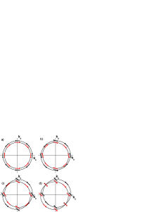
Figure 1: The Fermi surfaces for $\beta/\alpha\!=\!0,0.5,0.75$ and $1$ are shown in (a), (b), (c) and (d), respectively. The arrows indicate the spin orientation of the corresponding eigenstate.

For $|\beta/\alpha|\!\neq\!1$ the two different Fermi surfaces do not cross each other. The minimum and maximum distances between them in $k$-space are given by $\Delta k_{\pm}=\frac{2m^{*}}{\hbar^{2}}|\alpha\pm\beta|$. As we will show, these properties have important consequences on the transverse focusing signal .

When an external magnetic field is applied perpendicular to the sample, Landau levels are formed. In that case, a Zeeman term must be included in Hamiltonian (1) and $\bm{p}$ should be replaced by $\bm{p}+(e/c)\bm{A}$, with $\bm{A}$ as the vector potential. A closed analytical solution for arbitrary values of $\alpha$ and $\beta$ is not known (see however Refs. [Zarea and Ulloa, 2005; Zhang, 2006]). For $\beta=0$, however, a straightforward calculationBychkov and Rashba (1984) shows that the energy spectrum is given by $E_{n}^{\pm}\!=\!\hbar\omega_{c}n\mp(E_{0}^{2}+(\alpha/l_{c})^{2}2n)^{\frac{1}{2}}$, where $n\geq 1$, $\omega_{c}\!=\!e\left|B\right|/m^{*}c$ is the cyclotron frequency, $l_{c}\!=\!(\hbar/m\omega_{c})^{\frac{1}{2}}$ is the magnetic length, and $E_{0}\!=\!\hbar\omega_{c}/2-g\mu_{B}B_{z}/2$ is the energy of the ground state ($n\!=\!0$). In the limit of strong Rashba coupling or large $n$, $(\alpha/l_{c})\sqrt{2n}\gg E_{0}$, the spin of the eigenstates lies in the plane of the 2DEG. These eigenstates have a cyclotron radius given by

$$r_{c}^{2}\simeq 2nl_{c}^{2}.$$ (4)

Then, states with different $n$, and consequently different cyclotron radii, coexist within the same energy window.Usaj and Balseiro (2004) In fact, it is easy to verify that the difference between the two cyclotron orbits is

$$\Delta r_{c}\simeq\frac{2\alpha}{\hbar\omega_{c}}\!=\!\frac{\hbar\Delta k_{\pm}}{m^{*}\omega_{c}}\!=\!l_{c}^{2}\Delta k_{\pm}$$ (5)

Equivalent results are found in a semiclassical treatment of the problem.Pletyukhov et al. (2002); Reynoso et al. (2004); Rokhinson et al. (2004); Zülicke et al. (2007)

Eventually, if both $\alpha$ and $\beta$ were non-zero, one might hope to be able to gather information on the shape of the Fermi surface by measuring $\Delta r_{c}$. As we show below, this is indeed the case when transverse electron focusing is used to map out $\Delta r_{c}$ as a function of crystal orientation or the strength of the Rashba coupling.

II.2 Transverse electron focusing

The usual geometry for transverse focusing experiments consists of two quantum point contacts (QPCs) at a distance $L$, which are coupled to the same edge of a 2DEG (see Fig. 2). Electrons emitted from QPC $I$ (injector) are focalized onto the QPC $D$ (detector) by the action of an external magnetic field perpendicular to the 2DEG. In a classical picture, the electrons ejected from the injector are forced to follow circular orbits due to the Lorentz force. If the applied magnetic field has some arbitrary value, the electrons miss the detector and simply follow skipping orbits against the edge of the sample. However, for some particular values of the external field ($B_{n}$), such that the distance between the QPCs is $n$ times the diameter of the cyclotron orbit, with $n$ as an integer number, the electrons reach the detector. In such a case, there is a charge accumulation in the detector that generates a voltage difference across QPC $D$. This gives voltage peaks as the external field is swept through the focusing fields $B_{n}$.Tsoi (1975); van Houten et al. (1989); Potok et al. (2002)

In a quantum-mechanical description, the scattering states in the two QPC are coupled by the Landau levels of the 2DEG. As the Landau eigenstates have a characteristic length (the cyclotron radius $r_{c}$) that depends on the applied field, there is also a matching condition for $B=B_{n}$. In this context, the main features of the magnetic-field dependence of the measured signal are contained in the transmission $T$ between the two QPCBeenakker and van Houten (1991)—typical experimental setups include also one or two Ohmic contacts at the bulk of the 2DEG which are used to inject currents and measure voltages.van Houten et al. (1989)

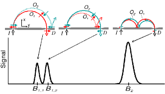
Figure 2: Scheme of the focusing experiment in the presence of SO coupling (we take $\beta=0$ for simplicity). An electron injected at QPC $I$ can follow one of two different orbits ($O_{1}$ and $O_{2}$) depending on its spin orientations. These two orbits lead to the splitting of the first focusing peak since the corresponding focusing fields $B_{1,1}$ and $B_{1,2}$ are different. After bouncing off the edge the electron that followed orbit the smaller (bigger) orbit continues in the bigger one (smaller one) so in both cases the electron arrives to the detector $D$ for the same focusing field $B_{2}$, leading to a single peak.

As shown in Refs. [Usaj and Balseiro, 2004] and [Rokhinson et al., 2004], in systems with either Rashba or Dresselhaus spin-orbit coupling (but not both) the first focusing peak splits in two. Such splitting, for $\beta=0$, is given by Eq. (5) or, in terms of the magnetic field, by $\Delta B\!=\!4\alpha m^{*}c/\hbar eL$, which is independent of $B$. Furthermore, each peak corresponds to a different spin projection of the electron leaving the emitter.Usaj and Balseiro (2004) Once again this can be understood using a classical picture plus the fact that there are two Fermi surfaces, even though the semiclassics is not trivial.Littlejohn and Flynn (1992); Frisk and Guhr (1993); Amann and Brack (2002); Pletyukhov et al. (2002); Zaitsev (2002); Pletyukhov and Zaitsev (2003); Zülicke et al. (2007)

This simple mechanism, which is able to spatially separate the two spin orientations of a electron beam, was recently usedRokhinson et al. (2006) to study the current’s spin polarization associated with the ”$0.7$” anomaly in QPCs and it was also suggestedReynoso et al. (2007) as a tool to study spin polarization of the flowing current in adiabatic QPCs due to SO.Eto et al. (2005)

II.3 Numerical solution

As mentioned above, we are interested in calculating the conductance between the two lateral QPCs. In the zero temperature limit this conductance is just $e^{2}/h$ times the transmission coefficient $T$ between the two contacts evaluated at the Fermi energy. Even in the absence of the spin-orbit interaction, it is not possible to obtain an analytical solution of the problem when there is an applied perpendicular magnetic field. Hence, we calculate $T(E_{F})$ numerically using a discretized system (”tight-binding-like” model) where the leads or contacts can be easily attached. The Hamiltonian of the system can then be written as $H=H_{0}+H_{SO}$, where

$$H_{0}\!=\!\sum_{n,\sigma}\varepsilon_{\sigma}c_{n\sigma}^{\dagger}c_{n\sigma}\!-\!\sum_{\langle n,m\rangle,\sigma}t_{nm}\,c_{n\sigma}^{\dagger}c_{m\sigma}\!+\!h.c.\,.$$ (6)

Here, $c_{n\sigma}^{\dagger}$ creates an electron at site $n$ with spin $\sigma$ ($\uparrow$ or $\downarrow$ in the $z$ direction) and energy $\varepsilon_{\sigma}\!=\!4t\!-\!\sigma g\mu_{B}B_{z}/2$, $t\!=\!$ $\hbar^{2}/2m^{*}a_{0}^{2}$, and $a_{0}$ is the effective lattice parameter which is always chosen to be small compared to the Fermi wavelength. The summation is made on a square lattice, where the position of the site $n$ is $n_{x}\widehat{\bm{x}}+n_{y}\widehat{\bm{y}}$, where $\widehat{\bm{x}}$ and $\widehat{\bm{y}}$ are unit vectors in the $x$ and $y$ directions, respectively. The hopping matrix element $t_{nm}$ is nonzero only for nearest-neighbor sites and includes the effect of the diamagnetic coupling through the Peierls substitution.Ferry and Goodnick (1997) For the choice of the Landau gauge $t_{n(n+\widehat{\bm{x}})}\!=\!t\exp{(-\mathrm{i}n_{y}2\pi\phi/\phi_{0})}$ and $t_{n(n+\widehat{\bm{y}})}\!=\!t$ with $\phi\!=\!a_{0}^{2}B$ the magnetic flux per plaquete and $\phi_{0}\!=\!hc/e$ the flux quantum.

The second term of the Hamiltonian describes the spin-orbit coupling,

$$H_{SO}\!=\!\sum_{n}\left\{\lambda_{y}c_{n\uparrow}^{\dagger}c_{(n+\widehat{\bm{y}})\downarrow}-\lambda_{y}^{*}c_{n\downarrow}^{\dagger}c_{(n+\widehat{\bm{y}})\uparrow}+\right.$$ (7)

$$\left.e^{-\mathrm{i}n_{y}2\pi\phi/\phi_{0}}\left[\lambda_{x}c_{n\uparrow}^{\dagger}c_{(n+\widehat{\bm{x}})\downarrow}\!-\!\lambda_{x}^{*}c_{n\downarrow}^{\dagger}c_{(n+\widehat{\bm{x}})\uparrow}\right]\right\}\!+\!h.c.$$

where $\lambda_{R}\!=\!\alpha/2a_{0}$, $\lambda_{D}\!=\!\beta/2a_{0}$, $\lambda_{x}\!=\!\left(\lambda_{R}\!+\!\mathrm{i}\lambda_{D}e^{-\mathrm{i}2\varphi}\right)$ and $\lambda_{y}\!=\!-\left(\lambda_{D}e^{-\mathrm{i}2\varphi}\!+\!\mathrm{i}\lambda_{R}\right)$ and $\varphi$ is the angle between the crystallographic axis $x^{\prime}$ and the $x$ axis (normal to the edge of the 2DEG). In the second term the Peierls substitution is made explicit.

Each lateral contact is described by a narrow stripe with a width of $N_{0}$ sites and, for simplicity, no spin-orbit coupling. They represent point contacts gated to have a single active channel with a conductance $2e^{2}/h$ (for details see Ref. [Usaj and Balseiro, 2004]). To obtain the conductance between the two contacts we calculate the retarded (advanced) Green’s function matrix, $\mathcal{G}^{r(a)}$. Because of the lift of the spin degeneracy the Green’s function between two sites $i$ and $j$ has four components $\mathcal{G}_{i\sigma,j\sigma^{\prime}}$.

The zero-temperature conductance is then obtained using the Landauer formula, $G_{12}\!=\!(e^{2}/h)\mathrm{Tr}\!\left[\Gamma^{(1)}\mathcal{G}^{r}\Gamma^{(2)}\mathcal{G}^{a}\right]$, evaluated at the Fermi energy. Here $\Gamma^{(N)}\!=\!\mathrm{i}[\Sigma_{N}^{r}\!-\!\Sigma_{N}^{a}]$ is the ”coupling matrix” to the contact $N$ and $\Sigma_{N}^{r(a)}$ the corresponding self-energies of the retarded (advanced) propagator.

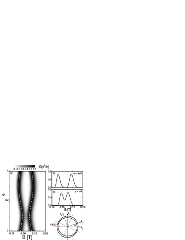
Figure 3: (a) Splitting of the first focusing peak as a function the crystallographic angle $\varphi$ for $E_{F}=23$meV, $m^{*}\!=\!0.055m_{0}$, $L=1.5\mu$m, $\alpha=15$meVnm, and $\beta/\alpha=1/3$. The dashed lines correspond to Eq. (9) and $B_{f}\!=\!165$mT; (b) and (c) show the focusing peaks for the minimum and maximum splitting; (d) scheme of the Fermi surface indicating the difference $\Delta k(\varphi)$.

III Splitting of the focusing peaks

III.1 Dependence with the crystal orientation

Figure 3 shows the splitting of the first focusing peak as a function of the crystal orientation (defined by the angle $\varphi$) with respect to the edge of the sample. The splitting shows a simple oscillatory behavior, whose angle dependence can be fully understood in terms of the shape of the Fermi surface and a simple semiclassical argument presented below. It is worth mentioning that the semiclassical description of the orbits is far from trivial in the presence of spin-orbit coupling.Littlejohn and Flynn (1992); Frisk and Guhr (1993); Amann and Brack (2002); Pletyukhov et al. (2002); Zaitsev (2002); Pletyukhov and Zaitsev (2003); Reynoso et al. (2004); Zülicke et al. (2007) In particular, in the presence of both Rashba and Dresselhaus couplings, there is an extra complication due to the possibility to have mode conversion points (points where the spin-orbit field cancels).Littlejohn and Flynn (1992); Frisk and Guhr (1993); Amann and Brack (2002); Pletyukhov et al. (2002); Zaitsev (2002); Pletyukhov and Zaitsev (2003) This will be important for the effect discussed in the following section.

Here, however, we can argue that the SO coupling is sufficiently strong so that the spin follows the momentum adiabatically. We can then use the usual semiclassical description for a band structure given by Eq. (3). In that case, the semiclassical equations of motion are given by

$$\dot{\bm{r}}\!=\!\bm{v}\!=\!\frac{1}{\hbar}\nabla_{\bm{k}}\varepsilon(\bm{k})\,,\qquad\dot{\bm{k}}\!=\!\frac{e}{\hbar c}\bm{v}\times\bm{B}\,.$$ (8)

For $\bm{B}\!=\!B\hat{z}$, the solution of these equations implies that $\bm{k}(t)$ moves along the Fermi surface while $\bm{r}(t)\!=\!\bm{r}(0)\!+\!\hat{z}\times\left(\bm{k}(t)\!-\!\bm{k}(0)\right)l_{c}^{2}$ and, as usual, the real-space orbit is related to the one in $k$-space by a $\pi/2$ rotation and a scale factor $l_{c}^{2}$. Since in our case there are two different Fermi surfaces, there are two real-space orbits whose radius difference is then given by $\Delta r(\varphi)\!=\!l_{c}^{2}\Delta k(\varphi)$ where $\Delta k(\varphi)=(2m^{*}/\hbar^{2})\sqrt{\alpha^{2}+\beta^{2}-2\alpha\beta\sin{2\varphi}}$ is the orientation-dependent difference of the two wave vectors of the two Fermi surfaces (see Fig 3). Here, in determining the cyclotron radius, we have neglected the fact that the velocity is not parallel to $\bm{k}$ (normal injection does not always correspond to $k_{y}=0$). In the limit $\Delta k(\varphi)/k_{F}\ll 1$, as it is the case here, this is an excellent approximation.

Then, the peak position is given by $B_{\pm}(\varphi)\!=\!B_{f}(\varphi)\pm\Delta B(\varphi)/2$, where $B_{f}(\varphi)\simeq\frac{2c}{eL}\sqrt{2Em^{*}}$ and

$$\Delta B(\varphi)=\frac{4m^{*}}{\hbar eL}\alpha\sqrt{1+\left(\frac{\beta}{\alpha}\right)^{2}-2\left(\frac{\beta}{\alpha}\right)\sin 2\varphi}$$ (9)

is the magnetic-field splitting of the first focusing peak. This is indicated in Fig. 3 with dashed lines.

The agreement with the exact numerical result is excellent, showing that the simplified semiclassical picture is very accurate in this regime. From Eq. (9), we see that a measure of the peak splitting is a direct way to measure $\alpha$ and $\beta$. One possible way to do it would be to use different sets of pairs of QPCs oriented in different angles with respect to the crystallographic axis.

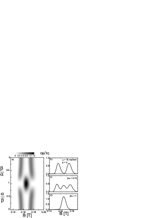
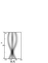
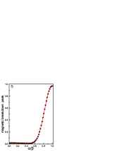
Figure 4: Magnetic breakdown between different cyclotron orbits. (a) Evolution of the first focusing peak as a function of $\alpha$ and $\beta$ when fixing the greater in $15$ meVnm. The splitting evolves as expected from Eq. (9) until the two coupling have similar values. Close to this point a third peak appears as a consequence of the quantum tunneling between the two orbits. For $\alpha\!=\!\beta$ we have only one orbit, $\Delta k\!=\!0$, and then only one peak; (b), (c) and (d) show the focusing peaks for different values of the SO coupling parameters; (e) focusing signal as a function of $\varphi$ for $\alpha/\beta=0.75$; (f) fitting of the amplitude of the central peak with Eq. (12).

III.2 Additional peak: ”magnetic breakdown”

Let us now consider a different situation where the crystallographic orientation is kept fixed (we take $x^{\prime}\!=\!x$ so that $\varphi\!=\!0$) but the magnitude of the spin-orbit coupling ($\alpha$ or $\beta$) is changed. This is shown in Fig. 4. When one of the SO couplings dominates the two peaks structure is clearly seen. Consider the case of small $\alpha/\beta$ in Fig. 4; as $\alpha/\beta$ increases the splitting also increases in agreement with Eq. (9). However, for $\alpha/\beta\simeq 1$, a third peak develops at $B=B_{f}$. The amplitude of this peak increases at the expenses of the other two and becomes the only peak for $\alpha\!=\!\beta$. The fact that there is only one peak when $\alpha\!=\!\beta$ is quite clear from the fact that in that case the two Fermi surfaces are circular and have the same radius.

The transition from two to three peaks can be understood in terms of tunneling between cyclotron orbits, in the same spirit as the magnetic breakdown between band orbits in bulk metals.Cohen and Falicov (1961) For $\alpha\simeq\beta$, the ”gap” in $k$-space between the two Fermi surfaces, that is the minimum distance between them $\Delta k_{-}\!=\!2m^{*}|\alpha\!-\!\beta|/\hbar^{2}$, is very small and the magnetic field can induce a tunneling transition between both orbits. Therefore, if $f(B-B^{*})$ describes a single focusing peak centered around $B^{*}$, the complete focusing signal is expected to behave as

$$\left(f(B-B_{+})\!+\!f(B-B_{-})\right)(1-p)+2p\,f(B-B_{f})\,,$$ (10)

where $p$ is the tunneling probability, which can be estimated using a Landau-Zener-type argument. Following Refs. [Shoenberg, 1984; de Andrada e Silva et al., 1994], a rough estimate for $p$ is

$$p=\exp\left(-\pi l_{c}^{2}\sqrt{\frac{\Delta k_{-}^{3}}{a+b}}\right)\,,$$ (11)

where $1/a$ and $1/b$ are the curvature radii of the two Fermi surfaces in the tunneling region, ie. close to the minimum gap point. For $\alpha/\beta\sim 1$, this can be approximated by

$$p=\exp\left(-\frac{\pi m^{*}k_{F}l_{c}^{2}}{\hbar^{2}}\frac{(\alpha-\beta)^{2}}{\sqrt{\alpha\beta}}\right)=\exp\left(-\gamma\frac{(x-1)^{2}}{\sqrt{x}}\right)$$ (12)

with $x=\alpha/\beta$ and $\gamma=\pi m^{*}k_{F}l_{c}^{2}\beta/\hbar^{2}$. This expression fits the numerical data [see Fig. 4f] up-to a factor of $0.6$ in $\gamma$. Notice that the fitting function is not a Gaussian and that $p$ is independent of the crystallographic angle $\varphi$; it only depends on the local properties of the Fermi surface around the minimum gap.

At this point it is worth mentioning that the magnetic breakdown of the cyclotron orbits has previously been used to explain the anomalous behavior of the magnetoresistance oscillations in systems with spin-orbit coupling.de Andrada e Silva et al. (1994) This interpretation has been challenged very recentlyWinkler et al. (2000); Keppeler and Winkler (2002); Winkler (2003) arguing that the dynamics of the spin cannot follow, in that case, the momentum. Our case, however, is different as we are in the strong spin-orbit limit and the magnetic breakdown interpretation is appropriate.

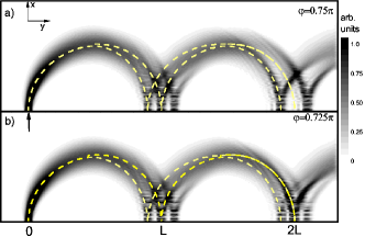
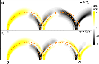
Figure 5: Imaging of the cyclotron orbits (see text). (a) and (b) show the total conductance $G_{\mathrm{inj,tip}}$ for two different crystallographic orientation, $\varphi=0.75\pi$ and $0.725\pi$, respectively, $\beta/\alpha=0.75$ and $L=1.5\mu$m. Note that in both cases there are three peaks at the first bounce against the edge of the sample while in the second bounce the central peak is missing (due to interference) only in (a); (c) and (d) show the spin resolved conductances, $G_{\mathrm{inj\uparrow,tip\uparrow}}-G_{\mathrm{inj\uparrow,tip\downarrow}}$. The absence of a sign change along the orbit is a signature of the magnetic breakdown.

In order to explicitly show the magnetic breakdown of the cyclotron orbits, we plot in Figs. 5a and 5b the conductance $G_{\mathrm{inj,tip}}$ from the injector to a conducting tip, located above the 2DEG, as a function of the tip position (see Ref. [Usaj and Balseiro, 2004] for details) and for two different crystallographic orientations, $\varphi=0.75\pi$ and $0.725\pi$, respectively. This essentially corresponds to calculate the probability for an electron injected through QPC $I$ to reach a given point in the 2DEG and hence brings information about the orbits followed by the electrons. The images obtained in this way are similar, although with a much better resolution, that the ones we would have obtained by simulating the presence of a tip as a scatterer (the experimental technique developed in Refs. [Topinka et al., 2000, 2001; Aidala et al., 2006, 2007]).

Although it is difficult to distinguish the orbits along the full path, three different orbits are apparent in both cases close to the first bouncing point, which correspond to the first focusing condition. As each of these orbits have a spin projection associated with it, we plot in Figs. 5c and 5d the difference between the spin resolved conductances, $G_{\mathrm{inj\uparrow,tip\uparrow}}-G_{\mathrm{inj\uparrow,tip\downarrow}}$, where the spin-quantization axis corresponds to $\hat{\bm{y}}$. This allows us to follow the direct orbits and the ones that involve tunneling. For this, it is important to take into account that for $\beta=0$, we would observe a change of sign of $G_{\mathrm{inj\uparrow,tip\uparrow}}-G_{\mathrm{inj\uparrow,tip\downarrow}}$ in the middle of the orbit as the spin rotates from $|\uparrow\rangle$ to $|\downarrow\rangle$. Here, the fact that there is an orbit in which this quantity does not change sign is an indication of the tunneling from one orbit to the other. To support this interpretation, we also show the semiclassical orbits (dashed lines) expected for an electron injected with a given spin polarization along the $y$ axis. To include the orbits that involve tunneling, we simply change from one orbit to the other at the position related to the minimum gap in $k$-space (see Fig. 7).

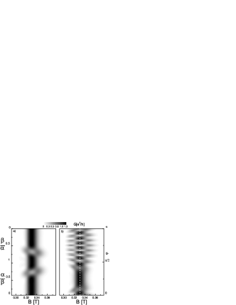
Figure 6: Focusing signal at the second focusing peak: (a) as a function of $\alpha$ ($\beta$) for $\beta(\alpha)=15$meVnm and $\varphi=0$. As expected there is only a single peak, except for $\alpha/\beta\simeq 0.75$ where there is a destructive interference between the different orbits shown in Fig. 7. Notice this point correspond to the case where there are three peaks at the first focusing condition; (b) as a function of the crystallographic angle $\varphi$ for $\alpha/\beta\simeq 0.75$.

An interesting effect occurs at the second focusing peak (second bounce in Fig. 5). In such a case, the peak structure results from the interference of several paths and hence destructive interference can results for particular values of the parameters. In particular, we see in Fig. 5 that for $\varphi=0.75\pi$ the central peak is missing. In order to understanding the origin of this effect, we show in Fig. 6a the focusing signal as a function of $\alpha/\beta$ for $\varphi=0$ and the same microscopic parameters as in Fig. 4. For almost all values of $\alpha/\beta$ there is a single peak (as in the $\beta=0$ case). However, for $\alpha/\beta\simeq 0.75$, when the first focusing peak shows a three peak structure (see Fig. 4), the central peak disappears while two satellites peaks emerge. When setting $\alpha/\beta=0.75$ this effect has an oscillatory behavior as a function of the crystal orientation. This is shown in Fig. 6b (see also Fig. 4(e) for a comparison with the first focusing peak structure).

As mentioned above, the origin of this modulation of the amplitude of the second focusing peak is the interference between the different orbits that contribute to the signal. These orbits, for an electron injected with its spin pointing along the $y$-axis, are shown in Fig. 7. The regions in real space where tunneling between the two orbits occurs are indicated with circles. The position of these regions depends on the crystal orientation. Figures 7a and 7b show the orbits that contribute to the central peak of the second focusing peak, while Fig. 7c shows the overlap of the two orbits. Figures 7d and 7e show the orbits that contribute to one of the satellites in the second focusing peak. The letters A,B,C and D identify the different locations of the bounces and then the different focusing peaks.

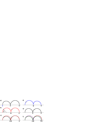
Figure 7: Semiclassical orbits (in real space) containing two bounces for an electron injected at the point indicated by the arrow with its spin polarized along the edge of sample. (a) Direct orbit (no tunneling) and (b) orbit with two tunneling events, indicated by the circles. Here $\tilde{\varphi}$ defines the angle where tunneling occurs; (c) superposition of orbits (a) and (b). Notice that after the second tunneling event the two orbits overlap; (d) and (e) orbits that involve one tunneling event; (f) superposition of all previous orbits. The letters A,B,C and D identify the different locations of the bounces.

As the phase acquired due to the tunneling between orbits is independent of $\varphi$, in order to account for the angle dependence of the interference pattern we need to include the orbital phase acquired by the electron along the different paths. In addition, we notice that after the second tunneling event the two orbits in Fig. 7c follow exactly the same path. Since they accumulate the same orbital phase from there to the next bouncing point, if they interfere destructively right after the tunneling, they will do it along the final part of the orbit. This is clearly seen in Fig. 5 where for $\varphi=0.75\pi$ the orbit corresponding to the central peak in the second focusing peak has disappeared completely after the second tunneling event.

The central peak amplitude is then given by

$$A=|\sqrt{P_{d}}+\sqrt{P_{t}}e^{\mathrm{i}(2\theta_{t}+\theta_{orb})}|^{2}$$ (13)

where $P_{d}$ and $P_{t}$ are the probability of the direct and tunneling paths, respectively [paths (a) and (b) in Fig. 7], $\theta_{t}$ is the phase acquired by the electron due to each tunneling event (we assume them to be equal), and $\theta_{orb}=\theta_{1}-\theta_{2}$ is the difference of the orbital phases of the two paths. In the semiclassical picture, the orbital phase of each path is given by $1/\hbar\int_{C}\bm{p}\cdot\mathrm{d}\bm{r}$, where the integral is done along the classical path $C$, $\bm{p}$ is the canonical momentum and $\bm{r}$ the position vector satisfying

$$\dot{\bm{r}}=\frac{\partial H}{\partial\bm{p}}\qquad\dot{\bm{p}}=-\frac{\partial H}{\partial\bm{r}}$$ (14)

In the strong spin-orbit limit, the Hamiltonian $H$ is given byAmann and Brack (2002); Pletyukhov and Zaitsev (2003); Zülicke et al. (2007)

$$H=\frac{P^{2}}{2m^{*}}\pm\sqrt{(\alpha P_{x^{\prime}}\!+\!\beta P_{y^{\prime}})^{2}\!+\!(\alpha P_{y^{\prime}}\!+\!\beta P_{x^{\prime}})^{2}}$$ (15)

with $\bm{P}=\bm{p}+(e/c)\bm{A}$. Using a symmetric gauge, it is straightforward to show that $1/\hbar\int_{C}\bm{p}\cdot\mathrm{d}\bm{r}=(1/2l_{c}^{2})\int r_{C}^{2}\mathrm{d}\phi$, where $r_{C}$ is the radius of the corresponding cyclotron orbit. The orbital phase difference between the two paths is then

$$\theta_{orb}=\frac{1}{2l_{c}^{2}}\left(\int_{0}^{\tilde{\varphi}}(r_{1}^{2}-r_{2}^{2})\,\mathrm{d}\phi-\int_{\tilde{\varphi}}^{\pi}(r_{1}^{2}-r_{2}^{2})\,\mathrm{d}\phi\right)$$ (16)

with $\tilde{\varphi}$ as the angle where tunneling occurs (see Fig. 7) and $r_{i}$, $i=1,2$, as the radii of the orbits. This integral can be calculated analytically for arbitrary values of $\alpha$ and $\beta$ in terms of elliptic integrals. However, for $\alpha/\beta\simeq 1$, it can be approximated by

$$\theta_{orb}=4l_{c}^{2}k_{F}\frac{2\sqrt{\alpha\beta}m^{*}}{\hbar^{2}}\cos(\varphi-\frac{\pi}{4}).$$ (17)

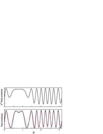
Figure 8: (a) Amplitude of the second focusing peak (indicated by a dashed line in Fig. 6) as a function of the crystallographic orientation. The oscillation is due to quantum interference between different paths (see Fig. 7); (b) same as above but without taking into account the contribution from the satellite peaks. The dashed (dotted) line corresponds to a fitting using the exact (approximated) value of $\theta_{orb}$, given by Eq. (16)[Eq. (17)].

Figure 8 shows the total central peak amplitude obtained numerically as a function of $\varphi$. Since for $\varphi\simeq\pi/4$ the satellite peaks merge into the central peak, in Fig. 8b we plot the central peak amplitude subtracting the satellite contributions. This can be done because the orbits that contribute to the central peak for all angles are those where the electron arrives with the same spin orientation it had at the injector. A fitting of the peak amplitude, using Eq. (13) with $P_{d}$ and $P_{t}$ as the only fitting parameters, is shown in Fig. 8b. The dotted line was obtained using the approximated expression for $\theta_{orb}$ [Eq. (17)], while the dashed line corresponds to the exact expression [Eq. (16)]. Once again, the agreement is very good, given further support to the magnetic breakdown interpretation.

It is easy to verify that for the case of the satellite peaks, $\theta_{orb}$ takes the same value than in the case of the central peak. However, as in this case both interfering paths contain a tunneling event, $\theta_{t}$ drops out. Then, the fact that there is destructive interference in the central peak when the satellites have there maximum values indicates that $\theta_{t}\simeq\pi/2$ as expected from the magnetic breakdown picture. In the above analysis, we did not consider explicitly the phase acquired by the spin degree of freedom. In general, such phase has a nontrivial dependence with the geometry of the orbit. Littlejohn and Flynn (1992); Frisk and Guhr (1993); Amann and Brack (2002); Pletyukhov et al. (2002); Zaitsev (2002); Pletyukhov and Zaitsev (2003) Here, since we assumed that the spin follows the SO field, that is, it rotates around the $z$ axis, this phase is not relevant. However, special care should be taken when considering the effect of the tunneling between orbits as the spin may have an additional rotation. As this case involves a mode conversion point, a semiclassical analysis of this phase is not simple— we are not aware of a simple way to estimate it. Therefore, the fact that our results indicate that the phase due to tunneling is just the usual $\pi/2$, is an indication that the spin phase is $0$ or $\pi$. Further work is needed to clarify this point.

IV Summary

We have shown that the interplay between the Rashba and Dresselhaus couplings introduces new effects on the transverse electron focusing. The most interesting aspect is the appearance of additional structure of the focusing peaks related to the magnetic breakdown of the cyclotron orbits when the two SO couplings have similar magnitude: the two sheets of the Fermi surface lead to different paths in real space and, as we have shown, the tunneling between different paths generates new structure in the focusing peaks. In addition, interference effects between these paths lead to an oscillatory behavior of the second focusing peak amplitude as a function of the orientation of the crystallographic axes. We have shown that the observed interference effects are dominated by the orbital phase accumulated along the different paths. This is so because in this regime, the spin adiabatically follows the momentum and the associated Berry phase cancels out while the spin phase due to tunneling seems to be irrelevant here. One could however envision a different regime where the spin dynamics would be important for which a deeper understanding of the spin dynamics during the tunneling as well as of the semiclassical description of the problem is needed.

The magnetic breakdown of the orbits as well as the interference effect could be directly observed using some of the techniques recently developed for imaging the electron flow. Topinka et al. (2000, 2001); Aidala et al. (2006); Reynoso et al. (2006b) In this work we have been mostly concerned with the dependence of the different effects on the crystal orientation. In practice, the experimental observation is a bit cumbersome as it requires us to tailor different QPC setups in different orientations. An alternative to this could be the use of in-plane magnetic fields to modulate $\Delta k_{-}$ as well as $k_{+}$ and $k_{-}$. For instance, for $\alpha\simeq\beta$, an in-plane field applied along the $\hat{x^{\prime}}-\hat{y^{\prime}}$ direction will essentially control the magnitude of the gap in $k$-space, and then the probability for tunneling. On the other hand, in-plane field along the $\hat{x^{\prime}}+\hat{y^{\prime}}$ direction can be used to modulate $k_{+}$ and $k_{-}$ and then the interference pattern. This also have the advantage of keeping $k_{+}+k_{-}$ constant and then the focusing condition.

Finally, it is interesting to note that while the splitting of the focusing peaks allows for the spatial separation of the spin components as in a Stern-Gerlach device,Usaj and Balseiro (2004); Rokhinson et al. (2004) the presence of the magnetic breakdown between orbits provides a way to separate a given spin component in a superposition of two spatially separated orbits.

V Acknowledgments

This work was supported by ANPCyT Grants N^o13829, 13476, 2006-483 and CONICET PIP 5254. A.A.R. and G.U. acknowledge support from CONICET.

References

- Awschalom et al. (2002) D. Awschalom, N. Samarth, and D. Loss, eds., Semiconductor Spintronics and Quantum Computation (Springer, New York, 2002).
- Datta and Das (1990) S. Datta and B. Das, Appl. Phys. Lett. 56, 665 (1990).
- Schliemann et al. (2003) J. Schliemann, J. C. Egues, and D. Loss, Phys. Rev. Lett. 90, 146801 (2003).
- König et al. (2006) M. König, A. Tschetschetkin, E. M. Hankiewicz, J. Sinova, V. Hock, V. Daumer, M. Schäfer, C. R. Becker, H. Buhmann, and L. W. Molenkamp, Phys. Rev. Lett. 96, 076804 (2006).
- Kovalev et al. (2007) A. A. Kovalev, M. F. Borunda, T. Jungwirth, L. W. Molenkamp, and J. Sinova, Phys. Rev. B 76, 125307 (2007).
- Dyakonov and Perel (1971) M. I. Dyakonov and V. I. Perel, JETP Lett. 13, 467 (1971), ;M. I. Dyakonov, Phys. Lett. A 35, 459 (1971).
- Hirsch (1999) J. E. Hirsch, Phys. Rev. Lett. 83, 1834 (1999).
- Murakami et al. (2003) S. Murakami, N. Nagaosa, and S. C. Zhang, Science 301, 1348 (2003).
- Sinova et al. (2004) J. Sinova, D. Culcer, Q. Niu, N. A. Sinitsyn, T. Jungwirth, and A. H. MacDonald, Phys. Rev. Lett. 92, 126603 (2004).
- Kato et al. (2004) Y. K. Kato, R. C. Myers, A. C. Gossard, and D. D. Awshalom, Science 306, 1910 (2004).
- Usaj and Balseiro (2005) G. Usaj and C. A. Balseiro, Europhys. Lett. 72, 631 (2005).
- Wunderlich et al. (2005) J. Wunderlich, B. Kaestner, J. Sinova, and T. Jungwirth, Phys. Rev. Lett. 94, 047204 (2005).
- Kato et al. (2005) Y. K. Kato, R. C. Myers, A. C. Gossard, and D. D. Awschalom, Appl. Phys. Lett. 87, 022503 (2005).
- Sih et al. (2005) V. Sih, R. C. Myers, Y. K. Kato, W. H. Lau, A. C. Gossard, and D. D. Awschalom, Nat. Phys. 1 p. 31 (2005).
- Nikolic et al. (2005) B. K. Nikolic, S. Souma, L. P. Zarbo, and J. Sinova, Phys. Rev. Lett. 95, 046601 (2005).
- Nomura et al. (2005a) K. Nomura, J. Wunderlich, J. Sinova, B. Kaestner, A. H. MacDonald, and T. Jungwirth, Phys. Rev. B 72, 245330 (2005a).
- Engel et al. (2005) H.-A. Engel, B. I. Halperin, and E. I. Rashba, Phys. Rev. Lett. 95, 166605 (2005).
- Erlingsson and Loss (2005) S. I. Erlingsson and D. Loss, Phys. Rev. B 72, 121310(R) (2005).
- Nomura et al. (2005b) K. Nomura, J. Sinova, T. Jungwirth, Q. Niu, and A. H. MacDonald, Phys. Rev. B 71, 041304(R) (2005b).
- Adagideli and Bauer (2005) I. Adagideli and G. E. W. Bauer, Appl. Phys. Lett. 95, 256602 (2005).
- Reynoso et al. (2006a) A. Reynoso, G. Usaj, and C. A. Balseiro, Phys. Rev. B 73, 115342 (2006a).
- Winkler (2003) R. Winkler, Spin-orbit coupling effects in two-dimensional electron and hole systems (Springer-Verlag, 2003).
- Nitta et al. (1997) J. Nitta, T. Akazaki, H. Takayanagi, and T. Enoki, Phys. Rev. Lett. 78, 1335 (1997).
- Ganichev et al. (2004) S. D. Ganichev, V. V. Bel’kov, L. E. Golub, E. L. Ivchenko, P. Schneider, S. Giglberger, J. Eroms, J. De Boeck, G. Borghs, W. Wegscheider, D. Weiss and W. Prettl, Phys. Rev. Lett. 92, 256601 (2004).
- Giglberger et al. (2007) S. Giglberger, L. E. Golub, V. V. Bel’kov, S. N. Danilov, D. Schuh, C. Gerl, F. Rohlfing, J. Stahl, W. Wegscheider, D. Weiss, W. Prettl, and S. D. Ganichev, Phys. Rev. B 75, 035327 (2007).
- Miller et al. (2003) J. B. Miller, D. M. Zumbühl, C. M. Marcus, Y. B. Lyanda-Geller, D. Goldhaber-Gordon, K. Campman, and A. C. Gossard, Phys. Rev. Lett. 90, 076807 (2003).
- Meier et al. (2007) L. Meier, G. Salis, I. Shorubalko, E. Gini, S. Sch n, and K. Ensslin, Nat. Phys. 3, 650 (2007).
- Meier et al. (2008) L. Meier, G. Salis, E. Gini, I. Shorubalko, and K. Ensslin, Phys. Rev. B 77, 035305 (2008).
- Bernevig et al. (2006) B. A. Bernevig, J. Orenstein, and S.-C. Zhang, Phys. Rev. Lett. 97, 236601 (2006).
- Weber et al. (2007) C. P. Weber, J. Orenstein, B. A. Bernevig, S.-C. Zhang, J. Stephens, and D. D. Awschalom, Phys. Rev. Lett. 98, 076604 (2007).
- Frolov et al. (2008) S. Frolov, A. Venkatesan, W. Yu, S. Luescher, W. Wegscheider, and J. Folk (2008), arXiv:0801.4021v3 [cond-mat.mes-hall].
- van Houten et al. (1989) H. van Houten, C. W. J. Beenakker, J. G. Willianson, M. E. I. Broekaart, P. H. M. vanLoosdrecht, B. J. van Wees, J. E. Mooji, C. T. Foxon, and J. J. Harris, Phys. Rev. B 39, 8556 (1989).
- Beenakker and van Houten (1991) C. W. Beenakker and H. van Houten, in Solid State Physics, edited by H. Eherenreich and D. Turnbull (Academic Press, Boston, 1991), vol. 44, pp. 1–228.
- Usaj and Balseiro (2004) G. Usaj and C. A. Balseiro, Phys. Rev. B 70, 041301(R) (2004).
- Rokhinson et al. (2004) L. P. Rokhinson, V. Larkina, Y. B. Lyanda-Geller, L. N. Pfeiffer, and K. W. West, Phys. Rev. Lett. 93, 146601 (2004).
- Dedigama et al. (2006) A. Dedigama, D. Deen, S. Murphy, N. Goel, J. Keay, M. Santos, K. Suzuki, S. Miyashita, and Y. Hirayama, Physica E 34, 647 (2006).
- Reynoso et al. (2004) A. Reynoso, G. Usaj, M. J. Sanchez, and C. A. Balseiro, Phys. Rev. B 70, 235344 (2004).
- Zülicke et al. (2007) U. Zülicke, J. Bolte, and R. Winkler, New J. Phys. 9, 355 (2007).
- Schliemann (2008) J. Schliemann, Phys. Rev. B 77, 125303 (2008).
- Cohen and Falicov (1961) M. H. Cohen and L. M. Falicov, Phys. Rev. Lett. 7, 231 (1961).
- de Andrada e Silva et al. (1994) E. A. de Andrada e Silva, G. C. La Rocca, and F. Bassani, Phys. Rev. B 50, 8523 (1994).
- Topinka et al. (2000) M. Topinka, B. LeRoy, S. Shaw, E. Heller, R. Westervelt, K. Maranowski, and A. Gossard, Science 289, 2323 (2000).
- Topinka et al. (2001) M. Topinka, B. LeRoy, R. Westervelt, S. Shaw, R.Fleischmann, E. Heller, K. Maranowski, and A. Gossard, Nature 410, 183 (2001).
- Aidala et al. (2006) K. E. Aidala, R. E. Parrott, E. Heller, and R. Westervelt, Physica E 34, 409 (2006).
- Reynoso et al. (2006b) A. Reynoso, G. Usaj, and C. A. Balseiro, in Quantum Magnetism, NATO Science for Peace and Security Series, pp.151-162, Springer (2008); arXiv:cond-mat/0703267v2.
- Aidala et al. (2007) K. E. Aidala, R. E. Parrott, T. Kramer, E. J. Heller, R. M. Westervelt, M. P. Hanson, and A. C. Gossard, Nat. Phys. 3, 464 (2007).
- Schliemann and Loss (2003) J. Schliemann and D. Loss, Phys. Rev. B 68, 165311 (2003).
- Mishchenko and Halperin (2003) E. G. Mishchenko and B. I. Halperin, Phys. Rev. B 68, 045317 (2003).
- Zarea and Ulloa (2005) M. Zarea and S. E. Ulloa, prb 72, 085342 (pages 5) (2005).
- Zhang (2006) D. Zhang, J. Phys. A: Math. and Gen. 39, L477 (2006).
- Bychkov and Rashba (1984) Y. A. Bychkov and E. I. Rashba, JETP Letters 39, 78 (1984).
- Pletyukhov et al. (2002) M. Pletyukhov, C. Amann, M. Mehta, and M. Brack, Phys. Rev. Lett. 89, 116601 (2002).
- Tsoi (1975) V. S. Tsoi, JETP Lett. 22, 197 (1975).
- Potok et al. (2002) R. M. Potok, J. A. Folk, C. M. Marcus, and V. Umansky, Phys. Rev. Lett. 89, 266602 (2002).
- Littlejohn and Flynn (1992) R. G. Littlejohn and W. G. Flynn, Phys. Rev. A 45, 7697 (1992).
- Frisk and Guhr (1993) H. Frisk and T. Guhr, Ann. Phys. 221, 229 (1993).
- Amann and Brack (2002) C. Amann and M. Brack, J. Phys. A: Math. and Gen. 35, 6009 (2002).
- Zaitsev (2002) O. Zaitsev, J. Phys. A: Math. and Gen. 35, L721 (2002).
- Pletyukhov and Zaitsev (2003) M. Pletyukhov and O. Zaitsev, J. Phys. A: Math. and Gen. 36, 5181 (2003).
- Rokhinson et al. (2006) L. P. Rokhinson, L. N. Pfeiffer, and K. W. West, Phys. Rev. Lett. 96, 156602 (2006).
- Reynoso et al. (2007) A. Reynoso, G. Usaj, and C. A. Balseiro, Phys. Rev. B 75, 085321 (2007).
- Eto et al. (2005) M. Eto, T. Hayashi, and Y. Kurotani, J. Phys. Soc. Jpn. 74, 1934 (2005).
- Ferry and Goodnick (1997) D. K. Ferry and S. M. Goodnick, Transport in Nanostructures (Cambridge University Press, New York, 1997).
- Shoenberg (1984) D. Shoenberg, Magnetic Oscillations in Metals (Cambridge University Press, Cambridge, England, 1984).
- Winkler et al. (2000) R. Winkler, S. J. Papadakis, E. P. De Poortere, and M. Shayegan, Phys. Rev. Lett. 84, 713 (2000).
- Keppeler and Winkler (2002) S. Keppeler and R. Winkler, Phys. Rev. Lett. 88, 046401 (2002).