Are Copying and Innovation Enough?

Abstract

Exact analytic solutions and various numerical results for the rewiring of bipartite networks are discussed. An interpretation in terms of copying and innovation processes make this relevant in a wide variety of physical contexts. These include Urn models and Voter models, and our results are also relevant to some studies of Cultural Transmission, the Minority Game and some models of ecology.

Introduction

There are many situations where an ‘individual’ chooses only one of many ‘artifacts’ but where their choice depends in part on the current choices of the community. Names for new babies and registration rates of pedigree dogs often reflect current popular choices HB03 ; HBH04 . The allele for a particular gene carried (‘chosen’) by an individual reflects current gene frequencies E04 . In Urn models the probabilities controlling the urn chosen by a ball can reflect earlier choices GL02 . In all cases copying the state of a neighbour, as defined by a network of the individuals, is a common process because it can be implemented without any global information ES05 . At the other extreme, an individual might might pick an artifact at random.

The Basic Model

We first consider a non-growing bipartite network in which $E$ ‘individual’ vertices are each attached by a single edge to one of $N$ ‘artifact’ vertices. At each time step we choose to rewire the artifact end of one edge, the departure artifact chosen with probability $\Pi_{R}$. This is attached to an arrival artifact chosen with probability $\Pi_{A}$. Only after both choices are made is the graph rewired as shown in Fig. 1.

[width=0.5]copymodel3ind.eps

Figure 1: The bipartite network of $E$ individual vertices, each connected by a single edge (solid lines) to any one of $N$ artifacts. The dashed lines below the individuals are a social network. In the event shown individual 3 updates their choice, making B the departure artifact. They do this by copying the choice of a friend, friend of a friend, etc., found by making a random walk on the social network. Here this produces A as the arrival artifact so edge 3B is rewired to become edge 3A.

The degree distribution of the artifacts when averaged over many runs of this model, $n(k,t)$, satisfies the following equation:-

$$n(k,t+1) = n(k,t)+n(k+1,t)\Pi_{R}(k+1,t)\left(1-\Pi_{A}(k+1,t)\right)$$ (1)

$$-n(k,t)\Pi_{R}(k,t)\left(1-\Pi_{A}(k,t)\right)-n(k,t)\Pi_{A}(k,t)\left(1-\Pi_{R}(k,t)\right)$$

$$+n(k-1,t)\Pi_{A}(k-1,t)\left(1-\Pi_{R}(k-1,t)\right),\;\;\;(E\geq k\geq 0)\,,$$

where $n(k)=\Pi_{R}(k)=\Pi_{A}(k)=0$ for $k=-1,(E+1)$. If $\Pi_{R}$ or $\Pi_{A}$ have terms proportional to $k^{\beta}$ then this equation is exact only when $\beta=0$ or $1$ EP07 . We will use the most general $\Pi_{R}$ and $\Pi_{A}$ for which (1) is exact, namely

$$\Pi_{R}=\frac{k}{E},\qquad\Pi_{A}=p_{r}\frac{1}{N}+p_{p}\frac{k}{E},\qquad p_{p}+p_{r}=1\qquad(E\geq k\geq 0)\;.$$ (2)

This is equivalent to using a complete graph with self loops for the social network at this stage but these preferential attachment forms emerge naturally when using a random walk on a general network ES05 . This choice for $\Pi_{A}$ has two other special properties: one involves the scaling properties EP07 and the second is that these exact equations can be solved analytically Evans07 ; EP07 ; EP07eccs07 ; Evans07pisa . The generating function $G(z,t)=\sum_{k}z^{k}n(k,t)$ is decomposed into eigenmodes $G^{(m)}(z)$ through $G(z,t)=\sum_{m=0}^{E}c_{m}(\lambda_{m})^{t}G^{(m)}(z)$. From (1) we find a second order linear differential equation for each of the eigenmodes with solution EP07

$$G^{(m)}(z) = (1-z)^{m}{}_{2}F_{1}(a+m,-E+m;1-E-a(N-1);z)\,,\;\;\;a=\frac{p_{r}}{p_{p}}\frac{E^{\prime}}{N}\,,$$

$${}\lambda_{m} = 1-m(m-1)\frac{p_{p}}{EE^{\prime}}-m\frac{p_{r}}{E},\qquad 0\leq m\leq E\;,$$ (3)

where $E^{\prime}=E$. These solutions are well known in theoretical population genetics as those of the Moran model E04 and one may map the bipartite model directly onto a simple model of the genetics of a haploid population EP07 .

The equilibrium result for the degree distribution Evans07 ; EP07 is proportional to $\frac{\Gamma\left(k+a\right)}{\Gamma\left(k+1\right)}\frac{\Gamma\left(E+a(N-1)-1-k\right)}{\Gamma\left(E+1-k\right)}$. This has three typical regions. We have a condensate, where most of the edges are attached to one artifact $p(k=E)\sim O(N^{0})$, for $p_{r}\ll(E+1-\langle k\rangle)^{-1}$ . On the other hand when $p_{r}\gg(1+\langle k\rangle)^{-1}$ we get a peak at small $k$ with an exponential fall off, a distribution which becomes an exact binomial at $p_{r}=1$. In between we get a power law with an exponential cutoff, $p(k)\propto(k)^{-\gamma}\exp\{-\zeta k\}$ where $\gamma\approx(1-\frac{p_{r}}{p_{p}}\langle k\rangle)$ and $\zeta\approx-\ln(1-p_{r})$. For many parameter values the power $\gamma$ will be indistinguishable from one and this is a characteristic signal of an underlying copying mechanism seen in a diverse range of situations (e.g. see ATBK04 ; LJ06b ).

[width=0.5]CMni100na100k1prVARIOUSv2.eps

Figure 2: The equilibrium degree probability distribution function $p(k)=n(k)/N$ for $N=E=100$. Shown are (from top to bottom at low $k$) $p_{r}=1$ (red crosses), $10/E$ (green circles), $1/E$ (blue stars) and $0.1/E$ (magenta squares).

One of the best ways to study the evolution of the degree distribution EP07 ; EP07eccs07 is through the Homogeneity Measures, $F_{n}$. This is the probability that $n$ distinct edges chosen at random are connected to same artifact, and is given by $F_{n}(t):=(\Gamma(E+1-n)/\Gamma(E+1))(d^{n}G(z,t)/dz^{n})_{z=1}$. Further, each $F_{n}$ depends only on the modes numbered $0$ to $n$ so they provide a practical way to fix the constants $c_{n}$ in the mode expansion. Since $F_{0}=E$ and $F_{1}=1$, we find $c_{0}=1$ and $c_{1}=0$ while equilibration occurs on a time scale of $\tau_{2}=-1/\ln(\lambda_{2})$.

[width=0.5]Fnnina100pr0_01.eps

Figure 3: Plots of various $F_{n}(t)$ for $E=N=100$, $p_{r}=0.01$. The points are averages over $10^{5}$ runs while the lines are the exact theoretical results. From top to bottom we have: $F_{2}(t)$ (crosses), $F_{3}(t)$ (circles), $F_{4}(t)$ (stars).

Communities

Our first generalisation of the basic model is to consider two distinct communities of individuals, say $E_{x}$ ($E_{y}$) of type X (Y). The individuals of type X can now copy the choices made by their own community X with probability $p_{pxx}$, but a different rate is used when an X copies the choice made by somebody in community Y, $p_{pxy}$. An X individual will then innovate with probability $(1-p_{pxx}-p_{pxy})$. Another two independent copying probabilities can be set for the Y community. At each time step we choose to update the choice of a member of community X (Y) community with probability $p_{x}$ ($1-p_{x}$). Complete solutions are not available but one can find exact solutions for the lowest order Homogeneity measures and eigenvalues using similar techniques to those discussed above. The unilluminating details are given in EP07eccs07 .

Complex Social Networks

An obvious generalisation is to use a complex network as the Individual’s social network EP07eccs07 . When copying, done with probability $p_{p}$, an individual does a random walk on the social network to choose another individual and finally to copy their choice of artifact, as shown in Fig. 1. The random walk is an entirely local process, no global knowledge of the social network is needed, so it is likely to be a good approximation of many processes found in the real world. It also produces an attachment probability which is, to a good approximation, proportional to the degree distribution ES05 . The alternative process of innovation, followed with probability $p_{r}$, involves global knowledge through its normalisation $N$ in (2). However when $N\gg E$ this can represent innovation of new artifacts as it is likely that the arrival artifact has never been chosen before. However this process could also be a first approximation for other unknown processes used for artifact choice.

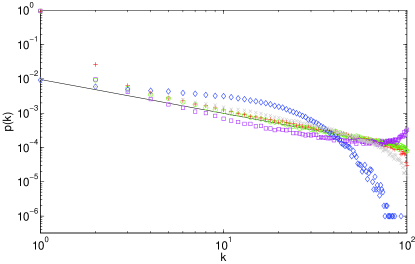
Figure 4: The degree distributions $p(k)$ averaged over $10^{4}$ runs for different social networks of average degree of 4: Erdős-Réyni (red pluses), Exponential (random with $p(k)\propto\exp(-\zeta k)$, green circles), Scale Free (random with $p(k)\propto k^{-3}$, purple squares), periodic lattices of two (grey crosses) and one (blue diamonds) dimension. The line is the analytic result where the social network is a complete graph with self loops. $N=E=100$, $p_{r}=1/E$.

Results shown in Fig.4 show that the existence of hubs in the Scale Free social network enhances the condensate while large distances in the social networks, as with the lattices, suppress the condensate.

An interesting example is the case of $N=2$ which is a Voter Model Liggett99 with noise (innovation $p_{r}\neq 0$) added. One can then compare the probability that a neighbour has a different artifact (the interface density) $\rho(t)$, a local measure of the inhomogeneity, with our global measure $(1-F_{2}(t))$. These coincide when the social network is a complete graph. However as we move from 3D to 1D lattices, keeping $N$, $E$ and $p_{r}$ constant, we see from Fig. 5 that both these local and global measures move away from the result for the complete graph but in opposite directions EP07eccs07 .

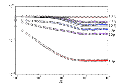
Figure 5: Inhomogeneity measures for various lattices against $t/E$. The black solid line represents the analytic result $(1-F_{2}(t))$ for $N=2$, $p_{r}=1/E$ and $E=729$. Numerical results for $(1-F_{2}(t))$ (triangles) and for the average probability that a neighbour has a different artifact, $rho(t)$ (circles) shown for social networks which are lattices of different dimensions. Averaged over $1000$ runs.

Different Update Methods

Another way we can change the model is to change the nature of the update. Suppose we first select the edge to be rewired and immediately remove it. Then, based on this network of $E^{\prime}=(E-1)$ edges, we choose the arrival artifact with probability $\Pi_{A}=(p_{r}/N)+(1-p_{r})k/E^{\prime}$. The original master equation (1) is still valid and exact. Moreover it can still be solved exactly giving exactly the same form as before, (3), but with $E^{\prime}=(E-1)$ not $E$. This gives very small differences of order $O(E^{-1})$ when compared to the original simultaneous update used initially.

Instead we will consider the simultaneous rewiring of $X$ edges in our bipartite graph at each step. We will choose the individuals, whose edges define the departure artifacts, in one of two ways: either sequentially or at random. The arrival artifacts will be chosen as before using $\Pi_{A}$ of (2).

The opposite extreme from the single edge rewiring case we started with ($X=1$) is the one where all the edges are rewired at the same time, $X=E$. This is the model used in HB03 ; HBH04 ; BLHH07 to model various data sets on cultural transmission. It is also the classic Fisher-Wright model of population genetics E04 . From this each homogeneity measure $F_{n}$ and the $n$-th eigenvector $\lambda_{n}$ may be calculated in terms of lower order results $F_{m}$ ($m<n$). Non trivial information again comes first from $F_{2}(t)=F_{2}(\infty)+(\lambda_{2})^{t}\left(F_{2}(0)-F_{2}(\infty)\right)$ where

$$F_{2}(\infty) = \frac{p_{p}^{2}+(1-p_{p}^{2})\langle k\rangle}{p_{p}^{2}+(1-p_{p}^{2})E}\,,\qquad\lambda_{2}=\frac{p_{p}^{2}(E-1)}{E}\,.$$ (4)

Comparing with the results for $X=1$ we see that there are large differences in the equilibrium solution and in the rate at which this is approached (measured in terms of number of the rewirings made). For intermediate values of $X$ we have not obtained any analytical results so for these numerical simulations are needed, as shown in Fig.6.

Figure 6: $\tau_{2}=-1/\ln(\lambda_{2})$ (left) and $F_{2}(\infty)$ (right) obtained by fitting $A+B(\lambda_{2})^{t}$ to the data for $F_{2}(t)$. For sequential ($m=4$ black circles, lower lines) and random ($m=6$ red triangles, upper lines) updates of $X$ individuals at a time. $N=E=100$, $p_{r}=1/E=0.01$ and averaged over $10^{4}$ runs. The dashed lines represent the best linear fit with $\tau_{2}\approx 1230(20)+21.8(3)X$ for $m=4$ and $\tau_{2}\approx 2470(10)+8.1(2)X$ for $m=6$. Theoretical values are $\tau_{2}\approx 2512.1$ and $F_{2}(\infty)\approx 0.50251$ for $X=1$ random update and $\tau_{2}\approx 3316.6$ and $F_{2}(\infty)\approx 0.33669$ for $X=100$ either update.

Supplementary Material

This following material is not part of the published paper.

Fig.7 shows the basic model — simultaneous rewiring of the artifact end of a single edge.

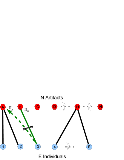
Figure 7: Each of $E$ ‘individual’ vertices is connected by a single edge to one of $N$ ‘artifact’ vertices. In the simplest model the artifact end of one edge is rewired at each time step. The edge to be rewired is chosen with probability $\Pi_{R}$ (the edge from individual $3$ to the departure artifact D). At the same time the arrival artifact is chosen with probability $\Pi_{A}$ (here labelled A). The rewiring is performed only after both choices have been made.

The evolution equation when $X$ edges are rewired simultaneously, as shown in Fig.8, is

$$G(z,t+E) = \sum_{k^{\prime}=0}^{E}[1+(z-1)\Pi_{\mathrm{A}}(k^{\prime})]^{E}n(k^{\prime},t)\,.$$ (5)

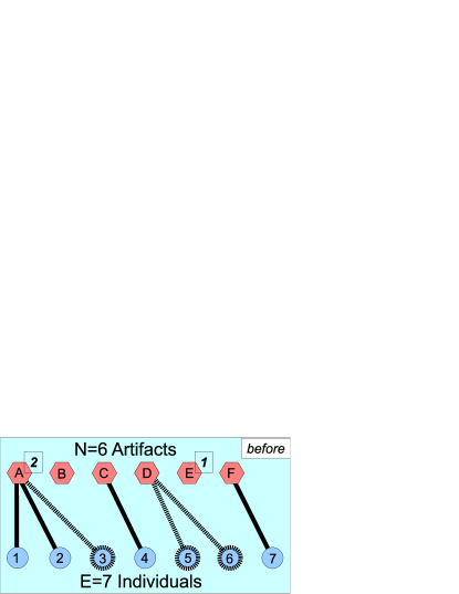
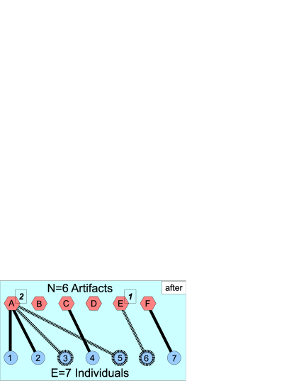
Figure 8: An example of the rewiring of the bipartite graph. Here the choice made by each of the $E=7$ ‘individual’ vertices is represented by an edge connected to one of the $N=6$ ‘artifact’ vertices. At each time step $X$ individuals decide to change their choice. Here $X=3$ and the chosen individuals (3,5, and 6) and their edges are indicated by dashed lines in the left hand panel. The new artifacts for the $X$ individuals are chosen with probability $\Pi_{A}$. Here A is chosen twice and E once and the result is shown on the right.

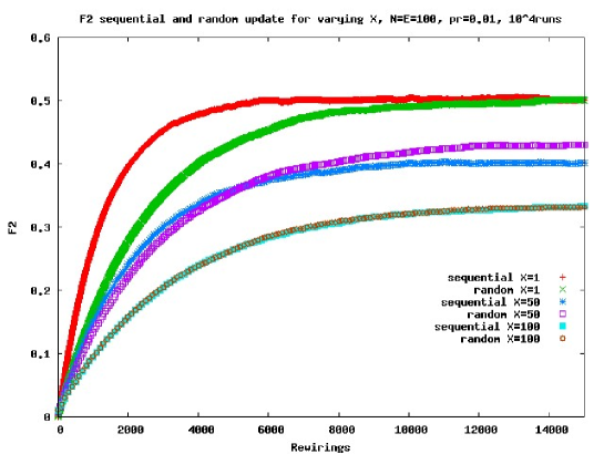
Figure 9: $F_{2}$ for sequential and random updates of $X$ individuals at a time. $N=E=100$, $p_{r}=1/E$ and averaged over $10^{4}$ runs.

For the values used in Fig. 6 and 9, we would predict $F_{2}(X=100;\infty)=0.3367\approx(1/3)+O(1/E)$ while $F_{2}(\mathrm{Rand},X=1;\infty)=0.5025\approx(1/2)+O(1/E)$. These clearly match the numerical results shown in Fig. 6 and 9.

Summary

We have shown how simple models of bipartite network rewiring can be solved exactly. The preferential attachment can be seen as emerging from simple copying using local information only on the social network. On the other hand the large $N$ limit shows the random attachment process may be thought of as innovation. Many other models can be mapped to this simple network model — see the review in EP07 . Thus copying and innovation may be enough to explain the results seen in many other contexts. such as the Minority game ATBK04 and in models of evolution LJ06b .

References

- (1) M. Anghel, Zoltan Toroczkai, Kevin E. Bassler, and G. Korniss, Competition in social networks: Emergence of a scale-free leadership structure and collective efficiency, Phys.Rev.Lett. 92 (2003) 058701.
- (2) R.A. Bentley, Carl P. Lipo, Harold A. Herzog, and Matthew W. Hahn, Regular rates of popular culture change reflect random copying, Evolution and Human Behavior 28 (2007) 151.
- (3) T.S. Evans, Exact solutions for network rewiring models, Eur. Phys. J. B 56 (2007) 65.
- (4) T.S. Evans, Randomness and complexity in networks, arXiv:0711.0603.
- (5) T.S. Evans and A.D.K. Plato, Exact solution for the time evolution of network rewiring models, Phys.Rev. E 75 (2007) 056101.
- (6) T.S. Evans and A.D.K. Plato, Network rewiring models, Networks and Heterogeneous Media 3 (2008) 221 [arXiv:0707.3783].
- (7) T.S. Evans and J.P. Saramäki, Scale free networks from self-organisation, Phys.Rev. E 72 (2005) 026138 [cond-mat/0411390].
- (8) W.J. Ewens, Mathematical population genetics: I. theoretical introduction, 2nd ed., Springer-Verlag New York Inc., 2004.
- (9) C. Godreche and J.M. Luck, Nonequilibrium dynamics of urn models, J. of Phys.Cond.Matter 14 (2002) 1601.
- (10) M.W. Hahn and R.A. Bentley, Drift as a mechanism for cultural change: an example from baby names, Proc.R.Soc.Lon. B 270 (2003) s120.
- (11) H.A. Herzog, R.A. Bentley, and M.W. Hahn, Random drift and large shifts in popularity of dog breeds, Proc.R.Soc.Lon B (Suppl.) 271 (2004) s353.
- (12) S. Laird and H.J. Jensen, A non-growth network model with exponential and 1/k scale-free degree distributions, Europhysics Letters 76 (2006) 710.
- (13) T.M. Liggett, Stochastic interacting systems: Contact, voter and exclusion processes, Springer-Verlag, New York, 1999.