Tombaugh 2: The First Open Cluster with a Significant Abundance Spread or Embedded in a Cold Stellar Stream?

Abstract

We present new high resolution spectroscopy from which we derive abundances and radial velocities for stars in the field of the open cluster Tombaugh 2, which has been suggested to be one of a group of clusters previously identified with the Galactic Anticenter Stellar Structure (also known as the Monoceros stream). Using VLT/FLAMES with the UVES and GIRAFFE spectrographs, we find a radial velocity (RV) of $\langle V_{r}\rangle=121\pm 0.4$ km s^-1 using eighteen Tombaugh 2 cluster stars; this is in agreement with previous studies, but at higher precision. We also make the first measurement of Tombaugh 2’s velocity dispersion, which is $\sigma_{int}=1.8\pm 0.3$ km s^-1. Our abundance analysis of RV-selected members finds that Tombaugh 2 is more metal-rich than previous studies have found; moreover, unlike the previous work, our larger sample also reveals that stars with the velocity of the cluster show a relatively large spread in chemical properties (e.g., $\Delta$[Fe/H] $>0.2$). This is the first time a possible abundance spread has been observed in an open cluster, though this is one of several possible explanations for our observations. While there is an apparent trend of [$\alpha$/Fe] with [Fe/H], the distribution of abundances of these “RV cluster members” also may hint at a possible division into two primary groups with different mean chemical characteristics — namely ($\langle$[Fe/H]$\rangle$, $\langle$[Ti/Fe]$\rangle$) $\sim$ ($-$0.06, $+$0.02) and ($-$0.28, $+$0.36). Isochrone fitting to the colour-magnitude distribution of apparent Tombaugh 2 members yields an age of 2.0 Gyr, $E(B-V)=0.3$, and $(m-M)_{0}=14.5$ or $d=7.9$ kpc for both populations — parameters that are within the range of previous findings. Based on position and kinematics Tombaugh 2 is a likely member of the GASS/Monoceros stream, which makes Tombaugh 2 the second star cluster within the originally proposed GASS/Monoceros family after NGC2808 to show some evidence for internal population dispersions. However, we explore other possible explanations for the observed spread in abundances and two possible sub-populations, with the most likely explanation being that the metal-poor ([Fe/H] = $-$0.28), more centrally-concentrated population being the true Tombaugh 2 clusters stars and the metal-rich ([Fe/H] = $-$0.06) population being an overlapping, and kinematically associated, but “cold” ($\sigma_{V}<2$ km s^-1) stellar stream at $R_{gc}\geq 15$ kpc.

1 Introduction

Tombaugh 2 (To2; at Galactic coordinates [$l,b$] = [232.8,$-$6.9]^∘) is an old, distant open cluster in the outer Galactic disc. We originally targeted this cluster as part of an ongoing program (e.g., Carraro et al., 2007) to explore in depth a set of star clusters proposed by Frinchaboy et al. (2004) — on the basis of their position and kinematics — to be possibly associated with the Monoceros stream (Mon; Newberg et al. 2002, Ibata et al. 2003, Yanny et al. 2003), also known as the Galactic anticenter stellar structure (GASS; Rocha-Pinto et al 2003, Crane et al. 2003). GASS/Mon was discovered as an overdensity of stars near the Galactic plane that seems to wrap around the outer parts of the Galactic disc and is frequently explained as tidal debris from the disruption of a dwarf galaxy on a low inclination orbit (e.g., Crane et al. 2003, Yanny et al. 2003, Penarrubia et al. 2005). To2 has also been associated with the reputed dwarf galaxy in Canis Major (CMa; Bellazzini et al. 2004), which is suggested to be a progenitor of the Mon/GASS structure (Martin et al. 2004a). However, Rocha-Pinto et al. (2006) argue that a more likely progenitor of Mon/GASS may lie somewhere in the region of the sky covered by the former constellation Argo Navis, and that the overdensity reported near CMa is correlated to a window in the dust extinction there; in this case, To2 would be farther displaced from the putative Mon/GASS progenitor. In any of these circumstances To2 is interesting as a potential member of a star cluster system accreted from another galaxy by the Milky Way.

Subsequently, our spectroscopic analysis of this cluster reveals To 2 to be interesting in its own right as the first known open cluster exhibiting possible evidence for multiple populations or an internal population spread, evidence we present and explore here No well studied open cluster has shown a spread in abundances of major elements (e.g., Randich et al., 2006, study of M67). The possible association of To2 to Mon is a characteristic shared with another unusual star cluster showing multiple populations, the globular cluster NGC 2808 (Crane et al. 2003, Martin et al. 2004a). But whereas a few other globular clusters with multiple populations are now known (see §6.2), to date no multi-population open clusters have been reported. Nevertheless, having two unusual, multi-population clusters potentially associated with the GASS/Mon/CMA/Argo structures is intriguing and may point to a mechanism for their creation … if we can first establish that association and determine what GASS/Mon/CMA/Argo is.

The nature and/or reality of the proposed Mon “tidal debris stream” and the CMa overdensity have been called into question and are currently a matter of great debate. Ibata et al. (2003) originally proposed that Mon could be related to warps in the outer disc, while Momany et al. (2004, 2006) have argued that much of the observed stellar overdensity associated with Mon — and particularly all of that associated with CMa (at $l\sim 240^{\circ}$) — is due to the warping and flaring of the Galactic disc, and that no “extra-Galactic” component is needed to account for the apparent overdensities in the third quadrant. This conclusion has been contested by Martin et al. (2004b) on the basis of radial velocities (but cf. Momany et al. 2006), while the discovery of “blue plume” stars in this part of the sky has been used to argue further for the presence of a dwarf galaxy nucleus in CMa (Bellazzini et al. 2004, Martinez-Delgado et al. 2005, Dinescu et al. 2005, Butler et al. 2007). However, these young stars have also been more prosaically attributed to the presence of spiral arm structure (Carraro et al. 2005, Moitinho et al. 2006). And Grillmair (2006) has quite clearly identified tidal streams across the Galactic anticenter region with relatively low inclination (35^∘) and at a similar distance and main sequence turnoff colour as Mon, though he concludes on the basis of the best fit orbits that these streams have nothing to do with Mon or CMa.

What is clear from all of the debate, and a commonly expressed sentiment by all sides, is that further study, particularly detailed spectroscopic analysis, is needed before the complicated nature of the outer disc, its warp, flare, spiral arm structure and possibly co-located tidal debris and halo substructure, can be confidently disentangled. Thus, a number of studies (e.g., Yong et al., 2005; Carney et al., 2005; Frinchaboy et al., 2006) are being conducted to explore further the kinematical and chemical properties of Monoceros and the outer Galactic disc. Our own venture in this regard starts by focusing on high resolution spectroscopic investigation of old, open star clusters of the outer disc, including those hypothesized to be parts of the debated overdensities. In Carraro et al. (2007) we present high resolution spectroscopy of the first five outer disc open clusters observed in our survey (Ruprecht 4, Ruprecht 7, Berkeley 25, Berkeley 73 and Berkeley 75) and derive detailed abundance analyses and kinematics for these systems. Here, we discuss separately the case of the open cluster To2, which has surfaced as a potentially unusual system among the clusters of the outer disc. In this paper we obtain new estimates of the radial velocities (§3) and abundances ([Fe/H] and [Ti I/Fe]; §4) of stars in the To2 field. We discuss the unusual abundance results for To2 in §5, and address the possible origins of the observed mixed chemistry, its implications for To2 and the outer disc, and the issue of the possible connection of To2 to the Monoceros/GASS structure in §6.

Figure 1: Radial velocity distribution of all stars observed with the VLT. The cluster is clearly visible as the peak near $\sim 121$ km s^-1.

2 Observations and Data Reduction

Our spectroscopic data of To2 come from the ESO-VLT (proposal 076.B-0263), and were collected with the FLAMES@VLT+GIRAFFE (Pasquini et al., 2002) and FLAMES@VLT+UVES (Dekker et al., 2000) spectrographs on the nights of UT 1-Dec-2005 and 5-Dec-2005. The sky was clear, and the typical seeing was 1.0 arcsec. FLAMES allows the use of the GIRAFFE spectrograph to obtain RVs for up to 132 stars at one time, while simultaneously using the UVES multi-fiber mode, which allows observing up to eight additional sources. For UVES, we used the 580nm set-up ($R=40,000$ in the 4750–6800 Å range). The eight fibers were placed on the brighter probable members of the cluster (selected according to their position in the colour-magnitude diagram; CMD), while FLAMES+GIRAFFE was used to target 35 additional probable members, with the remaining FLAMES+GIRAFFE fibers sampling the sky. In Table 1 we report properties of the observed stars: the first and second column give their ID, the third and fourth the coordinates, the fifth and sixth the $V$ magnitude and $V-I$ colour, the seventh, eighth, and ninth columns the heliocentric radial velocity with the error and the membership classification (see below), while the last three columns give the adopted atmospheric parameters used for abundance measurements for the member stars (see §3.2).

The data were reduced by ESO personnel using the FLAMES-UVES reduction pipeline (see http://www.eso.org/projects/dfs/dfs-shared/web/vlt/vlt-instrument-pipelines.html for documentation on the FLAMES-UVES pipeline and software) which corrects the spectra for the detector bias and flat-field. Then a wavelength calibration based on Th-Ar calibration-lamp spectra was applied. Finally, each spectrum was flux-calibrated by applying the response-curve of the instrument, and the echelle orders were combined to obtain a single mono-dimensional spectrum. The resulting UVES spectra have a dispersion of 0.1 Å pixel^-1 and a typical $S/N\sim$ 15-20.

Table 1: Radial velocities, coordinates, photometry, cluster membership, and atmospheric parameters for stars with sufficient $S/N$ to derive abundances from the GIRAFFE and UVES stellar spectra.

ID	ID2	RA(2000.0)	DEC(2000.0)	$V$	$V$-$I$	RVhelio	$\epsilon_{RV}$	Member?	Teff	log(g)	vt
GIRAFFE spectra
63	20	07:03:06.837	$-$20:48:28.34	15.078	1.505	120.96	0.16	Y	4800	2.65	2.00
76		07:03:23.038	$-$20:53:39.11	15.327	1.479	84.90	0.18	N	-	-	-
80		07:03:24.743	$-$20:48:13.52	15.340	1.543	54.19	0.26	N	-	-	-
89		07:03:15.392	$-$20:52:26.04	15.455	1.446	90.60	0.16	N	-	-	-
96		07:03:20.364	$-$20:45:55.79	15.541	1.453	127.73	0.14	N	-	-	-
97		07:03:19.745	$-$20:51:52.63	15.553	1.656	105.83	0.32	N	-	-	-
98	28	07:03:09.216	$-$20:51:29.22	15.556	1.573	121.71	0.18	Y	4930	2.85	2.00
102	31	07:03:06.548	$-$20:49:36.95	15.634	1.295	121.99	0.18	Y	5200	2.35	1.70
106		07:03:21.757	$-$20:54:08.42	15.683	1.227	43.39	0.36	N	-	-	-
107		07:02:53.866	$-$20:46:39.40	15.691	1.294	93.21	0.16	N	-	-	-
109		07:03:13.691	$-$20:52:58.65	15.705	1.408	74.43	0.22	N	-	-	-
110	36	07:03:06.097	$-$20:50:31.00	15.721	1.530	122.07	0.28	Y	-	-	-
115		07:03:12.518	$-$20:49:27.04	15.759	1.225	38.97	0.50	N	-	-	-
124	38	07:03:07.271	$-$20:50:01.05	15.897	1.505	121.79	0.18	Y	5000	3.20	1.80
126	39	07:02:55.173	$-$20:49:21.06	15.915	1.361	120.58	0.18	Y	-	-	-
127		07:02:55.451	$-$20:51:15.67	15.919	1.468	121.10	0.18	Y	4850	3.50	1.30
135		07:02:53.903	$-$20:50:09.95	15.947	1.443	119.18	0.18	Y	4900	3.17	2.00
140	42	07:02:59.716	$-$20:49:33.60	15.981	1.454	121.16	0.18	Y	5250	3.25	1.40
141		07:02:51.099	$-$20:47:15.37	15.989	1.285	104.04	0.18	N	-	-	-
142		07:03:27.918	$-$20:52:19.99	15.992	1.294	101.07	0.16	N	-	-	-
177	61	07:03:07.185	$-$20:50:20.63	16.206	1.395	118.74	0.16	Y	5070	3.55	2.00
179	63	07:03:13.226	$-$20:49:42.27	16.215	1.364	123.73	0.18	Y	5000	3.50	1.75
182	65	07:03:02.625	$-$20:48:23.84	16.256	1.355	120.87	0.16	Y	5150	3.57	1.70
190		07:02:52.311	$-$20:44:38.53	16.290	1.222	80.56	0.16	N	-	-	-
191	67	07:03:05.065	$-$20:48:57.77	16.296	1.389	121.20	0.18	Y	4980	2.55	2.05
192		07:02:53.283	$-$20:48:01.52	16.301	1.391	96.34	0.20	N	-	-	-
196	70	07:03:06.455	$-$20:49:17.02	16.322	1.466	123.57	0.18	Y	4950	3.15	2.10
199	71	07:03:04.003	$-$20:49:08.06	16.341	1.407	121.53	0.16	Y	5050	2.85	1.20
201		07:02:57.371	$-$20:52:58.36	16.351	1.336	57.57	0.16	N	-	-	-
207		07:03:19.387	$-$20:48:39.75	16.387	1.475	31.98	0.92	N	-	-	-
215	74	07:03:11.214	$-$20:49:33.24	16.454	1.409	128.76	0.20	N	-	-	-
217	75	07:03:09.103	$-$20:49:25.97	16.459	1.240	151.93	0.56	N	-	-	-
219		07:02:48.848	$-$20:44:11.12	16.468	1.334	134.07	0.18	N	-	-	-
223		07:02:48.365	$-$20:47:37.97	16.523	1.238	70.62	0.42	N	-	-	-
231		07:03:28.596	$-$20:46:26.52	16.580	1.459	122.11	0.14	Y	4980	3.20	2.00
UVES spectra
146	44	07:03:09.688	$-$20:45:49.21	16.018	1.367	119.55	0.02	Y	-	-	-
158	50	07:03:07.759	$-$20:46:17.44	16.099	1.341	118.78	0.03	Y	5330	2.35	2.01
162	52	07:03:01.566	$-$20:47:59.76	16.131	1.318	118.01	0.49	Y	5290	2.72	1.90
164		07:03:20.480	$-$20:46:47.78	16.160	1.436	122.62	0.14	Y	5270	3.56	1.39
165	55	07:03:03.496	$-$20:48:48.42	16.161	1.411	117.23	0.03	Y	5190	2.51	1.71

The GIRAFFE spectra were obtained simultaneously using the HR09B set-up ($R=21,000$ in the 5138–5350 Å range) with 35 stars targeted. These data were reduced similarly to the UVES spectra, are at a dispersion of 0.25Å pixel^-1, and have $S/N\sim$ 60–70.

The stars targeted with GIRAFFE and UVES were observed twice, so that two independent RV measurements were derived for each star from the collected spectra. Radial velocities were measured using the IRAF utility fxcor; this routine cross-correlates the observed spectrum with a template having known radial velocity. As a template, we used a synthetic spectrum calculated for a typical solar metallicity giant star [$T_{\rm{eff}}\sim 5000$ K, $log(g)=3.0$, $v_{t}=1.3$ km s^-1]. Then each fxcor measured RV was converted to a heliocentric velocity using the IRAF routine rvcorr. All of the measured RVs are presented in Table 1 with their errors; RVs for all observed stars are the weighted mean from the two measurements for each star, and these provide estimates of the errors by taken from fxcor.

3 Membership and Cluster Kinematics

The derived radial velocities and metallicities, along with the available photometry of To2 stars (Kubiak et al., 1992; Phelps, Janes & Montgomery, 1994), are used to revise the fundamental parameters of the cluster. Cluster membership for the observed stars was determined on the basis of their radial velocity (Table 1). The heliocentric velocities for all the observed stars ($V_{r}$) are reported in Table 1, which provides IDs from Phelps et al. (1994, col. 1) and Kubiak et al. (1992, col. 2), stellar coordinates, magnitudes and colours from Phelps et al. (1994). As shown in Figure 1, we can easily identify cluster stars from their RV. Stars with radial velocities of 121 $\pm$ 4 km s^-1 are considered to be cluster members on the basis that: (1) examination of the RV distribution in Figure 1 clearly shows a peak associated with the cluster at 121 km s^-1, (2) open cluster velocity dispersions are well-known to be very small, typically less than 0.5–1 km s^-1 (e.g., Liu et al., 1991; Girard et al., 1989; Gim et al., 1998; de Bruijne et al., 2001; Meibom et al., 2002; Hole et al., 2003). Thus, the $\pm$ 4 km s^-1 acceptance window for members is more than generous for including suspected RV members, but still small enough to exclude most (but possibly not all) expected Galactic contamination. From the distribution of RVs shown in Figure 1, one might expect field star contamination across an 8 km s^-1 window at the level of no more than a few stars. Moreover, from the Besancon model (Robin, 2003) we expect the mean velocity of Milky Way stars along the To2 line of sight to be about 57 km s^-1, with a dispersion of 38 km s^-1; which suggests, given our sampling, a contamination rate of 0.02 stars ($\sim 2$%) with RVs of 117–125 km s^-1 within the observed field of view.

Analyzing the RV membership sample (shown within the dotted lines in Figure 2) using techniques from Pryor & Meylan (1993), we derive a systemic RV for To2 of $\langle V_{r}\rangle$ = 121.04 $\pm$ 0.43 km s^-1 and a total velocity dispersion of $\sigma_{int}$ = 1.81 $\pm$ 0.30 km s^-1. Of course, this dispersion may be somewhat inflated by any field star contamination and/or motions of unresolved binary stars. Cluster membership and the To2 velocity dispersion is addressed further in §5.

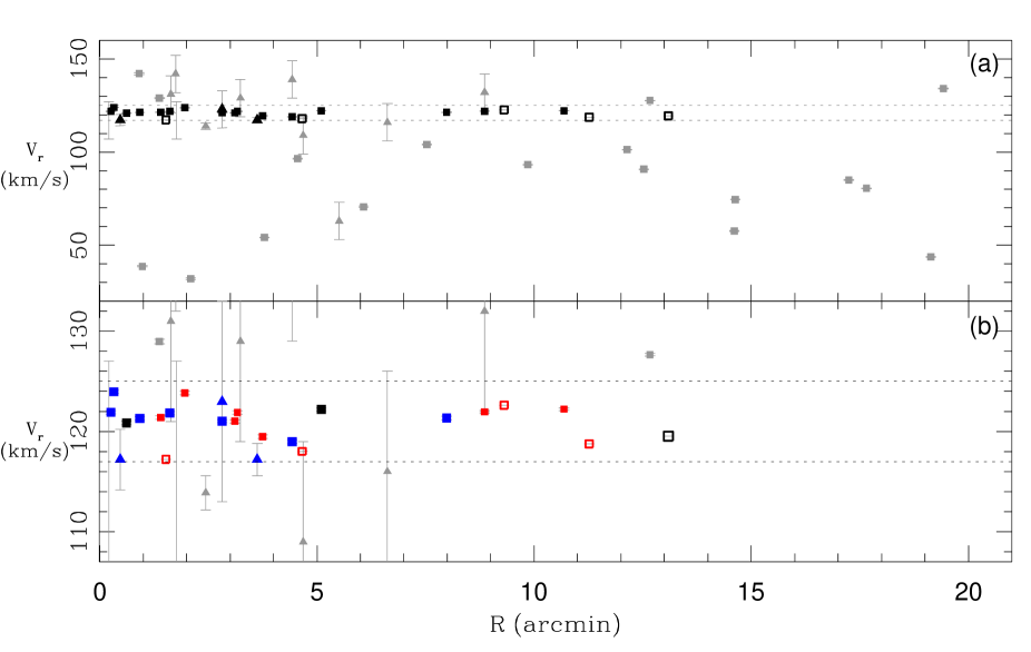
Figure 2: (a) The distribution of all new and previously measured radial velocities (with error bars) for stars in the field of Tombaugh 2 as a function of their projected distance from the cluster centre. Squares denote stars observed in this study, with filled squares denoting those observed with GIRAFFE and open squares representing those with UVES spectra. Stars selected to be RV members are shown by black symbols. Triangles denote RVs from Brown et al. (1996) and Friel et al. (2002), with darker triangles denoting members from these studies by our RV definition. (b) Same as (a) but with metallicity information for member stars shown by colour: red points are “metal-rich” ([Fe/H] $>-$0.15) and blue points are “metal-poor” ([Fe/H] $\leq-$0.15) — see the discussion in §5.

4 Abundance analysis

4.1 Atomic parameters and equivalent widths

The analysis of chemical abundances was carried out with the latest version (2005) of the program MOOG (Sneden, 1973) and using model atmospheres by Kurucz (1979). MOOG performs its analysis in local thermodynamic equilibrium (LTE). We derived equivalent widths of unblended spectral lines by using a semi-automatic SuperMongo program written by one of the authors. Repeated measurements show a typical error of about 5-10mÅ for the weakest lines because of the relatively low $S/N$ of the spectra (UVES: $\sim 20$, GIRAFFE: 60–70 ) compared to those typically used in chemical abundance studies. The line list was taken from Gratton et al. (2003) for UVES spectra, and from the VALD (Vienna Atomic Line Database; Kupka et al. 1999) database for GIRAFFE spectra. The log($gf$) parameters of these lines were redetermined by a solar-inverse analysis measuring the equivalent widths from the NOAO solar spectrum and adopting the standard solar parameters [$T_{eff}$ = 5777 K, log($g$) = 4.44, and $v_{t}$ = 0.8 km s^-1]. The solar abundances found by this analysis are reported in Table 2. For each element we give also the number of measured spectral lines. In one case (Ni I) the solar abundances for UVES and GIRAFFE spectra differ by more than 0.2 dex. The reason is that we decided to adjust the log($gf$) values only to remove the scatter affecting each line list and not to register the two line lists onto a common scale; as a result there remains a possible systematic offset for Ni I.

Table 2: Adopted solar abundances for UVES and GIRAFFE spectra.

Element	UVES	# lines	GIRAFFE	# lines
Fe I	7.48	50	7.51	40
Fe II	7.51	4	7.52	6
Na I	6.31(LTE)	2
Mg I	7.53	1
Si I	7.61	1
Ca I	6.37	2	6.55	2
Ti I	4.93	9	5.08	7
Ti II	4.96	11	5.08	3
Cr I	5.65	5	5.66	7
Cr II	5.72	2
Ni I	6.26	11	6.51	4
Ba II	2.45	2

Table 3: Sensitivity of derived abundances to the atmospheric parameters.

	$\Delta(T)$	$\Delta(\log(g))$	$\Delta(v_{t})$
Element	(per +100 K)	(per +0.2)	(per +0.2 km s-1)
Fe I	$+$0.07	$+$0.02	$-$0.07
Fe II	$-$0.07	$+$0.10	$-$0.06
Na I	$+$0.08	$-$0.04	$+$0.04
Mg I	$-$0.08	$-$0.04	$+$0.06
Si I	$-$0.02	$+$0.02	$+$0.05
Ca I	$+$0.09	$-$0.04	$-$0.09
Ti I	$+$0.15	$-$0.02	$-$0.11
Ti II	$-$0.01	$+$0.10	$+$0.12
Cr I	$+$0.13	$-$0.05	$-$0.10
Cr II	$-$0.04	$+$0.09	$-$0.10
Ni I	$-$0.08	$+$0.00	$+$0.11
Ba II	$+$0.03	$+$0.05	$-$0.15

4.2 Atmospheric parameters

Initial estimates of the atmospheric parameter $T_{\rm{eff}}$ were obtained from photometric observations using the relations from Alonso et al. (1999). We first adopted $E(B-V)$ = 0.35 (Brown et al., 1996) to correct colours for the interstellar extinction. We then adjusted the effective temperature to minimize the slope of the abundances obtained from Fe I lines with respect to the excitation potential in the curve of growth analysis. Initial guesses for the gravity, $\log{g}$ were derived from the canonical formula:

$$\log\left(\frac{g}{g_{\odot}}\right)=\log\left(\frac{M}{M_{\odot}}\right)+4\log\left(\frac{T_{\rm{eff}}}{T_{\odot}}\right)-\log\left(\frac{L}{L_{\odot}}\right)$$ (1)

In this equation the mass $M/M_{\odot}$ was derived from the comparison between the position of the star in the colour-magnitude diagram and the Padova isochrones (Girardi et al., 2000). The luminosity $L/L_{\odot}$ was derived from the absolute magnitude $M_{V}$, assuming a distance modulus of $(m-M)_{V}=15.3$ (Kubiak et al., 1992). The bolometric correction (BC) was derived from the BC-$T_{\it eff}$ relation from Alonso et al. (1999). The input $\log{g}$ values were then adjusted in order to satisfy the ionization equilibrium of Fe I and Fe II during the abundance analysis. Finally, the microturbulence velocity is given by the relation (Houdashelt, Bell & Sweigart, 2000):

$$v_{\rm t}=2.22-0.322\log g$$ (2)

We then adjusted the microturbulence velocity by minimizing the slope of the abundances obtained from Fe I lines with respect to the equivalent width in the curve of growth analysis. From the derived spectroscopic temperatures, we are able to obtain the intrinsic $(B-V)$ colours for our stars using Alonso et al. (1999). We find that for these stars that $E(B-V)\sim 0.30\pm 0.04$, in agreement with the reddening estimate for To2 by Brown et al. (1996). The final derived stellar parameters are listed in Table 1. The uncertainties in the spectroscopically determined stellar parameters are of the order of $\pm$100 K in $T_{eff}$, $\pm$0.2 in $log(g)$, and $\pm$0.2 km s^-1 in microturbolent velocity for red giant stars (see Friel et al., 2005). Table 3 lists the impact of uncertainties in the atmospheric parameters on the derived abundances for the elements considered in our analysis. Variations in parameters of the model atmospheres were obtained by changing each of the parameters one at a time for one of the analyzed stars (#179), assumed to be representative of all the stars considered in this paper.

4.3 Stellar abundances

The derived abundances from the UVES spectra are presented in Table 4. In addition to the UVES spectra, we also derive some abundances from the bright GIRAFFE spectra of cluster members (membership is described above in §3), using the same techniques described above. The derived abundances from the GIRAFFE spectra are listed in Tables 5 and 6, together with their uncertainties.

The Na abundance was obtained from the spectral lines at 5662-8 and 6154-60 Å. These features are well known to be affected by NLTE effects. For this reason we applied an NLTE correction from Gratton et al. (1999) to the output LTE abundances (see Table 4).

Table 4: Measured Abundances for UVES stars.

ID	El	(X)	ELMeas	EL⊙	#	[El/X]
158	Fe I	(H)	7.42$\pm$0.04	7.48	31	$-$0.06$\pm$0.04
158	Fe II	(H)	7.45$\pm$0.14	7.51	3	$-$0.06$\pm$0.14
158	Na I(568)	(Fe)	6.51$\pm$0.07	6.31	2	$+$0.26$\pm$0.08L
						$+$0.31$\pm$0.08N
158	Na I(616)	(Fe)	6.17	6.31	1	$-$0.08L
						$+$0.07N
158	Mg I	(Fe)	7.25	7.53	1	$-$0.22
158	Si I	(Fe)	7.72$\pm$0.10	7.61	2	$+$0.17$\pm$0.11
158	Ca II	(Fe)	6.34$\pm$0.07	6.37	5	$+$0.03$\pm$0.08
158	Ti I	(Fe)	5.07$\pm$0.07	4.93	7	$+$0.20$\pm$0.08
158	Ti II	(Fe)	4.93$\pm$0.10	4.96	2	$+$0.03$\pm$0.11
158	Cr I	(Fe)	5.60$\pm$0.13	5.65	5	$+$0.01$\pm$0.14
158	Cr II	(Fe)	5.64	5.72	1	$-$0.02
158	Ni I	(Fe)	6.21$\pm$0.08	6.26	7	$+$0.01$\pm$0.09
158	Ba I	(Fe)	1.98$\pm$0.08	2.45	2	$-$0.41$\pm$0.09
158	$\alpha$	(Fe)				$+$0.04$\pm$0.08
162	Fe I	(H)	7.44$\pm$0.04	7.48	35	$-$0.04$\pm$0.04
162	Fe II	(H)	7.47$\pm$0.10	7.51	4	$-$0.04$\pm$0.10
162	Na I(568)	(Fe)	6.87$\pm$0.09	6.31	2	$+$0.60$\pm$0.10L
						$+$0.65$\pm$0.10N
162	Na I(616)	(Fe)	6.35	6.31	1	$+$0.08L
						$+$0.23N
162	Mg I	(Fe)	7.55	7.53	1	$+$0.06
162	Si I	(Fe)	7.72$\pm$0.08	7.61	2	$+$0.15$\pm$0.09
162	Ca II	(Fe)	6.26$\pm$0.09	6.37	5	$-$0.07$\pm$0.10
162	Ti I	(Fe)	4.99$\pm$0.09	4.93	8	$+$0.10$\pm$0.10
162	Ti II	(Fe)	5.15$\pm$0.16	4.96	2	$+$0.23$\pm$0.16
162	Cr I	(Fe)	5.80$\pm$0.13	5.65	3	$+$0.19$\pm$0.14
162	Cr II	(Fe)	5.78$\pm$0.06	5.72	2	$+$0.10$\pm$0.07
162	Ni I	(Fe)	6.29$\pm$0.07	6.26	7	$+$0.07$\pm$0.08
162	Ba I	(Fe)	2.10$\pm$0.10	2.45	2	$-$0.31$\pm$0.11
162	$\alpha$	(Fe)				$+$0.09$\pm$0.05
164	Fe I	(H)	7.39$\pm$0.03	7.48	49	$-$0.09$\pm$0.03
164	Fe II	(H)	7.42$\pm$0.10	7.51	3	$-$0.09$\pm$0.10
164	Na I(568)	(Fe)	6.36$\pm$0.07	6.31	2	$+$0.14$\pm$0.07L
						$+$0.19$\pm$0.08N
164	Na I(616)	(Fe)	6.23	6.31	1	$+$0.01L
						$+$0.16N
164	Mg I	(Fe)	7.30	7.53	1	$-$0.14
164	Si I	(Fe)	7.62$\pm$0.05	7.61	2	$+$0.10$\pm$0.06
164	Ca II	(Fe)	6.30$\pm$0.05	6.37	9	$+$0.02$\pm$0.06
164	Ti I	(Fe)	5.14$\pm$0.04	4.93	11	$+$0.30$\pm$0.05
164	Ti II	(Fe)	5.23$\pm$0.08	4.96	2	$+$0.36$\pm$0.08
164	Cr I	(Fe)	5.77$\pm$0.11	5.65	5	$+$0.21$\pm$0.11
164	Cr II	(Fe)	5.89$\pm$0.07	5.72	2	$+$0.26$\pm$0.08
164	Ni I	(Fe)	6.25$\pm$0.06	6.26	11	$+$0.08$\pm$0.07
164	Ba I	(Fe)	2.52$\pm$0.01	2.45	2	$+$0.16$\pm$0.02
164	$\alpha$	(Fe)				$+$0.13$\pm$0.10
165	Fe I	(H)	7.41$\pm$0.05	7.48	26	$-$0.07$\pm$0.05
165	Fe II	(H)	7.44$\pm$0.09	7.51	4	$-$0.07$\pm$0.09
165	Na I(568)	(Fe)	6.36$\pm$0.01	6.31	2	$+$0.12$\pm$0.05L
						$+$0.17$\pm$0.05N
165	Na I(616)	(Fe)	6.43	6.31	1	$+$0.19L
						$+$0.34N
165	Mg I	(Fe)	7.18	7.53	1	$-$0.28
165	Si I	(Fe)	7.72$\pm$0.18	7.61	2	$+$0.18$\pm$0.19
165	Ca II	(Fe)	6.30$\pm$0.07	6.37	8	$+$0.00$\pm$0.09
165	Ti I	(Fe)	5.18$\pm$0.11	4.93	7	$+$0.32$\pm$0.12
165	Ti II	(Fe)	5.01$\pm$0.64	4.96	2	$+$0.12$\pm$0.64
165	Cr I	(Fe)	5.77$\pm$0.14	5.65	5	$+$0.19$\pm$0.15
165	Cr II	(Fe)		5.72	0
165	Ni I	(Fe)	6.37$\pm$0.08	6.26	4	$+$0.18$\pm$0.09
165	Ba I	(Fe)	2.40$\pm$0.16	2.45	2	$+$0.02$\pm$0.17
165	$\alpha$	(Fe)				$-$0.07$\pm$0.11

^N NLTE solution

^L LTE solution

Table 5: Measured Abundances for GIRAFFE stars.

ID	El	(X)	ELMeas	EL⊙	#	[El/X]
63	Fe I	(H)	7.32$\pm$0.05	7.51	34	$-$0.19$\pm$0.05
63	Fe II	(H)	7.34	7.52	1	$-$0.18
63	Ti I	(Fe)	5.09$\pm$0.15	5.08	6	$+$0.20$\pm$0.16
63	Ti II	(Fe)	5.08$\pm$0.15	5.08	3	$+$0.19$\pm$0.16
63	Cr I	(Fe)	5.17$\pm$0.26	5.66	6	$-$0.30$\pm$0.26
63	Ni I	(Fe)	6.12$\pm$0.19	6.51	4	$-$0.20$\pm$0.20
98	Fe I	(H)	7.45$\pm$0.05	7.51	27	$-$0.06$\pm$0.05
98	Fe II	(H)	7.45$\pm$0.08	7.52	3	$-$0.07$\pm$0.08
98	Ti I	(Fe)	5.15$\pm$0.13	5.08	6	$+$0.13$\pm$0.14
98	Ti II	(Fe)	5.00$\pm$0.13	5.08	3	$-$0.02$\pm$0.14
98	Cr I	(Fe)	5.16$\pm$0.18	5.66	4	$-$0.44$\pm$0.19
98	Ni I	(Fe)	5.89$\pm$0.17	6.51	3	$-$0.56$\pm$0.18
102	Fe I	(H)	7.25$\pm$0.06	7.51	19	$-$0.26$\pm$0.06
102	Fe II	(H)	7.29$\pm$0.01	7.52	2	$-$0.23$\pm$0.01
102	Ti I	(Fe)	5.20$\pm$0.09	5.08	5	$+$0.38$\pm$0.11
102	Ti II	(Fe)	5.29$\pm$0.15	5.08	2	$+$0.47$\pm$0.16
102	Cr I	(Fe)	5.21$\pm$0.16	5.66	3	$-$0.19$\pm$0.17
102	Ni I	(Fe)	6.27$\pm$0.17	6.51	2	$+$0.02$\pm$0.18
124	Fe I	(H)	7.47$\pm$0.04	7.51	25	$-$0.04$\pm$0.04
124	Fe II	(H)	7.47$\pm$0.17	7.52	2	$-$0.05$\pm$0.17
124	Ti I	(Fe)	5.35$\pm$0.13	5.08	5	$+$0.31$\pm$0.14
124	Ti II	(Fe)	5.45$\pm$0.29	5.08	3	$+$0.41$\pm$0.29
124	Cr I	(Fe)	5.46$\pm$0.06	5.66	3	$-$0.16$\pm$0.07
124	Ni I	(Fe)	6.18	6.51	1	$-$0.29
127	Fe I	(H)	7.16$\pm$0.06	7.51	27	$-$0.35$\pm$0.06
127	Fe II	(H)	7.17$\pm$0.02	7.52	2	$-$0.35$\pm$0.02
127	Ti I	(Fe)	4.97$\pm$0.13	5.08	7	$+$0.24$\pm$0.14
127	Ti II	(Fe)	5.31$\pm$0.50	5.08	2	$+$0.58$\pm$0.50
127	Cr I	(Fe)	4.74$\pm$0.19	5.66	4	$-$0.57$\pm$0.20
127	Ni I	(Fe)	6.19$\pm$0.18	6.51	2	$+$0.03$\pm$0.19
135	Fe I	(H)	7.43$\pm$0.06	7.51	27	$-$0.08$\pm$0.06
135	Fe II	(H)	7.44$\pm$0.08	7.52	2	$-$0.08$\pm$0.85
135	Ti I	(Fe)	5.17$\pm$0.15	5.08	6	$+$0.17$\pm$0.16
135	Ti II	(Fe)	5.22$\pm$0.11	5.08	3	$+$0.22$\pm$0.12
135	Cr I	(Fe)	5.00$\pm$0.25	5.66	5	$-$0.58$\pm$0.26
135	Ni I	(Fe)	6.28$\pm$0.10	6.51	2	$-$0.15$\pm$0.12
140	Fe I	(H)	7.50$\pm$0.07	7.51	21	$-$0.01$\pm$0.07
140	Fe II	(H)	7.50$\pm$0.16	7.52	2	$-$0.02$\pm$0.16
140	Ti I	(Fe)	5.08$\pm$0.06	5.08	5	$+$0.01$\pm$0.09
140	Ti II	(Fe)	4.98$\pm$0.49	5.08	2	$-$0.09$\pm$0.49
140	Cr I	(Fe)	5.07$\pm$0.25	5.66	4	$-$0.58$\pm$0.26
140	Ni I	(Fe)	6.45$\pm$0.11	6.51	2	$-$0.05$\pm$0.13
177	Fe I	(H)	7.08$\pm$0.05	7.51	20	$-$0.43$\pm$0.05
177	Fe II	(H)	7.09$\pm$0.12	7.52	3	$-$0.43$\pm$0.12
177	Ti I	(Fe)	5.00$\pm$0.18	5.08	4	$+$0.35$\pm$0.19
177	Ti II	(Fe)	5.19$\pm$0.11	5.08	2	$+$0.54$\pm$0.12
177	Cr I	(Fe)	5.05$\pm$0.20	5.66	5	$-$0.18$\pm$0.21
177	Ni I	(Fe)	5.79$\pm$0.28	6.51	2	$-$0.29$\pm$0.28
179	Fe I	(H)	7.46$\pm$0.04	7.51	22	$-$0.05$\pm$0.04
179	Fe II	(H)	7.46$\pm$0.25	7.52	2	$-$0.06$\pm$0.25
179	Ti I	(Fe)	5.16$\pm$0.19	5.08	5	$+$0.23$\pm$0.19
179	Ti II	(Fe)	5.16$\pm$0.36	5.08	2	$+$0.13$\pm$0.36
179	Cr I	(Fe)	4.59	5.66	1	$-$1.02
179	Ni I	(Fe)		6.51	0
182	Fe I	(H)	7.47$\pm$0.07	7.51	20	$-$0.04$\pm$0.07
182	Fe II	(H)	7.48$\pm$0.39	7.52	2	$-$0.04$\pm$0.39
182	Ti I	(Fe)	5.25$\pm$0.17	5.08	5	$+$0.21$\pm$0.18
182	Ti II	(Fe)	4.94$\pm$0.12	5.08	3	$-$0.10$\pm$0.14
182	Cr I	(Fe)	5.27$\pm$0.25	5.66	4	$-$0.35$\pm$0.26
182	Ni I	(Fe)	6.39	6.51	1	$-$0.08

Table 6: Measured Abundances for GIRAFFE stars (Cont).

ID	El	(X)	ELMeas	EL⊙	#	[El/X]
191	Fe I	(H)	7.26$\pm$0.06	7.51	19	$-$0.25$\pm$0.06
191	Fe II	(H)	7.23$\pm$0.48	7.52	3	$-$0.29$\pm$0.48
191	Ti I	(Fe)	5.21$\pm$0.18	5.08	4	$+$0.38$\pm$0.19
191	Ti II	(Fe)	4.99$\pm$0.26	5.08	2	$+$0.16$\pm$0.27
191	Cr I	(Fe)	5.29$\pm$0.07	5.66	3	$-$0.12$\pm$0.09
191	Ni I	(Fe)	6.35$\pm$0.11	6.51	2	$+$0.09$\pm$0.12
196	Fe I	(H)	7.23$\pm$0.06	7.51	23	$-$0.28$\pm$0.06
196	Fe II	(H)	7.26$\pm$0.08	7.52	3	$-$0.26$\pm$0.08
196	Ti I	(Fe)	5.30$\pm$0.17	5.08	3	$+$0.50$\pm$0.18
196	Ti II	(Fe)	4.93$\pm$0.16	5.08	3	$+$0.13$\pm$0.17
196	Cr I	(Fe)	5.03$\pm$0.25	5.66	4	$-$0.35$\pm$0.26
196	Ni I	(Fe)	6.31$\pm$0.36	6.51	4	$+$0.08$\pm$0.36
199	Fe I	(H)	7.30$\pm$0.04	7.51	20	$-$0.21$\pm$0.04
199	Fe II	(H)	7.31$\pm$0.42	7.52	3	$-$0.21$\pm$0.42
199	Ti I	(Fe)	4.99$\pm$0.15	5.08	5	$+$0.12$\pm$0.15
199	Ti II	(Fe)	5.23$\pm$0.06	5.08	2	$+$0.36$\pm$0.07
199	Cr I	(Fe)	5.33$\pm$0.15	5.66	4	$-$0.12$\pm$0.15
199	Ni I	(Fe)	6.50	6.51	1	$+$0.20
231	Fe I	(H)	7.42$\pm$0.05	7.51	23	$-$0.09$\pm$0.05
231	Fe II	(H)	7.43$\pm$0.11	7.52	2	$-$0.09$\pm$0.11
231	Ti I	(Fe)	5.46$\pm$0.12	5.08	5	$+$0.47$\pm$0.13
231	Ti II	(Fe)	5.11$\pm$0.10	5.08	2	$+$0.12$\pm$0.11
231	Cr I	(Fe)	5.32$\pm$0.11	5.66	5	$-$0.25$\pm$0.12
231	Ni I	(Fe)	6.35$\pm$0.10	6.51	3	$-$0.07$\pm$0.11

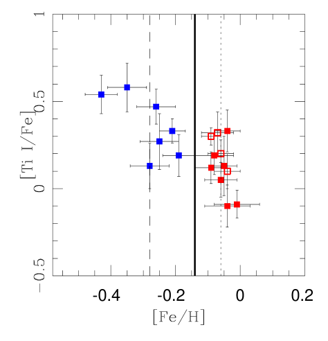
Figure 3: Plot of the derived [Fe/H] vs. [Ti I/Fe] for the “members” from our analysis. Red points denote “metal-rich” and blue points are “metal-poor”, same as Fig 1b.. The dotted line denotes the “mean” [Fe/H] value for the MR sample ($-$0.06), the dashed line for the MP sample ($-$0.28), and the solid line for the combined sample ($-$0.14) for the cluster if all stars are members.

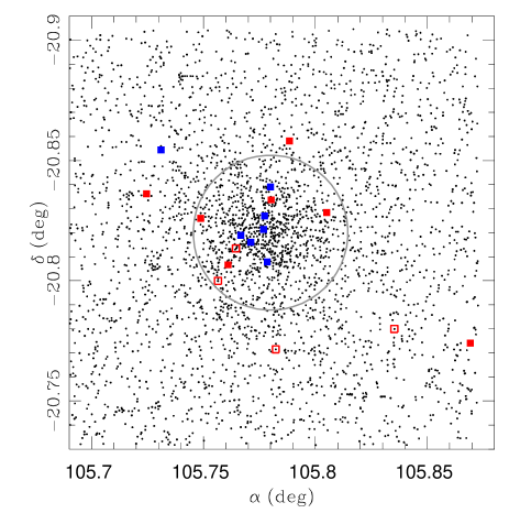
Figure 4: Spatial distribution of To2 stars from Phelps et al. (1994) photometry. Marked stars are “members” from our analysis, with red points denoting “metal-rich” and blue points “metal-poor.” Open boxes denote the UVES stars. The gray circle denotes a typical open clusters tidal radius of 10 pc (Piskunov et al., 2008) scaled to the distance of To2. However as To2 is in the outer disc and older, and therefore presumibly more massive than the typical open cluster, the shown tidal radius should be taken as a lower limit to the extent of the cluster.

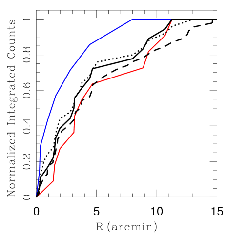
Figure 5: Integrated counts of stars with RVs with 15 arcmin of the cluster centre. The dotted line represents all stars with RVs (Brown et al. 1996; Friel et al. 2000; ours), while the dashed line is all member stars. The black solid line represents all of the members found in our study (excluding the stars of Brown et al., 1996; Friel et al., 2002). Finally, the red line show the distribution of our “metal-rich” members and the blue line our “metal-poor” members.

5 Chemical Abundances and Cluster Kinematics Revisited

Our abundance analysis of To2 finds a surprising spread in [Fe/H] for stars selected as members based on their RVs. In Figure 3, we show the distribution of [Ti I/Fe] versus [Fe/H] abundance ratios, which shows a strong overall correlation but also an apparent divide at [Fe/H] $=-0.15$ dex. Even if the division into two populations is not real and the metallicity variation is more continuous, dividing the sample into two parts still provides a handy way to explore properties as a function of metallicity. To investigate this distribution further, we select two sub-samples by using the apparent divide at [Fe/H] $=-0.15$ dex and denote these as the “metal-rich” group (MR; [Fe/H] $>-0.15$ dex; red points) and the “metal-poor” group (MP; [Fe/H] $\leq-0.15$ dex; blue points).

The spatial distribution of the two sub-samples is shown in Figure 4 as well as in Figure 2b. We find that the MP group is more centrally concentrated, as shown by the integrated counts in Figure 5, though both groups could reasonably belong to the cluster. Even if we account for the selection effect of how stars were targeted for spectroscopy (the dotted line in Fig. 5) the MP stars still show a significant central concentration. The summary of kinematics and abundances for these sub-groups are listed in Table 8, showing [Fe/H], [Ti I/Fe], [Cr/Fe], [Ni/Fe], as well as the mean velocity ($\langle V_{r}\rangle$) and velocity dispersion ($\sigma_{int}$). As may be seen from Table 8, the kinematical properties of the two samples are basically indistinguishable, so that kinematics do little to help understand the origin of the metallicity spread/differences among the RV-members. Figure 6 shows the distribution of MP and MR stars in the colour-magnitude diagram (CMD) for To2, using the photometry from Phelps et al. (1994) and demonstrates that both populations also lie in areas of the CMD expected for member stars.

5.1 Stellar abundance reliability

Given that an abundance spread in an open cluster is an unprecedented find, one of the first points to explore is whether our derived metallicities, and the implied spread in chemistry for stars with the RV of To2, could be artificially induced by errors in our analysis. Two possible sources of errors can mimic a spread in metallicity:

1. Differential reddening could alter colours an unknown amount, thereby affecting the derived temperature, producing a spread in metallicity. However, for differential reddening to explain the observed abundance spread across both samples (0.4 dex) would require reddening differences of $>0.2$ $E(B-V)$, which is not possible given the observed CMD and our spectral analysis. Moreover, Figure 4 shows that the MP and MR stars are mixed in their spatial distribution. In any case for our study the temperatures derived from photometry were used only as first guess in an iterative procedure that allowed us to find the atmospheric parameters directly from spectral data, and this spectral analysis reveals a reddening spread of only $\delta E(B-V)\sim 0.04$ (§4.2). As a result, we can exclude differential reddening as a possible source for the observed metallicity spread in To2.

2. Random errors in temperature can introduce random errors in the derived metallicity. However, such errors are difficult to estimate for our To2 data both because of the relatively small numbers of stars in our sample, and because of the suspected intrinsic metallicity spread of our stars. The determination of the random error from $T_{eff}$ and that of the abundance determinations are coupled, so that if the metallicity spread is true it would lead to an overestimation of the random error due to the $T_{eff}$ uncertainty. To get around this problem, we therefore compare our derived $T_{eff}$ uncertainty to another analyzed cluster without an abundance spread to evaluate the reliability of our abundance determinations. We estimated the whole error (the error due to the equivalent width measurement and given by MOOG + the error due to the $T_{eff}$ uncertainty) referring to a study on the globular cluster M4 (Marino et al., in preparation). Some of the authors of the present study of To2 also derived chemical abundances for a large statistic sample of stars in M4 using the same method adopted here on spectra having the same wavelength range and comparable $S/N$. Assuming a homogenous composition for the stars in M4 (an assumption usually true for most of the elements in a globular cluster with the exception of the light ones) a dispersion ($\sigma$) was found in the iron content of 0.06 dex for GIRAFFE data and of 0.05 dex for UVES ones. These observed dispersions can be considered as a good estimate of the whole random error to be used in our study of To2. In Table 7 we report the dispersion for all the elements considered in this study as derived from the M4 data. Given that our measured uncertainties on the abundance determination are consistent between the M4 and To2 analysis, we find that errors in the determination of $T_{eff}$ cannot be the source of the observed abundance spread.

We find that random observational errors cannot explain the mean difference of 0.22 dex (see Table 8) in metallicity observed in To2 between the metal rich and the metal poor group. Additionally, since systematic errors introduced by the method affect all the results in the same way, these also cannot explain the observed abundance spread. At this point we conclude that the observed spread in metallicity in our sample is real.

Table 7: Measured Abundance Ratios for UVES stars.

	$\sigma$ from M4	$\sigma$ from M4
Element	(GIRAFFE)	(UVES)
error (FeI)	0.06	0.05
error (FeII)	0.06	0.05
error (TiI)	0.06	0.04
error (TiII)	0.10	0.06
error (CrI)	0.10	0.05
error (CrII)		0.08
error (Ni)	0.07	0.03
error (SiI)		0.05
error (CaI)		0.03
error (BaII)		0.03

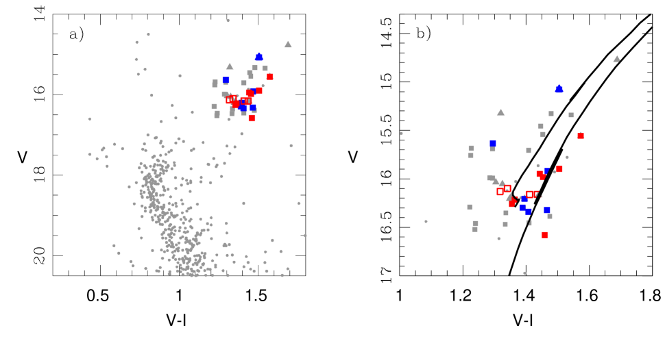
Figure 6: (a) Colour-magnitude diagram for stars within a 2’ radius of To2 from Phelps et al. (1994), plus all stars with current and previous RV determinations. Squares denote observations with VLT/FLAMES+GIRAFFE, open squares with VLT/FLAMES+UVES, and triangles are previous observations (Brown et al., 1996; Friel et al., 2002). Red and blue symbols are members based on their RV. All symbols same as Figure 1. (b) RGB and red clump from (a) with a Padova isochrone of $Z=0.0164$, age = 2.0 Gyr, $d=8.4$ kpc, and $E(B-V$) = 0.25 overplotted.

.

5.2 Comparison to previous findings

Brown et al. (1996) conducted a high resolution (R $\sim$ 34,000) study of To2 with the CTIO 4-m telescope and found [Fe/H] = $-$0.4 $\pm$ 0.25 for $E(B-V)=0.4$ or [Fe/H] = $-$0.5 $\pm$ 0.25 for $E(B-V)=0.3$ based on three stars, with [Fe/H] = $-$0.2, $-$0.4, and $-$0.57. The Brown et al. (1996) abundance analysis showed that To2 has a reddening of $E(B-V$) = 0.3–0.4, which is consistent with our spectroscopically measured reddening. Unfortunately we do not have stars in common with the Brown et al. (1996) sample for a direct comparison of our metallicity derivations, but the metallicities of their three stars are within the range of our derived [Fe/H], accounting for the errors, for To2 members. However, the more metal-rich of the three Brown et al. stars is ruled out as a cluster member based on our radial velocity criterion.

Another study of cluster metallicities including To2 was conducted by Friel et al. (2002) using the CTIO 4-m/ARGUS, which yielded a much lower resolution ($R\sim 1300$) than either our study or that of Brown et al. (1996), and with metallicities determined from spectral indices. Friel et al. (2002) found [Fe/H] = $-$0.44 $\pm$ 0.09 for To2 from a sample of 12 member stars, and with the individual measurements ranging from $-$0.28 to $-$0.65. Friel et al. (2002) found nearly identical metallicities for the two stars in common with Brown et al. (1996). We observed three other Friel et al. (2002) stars with the GIRAFFE spectrograph but find poor agreement with the previous low-resolution results in 2 of the 3 stars, as shown in Table 9, where ID is from Phelps et al. (1994) and ID2 is from Kubiak et al. (1992). It should be pointed out that sometimes high-resolution studies to find slightly higher metallicities when compared with low-resolution studies based on spectral indices (e.g., in the high resolution study of Berkeley 17, Friel et al. 2005 find [Fe/H] = $-0.10\pm 0.09$ as compared to [Fe/H] = $-0.33\pm 0.13$ from the low-resolution spectroscopy of Friel et al. 2002).

Table 8: GIRAFFE Spectra Radial Velocity and Abundance “Sub-Populations”

Sample	# Stars	[Fe/H]	[Ti I/Fe]	[Cr/Fe]	[Ni/Fe]	$\langle V_{r}\rangle$	$\sigma_{int}$
						(km s-1)	(km s-1)
Metal-rich (UVES only)	4	$-$0.07$\pm$0.01	$+$0.23$\pm$0.06	$+$0.15$\pm$0.05	$+$0.08$\pm$0.04	119.2$\pm$1.0	2.1$\pm$0.7
Metal-rich (GIRAFFE only)	7	$-$0.05$\pm$0.02	$+$0.14$\pm$0.05	$-$0.48$\pm$0.12	$-$0.20$\pm$0.09	121.7$\pm$0.5	1.2$\pm$0.3
Metal-rich (UVES+GIRAFFE)	11	$-$0.06$\pm$0.01	$+$0.23$\pm$0.03	$-$0.25$\pm$0.07	$-$0.05$\pm$0.05	120.8$\pm$0.6	2.0$\pm$0.4
Metal-poor (GIRAFFE)	7	$-$0.28$\pm$0.03	$+$0.32$\pm$0.06	$-$0.26$\pm$0.06	$-$0.01$\pm$0.07	121.5$\pm$0.5	1.4$\pm$0.4
All RV Members	18	$-$0.14$\pm$0.03	$+$0.24$\pm$0.03			121.0$\pm$0.4	1.8$\pm$0.3

Table 9: Comparison of Friel et al. (2002) and GIRAFFE Data

ID	ID2	$V_{r,GIRAFFE}$	$V_{r,Friel}$	$\Delta$ $V_{r}$	[Fe/H]GIRAFFE	[Fe/H]Friel	$\Delta$[Fe/H]
		(km s-1)	(km s-1)	(km s-1)
63	20	120.96 $\pm$ 0.16	123 $\pm$ 10	2	$-$0.19$\pm$0.05	$-$0.40$\pm$0.10	0.21
98	28	121.71 $\pm$ 0.18	132 $\pm$ 10	10	$-$0.06$\pm$0.05	$-$0.48$\pm$0.22	0.42
177	61	118.74 $\pm$ 0.16	139 $\pm$ 10	20	$-$0.43$\pm$0.05	$-$0.39$\pm$0.31	0.04

5.3 Revised reddening and distance

From the stars that have been selected as members, we have determined the cluster mean metal abundance for the MP and MR sub-samples (see Table 8). We have generated isochrones for the exact metallicity of each cluster sample, transforming the mean [Fe/H] into $Z$, using Padova models and following Carraro et al. (1999). The corresponding by-eye fit isochrone is then superposed on the CMD, with stars of the other abundance sample removed, and fitted to the data distribution (Figure 6). In Figure 7, we match Padova isochrones to the ($V$, $V-I$) CMDs from Phelps et al. (1994). We show these matches with stars from the inner 2 arcmin of the clusters plus RV members selected from the MP (Figure 7a) and MR (Figure 7b) samples. Estimates of the basic parameters (age, distance and reddening) are derived from comparison to the Padova isochrones. Our best fit for both samples is: age = 2.0 Gyr, $E(B-V)=0.3$, and $(m-M)_{0}=14.5$ or $d=7.9$ kpc and $R_{GC}=14.2$ kpc. Additionally, the spectroscopy yields a reddening in the range 0.3–0.35 which is consistent with isochrone fitting to both samples; however, we find the value of $E(B-V$) = 0.40 found by Kubiak et al. (1992) cannot provide a good fit to the ($V$, $V-I$) CMDs using the Phelps et al. (1994) photometry. Our spectroscopically determined reddening is also consistent with a newer near-infrared study (Kyeong & Byun, 2000) who found $E(B-V$) = 0.24 $\pm$ 0.12.

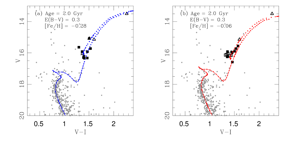
Figure 7: CMDs for To2 showing best fit Padova isochrones. (a) Padova $Z=0.00955$ ([Fe/H] = $-$0.28) isochrone fit is shown with MP members and other RV members without metallicity determinations. (b) Padova $Z=0.01665$ ([Fe/H] = $-$0.06) isochrone fit is shown with MR members and other RV members without metallicity determinations.

6 Discussion

While this study was intended to verify or refute the connection of To2 with the Monoceros stream/Galactic anticenter stellar structure (GASS), our work has produced more questions than answers. The observed spread in To2 metallicity and $\alpha$-abundances was not expected and cannot be simply explained. To date, no other open cluster is known to have a metallicity spread, and it is difficult to understand how a low-mass open cluster might have been able to retain gas after an initial starburst to self-enrich. Next, we review our findings and possible scenarios that could explain the data

6.1 Are both populations part of Tombaugh 2?

First, we ask the question of whether both the MP and MR groups among the To2 RV members are likely to be truly part of the cluster, and then investigate the likelihood that either population is simply contamination of the RV member sample.

6.1.1 Is the metal poor population part of Tombaugh 2?

To2 has been proposed to be part of the putative GASS cluster system (Frinchaboy et al., 2004; Martin et al., 2004a), and the MP population is similar, though slightly more metal rich than, other studied Monoceros candidate clusters such as Saurer 1 (Frinchaboy & Phelps, 2002; Carraro & Baume, 2003; Carraro et al., 2004), Berkeley 29 (Carraro et al., 2004; Yong et al., 2005), and Palomar 1 (Rosenberg et al., 1998; Sarajedini et al., 2007). These clusters all have ages of approximately 4–6 Gyr, metallicities between $-$0.7 and $-$0.4 dex, and are all $\alpha$–enhanced. Our To2 MP group is younger though similarly moderately metal poor ([Fe/H] $\sim$ $-$0.3) and also $\alpha$–enhanced. This is at least circumstantial evidence that the MP group might be the more likely member population. This subgroup also has a metallicity roughly consistent with previous metallicity determinations for To2 by Brown et al. (1996) and Friel et al. (2002) — though it is not impossible that these other researchers could have also been hit with a spate of bad luck in terms of misleading target selection.

On the other hand, it must also be admitted that the MP group both exhibits more scatter in terms of metallicity properties than the MR population and has a smaller number of members — though this number increases when we account for the additional “MP” members found in the Brown et al. (1996) and Friel et al. (2002) samples that are not part of our sample. Perhaps the strongest support for the supposition that the MP group is a “real” part of the cluster comes from the fact that the MP group is strongly centrally concentrated (Figs. 4 and 5) and that it has a marginally smaller velocity dispersion than the MR group, as shown in Table 8.

6.1.2 Is the metal rich population part of Tombaugh 2?

The MR population is indeed less centrally concentrated that the MP population, and in fact has a distribution function not unlike our spectroscopic sampling function, as shown in Figure 4 and 5. Given the small number statistics overall, it may not be impossible for us to have been successful at achieving a uniform “success” fraction (i.e. in identifying RV members) over the radial range sampled, even by chance. Indeed, the overall distribution of RV members very closely tracks the sampling function. Though Figure 4 clearly shows a tighter MP distribution than MR population, it is not inconceivable for there to exist a metallicity gradient in the system to yield a differential radial distribution — on the other hand, the one needed (i.e. more metal poor towards the centre) is quite unusual and not seen elsewhere.

On the other hand, the MR group has more members and is more tightly clumped in [Fe/H]. Given the tight RV distribution, chemical properties, and sheer numbers it seems difficult to believe that the MR population is not some coherent Simple Stellar Population (SSP), whether part of the cluster or a “contaminant.” We show below that this population is quite unlike that of the disc field star population (which is not an SSP).

If the true To2 stars are those in the MR group (and excluding the MP group) then To2 is less consistent with being part of the putative GASS cluster system, as it would be inconsistent with the observed metallicity distribution of Monoceros (Crane et al 2003; Sbordone et al 2005; de Jong et al. 2007). In this case, To2 would be the most distant metal-rich Milky Way disk open cluster found to date. It seems unlikely that a 2 Gyr old cluster with near solar [Fe/H] could have formed “normally” in the outer disc, given the observed, more depleted chemistry of the surrounding disc stars (e.g., Carney et al., 2005; Yong et al., 2006); this would suggest that the cluster must have formed elsewhere (e.g., in a dwarf galaxy) and been deposited in the outer disc. This is not out of line with current CDM models for the formation of Milky Way-like galaxies, which suggest that discs form from the outside via continued merging (e.g., Abadi et al 2003). Stars as metal rich as our MR group are indeed found in paradigm accretion events, like the Sagittarius dwarf (e.g., Smecker-Hane & McWilliam 2002, Monaco et al. 2005, Chou et al. 2007).

6.1.3 Can either population simply be contamination?

If we believe that only one of the two metallicity populations is truly part of To2, then the other population must be a contaminant of some kind. Here we address how likely it is that either population may be part of the Galactic disc.

We have already seen (§3) that the predicted contamination rate of normal disc stars into our RV membership range based on the Besancon model (see §3) is already smaller (by factor of 10²) than either our MP or MR samples — thus, it seems very unlikely that either population can be a statistical, “fluke” superposition of a large number of disc stars with just the right RV. From Poisson statistics, the chances that we would get 7 (e.g., MP) or 11 (e.g., MR) stars as contaminants when the models predict 0.02 stars is $1.1\times 10^{-5}$ % and $2.3\times 10^{-11}$ %, respectively. And this ignores the fact that other studies have identified additional stars in the To2 that we would categorize as “MP.”

Based on the radial distribution of members, the MP population seems more likely to be truly part of the cluster. This could then imply that the MR group is a contaminant population. However, stars this metal rich (nearly solar metallicity) at $R_{gc}\geq 15$ kpc are not consistent with the measured metallicities of red giants in the outer disc (Carney et al., 2005) as well as outer disc Cepheid stars (Yong et al., 2006), which both suggest that the median disc metallicity at this Galactocentric distance should be [Fe/H] $\sim$ -0.4. These studies of outer disc tracers find no stars as metal rich as our MR group, even for the younger Cepheid populations.

This then might suggest that the MP group could be a contaminating field population, since the chemistry of this group is more in line with that of the Carney et al. (2005) and Yong et al. (2006) stars in the outer disc. In turn, this implies that the tight radial concentration of the MP stars is a statistical anomaly. However Monte Carlo simulations show that the probability for a random disc population to achieve the observed level of concentration, taking into account our sampling function, is 0.1%. It also implies that previous spectroscopic studies had similarly “bad luck” in picking targets to represent To2.

6.2 Does Tombaugh 2 really have a metallicity spread?

The cumulative evidence for To2 — the nearly identical velocities and velocity dispersions of the stars when divided into MP and MR groups, the positions of the stars in the CMD, the unlikeliness that these stars are field contamination, etc. — suggests that all of the RV “members” in our To2 spectroscopic sample could truly be members of the system. If all RV “members” are indeed members of To2 then we are finding evidence for a significant metallicity spread within To2. That we also seem to find a similar bifurcation of [Ti I/Fe] with [Fe/H], rather than a scatter-diagram in Figure 3 is further evidence of a possible coherent chemical enrichment history. It is also possible, based on an apparent “break” in both [Fe/H] and [Ti I/Fe], that the To2 chemical and age distribution suggests the possibility that there may be two populations rather than a “trend.”

If these populations of varying chemistry do belong to To2, what formation scenarios could create such a unique open cluster?

6.2.1 Is To2 actually two “very close” clusters?

What is the possibility that two clusters with the same RV lie at nearly the same distance and have nearly the same metallicity and could also be aligned along the same line of sight? Though such a configuration could produce the observed results in the To2 field, and even account for the apparent “bimodal” behavior of the chemical distribution, it seems extremely unlikely given the small number of clusters (less than 20) known this far from the Galactic centre. It is the case that a superposition of clusters would increase the “discoverability” of this distant “double cluster”, but the individual clusters would have to be very close together along the line of sight given that a significant broadening of the main sequence is not seen in the available photometry. However new higher quality photometry would be needed to fully test this case (as was done with the Hubble Space Telescope in the case of NGC 2808; Piotto et al., 2007).

There are a few cases of overlapping clusters, with the most-well studied overlapping pair being NGC 1750 and NGC 1758, with ages of 200 $\pm$ 50 and 400 $\pm$ 100 Myr respectively (Galadí-Enríquez et al., 1998b). For NGC 1750 and NGC 1758 proper motions were required to be able to separate the two clusters separated by $\sim 130$ pc along the line of sight (Galadí-Enríquez et al., 1998b), but with little noticeable differences seen in the overlapping CMD sequences (Galadí-Enríquez et al., 1998a). These clusters are the oldest pair of confirmed overlapping clusters, and, given the age and distance differences, Galadí-Enríquez et al. (1998b) conclude that the clusters do not constitute a binary system. However for To2, the fact that mean velocity derived from high-resolution RVs is the same, and different than the Galactic disc trend, makes the possibility of it being part of a “double cluster” remote.

6.2.2 Does To2 represent the merging of two clusters?

Another explanation for our results in the To2 field might be that two clusters with nearly the same age and different metallicities could have have collided and merged. Given that open clusters rotate with the Galactic disc, the small relative velocity difference between two clusters with similar orbits makes prolonged near encounters between close clusters possible. Additionally, the relatively large velocity dispersion of To2, $\sigma_{int}=1.8$ km s^-1 (e.g., M67 has $\sigma_{int}=0.8$–0.96 km s^-1; Girard et al. 1989; Frinchaboy & Majewski 2007) might suggest that the cluster could have been dynamically heated at some point, possibly by a merger of clusters. A simple calculation based on merging of two equal-mass eliptical galaxies (Binney & Tremaine, 1987), shows that for a two-body encounter with two equally massed clusters (assuming each is $10^{4}$ M_☉) finds that mergers are possible if two clusters pass within less than 2 pc given a differential velocity of 5 km s^-1. However as pointed out in the argument above, given the small number of distant clusters the chances of such an occurrence are very small; nevertheless, the merging of two clusters cannot be ruled out as a possible explanation for the observed chemical peculiarities.

6.2.3 Has To2 had multiple episodes of star formation?

The cumulative evidence for To2 — the nearly identical velocities and velocity dispersions of the stars when divided into MP and MR groups, the positions of the stars in the CMD, the unlikeliness that these stars are field contamination, etc. — suggests that all of the RV “members” in our To2 spectroscopic sample could truly be members of the system. If all RV “members” are indeed members of To2 then we are finding evidence for a significant metallicity spread within To2. That we also seem to find a similar bifurcation of [Ti I/Fe] with [Fe/H], rather than a scatter-diagram in Figure 3 is further evidence of a possible coherent chemical enrichment history. It is also possible, based on an apparent “break” in both [Fe/H] and [Ti I/Fe], that the To2 chemical and age distribution suggests the possibility that there may be two populations rather than a “trend.”

No other open cluster has been found to have an internal metallicity spread. On the other hand, a small number of globular clusters have been found with metallicity spreads (e.g., $\omega$ Cen; Norris, Freeman, & Mighell 1996; Majewski et al. 2000; Carraro & Lia 2000; Frinchaboy et al. 2002; Villanova et al. 2007), multiple internal populations (NGC 1851 and NGC 2808; Milone et al. 2007, Piotto et al., 2007), or to represent one of a series of populations in a more complex structure (M54 in the Sagittarius dwarf spheroidal galaxy; Sgr dSph; Siegel et al. 2007). Interestingly, such unusual clusters typically have been associated with the possibility of tidal accretion events.

Could To2 be the remains of something that was once larger — a globular cluster or dwarf galaxy? This seems like the only way that To2 could have had two episodes of star formation, since the mass of a typical open cluster is generally much too small to retain and self-enrich gas after an initial star burst. The mass of a long-lived open cluster is typically a few $10^{3}$–$10^{4}$ M_☉ (e.g., M67 has a current mass $\sim 2\times 10^{3}\;{\rm M}_{\sun}$; Hurley et al., 2005). A mass of at least $10^{7}$ M_☉ would be needed for To2 to have retained enough gas to have a second epoch of star formation (e.g., the current mass of $\omega$ Cen is $2.8\times 10^{6}$; D’Souza & Rix 2005). Thus, this would require To 2 either to have had a significant dark matter content, which is ruled out by the velocity dispersion (and in any case would have made To 2 unique among star clusters, open or globular), or to have been initially much larger and then stripped down to its current size. Fortunately for this scenario, the disc is a dynamically brutal environment for clusters and dwarf galaxies, which are expected to undergo vigorous stripping. Indeed, this is the prevailing scenario to explain the presently visible multiple populations in the $\omega$ Cen “globular cluster” system.

The two apparent sub-populations in To2 do seem to show a chemical trend evoking self-enrichment, with the metal-poor, $\alpha$-enhanced population formed first, followed by formation of a more metal-rich, non-$\alpha$-enhanced population. The above “evolution” is what is expected from closed-box chemical evolution models. Unfortunately, two other observational facts contradict the self enrichment scenario: (1) The derived isochrone ages for the two populations are the same, within the errors of the fitting, which are $\pm$ 0.5 Gyr. (2) It is typical in self-enrichment scenarios for the more metal rich population, formed in the bottom of the potential well more recently, to be more centrally concentrated. Thus, if To2 was the tidal remnant of a larger stellar system one would expect that the “younger” metal-rich population would be more centrally concentrated, as is found in the case of $\omega$ Cen (Pancino et al. 2000) and dSph galaxies (e.g., Sculptor; Tolstoy et al 2004). However given the available data, we find that the metal-poor stars are more centrally concentrated, in marked contrast to large systems undergoing tidal stripping (Tolstoy et al 2004).

6.2.4 A “hybrid” solution?

We have seen how a self-enrichment scenario seems to be contradicted by the relative radial and age distributions of the MP and MR populations. And we have seen that it is unlikely that To2 represents either dynamically or apparently merged/overlapped systems. Yet the strongly matched velocities and velocity dispersions of the two systems suggests a dynamical connection of the two populations, and there is at least some metallicity and velocity mismatch of these populations with the surrounding disc stars. There remains one possible scenario that could account for most of the observed properties in the To2 field, and which has a known prototype: The Sgr dSph stream and its cluster system.

Any small spectroscopic survey of a Sgr star cluster, particularly one of those Sgr clusters near the core of the dSph (e.g., Terzan 7, Terzan 8 or Arp 2), would produce a number of the same phenomena we observe in our small spectroscopic survey of the To2 field: A centrally concentrated, older core of more metal-poor stars that are part of the star cluster, seen against a more broadly distributed, typically younger and more metal rich population of stars, generally unbound, tidally stripped from the parent dSph galaxy, and all with the same radial velocity. This could be an analogous situation to what we observe in the field of To2, with the primary difference being that we are explaining the properties of an open, not globular, cluster.

Thus, we hypothesize this as the leading explanation for what we are finding in the To2 field: We propose that the MP population represents the true cluster, as most strongly supported by the radial concentration of these stars, and that the MR population represents stars that are part of a distinct parent system, probably a tidally disrupted dwarf galaxy, that are spread more uniformly across our survey field (and beyond). Such a scenario is consistent with prevailing models of disc formation, which indeed suggest that discs continually grow by accreting “subhalos” around the edge (e.g., Abadi et al 2003, Brook et al. 2004). It also accounts for how we can have two populations with identical RVs, but differing metallicities, and with the more metal-rich population being more extended. That To2 has been already hypothesized to be a part of the GASS/Monoceros “tidal stream” (Frinchaboy et al., 2004; Martin et al., 2004a) provides additional support for this proposed scenario, although the velocity dispersion of GASS/Mon is much larger than our MR population (Crane et al. 2003, Martin et al 2006). Nevertheless, it is possible that other tidal streams could exist and have contributed star clusters to the outer disc.

6.3 Final remarks

While we have discussed a number of possible explanations for our unusual findings in our survey of the To2 field, the only hypothesis that seems to explain most of the results in a natural way is that To2 is represented by our MP population and that the MR population represents stars from a parent dwarf galaxy that is contributing To2 to our Galactic disc. All other hypotheses — self-enrichment, a merger of two clusters, a superposition of two clusters — have serious problems or are very improbable. It is also yet unclear whether To2 may be part of the proposed GASS/Mon system. Surely it is worth mentioning that if To2 actually has two different populations, then it is truly an unusual object. The one clear finding from this work is that further work is needed on the outer Galactic cluster system, in particular To2. A much larger spectroscopic sample that includes both high precision velocities and detailed abundances would be especially useful. Moreover, the properties of outer disc stars are needed to better constrain the existence, characteristics and origin of the GASS/Monoceros system and other tidally accreted systems in the outer Galactic disc. While RVs and abundances may not provide an explicit separation of an accreted satellite from the outer disc, it is nonetheless essential that the kinematical and more importantly abundance trends in the outer disc are known. Without clear knowledge of the abundance patterns with radius, especially at large distances and in the second and third Galactic quadrants, one cannot explicitly use abundances to distinguish whether the GASS/Monoceros stream is distinct from the outer Galactic disc. The present paper is one among many efforts that aim to correct the deficiency of abundance information known for the outer Milky Way disc.

References

- Abadi et al. (2003) Abadi, M. G., Navarro, J. F., Steinmetz, M., Eke, V. R. 2003, ApJ, 597, 21
- Alonso et al. (1999) Alonso, A., Arribas, S., Martínez-Roger, C 1999, A&AS, 140, 261
- Bellazzini et al. (2004) Bellazzini, M., Ibata, R., Monaco, L., Martin, N., Irwin, M. J., & Lewis, G. F. 2004, MNRAS, 354, 1263
- Binney & Tremaine (1987) Binney, J. & Tremaine, S. 1987 Galactic Dynamics, Princeton Univ. Press, p. 454
- Brook et al. (2004) Brook, C. B., Kawata, D., Gibson, B. K., Freeman, K. C. 2004, ApJ, 612, 894
- Brown et al. (1996) Brown, J. A., Wallerstein, G., Geisler, D., Oke, J. B. 1996, AJ, 112, 1551
- de Bruijne et al. (2001) de Bruijne, J. H. J., Hoogerwerf, R., & de Zeeuw, P. T. 2001, A&A, 367, 111
- Butler et al. (2007) Butler, D. J., Martínez-Delgado, D., Rix, H.-W., Peñarrubia, J., & de Jong, J. T. A. 2007, AJ, 133, 2274
- Caloi & D’Antona (2007) Caloi, V. & D’Antona, F., 2007, A&A, 463, 949
- Carney et al. (2005) Carney, B. W., Yong, D., Teixera de Almeida, M. L., Seitzer, P. 2005, AJ, 130, 1111
- Carraro et al. (1999) Carraro, G., Girardi, L., Chiosi, C. 1999, MNRAS, 309, 430
- Carraro & Lia (2000) Carraro, G. & Lia, C. 2000, A&A, 357, 977
- Carraro & Baume (2003) Carraro, G. & Baume, G. 2003, MNRAS, 346, 18
- Carraro et al. (2004) Carraro, G., Bresolin, F., Villanova, S., Matteucci, F., Patat, F., Romaniello, M. 2004, AJ, 128, 1676
- Carraro et al. (2005) Carraro, G., Vázquez, R. A., Moitinho, A., & Baume, G. 2005, ApJL, 630, L153
- Carraro et al. (2007) Carraro, G., Geisler, D., Villanova, S., Frinchaboy, P. M., Majewski, S. R. 2007, A&A, 476, 217
- Casetti-Dinescu et al. (2007) Casetti-Dinescu, D. I., Girard, T. M., Herrera, D., van Altena, W. F., López, C. E., Castillo, D. J. 2007, AJ, 134, 195
- Chou et al. (2007) Chou, M.-Y., et al. 2007, ApJ, 670, 346
- Crane et al. (2003) Crane, J. D., Majewski, S. R., Rocha-Pinto, H. J., Frinchaboy, P. M., Skrutskie, M. F., Law, D. R. 2003, ApJ, 594, L119
- Dekker et al. (2000) Dekker, H. et al. 2000, SPIE, 4008, 534
- Dinescu et al. (2005) Dinescu, D. I., Martínez-Delgado, D., Girard, T. M., Peñarrubia, J., Rix, H.-W., Butler, D., & van Altena, W. F. 2005, ApJL, 631, L49
- D’Souza & Rix (2005) D’Souza, R. & Rix, H.-W. 2005, MNRAS, submitted (astro-ph/0503299)
- Friel et al. (2002) Friel, E. D., Janes, K. A., Tavarez, M., Scott, J., Katsanis, R., Lotz, J., Hong, L. Miller, N. 2002, AJ, 124, 2693
- Friel et al. (2005) Friel, E. D., Jacobson, H. R., Pilachowski, C. A. 2005, AJ, 129, 2725
- Frinchaboy & Phelps (2002) Frinchaboy, P. M. & Phelps, R. L., 2002, AJ, 123,2552
- Frinchaboy et al. (2002) Frinchaboy, P. M., et al. “Omega Centauri: A Unique Window Into Astrophysics,” eds. F. van Leeuwen, G. Piotto & J. Hughes, ASP Conf. Ser. 265, p. 143
- Frinchaboy et al. (2004) Frinchaboy, P. M., Majewski, S. R., Reid, I. N., Crane, J. D., Rocha-Pinto, H. J., Phelps, R. L., Patterson, R. J., Muñoz, R. R. 2004, ApJ, 602, L21
- Frinchaboy et al. (2006) Frinchaboy, P. M., Muñoz, R. R., Majewski, S. R., Friel, E. D., Phelps, R. L., & Kunkel, W. E. 2006, in “Chemical Abundances and Mixing in Stars in the Milky Way and its Satellites”, eds. L. Pasquini & S. Randich, ESO Astrophysics Symposia, Springer-Verlag, 2006, p. 130
- Frinchaboy et al. (2006) Frinchaboy, P. M., Muñoz, R. R., Phelps, R. L., Majewski, S. R., Kunkel, W. E. 2006, AJ, 131, 922
- Frinchaboy & Majewski (2008) Frinchaboy, P. M. & Majewski, S. R. 2008, AJ, submitted
- Galadí-Enríquez et al. (1998a) Galadí-Enríquez, D., Jordi, C., Trullols, E., & Ribas, I 1998a, A&A, 333, 471
- Galadí-Enríquez et al. (1998b) Galadí-Enríquez, D., Jordi, C., & Trullols, E. 1998b, A&A, 337, 125
- Girard et al. (1989) Girard, T. M., Grundy, W. M., Lopez, C. E., & van Altena, W. F. 1989, AJ, 98, 227
- Girardi et al. (2000) Girardi, L., Bressan, A., Bertelli, G., Chiosi, C. 2000, A&AS, 141, 371
- Gratton et al. (1999) Gratton R. G., Carretta E., Eriksson K., & Gustafsson B. 1999, A&A, 350, 955
- Gratton et al. (2003) Gratton, R. G., Carretta, E., Claudi, R., Lucatello, S., Barbieri, M. 2003, A&A, 404, 187
- Gim et al. (1998) Gim, M., Hesser, J. E., McClure, R. D., & Stetson, P. B. 1998, PASP, 110, 1172
- Grillmair (2006) Grillmair, C. J. 2006, ApJL, 651, L29
- Hole et al. (2003) Hole, K. T., Mathieu, R. D., & Meibom, S. 2003, Bulletin of the American Astronomical Society, 35, 1228
- Houdashelt et al. (2000) Houdashelt, M. L., Bell, R. A., Sweigart, A. V. 2000, AJ, 119, 1448
- Hurley et al. (2005) Hurley, J. R., Pols, O. R., Aarseth, S. J., Tout, C. A. 2005, MNRAS, 363, 293
- Ibata et al. (2003) Ibata, R. A., Irwin, M. J., Lewis, G. F., Ferguson, A. M. N., Tanvir, N. 2003, MNRAS, 340, L21
- de Jong et al. (2007) de Jong, J. T. A., Butler, D. J., Rix, H. W., Dolphin, A. E., Martínez-Delgado, D. 2007, ApJ, 662, 259
- Kubiak et al. (1992) Kubiak, M., Kaluzny, J., Krzeminski, W., Mateo, M. 1992, AcA, 42, 155
- Kupka et al. (1999) Kupka, F., Piskunov, N., Ryabchikova, T. A., Stempels, H. C., Weiss, W. W. 1999, A&AS, 138, 119
- Kurucz (1979) Kurucz R.L. 1979, ApJS, 40, 1
- Kyeong & Byun (2000) Kyeong, J.-M. & Byun, Y.-I. 2000, JKAS, 33, 143
- Liu et al. (1991) Liu, T., Janes, K. A., & Bania, T. M. 1991, ApJ, 377, 141
- Majewski et al. (2000) Majewski, S. R., Ostheimer, J. C., Kunkel, W. E., & Patterson, R. J. 2000, AJ, 120, 2550
- Martin et al. (2004a) Martin, N. F., Ibata, R. A., Bellazzini, M., Irwin, M. J., Lewis, G. F., & Dehnen, W. 2004a, MNRAS, 348, 12
- Martin et al. (2004b) Martin, N. F., Ibata, R. A., Conn, B. C., Lewis, G. F., Bellazzini, M., Irwin, M. J., & McConnachie, A. W. 2004b, MNRAS, 355, L33
- Martinez-Delgado et al. (2005) Martinez-Delgado, D., Butler, D. J.; Rix, H.-W., Franco, V. I., Peñarrubia, J., Alfaro, E. J., Dinescu, D. I. 2005, ApJ, 633, 205
- Meibom et al. (2002) Meibom, S., Andersen, J., & Nordström, B. 2002, A&A, 386, 187
- Milone et al. (2007) Milone, A.P. et al. 2007, ApJ, in press (arXiv:0709.3762)
- Moitinho et al. (2006) Moitinho, A., Vázquez, R. A., Carraro, G., Baume, G., Giorgi, E. E., & Lyra, W. 2006, MNRAS, 368, L77
- Momany et al. (2004) Momany, Y., Zaggia, S. R., Bonifacio, P., Piotto, G., De Angeli, F., Bedin, L. R., & Carraro, G. 2004, A&A, 421, L29
- Momany et al. (2006) Momany, Y., Zaggia, S., Gilmore, G., Piotto, G., Carraro, G., Bedin, L. R., de Angeli, F. 2006, A&A, 451, 515
- Newberg et al. (2002) Newberg, H. J., et al. 2002, ApJ, 569, 245
- Norris et al. (1996) Norris, John E., Freeman, K. C., & Mighell, K. J. 1996, ApJ, 462, 241
- Pancino et al. (2000) Pancino, E., Ferraro, F. R., Bellazzini, M., Piotto, G., Zoccali, M. 2000, ApJ, 534, L83
- Pasquini et al. (2002) Pasquini, L. et al. 2002, The Messenger 110, 1
- Peñarrubia et al. (2005) Peñarrubia, J., et al. 2005, ApJ, 626, 128
- Phelps et al. (1994) Phelps, R. L., Janes, K. A., Montgomery, K. A. 1994, AJ, 107, 1079
- Piotto et al. (2007) Piotto, G, Bedin, L. R., Anderson, J, King, I. R., Cassisi, S., Milone, A. P., Villanova, S., Pietrinferni, A., Renzini, A. 2007, ApJ, 661, L53
- Piskunov et al. (2008) Piskunov, A. E., Schilbach, E., Kharchenko, N. V., Röser, S., Scholz, R.-D. 2008, A&A, 477, 165
- Randich et al. (2006) S. Randich, S., Sestito, P., Primas, F., Pallavicini, R., Pasquini, L., 2006, A&A, 450, 557
- Robin (2003) Robin, A. C., Reylé, C., Derriére, S., Picaud S. 2003, A&A, 409, 523
- Rosenberg et al. (1998) Rosenberg, A., Piotto, G., Saviane, I., Aparicio, A., Gratton, R. 1998, AJ, 115, 658
- Rocha-Pinto et al. (2003) Rocha-Pinto, H. J., Majewski, S. R., Skrutskie, M. F., Crane, J. D. 2003, ApJ, 594, L115
- Rocha-Pinto et al. (2006) Rocha-Pinto, H. J., Majewski, S. R., Skrutskie, M. F., Patterson, R. J., Nakanishi, H., Muñoz, R. R., & Sofue, Y. 2006, ApJL, 640, L147
- Pryor & Meylan (1993) Pryor, T. & Meylan, G., 1993, in Structure and Dynamics of Globular Clusters, edited by Meylan and Djorgovski, ASP Conference Series, 50, 357.
- Sarajedini et al. (2007) Sarajedini, A., et al. 2007, AJ, 133, 1658
- Sbordone et al. (2005) Sbordone L., Bonifacio, P., Marconi, G., Zaggia, S., & Buonanno, R. 2005, A&A, 430, L13
- Siegel et al. (2007) Siegel, M.H., et al. 2007, ApJ, 667, L57
- Smecher-Hane & McWilliam (2002) Smecher-Hane, T. A. & McWilliam, A. 2002, ApJ, submitted (arXiv:astro-ph/0205411)
- Sneden (1973) Sneeden, C. 1973, ApJ, 184, 839
- Tolstoy et al. (2004) Tolstoy, E., et al. 2004, ApJ, 617, L119
- Yanny et al. (2003) Yanny, B., et al. 2003, ApJ, 588, 824
- Yong et al. (2005) Yong, D., Carney, B., Teixera de Almeida, M. L. 2005, AJ, 130, 597
- Yong et al. (2006) Yong, D., Carney, B., Teixera de Almeida, M. L., Pohl, B. L. 2006, AJ, 131, 2256
- Villanova et al. (2007) Villanova, S., et al. 2007, ApJ, 663, 296