Multivariate side-band subtraction using probabilistic event weights

Abstract

A common situation in experimental physics is to have a signal which can not be separated from a non-interfering background through the use of any selection criteria. In this paper, we describe a procedure for determining, on an event-by-event basis, a quality factor ($Q$-factor) that a given signal candidate originated from the signal sample. This procedure generalizes the “side-band” subtraction method to higher dimensions without requiring the data to be divided into bins. The $Q$-factors can then be used as event weights in subsequent analysis procedures, allowing one to more directly access the true spectrum of the signal.

1 Introduction

A common situation in many experiments is the presence of a background which can not be cleanly separated from the desired signal. If one has a priori knowledge of certain features of the signal and background, algorithms can be created to separate the two types of data. Procedures have been developed to handle many of these situations (see, e.g., [1, 2, 3]). Two of the more common methods for performing this type of data classification are neural networks and decision trees. In both procedures, the information known about the signal and background is used to learn how to optimize signal-background separation.

Consider now the case where the distributions of the signal and background are not known, and in fact, it is these distributions which we want to measure. Of particular interest is the presence of an irreducible background, i.e. one which can not be reduced using any selection criteria. An example of an irreducible background to the $\gamma p\rightarrow p\omega$, ${\omega\rightarrow\pi^{+}\pi^{-}\pi^{0}}$ reaction (discussed below) would be non-$\omega$ $\gamma p\rightarrow p\pi^{+}\pi^{-}\pi^{0}$ events. For any individual signal candidate, it is impossible to distinguish between these two types of data; thus, this type of background can not be reduced through the use of any selection criteria. As an example of a reducible background to this reaction, consider events where the wrong beam photon has been associated with the tracks in the detector. This type of background may be reducible by examining the timing information of the beam and the tracks.

Perhaps the simplest method for handling an irreducible background is “side-band” subtraction. In this procedure, distributions constructed using data from outside the signal region are subtracted from those built using data from inside the signal region in order to remove the backgrounds. While this method can be effective in some situations, implementing it can become problematic if the kinematics of the background region are different than those of the signal region or if the problem is sufficiently multi-dimensional such that binning the data is severely limited by statistical uncertainties.

In this paper, we describe a procedure for generalizing the one-dimensional side-band subtraction method to higher dimensions without having to bin the data. Our method involves using nearest neighbor events to assign each signal candidate (henceforth referred to as an “event”) in a data sample a quality factor ($Q$-factor) which gives the probability that it originates from the signal sample. The data are assumed to be described by a set of coordinates which can be masses, angles, energies, etc. The distributions of the signal and background must be known (possibly with unknown parameters) in a subset of the coordinates, referred to as the reference coordinates. No a priori information concerning the signal or background distributions in any other coordinate is required. Thus, parametrizations of the signal and background are not necessary in any of the non-reference coordinates. The unknown parameters in the signal and background reference-coordinate probability density functions (PDFs) are determined locally in the non-reference coordinates, i.e. they are allowed to vary according to the non-reference coordinates. No information, not even parametrizations, about how these parameters depend on the non-reference coordinates is required (see Section 2 for more details). This is an extremely useful property of this method and one that makes its use in certain analyses advantageous over many other methods. Once the $Q$-factors are obtained, the data in the side bands can be discarded (this may be desirable in some analyses).

The $Q$-factors can be used as event weights in subsequent analysis procedures to gain access to the signal distribution. For example, the $Q$-factors can be used in an event-based unbinned maximum likelihood fit performed on the data to extract physical observables. By computing the weighted sum of log likelihoods, the background subtraction is carried out automatically in the fit without ever having to resort to dividing the data up into bins. Eliminating the need to bin the data is highly desirable for the case of multi-dimensional problems.

In this paper we assume that no correlation exists between the reference coordinates and the remaining set of coordinates. In principle, this limitation could be overcome in some analyses (see Section 2). It is also assumed that there is no quantum mechanical interference between the signal and background. One final assumption is that the signal and background distributions do not vary rapidly in the non-reference coordinates relative to the correlation distances, i.e. the diameters of the hyper-spheres used to collect the nearest neighbor events. A similar constraint exists in binned analyses. If a distribution varies rapidly relative to the bin width, then some of the finer structure present in the distribution will be lost. This same “averaging” effect can also occur in our method if the signal distribution possesses rapid variations in the non-reference coordinates.

The idea of using nearest neighbor events as a means of data classification is not new (see, e.g., [4]). Other methods also exist which exploit the concept of reference coordinates to separate out contributions from different sources to a data set. A good example is the ${}_{s}\mathcal{P}lot$ technique [5]. The method presented in this paper is unique in that it combines these ideas to carry out an unbinned side-band subtraction which results in each event obtaining an event weight. The only information required as input are parametrizations of the signal and background in terms of the reference coordinates. No a priori knowledge about the signal or background in the remaining coordinates is necessary. Another advantage of this method is that it permits the presence of unknown parameters in the signal and background reference-coordinate PDFs. These parameters are determined locally in the non-reference coordinates; thus, they are allowed to vary in these coordinates and no parametrization of these variations is required. The event weights obtained can be used in an unbinned fit to extract physical observables from the data.

As an example, in Section 5 we will consider the reaction ${\gamma p\rightarrow p\omega}$, $\omega\rightarrow\pi^{+}\pi^{-}\pi^{0}$. There are, of course, production mechanisms other than ${\gamma p\rightarrow p\omega}$ which produce the same final state and no selection criteria exists which can separate out the ${\gamma p\rightarrow p\omega}$ events (the background is irreducible). The only knowledge we have about the background is that it can be parametrized by a polynomial (whose parameters are unknown) in the three-pion mass. The distribution of the background in all other variables is completely unknown. The goal of our model analysis will be to measure the $\omega$ polarization observables known as spin density matrix elements, which can be extracted from the distribution of the pions in the $\omega$ rest frame. Ideally, we would like to avoid binning the data and to extract these observables from an event-based maximum likelihood fit. The method presented in this paper will allow us to perform such an analysis.

2 Quality Factor Determination

Consider a data set composed of $n$ total events, each of which is described by $m$ coordinates $\vec{\xi}$ (${m\geq 2}$). Furthermore, the data set consists of $n_{s}$ events which are signal and $n_{b}$ events which are background. Both the signal and background distributions are functions of the coordinates, $S(\vec{\xi})$ and $B(\vec{\xi})$, respectively. For this procedure, we need to know the functional dependence (unknown parameters are permitted) of the signal and background distributions in terms of (at least) one of the coordinates. We will refer to this coordinate as the reference coordinate and label it $\xi_{r}$. It is trivial to extend this method to consider any number of reference coordinates if necessary.

As an example, consider the case where the reference coordinate is a mass. The functional dependence of the signal, in terms of $\xi_{r}$, might be given by a Gaussian or Breit-Wigner distribution. The background may be well represented by a polynomial. In both cases, there could be unknown parameters (e.g. the width of the Gaussian); these are permitted when using this procedure. These unknown parameters can vary in terms of the non-reference coordinates. For example, the width of a Gaussian describing the mass of a composite particle may depend on the lab angles of its decay products. The unknown parameters in the PDFs are determined locally in the non-reference coordinates; thus, these types of variations are handled automatically by the method. No other a priori information is required concerning the dependence of $S(\vec{\xi})$ or $B(\vec{\xi})$ on any of the other coordinates.

The aim of this procedure is to assign each event a quality factor, or $Q$-factor, which gives the probability that it originates from the signal sample. We first need to define a metric for the space spanned by $\vec{\xi}$ (excluding $\xi_{r}$). A reasonable choice is to use $\delta_{kl}/\sigma^{2}_{k}$ where $\sigma_{k}$ is the root mean square (RMS) of the $k^{th}$ variable in the appropriate phase-space distribution (see Section 5 for some examples). This gives equal weight to each variable. Some care should be taken when choosing a metric and the choice presented here may not be the optimal one for all analyses. Discussion on this topic can be found at the end of this section. Using this metric, the distance between any two events, $d_{ij}$, is given as

$$d^{2}_{ij}=\sum\limits_{k\neq r}\left[\frac{\xi^{i}_{k}-\xi^{j}_{k}}{\sigma_{k}}\right]^{2},$$ (1)

where the sum is over all coordinates except $\xi_{r}$. This is known as the normalized Euclidean distance.

For each event, we compute the distance to all other events in the data set, and retain the $n_{c}$ nearest neighbor events, including the event itself, according to Eq. (1). The value of $n_{c}$, which varies depending on the analysis, is discussed below and in Section 5.4. It is worth noting that the limit $n_{c}\rightarrow n$ is equivalent to performing a global side-band subtraction (i.e. determining the total number of signal events in the data set). The $n_{c}$ events are then fit using the unbinned maximum likelihood method to obtain estimators for the parameters, $\vec{\alpha}$, in the PDF

$$F(\xi_{r},\vec{\alpha})=\frac{F_{s}(\xi_{r},\vec{\alpha})+F_{b}(\xi_{r},\vec{\alpha})}{\int\left[F_{s}(\xi_{r},\vec{\alpha})+F_{b}(\xi_{r},\vec{\alpha})\right]d\xi_{r}},$$ (2)

where $F_{s}$ and $F_{b}$ describe the functional dependence on the reference coordinate, $\xi_{r}$, of the signal and background, respectively. These distributions are normalized such that for any given set of estimators, $\hat{\alpha}$,

$$\int F_{s}(\xi_{r},\hat{\alpha})d\xi_{r}=n_{sig},\hskip 4.33382pt\int F_{b}(\xi_{r},\hat{\alpha})d\xi_{r}=n_{bkgd},$$ (3)

where $n_{sig}(n_{bkgd})$ is the total amount of signal (background) extracted from the $n_{c}$ nearest neighbor event sample. We now return to the assumption in Section 1 that the reference and non-reference coordinates are uncorrelated. The motivation for this assumption should now be clear. If there is a strong correlation between these two types of coordinates, it could lead to distortions in the reference-coordinate distributions constructed out of the $n_{c}$ nearest neighbor events resulting in a bias in the extracted $Q$-factors. In principle, this could be overcome if these distortions can properly be accounted for in the PDFs. While this possibility is intriguing, its validity is not tested in this paper as it is likely to be very problem specific.

The $Q$-factor for each event is then calculated as

$$Q_{i}=\frac{F_{s}(\xi^{i}_{r},\hat{\alpha}_{i})}{F_{s}(\xi^{i}_{r},\hat{\alpha}_{i})+F_{b}(\xi^{i}_{r},\hat{\alpha}_{i})},$$ (4)

where $\xi_{r}^{i}$ is the value of the event’s reference coordinate and $\hat{\alpha}_{i}$ are the estimators for the parameters obtained from the event’s fit. Since a separate fit is run to determine the $\hat{\alpha}_{i}$ values for each event using its $n_{c}$ nearest neighbors, the estimators obtained are the local values for the hyper-sphere around the $i^{th}$ event. Thus, if they vary according to the non-reference coordinates, these variations will be automatically accounted for provided they do not vary rapidly relative to the correlation distance (one of our stated assumptions in Section 1). We note here that a similar looking construct involving likelihood ratios (also denoted by $Q$) is used in high-energy physics to determine discovery significance (see, e.g., [6]). The ratio in Eq. (4) is built from terms using estimators obtained from the same fit; thus, it is quite different from its likelihood ratio namesake.

If one wants to bin the data, the signal yield in a bin is obtained as

$$\mathcal{Y}=\sum\limits_{i}^{n_{bin}}Q_{i},$$ (5)

where $n_{bin}$ is the number of events in the bin. For example, to construct a histogram (of any dimension) of the signal, one would simply weight each event’s contribution by its $Q$-factor.

The metric presented in this section is sufficient for many high-energy physics analyses; however, there are some cases where it may not be the optimal choice. One of our stated assumptions in Section 1 was that the distributions should not vary rapidly relative to the correlation distance (which is determined by the metric and statistics). This could result in the loss of some of the finer structure in the signal. If the distributions are expected or observed to vary more rapidly in some subset of the coordinates, then it may be necessary to use a metric which can handle this situation. Thus, for some analyses it may be necessary to weight the coordinates unequally in the metric or to construct a totally different metric all together. We can again compare this situation to a similar one in binned analyses. Consider a two-dimensional analysis where the physics is known to vary rapidly in coordinate $x$ and slowly in coordinate $y$. In this case, one would simply bin the data finer in $x$ than in $y$ prior to analyzing it. This asymmetric binning is analogous to using unequal weights in the metric in our procedure.

From this discussion one can clearly see that the choice of metric can effect the results, i.e. the metric effects how the $n_{c}$ nearest neighbor events are obtained. This is analogous to the fact that in a binned analysis choosing a different binning scheme can effect the results. There is no way to quantitatively determine what is the optimal binning. This is determined in an ad-hoc manner in each analysis. Typically, one wants the bin population to be high to reduce the relative statistical uncertainty. This dictates choosing a large bin width. If, however, the bin width is large relative to the variations in the distributions, then the finer structure will be lost. Thus, there are two competing factors which should be considered when choosing a binning. In practice, any reasonable choice should not effect the observables extracted from the data.

This same ad-hoc approach is necessary in our method when choosing a metric and a value for $n_{c}$. The statistical uncertainties on the $Q$-factors increase as $n_{c}$ decreases. Clearly, we would like to keep this uncertainty as small as possible. This would dictate choosing a large value for $n_{c}$. If, however, $n_{c}$ is large relative to $n$, then the method is averaging over large fractions of phase space. This can result in losses of the finer structure in the distributions. Thus, the factors to consider when choosing a value for $n_{c}$ are the same as when choosing a bin width in a binned analysis.

It cannot be stressed enough that the validity of the method presented in this paper depends on how rapidly the coordinates vary relative to the correlation distance. The correlation distance is determined by the signal and background PDFs, the metric and the value of $n_{c}$. Unfortunately, it is not possible to provide a general prescription for either the metric or the value of $n_{c}$ that will guarantee the validity of the method for every analysis. Instead, the choice of metric and $n_{c}$ must be studied in the data and also in Monte Carlo data (see Section 5.4). As in a binned analysis, any reasonable choice should not effect the extracted observables. We conclude this section by noting that for cases with very high dimensionality, it may be necessary to work in “Gaussianized” variables [7] instead of the measured quantities.

3 Error Estimation

It is also important to extract the uncertainties on the individual $Q$-factors so that we can obtain error estimates on measurable quantities. The full covariance matrix obtained from each event’s fit, $C_{\alpha}$, can be used to calculate the uncertainty in $Q$ as

$$\sigma^{2}_{Q}=\sum\limits_{ij}\frac{\partial Q}{\partial\alpha_{i}}(C_{\alpha}^{-1})_{ij}\frac{\partial Q}{\partial\alpha_{j}}.$$ (6)

When using these values to obtain errors on the signal yield in any bin, we must consider the fact that the nature of our procedure leads to highly-correlated results for each event and its $n_{c}$ nearest neighbors. The uncertainty on the signal yield due to signal-background separation in a bin is properly given by

$$\sigma_{\mathcal{Y}}^{2}=\sum\limits_{i,j}\sigma_{Q}^{i}\rho_{ij}\sigma_{Q}^{j},$$ (7)

where the sums $(i,j)$ are over the events in the bin and $\rho_{ij}$ is the correlation factor between events $i$ and $j$. This factor is equal to the fraction of shared nearest neighbor events used in calculating the $Q$-factors for these events.

Keeping track of these correlations can be a bit cumbersome (though, it is possible). An overestimate of the true uncertainty inherent in the procedure can be obtained by assuming 100% correlation as follows:

$$\sigma_{\mathcal{Y}}=\sum\limits_{i}^{n_{bin}}\sigma_{Qi},$$ (8)

How much this approximation overestimates the errors depends on the population of the bin; however, it is often a decent estimate due to the similar constraints which factor into the choices of bin size and the value of $n_{c}$ (see Section 5.4).

In addition to the uncertainties associated with the fits, there will also be a purely statistical uncertainty associated with the signal yield in each bin, given by Poisson statistics as follows:

$$\sigma^{2}_{\mathcal{Y}stat}=\sum\limits_{i}^{n_{bin}}Q_{i}^{2}.$$ (9)

The total uncertainty on the signal yield in any bin is then obtained by adding the fit errors, calculated using Eq. (8), in quadrature with the statistical errors obtained from Eq. (9).

The variation of the correlation distance as a function of the non-reference coordinates makes proper handling of the errors an intricate task. The method for determining the uncertainty on the signal yield in any bin presented in this section is rigorous; however, the impact of the correlations between the $Q$-factors and their uncertainties on physical observables extracted from the data is not as straight-forward. For example, if the data is binned, then correlations will also be present between the bins (although, they should be small). It is strongly recommended that a Monte Carlo study be performed to ensure that the uncertainties on physical observables extracted from the data are being handled correctly.

4 Extracting Observables: Event-Based Fitting using $Q$-Factors

One of the primary motivations behind the development of this method was to make it possible to extract physical observables from multi-dimensional distributions without having to resort to binning the data. The $Q$-factors obtained for each event above can be used in conjunction with the unbinned maximum likelihood method to avoid this difficulty.

If we could cleanly separate out the signal from the background, then the likelihood function would be defined as

$$\mathcal{L}=\prod\limits_{i}^{n_{s}}W(\vec{\xi}),$$ (10)

where $W$ is some PDF (with unknown parameters) which the data is to be fit to. We could then obtain estimators for the unknown parameters in $W$ by minimizing

$$-\ln{\mathcal{L}}=-\sum\limits_{i}^{n_{s}}\ln{W(\vec{\xi}_{i})}.$$ (11)

For cases where it is not possible to separate the signal and background samples, we can use the $Q$-factors to achieve the same effect by rewriting Eq. (11) as

$$-\ln{\mathcal{L}}=-\sum\limits_{i}^{n}Q_{i}\ln{W(\vec{\xi}_{i})},$$ (12)

where the sum is now over all events (which contains both signal and background). Thus, the $Q$-factors are used to weight each event’s contribution to the likelihood.

5 Example Application

As an example, we will consider the reaction ${\gamma p\rightarrow p\omega}$ in a single $(s,t)$ bin, i.e. a single center-of-mass energy and production angle bin (extending the example to avoid binning in production angle, or $t$, is discussed below). The $\omega$ decays to $\pi^{+}\pi^{-}\pi^{0}$ about 90% of the time; thus, we will assume we have a detector which has reconstructed ${\gamma p\rightarrow p\pi^{+}\pi^{-}\pi^{0}}$ events. Of course, there are production mechanisms other than ${\gamma p\rightarrow p\omega}$ which can produce this final state and there is no selection criteria which can separate out events that originated from ${\gamma p\rightarrow p\omega}$. Below we will construct a toy-model of this situation by generating Monte Carlo events for both signal, i.e. $\omega$ events, and background, i.e. non-$\omega$ $\pi^{+}\pi^{-}\pi^{0}$ events (10,000 events were generated for each). The goal of our model analysis is to extract the $\omega$ polarization observables known as the spin density matrix elements, denoted by $\rho^{0}_{MM^{\prime}}$ (discussed below). We note here that in this example we will assume that the signal and background do not interfere (and generate the Monte Carlo data accordingly). In real data, for this reaction a small amount of interference would be expected due to the 8.44 MeV natural width of the $\omega$.

In terms of the mass of the $\pi^{+}\pi^{-}\pi^{0}$ system, $m_{3\pi}$, the $\omega$ events were generated according to 3-body phase space weighted by a Voigtian (a convolution of a Breit-Wigner and a Gaussian, see Eq. (19)) to account for both the natural width of the $\omega$ and detector resolution. For this example, we chose to use $\sigma=5$ MeV/c² for the detector resolution (see Fig. 2). The goal of our analysis is to extract the three measurable elements of the spin density matrix (for the case where neither the beam nor target are polarized) traditionally chosen to be $\rho^{0}_{00}$, $\rho^{0}_{1-1}$ and $Re\rho^{0}_{10}$. These can be accessed by examining the distribution of the decay products ($\pi^{+}\pi^{-}\pi^{0}$) of the $\omega$ in its rest frame.

For this example, we chose to work in the helicity system which defines the $z$ axis as the direction of the $\omega$ in the overall center-of-mass frame, the $y$ axis as the normal to the production plane and the $x$ axis is simply given by ${\hat{x}=\hat{y}\times\hat{z}}$. The decay angles $\theta,\phi$ are the polar and azimuthal angles of the normal to the decay plane in the $\omega$ rest frame, i.e. the angles of the vector ${\left(\vec{p}_{\pi^{+}}\times\vec{p}_{\pi^{-}}\right)}$. The decay angular distribution of the $\omega$ in its rest frame is then given by [8]

$$W(\theta,\phi)=\frac{3}{4\pi}\left(\frac{1}{2}(1-\rho^{0}_{00})+\frac{1}{2}(3\rho^{0}_{00}-1)\cos^{2}{\theta}\right.\hskip 130.08731pt$$

$$\hskip 130.08731pt-\left.\rho^{0}_{1-1}\sin^{2}{\theta}\cos{2\phi}-\sqrt{2}Re\rho^{0}_{10}\sin{2\theta}\cos{\phi}\right),$$ (13)

which follows directly from the fact that the $\omega$ is a vector particle; it has spin-parity $J^{P}=1^{-}$. We chose to use the following $\rho^{0}_{MM^{\prime}}$ values for this example:

$$\rho^{0}_{00}=0.65$$ (14a)

$$\rho^{0}_{1-1}=0.05$$ (14b)

$$Re\rho^{0}_{10}=0.10$$ (14c)

The resulting generated decay distribution is shown in Fig. 1.

Figure 1: (Color Online) $\phi$ (radians) vs $\cos{\theta}$: Generated decay angular distributions for all events (left), only signal events (middle) and only background events (right).

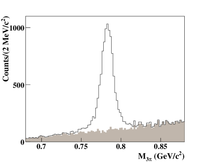
Figure 2: Mass of the $\pi^{+}\pi^{-}\pi^{0}$ system (GeV/c²) for all generated events (unshaded) and for only the background (shaded).

For the background, we chose to generate it according to 3-body phase space weighted by a linear function in $m_{3\pi}$ and

$$W(\theta,\phi)=\frac{1}{6\pi}\left(1+|\sin{\theta}\cos{\phi}|\right)$$ (15)

in the decay angles. When separating out the signal below, we assume we have no knowledge of Eq. 15 (this would typically be the case). Thus, the separation of signal and background will be carried out using only the knowledge that the background can be parametrized as a polynomial (with unknown parameters) in $m_{3\pi}$. No information about the distributions of the background in any other variables will be used. Figure 2 shows the $\pi^{+}\pi^{-}\pi^{0}$ mass spectrum for all generated events and for just the background. The generated decay angular distributions for all events, along with only the signal and background are shown in Fig. 1. There is clearly no selection criteria which can separate out the signal.

5.1 Applying the Procedure

To obtain the $Q$-factors, we first need to identify the relevant coordinates, i.e. the kinematic variables in which we need to separate signal from background. The $\pi^{+}\pi^{-}\pi^{0}$ mass will be used as the reference coordinate, $\xi_{r}\equiv m_{3\pi}$. The stated goal of our analysis is to extract the $\rho^{0}_{MM^{\prime}}$ elements. We will do this using Eq. (5); thus, only the angles $\theta,\phi$ are relevant. Other decay variables, such as the distance from the edge of the $\pi^{+}\pi^{-}\pi^{0}$ Dalitz plot, are not relevant to this analysis — though, they would be in other analyses (see Section 5.5).

Using the notation of Section 2, $\vec{\xi}=(m_{3\pi},\cos{\theta},\phi)$. The RMS’s of the relevant kinematic variables are

$$\sigma^{2}_{\phi}=\int_{-\pi}^{\pi}\phi^{2}d\phi=2\pi^{3}/3\\$$ (16a)

$$\sigma^{2}_{\cos{\theta}}=\int_{-1}^{1}\cos^{2}{\theta}d\cos{\theta}=2/3.$$ (16b)

The distance between any two points, $d_{ij}$, is then given by

$$d^{2}_{ij}=\frac{3}{2}\left[(\cos{\theta_{i}}-\cos{\theta_{j}})^{2}+\frac{(\phi_{i}-\phi_{j})^{2}}{\pi^{3}}\right].$$ (17)

The functional dependence of the signal and background on the reference coordinate, $m_{3\pi}$, are

$$F_{s}(m_{3\pi},\vec{\alpha})=s\cdot V(m_{3\pi},m_{\omega},\Gamma_{\omega},\sigma)$$ (18a)

$$F_{b}(m_{3\pi},\vec{\alpha})=b_{1}m_{3\pi}+b_{0},$$ (18b)

where $m_{\omega}=782.56$ MeV/c², $\Gamma_{\omega}=8.44$ MeV, ${\sigma=5}$ MeV is the simulated detector resolution, ${\vec{\alpha}=(s,b_{1},b_{0})}$ are unknown parameters and

$$V(m_{3\pi},m_{\omega},\Gamma_{\omega},\sigma)=\frac{1}{\sqrt{2\pi}\sigma}Re\left[w\left(\frac{1}{2\sqrt{\sigma}}(m_{3\pi}-m_{\omega})+i\frac{\Gamma_{\omega}}{2\sqrt{2}\sigma}\right)\right],$$ (19)

is the convolution of a Gaussian and non-relativistic Breit-Wigner known as a Voigtian ($w(z)$ is the complex error function).

As stated above, the number of nearest neighbor events required depends on the analysis. Specifically, it depends on how many unknown parameters there are, along with the functional forms of $F_{s}$ and $F_{b}$. For this relatively simple case, the value $n_{c}=100$ works well (see Section 5.4 for discussion on the value of $n_{c}$). For each simulated event, we then find the $n_{c}$ closest events (containing both signal and background events) and perform an unbinned maximum likelihood fit, using the CERNLIB package MINUIT [9], to determine the estimators $\hat{\alpha}$. The $Q$-factors are then calculated from Eq. (4) and the uncertainties are straightforward to calculate following Section 3.

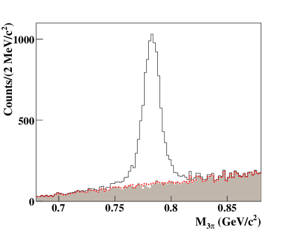
Figure 3: (Color Online) Mass of the $\pi^{+}\pi^{-}\pi^{0}$ system (GeV/c²) for all generated events (unshaded), only generated background events (shaded) and all generated events weighted by $1-Q$ (dashed-red).

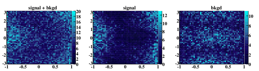
Figure 4: (Color Online) $\phi$ (radians) vs $\cos{\theta}$: Extracted decay angular distributions for all events (left), for events weighted by $Q$, signal (middle), and for events weighted by $1-Q$, background (right).

Figure 3 shows the comparison of the extracted and generated background $m_{3\pi}$ distributions integrated over all decay angles. The agreement is quite good; however, we are looking for more than just global agreement. Figure 4 shows the extracted angular distributions for the signal and background. The agreement with the generated distributions is excellent (see Fig. 1). A two-dimensional $\chi^{2}$ calculation comparing the generated and fit signal histograms yields $\chi^{2}/$ndf = 0.65 (where ndf is the degrees of freedom). This comparison may not be ideal due to the relatively large errors which exist on the small bin occupancies; however, it is sufficient to demonstrate the quality of the signal-background separation. We can also compare the $Q$-factors extracted by the fits to the theoretical distributions from which our data was generated. Figure 5 shows that the extracted values are in very good agreement with the generated ones.

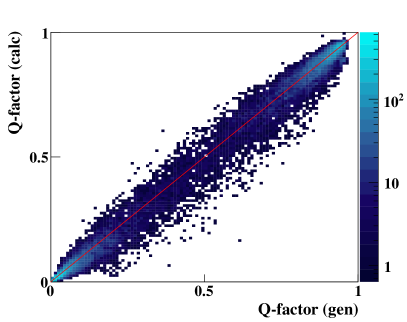
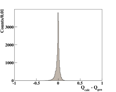
Figure 5: (Color Online) (a) Calculated $Q$-factors vs generated $Q$-factors. The red line indicates where ${Q_{calc}=Q_{gen}}$. (b) ${Q_{calc}-Q_{gen}}$: The difference between the generated and calculated $Q$-factors.

We conclude this section by discussing the importance of quality control in the fits. For this example, we performed 20,000 independent fits to extract the $Q$-factors. To avoid problems which can arise due to fits not converging or finding local minima, each unbinned maximum likelihood fit was run with three different sets of starting values for the parameters $\vec{\alpha}$: (1) 100% signal; (2) 100% background; (3) 50% signal, 50% background. In all cases, the fit with the best likelihood was used. The $n_{c}$ events were then binned and a $\chi^{2}/$ndf was obtained. In about 2% of the fits the $\chi^{2}/$ndf was very large, a clear indicator that the fit had not found the best estimators $\hat{\alpha}$. For these cases, a binned $\chi^{2}$ fit was run to obtain the $Q$-factor.

5.2 Examining the Errors

As discussed in Section 3, the covariance matrix obtained from each event’s fit can be used to obtain the uncertainty in $Q$, $\sigma_{Q}$, using Eq. (6). The nature of our procedure leads to a high degree of correlation between neighboring events’ $Q$-factors. This means that adding the uncertainties in quadrature would definitely underestimate the true error if the data is binned. In Section 3, we showed how to properly handle these uncertainties and also argued that a decent approximation could be obtained by assuming 100% correlation which provides an overestimate of the true error.

To examine the error bars in our toy example, we chose to project our data into a one-dimensional distribution in $\cos{\theta}$. This was done to avoid bin occupancy issues which arise in the two-dimensional case due to limitations in statistics. Figure 6(a) shows the comparison between the generated and calculated $\cos{\theta}$ distributions. The agreement is excellent. The error bars on the calculated points were obtained using Eq. (7). For this study, we ignore the Poisson statistical uncertainty in the yield due to the fact that the number of generated events is known. In a real world analysis, these should be included in the quoted error bars.

We can examine the quality of the error estimation by examining the difference between the generated and calculated yields in each bin, $\Delta\mathcal{Y}$. Figure 6(b) shows the comparison between $\Delta\mathcal{Y}$, $\sigma_{\mathcal{Y}}$ obtained using Eq. (7) and $\sigma_{\mathcal{Y}}$ obtained assuming 100% correlation. As expected, the 100% correlated errors provide an overestimate of $\Delta\mathcal{Y}$ in every bin, while the errors obtained using Eq. (7) provide an accurate calculation of the uncertainties.

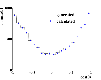
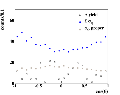
Figure 6: (Color Online) (a) Signal yield vs $\cos{\theta}$ for generated signal events (dashed) and all generated events weighted by $Q$-factors (blue circles). The error bars on the extracted yields were obtained using (7). (b) Comparison of the true error on the signal yield, $\Delta\mathcal{Y}=|\mathcal{Y}_{gen}-\mathcal{Y}_{calc}|$ (open black squares), to the error bars obtained using Eq. (7) (gray squares) and Eq. (8) (blue circles).

5.3 Extracting Observables

The goal of our model analysis is to extract the spin density matrix elements. Binning the data would be undesirable due to limitations in statistics. Following Section 4, we can instead perform an event-based maximum likelihood fit employing the $Q$-factors to handle the presence of background in our data set. The log likelihood is obtained from Eq. 12 as

$$-\ln{\mathcal{L}}=-\sum\limits_{i}^{n}Q_{i}\ln{W(\theta_{i},\phi_{i})},$$ (20)

where the sum is over all events (which contains signal and background). Using the $Q$-factors obtained in Section 5.1, minimizing Eq. (20) yields

$$\rho^{0}_{00}=0.659\pm 0.011$$ (21a)

$$\rho^{0}_{1-1}=0.044\pm 0.008$$ (21b)

$$Re\rho^{0}_{10}=0.108\pm 0.007,$$ (21c)

where the uncertainties are purely statistical (obtained from the fit covariance matrix). The values extracted for the spin density matrix elements are in excellent agreement with the values used to generate the data given in Eq. (14). To verify the accuracy of the statistical uncertainties, an ensemble of 100 example datasets was generated and the analysis procedure repeated on each independently. The pull distributions obtained for the spin density matrix elements are shown in Fig. 7. The means and widths are consistent with the expected values. Thus, no bias is found in the extracted observables and the statistical uncertainties obtained from the fits are correct.

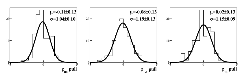
Figure 7: Pull distributions for the spin density matrix elements extracted from an ensemble of datasets generated from the signal and background PDF’s given in Section 5. The means and widths of the distributions are consistent with the expected values (0 and 1, respectively).

5.4 Choosing a Metric and a Value for $n_{c}$

In this section, we will examine the choices of the metric and of the value of $n_{c}$ (the number of nearest neighbor events used to determine the $Q$-factors). As stated above, it is not possible to provide general prescriptions for the metric and the value of $n_{c}$ that will guarantee the validity of the method for every analysis. Instead, these choices must be studied using the data and Monte Carlo data. Figure 8(a) shows the average relative uncertainty in $Q$ for different choices of $n_{c}$. As expected, this uncertainty increases as $n_{c}$ decreases. Keeping this uncertainty as small as possible dictates choosing a large value for $n_{c}$. If, however, $n_{c}$ is large relative to $n$, then the method will average over large fractions of phase space. This can result in losses of the finer structure in the distributions. Thus, there are two competing factors which should be considered when choosing the value of $n_{c}$. The ratio of $n_{c}/n$ must be small enough to permit a true extraction of the finer structure; however, the value of $n_{c}$ must be large enough such that the relative uncertainties in $Q$ are not too large. These constraints are analogous to those used to choose a bin width in a binned analysis.

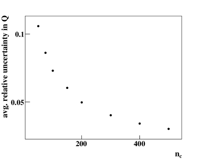
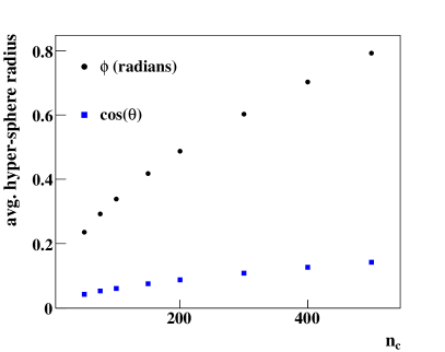
Figure 8: (a) Average relative uncertainty in $Q$ vs $n_{c}$. (b) Average hyper-sphere radius vs $n_{c}$.

Figure 8(a) shows that statistical fluctuations in the $Q$-factors become large (relative to variations in the physics) for $n_{c}<100$. Figure 8(b) shows the average radius (in $\phi$ and $\cos{\theta}$) of the hyper-spheres used to collect the $n_{c}$ events for different choices of $n_{c}$. From Fig. 4 we can estimate the size of the regions of phase space which are small enough such that the finer structure of the distributions is not lost. We then conclude that the choice $n_{c}\leq 200$ results in sufficiently small hyper-spheres. Following the ad-hoc prescription discussed above, we combine these two constraints which results in $100\leq n_{c}\leq 200$. Figure 9(a) shows a comparison of the $Q$-factors obtained using $n_{c}=100$ and $n_{c}=200$. There is no apparent structure and the fluctuations are consistent with the uncertainties on the $Q$-factors. Thus, the signal distributions reconstructed from these two choices of $n_{c}$ are statistically consistent. The spin density matrix elements extracted using the $Q$-factors obtained with $n_{c}=200$ are listed in Table 1. The values are very close to those obtained using $n_{c}=100$ in Section 5.3 and well within the statistical uncertainties.

We now want to examine the effects of choosing a different metric. In the previous sections, the RMS’s of the variables were used in Eq. (1) to determine the distance between events. Another possible choice would be to simply use the range of the variables, i.e. replace $\sigma_{\cos{\theta}}$ by 2 and $\sigma_{\phi}$ by $2\pi$. Figure 9(b) shows a comparison of the $Q$-factors obtained using RMS’s in the metric and those obtained using ranges. We again conclude that the signal distributions reconstructed from these two choices are statistically consistent. The spin density matrix elements extracted using the $Q$-factors obtained with this alternative metric are listed in Table 1. The results are again very close to those obtained in Section 5.3.

For this example, there is no physics-based motivation for adding dependence on the coordinates to the metric; however, to further demonstrate the robustness of the method, we can replace the RMS’s in Eq. (1) by the folloing quantities:

$$\sigma^{2}_{\phi}\rightarrow\left(\frac{2\pi^{3}}{3}\right)\left(1-\frac{3\phi^{2}}{4\pi^{2}}\right),\qquad\sigma^{2}_{\cos{\theta}}\rightarrow\left(\frac{2}{3}\right)\left(1-\frac{3}{4}\cos^{2}{\theta}\right).$$ (22)

The spin density matrix elements extracted using the $Q$-factors obtained with this alternative variable metric are listed in Table 1. The results are again very close to those obtained in Section 5.3. Therefore, the extracted observables are stable provided the choices of metric and $n_{c}$ obey the ad-hoc constraints discussed above.

	generated	signal	$n_{c}=100$ [“RMS” : ”range” : ”var”]	$n_{c}=200$[“RMS”]
$\rho^{0}_{00}$	0.65	0.649	[0.659 : 0.656 : 0.657]	0.656
$\rho^{0}_{1-1}$	0.05	0.043	[0.044 : 0.044 : 0.043]	0.042
$Re\rho^{0}_{10}$	0.10	0.103	[0.108 : 0.108 : 0.107]	0.107

Table 1: $\rho^{0}_{MM^{\prime}}$ values (fit and generated): The signal results were obtained by fitting only the generated signal events (unweighted). “RMS” refers to the metric constructed using the RMS’s of the variables in Eq. (1), “range” refers to simply using the ranges of the variables, and “var” refers to the variable metric constructed using Eq. (22) (see text for details). The statistical uncertainties on the extracted quantities are $\sigma_{00}=0.011$, $\sigma_{1-1}=0.008$ and $\sigma_{10}=0.007$ for each of the fit conditions.

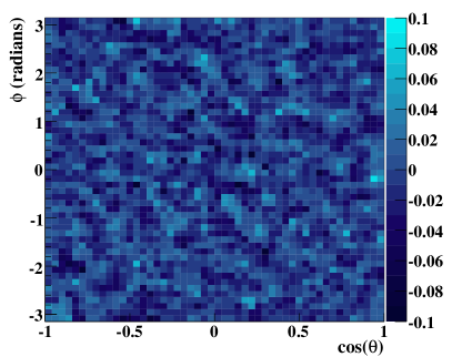
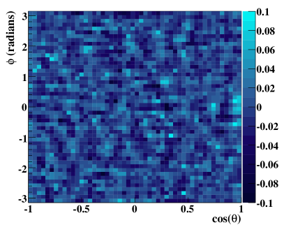
Figure 9: (Color Online) (a) $\Delta Q$ vs. $\phi$ (radians) vs. $\cos{\theta}$: Mean difference between the $Q$-factors extracted using $n_{c}=100$ and $n_{c}=200$. (b) $\Delta Q$ vs. $\phi$ (radians) vs. $\cos{\theta}$: Mean difference between the $Q$-factors extracted using RMS’s and ranges (see text for details) in the metric. In both cases, the differences in the $Q$-factors are consistent with their statistical uncertainties, i.e. there is no sensitivity in the reconstructed signal distributions to these choices of $n_{c}$ or metric.

5.5 Extending the Example

To extend this example to allow for the case where the data is not binned in production angle, we would simply need to include $\cos{\theta^{\omega}_{CM}}$ or $t$ in the vector of relevant coordinates, $\vec{\xi}$. To perform a full partial wave analysis on the data, we would also need to include any additional kinematic variables which factor into the partial wave amplitudes, e.g. the distance from the edge of the $\pi^{+}\pi^{-}\pi^{0}$ Dalitz plot (typically included in the $\omega$ decay amplitude). We would then construct the likelihood from the partial waves and minimize $-\ln{\mathcal{L}}$ using the $Q$-factors obtained by applying our procedure including the additional coordinates. An example of this can be found in [10].

6 Conclusions

In this paper, we have presented a procedure for separating signals from non-interfering backgrounds by determining, on an event-by-event basis, a quality factor ($Q$-factor) that a given event originated from the signal distribution. This procedure is a generalization of the side-band subtraction method to higher dimensions which does not require any binning of the data. We have shown that the $Q$-factors can be used as event weights in subsequent analysis procedures to allow more direct access to the true signal distribution. For example, the $Q$-factors can be used to weight the log likelihood in event-based unbinned maximum likelihood fits. This leads to background subtraction which is carried out automatically during the fits.

The method presented in this paper is meant to be applied to analyses where the distributions of the signal and background are unknown. All that is required is that each can be parametrized in terms of (at least) one coordinate which must not be correlated with the remaining set of coordinates. While it may be possible to overcome this limitation (i.e. it may be possible to account for the correlations in the PDFs), this topic is not explored in this paper as it is likely to be very problem specific. No knowledge about the distributions of the signal or background in any other coordinates is necessary.

The validity of the method depends on the choices of two ad-hoc quantities: the metric and the number of nearest-neighbor events used to define each hyper-sphere. It is not possible to provide general prescriptions for these quantities that will guarantee the validity of the method for every analysis. Instead, they must be studied using the data and Monte Carlo data for each analysis individually to confirm that the method produces valid results. The correlation distance varies according to the non-reference coordinates which makes proper handling of the errors an intricate task. Thus, the accuracy of the uncertainties on physical observables extracted from the data should be verified by a Monte Carlo study as well. Given these caveats, it is clear that performing a detailed study using Monte Carlo data is an important prerequisite to using this method for any analysis.

- [1] I. Narsky, in PHYSTATO5: Statistical Problems in Particle Physics, proceedings of the international conference, Oxford, England, United Kingdom (2005).
- [2] K. Cranmer, in PHYSTATO5: Statistical Problems in Particle Physics, proceedings of the international conference, Oxford, England, United Kingdom (2005).
- [3] R. Vilalta, in PHYSTATO5: Statistical Problems in Particle Physics, proceedings of the international conference, Oxford, England, United Kingdom (2005).
- [4] T. Hastie, R. Tibshirani and J. Friedman, The Elements of Statistical Learning: Data Mining, Inference, and Prediction. Springer-Verlag, 2001.
- [5] M. Pivk and F. R. Le Diberder, Nucl. Instrum. Meth. A 555, 356 (2005).
- [6] A. L. Read, CERN-OPEN-2000-205 (2000).
- [7] S. S. Chen and R. A. Gopinath, Advances in Neural Information Processing Systems 13 (2001).
- [8] K. Schilling, P. Seyboth and G. Wolf, Nucl. Phys. B15, 397 (1970).
- [9] F. James, CERN Program Library D506 (1998).
- [10] M. Williams, Ph.D. thesis, Carnegie Mellon University, 2007.