Exponential functionals of Brownian motion and class-one Whittaker functions

Abstract

We consider exponential functionals of a Brownian motion with drift in ${\mathbb{R}}^{n}$, defined via a collection of linear functionals. We give a characterisation of the Laplace transform of their joint law as the unique bounded solution, up to a constant factor, to a Schrödinger-type partial differential equation. We derive a similar equation for the probability density. We then characterise all diffusions which can be interpreted as having the law of the Brownian motion with drift conditioned on the law of its exponential functionals. In the case where the family of linear functionals is a set of simple roots, the Laplace transform of the joint law of the corresponding exponential functionals can be expressed in terms of a (class-one) Whittaker function associated with the corresponding root system. In this setting, we establish some basic properties of the corresponding diffusion processes.

1 Introduction

Let $(X_{t},t\geq 0)$ be a standard one-dimensional Brownian motion with drift $\mu$. In the paper [19], Matsumoto and Yor consider the process

$$\left(\log\int_{0}^{t}e^{2X_{s}-X_{t}}ds,\ t>0\right),$$

and prove that it is a diffusion process with infinitesimal generator given by

$$\frac{1}{2}\frac{d^{2}}{dx^{2}}+\left(\frac{d}{dx}\log K_{\mu}(e^{-x})\right)\frac{d}{dx},$$ (1)

where $K_{\mu}$ is the Macdonald function. As explained in [19], this theorem can be regarded, by Brownian scaling and Laplace’s method, as a generalization of Pitman’s ‘$2M-X$’ theorem [26, 27] which states that, if $M_{t}=\max_{0\leq s\leq t}X_{s}$, then $2M-X$ is a diffusion process with infinitesimal generator given by

$$\frac{1}{2}\frac{d^{2}}{dx^{2}}+\mu\coth(\mu x)\frac{d}{dx}.$$ (2)

Note that $\mu\coth(\mu x)=(-\mu)\coth(-\mu x)$ and $K_{\mu}=K_{-\mu}$. Suppose $\mu>0$. Then the diffusion with generator (2) can be interpreted as a Brownian motion with drift $\mu$ conditioned to stay positive. Similarly, the diffusion with generator (1) can be interpreted as the Brownian motion $X$ conditioned on its exponential functional $A=\int_{0}^{\infty}e^{-2X_{s}}ds$ having a certain distribution (a Generalised Inverse Gaussian law) in a sense which can be made precise [2, 3]. The relevance of these interpretations in the present context is as follows.

Set $J=-\min_{t\geq 0}X_{t}$ and let $\tilde{J}$ be an independent copy of $J$ which is also independent of $X$. Then the process $\tilde{X}=2\max\{M-\tilde{J},0\}-X$ has the same law as $X$ and, moreover, $\tilde{J}=-\min_{t\geq 0}\tilde{X}_{t}$. This is well-known and can be seen for example as a consequence of the classical output theorem for the $M/M/1$ queue [24]. From this we can see that the process $2M-X$ has the same law as that of $X$ conditioned (in an appropriate sense) on the event that $J=0$; in other words, $2M-X$ is a diffusion with infinitesimal generator given by (2), started from zero. This basic idea can be used to obtain a multi-dimensional version of Pitman’s $2M-X$ theorem [4, 5, 25], which gives a representation of a Brownian motion conditioned to stay in a Weyl chamber in ${\mathbb{R}}^{n}$ as a certain functional (which generalizes $2M-X$) of a Brownian motion in ${\mathbb{R}}^{n}$.

Similarly [19], if $\tilde{A}$ is an independent copy of $A$, which is also independent of $X$, then the process

$$\tilde{X}_{t}=\log\left(1+\tilde{A}^{-1}\int_{0}^{t}e^{2(X_{s}-X_{t})}ds\right)+X_{t},\qquad t\geq 0$$

has the same law as $X$ and, moreover, $\tilde{A}=\int_{0}^{\infty}e^{-2\tilde{X}_{s}}ds$. This time, we conclude that, for each $\epsilon>0$, the process

$$\log\left(\epsilon+\int_{0}^{t}e^{2(X_{s}-X_{t})}ds\right)+X_{t},\qquad t\geq 0$$

the same law as that of $\log\epsilon+X$ conditioned on the event $A=\epsilon$. Carefully letting $\epsilon\to 0$ yields the theorem of Matsumoto and Yor [2]. As explained in [22], the probabilistic proofs of the multi-dimensional versions of Pitman’s $2M-X$ theorem given in the papers [4, 25] carry over, in the same way, to the exponential functionals setting, although the task of letting the analogue of $\epsilon$ go to zero is a highly non-trivial problem in the general setting. Nevertheless, it gives a heuristic derivation that a certain functional of a Brownian motion in ${\mathbb{R}}^{n}$ should have the same law as a Brownian motion conditioned on a certain collection of its exponential functionals. This leads us to the question considered in the present paper.

We consider a Brownian motion $B^{(\mu)}$ in ${\mathbb{R}}^{n}$ with drift $\mu$, and a collection of linear functionals $\alpha_{1},\ldots,\alpha_{d}$ such that the exponential functionals

$$A^{i}_{\infty}=\int_{0}^{\infty}e^{-2\alpha_{i}(B_{s}^{(\mu)})}ds\qquad(i=1,\ldots,d)$$

are almost surely finite. Our aim is to understand which diffusion processes can arise when we condition on the law of $A_{\infty}=(A^{1}_{\infty},\ldots,A^{d}_{\infty})$. The first step is to understand the law of $A_{\infty}$. We show that the Laplace transform of $A_{\infty}$ satisfies a certain Schrödinger-type partial differential equation and proceed to characterise all diffusion processes which can be interpreted as having the law of $B^{(\mu)}$ conditioned on the law of $A_{\infty}$.

In the case when $\alpha_{1},\ldots,\alpha_{d}$ is a simple system (see section 4 below for a definition), these diffusion processes are closely related to the quantum Toda lattice. The Schrödinger operator is

$$H=\frac{1}{2}\Delta+\sum_{i}\theta_{i}^{2}e^{-2\alpha_{i}},$$

where $\theta\in{\mathbb{R}}^{d}$, and the corresponding diffusion process has infinitesimal generator given by

$$\frac{1}{2}\Delta+\nabla\log k_{\mu}\cdot\nabla,$$ (3)

where $k_{\mu}$ is a particular eigenfunction of $H$ known as a class-one Whittaker function. In the case $n=d=1$ and $\alpha_{1}(x)=x$, the class-one Whittaker function is $k_{\mu}(x)=K_{\mu}(e^{-x})$ and the infinitesimal generator is given by (1). More generally, for a simple system $\alpha_{1},\ldots,\alpha_{d}$, the diffusion process with generator given by (3) plays an analogous role, in the exponential functionals setting, as that of a Brownian motion conditioned to stay in the Weyl chamber $\{x\in{\mathbb{R}}^{n}:\ \alpha_{i}(x)>0,\ i=1,\ldots,d\}$. These processes have already found an application in the paper [23], where the corresponding multi-dimensional version of the above theorem of Matsumoto and Yor in the ‘type A’ case has been proved and used to determine the law of the partition function associated with a directed polymer model which was introduced in the paper [24].

The outline of the paper is as follows. In section 2 we work in a general setting and establish a Schrödinger type partial differential equation satisfied by the characteristic function of exponential functionals of a multidimensional Brownian motion. We also study a family of martingales related to the conditional laws of exponential functionals that will later appear. In section 3, we identify a family of diffusions which can be interpreted as having the law of the Brownian motion with drift conditioned on the law of its exponential functionals. In section 4, we restrict our attention to the case where the collection of vectors used to define the exponential functionals is a simple system, and give an overview of relevant facts about class-one Whittaker functions. In section 5, we study properties of the conditioned processes in this setting. In the final section, we present some explicit results for the ‘type $A_{2}$’ case.

2 Exponential functionals and associated partial differential equations

In this section, we work in a general setting and establish a Schrödinger type partial differential equation satisfied by the characteristic function of exponential functionals of a multidimensional Brownian motion. We also study a family of martingales related to the conditional laws of exponential functionals that will later appear.

Let $\alpha_{1},\ldots,\alpha_{d}$ be a collection of distinct, non-zero vectors in ${\mathbb{R}}^{n}$ such that

$$\Omega=\{x\in{\mathbb{R}}^{n}:\ \alpha_{i}(x)>0\ \forall i\}$$ (4)

is non-empty. Let $B^{(\mu)}$ be a standard Brownian motion in ${\mathbb{R}}^{n}$ with drift $\mu\in\Omega$. For $0\leq t\leq\infty$, set

$$A^{i}_{t}=\int_{0}^{t}e^{-2\alpha_{i}(B_{s}^{(\mu)})}ds\qquad i=1,\ldots,d.$$

Here, $\alpha_{i}(\beta)=(\alpha_{i},\beta)$ where $(\cdot,\cdot)$ denotes the usual inner product on ${\mathbb{R}}^{n}$.

2.1 Partial differential equation for the characteristic function

The process $\left(B_{t}^{(\mu)},A_{t}\right)_{t\geq 0}$ is a diffusion with generator

$$\frac{1}{2}\Delta_{x}+(\mu,\nabla_{x})+\sum_{i=1}^{d}e^{-2\alpha_{i}(x)}\frac{\partial}{\partial a_{i}}.$$

We first check that this operator is hypoelliptic.

Proposition 2.1.

The operator

$$\frac{1}{2}\Delta_{x}+(\mu,\nabla_{x})+\sum_{i=1}^{d}e^{-2\alpha_{i}(x)}\frac{\partial}{\partial a_{i}}$$

is hypoelliptic on $\mathbb{R}^{n+d}$ and therefore, for $t>0$ the random variable $\left(B_{t}^{(\mu)},A_{t}\right)$ admits a smooth density with respect to the Lebesgue measure.

Proof.

We use Hörmander’s theorem. Since the $\alpha_{i}$’s are pairwise different and non zero, there exists $v\in\mathbb{R}^{n}$ such that

$$i\neq j\Rightarrow\alpha_{i}(v)\neq\alpha_{j}(v).$$

Consider now the vector field

$$V=\sum_{i=1}^{n}v_{i}\frac{\partial}{\partial x_{i}},$$

and let us denote

$$T=\sum_{i=1}^{d}e^{-2\alpha_{i}(x)}\frac{\partial}{\partial a_{i}}$$

The Lie bracket between $V$ and $T$ is given by

$$\mathcal{L}_{V}T=[V,T]=-2\sum_{i=1}^{d}\alpha_{i}(v)e^{-2\alpha_{i}(x)}\frac{\partial}{\partial a_{i}}.$$

Similarly, by iterating this bracket $k$ times, we get

$$\mathcal{L}^{k}_{V}T=(-1)^{k}2^{k}\sum_{i=1}^{d}\alpha_{i}(v)^{k}e^{-2\alpha_{i}(x)}\frac{\partial}{\partial a_{i}}.$$

Since the $\alpha_{i}$’s are pairwise different and non zero, we deduce from the Van der Monde determinant that at every $x\in\mathbb{R}^{n}$ the family

$$\left\{\mathcal{L}^{k}_{V}T,1\leq k\leq d\right\}.$$

is a basis of $\mathbb{R}^{d}$. It implies that the Lie bracket generating condition of Hörmander is sastisfied so that the operator $\frac{1}{2}\Delta_{x}+(\mu,\nabla_{x})+\sum_{i=1}^{d}e^{-2\alpha_{i}(x)}\frac{\partial}{\partial a_{i}}$ is hypoelliptic. ∎

Let now $\theta\in{\mathbb{R}}^{d}$ and, for $x\in\mathbb{R}^{n}$, define

$$g_{\mu}^{\theta}(t,x)=\mathbb{E}\left(e^{-\sum_{i=1}^{d}\theta_{i}^{2}e^{-2\alpha_{i}(x)}A_{t}^{i}}\right),\quad t\geq 0,$$

and

$$j_{\mu}^{\theta}(x)=\mathbb{E}\left(e^{-\sum_{i=1}^{d}\theta_{i}^{2}e^{-2\alpha_{i}(x)}A_{\infty}^{i}}\right).$$

Proposition 2.2.

1. The semigroup generated by the Schrödinger operator

   $$\frac{1}{2}\Delta+(\mu,\nabla)-\sum_{i=1}^{d}\theta_{i}^{2}e^{-2\alpha_{i}(x)}$$

   admits a heat kernel $q_{\mu}^{\theta}(t,x,y)$ and we have

   $$g_{\mu}^{\theta}(t,x)=\int_{\mathbb{R}^{n}}q_{\mu}^{\theta}(t,x,y)dy.$$

2. The function $j_{\mu}^{\theta}$ is the unique bounded function that satisfies the partial differential equation

   $$\frac{1}{2}\Delta j_{\mu}^{\theta}(x)+(\mu,\nabla j_{\mu}^{\theta}(x))=\left(\sum_{i=1}^{d}\theta_{i}^{2}e^{-2\alpha_{i}(x)}\right)j_{\mu}^{\theta}(x)$$

   and the limit condition

   $$\lim_{x\rightarrow\infty,x\in\Omega}j_{\mu}^{\theta}(x)=1.$$

Proof.

1. It is a straightforward consequence of the Feynman-Kac formula that $q_{\mu}^{\theta}(t,x,y)$ exists and is given by

   $$q_{\mu}^{\theta}(t,x,y)=\mathbb{E}\left(e^{-\sum_{i=1}^{d}\theta_{i}^{2}e^{-2\alpha_{i}(x)}A_{t}^{i}}\mid B_{t}^{(\mu)}=y-x\right)\frac{1}{(2\pi t)^{\frac{n}{2}}}e^{-\frac{\|y-x-\mu t\|^{2}}{2t}}.$$

   Integrating this with respect to $y$, we obtain

   $$g_{\mu}^{\theta}(t,x)=\int_{\mathbb{R}^{n}}q_{\mu}^{\theta}(t,x,y)dy.$$

2. It is again a straightforward consequence of the Feynman-Kac formula that $j_{\mu}^{\theta}$ solves the partial differential equation, and the limit condition is easily checked. Let us now prove uniqueness. We have to show that if $\phi$ is a bounded solution of the equation that satisfies

   $$\lim_{x\rightarrow\infty,x\in\Omega}\phi(x)=0,$$

   then $\phi=0$. For that, let us observe that under the above conditions, for $x\in\mathbb{R}^{n}$, the process

   $$\phi(B_{t}^{(\mu)}+x)\exp\left(-\sum_{i=1}^{d}\theta_{i}^{2}e^{-2\alpha_{i}(x)}A_{t}^{i}\right)$$

   is a bounded martingale that goes to 0 when $t\rightarrow+\infty$. It follows that this martingale is identically zero almost surely, which implies $\phi=0$.

∎

For later reference, we rephrase the second part of the previous proposition as follows:

Corollary 2.3.

The function $h_{\mu}^{\theta}(x)=e^{\mu(x)}j_{\mu}^{\theta}(x)$ is the unique solution to

$$\frac{1}{2}\Delta h_{\mu}^{\theta}(x)-\sum_{i=1}^{d}\theta_{i}^{2}e^{-2\alpha_{i}(x)}h_{\mu}^{\theta}(x)=\frac{1}{2}\|\mu\|^{2}h_{\mu}^{\theta}(x),$$ (5)

such that $e^{-\mu(x)}h_{\mu}^{\theta}(x)$ is bounded and

$$\lim_{x\rightarrow\infty,x\in\Omega}e^{-\mu(x)}h_{\mu}^{\theta}(x)=1.$$

Example 2.1.

The following example has been widely studied (see, for example, [8, 19] and references therein). Suppose $n=d=1$, $\theta_{1}^{2}=1/2$ and $\alpha_{1}(x)=x$. Then

$$A_{\infty}=\int_{0}^{\infty}e^{-2(B_{t}+\mu t)}dt,\quad\mu>0$$

where $(B_{t},\ t\geq 0)$ is a standard one-dimensional Brownian motion, and

$$j_{\mu}^{\theta}(x)={\mathbb{E}}\left(\exp\left(-\frac{1}{2}e^{-2x}A_{\infty}\right)\right)\qquad x\in{\mathbb{R}}.$$

In this case, $h_{\mu}^{\theta}(x)=e^{\mu x}j_{\mu}^{\theta}(x)$ solves the equation

$$\left(\frac{d^{2}}{dx^{2}}-e^{-2x}\right)h_{\mu}^{\theta}=\mu^{2}h_{\mu}^{\theta}$$

This equation is easily solved by means of Bessel functions. By taking into account the boundary condition when $x\rightarrow+\infty$, we recover the formula [19, Theorem 6.2]:

$$j_{\mu}^{\theta}(x)=\frac{2^{1-\mu}}{\Gamma(\mu)}e^{-\mu x}K_{\mu}(e^{-x}),$$ (6)

where $K_{\mu}$ is the Macdonald function [18]:

$$K_{\mu}(x)=\frac{1}{2}\left(\frac{x}{2}\right)^{\mu}\int_{0}^{+\infty}\frac{e^{-t-\frac{x^{2}}{4t}}}{t^{1+\mu}}dt.$$ (7)

The formula (6) can also be derived using the fact [8] that $A_{\infty}$ has the same law as $1/2\gamma_{\mu}$, where $\gamma_{\mu}$ is a gamma distributed random variable with parameter $\mu$.

Example 2.2.

The following example has also been studied in the literature [12, 14]. Suppose $n=1$, $d=2$, $\theta_{1}^{2}=\theta_{2}^{2}=1/2$, $\alpha_{1}(x)=x$ and $\alpha_{2}(x)=\frac{x}{2}$. Then

$$A^{1}_{\infty}=\int_{0}^{\infty}e^{-2(B_{t}+\mu t)}dt,\quad A^{2}_{\infty}=\int_{0}^{\infty}e^{-(B_{t}+\mu t)}dt,\quad\mu>0$$

where $(B_{t},\ t\geq 0)$ is a standard one-dimensional Brownian motion, and

$$j_{\mu}^{\theta}(x)={\mathbb{E}}\left(\exp\left(-\frac{1}{2}e^{-2x}A^{1}_{\infty}-\frac{1}{2}e^{-x}A^{2}_{\infty}\right)\right)\qquad x\in{\mathbb{R}}.$$

In this case, $h_{\mu}^{\theta}(x)=e^{\mu x}j_{\mu}^{\theta}(x)$ solves the equation

$$\left(\frac{d^{2}}{dx^{2}}-e^{-x}-e^{-2x}\right)h_{\mu}^{\theta}=\mu^{2}h_{\mu}^{\theta}$$

This is Schrödinger’s equation with the so-called Morse potential. It is solved by means of Whittaker functions and by taking into account the boundary condition when $x\rightarrow+\infty$, we get

$$j_{\mu}^{\theta}(x)=2^{\mu-\frac{1}{2}}\frac{\Gamma(1+\mu)}{\Gamma(2\mu)}e^{\left(-\mu+\frac{1}{2}\right)x}W_{-\frac{1}{2},\mu}(2e^{-x})$$

where $W_{k,\mu}$ is the Whittaker function (see [18, pp.279]):

$$W_{k,\mu}(x)=\frac{x^{k}e^{-\frac{x}{2}}}{\Gamma\left(\frac{1}{2}+\mu-k\right)}\int_{0}^{+\infty}e^{-t}t^{\mu-k-\frac{1}{2}}\left(1+\frac{t}{x}\right)^{\mu+k-\frac{1}{2}}dt.$$

2.2 Conditional densities

We prove now that the random variable $A_{\infty}$ has a smooth density with respect to the Lebesgue measure of $\mathbb{R}^{d}$ and morever give an expression of the conditional densities only in terms of this density.

Proposition 2.4.

The random variable $A_{\infty}$ has a smooth density $p$ with respect to the Lebesgue measure of $\mathbb{R}^{d}$ and for $t\geq 0$

$$\mathbb{P}(A_{\infty}\in dy\left|\mathcal{F}_{t}\right.)=e^{2\sum_{i=1}^{d}\alpha_{i}(B^{(\mu)}_{t})}p\left(e^{2\alpha_{1}(B^{(\mu)}_{t})}(y_{1}-A^{1}_{t}),\cdots,e^{2\alpha_{d}(B^{(\mu)}_{t})}(y_{d}-A^{d}_{t})\right)\mathbf{1}_{(0,y_{1})\times\cdots\times(0,y_{n})}(A_{t})dy$$

where $\mathcal{F}$ is the natural filtration of $B^{(\mu)}$.

Proof.

If we denote by $\phi$ the characteristic function of $A_{\infty}$:

$$\phi(\lambda)=\mathbb{E}\left(e^{-(\lambda,A_{\infty})}\right),\quad\lambda_{1},...,\lambda_{d}>0,$$

then,

$$\mathbb{E}\left(e^{-\sum_{i=1}^{d}\lambda_{i}A^{i}_{\infty}}\left|\mathcal{F}_{t}\right.\right) =e^{-\sum_{i=1}^{d}\lambda_{i}A^{i}_{t}}\mathbb{E}\left(e^{-\sum_{i=1}^{d}\lambda_{i}(A^{i}_{\infty}-A^{i}_{t})}\left|\mathcal{F}_{t}\right.\right)$$

$$=e^{-(\lambda,A_{t})}\phi\left(e^{-2\alpha_{1}(B^{(\mu)}_{t})}\lambda_{1},\cdots,e^{-2\alpha_{d}(B^{(\mu)}_{t})}\lambda_{d}\right).$$

Therefore, the process $e^{-(\lambda,A_{t})}\phi\left(e^{-2\alpha_{1}(B^{(\mu)}_{t})}\lambda_{1},\cdots,e^{-2\alpha_{d}(B^{(\mu)}_{t})}\lambda_{d}\right)$ is a martingale. This implies that the function $e^{-(\lambda,a)}\phi\left(e^{-2\alpha_{1}(x)}\lambda_{1},\cdots,e^{-2\alpha_{d}(x)}\lambda_{d}\right)$ is harmonic for the operator $\frac{1}{2}\Delta_{x}+(\mu,\nabla_{x})+\sum_{i=1}^{d}e^{-2\alpha_{i}(x)}\frac{\partial}{\partial a_{i}}$. This operator being hypoelliptic, this implies that $A_{\infty}$ has a smooth density with respect to the Lebesgue measure of $\mathbb{R}^{d}$. The result about the conditional densities stems from the injectivity of the Laplace transform. ∎

In particular, we deduce from the previous proposition that if for $y\in\mathbb{R}^{d}_{+}$, we denote

$$q(x,a,y)=e^{2\sum_{i=1}^{d}\alpha_{i}(x)}p\left(e^{2\alpha_{1}(x)}(y_{1}-a_{1}),\cdots,e^{2\alpha_{d}(x)}(y_{d}-a_{d})\right),$$

for $0<a_{i}<y_{i},x\in\mathbb{R}^{d}$, then the process $q\left(B_{t}^{(\mu)},A_{t},y\right)\mathbf{1}_{(0,y_{1})\times\cdots\times(0,y_{n})}(A_{t})$ is a martingale. It implies that for any $y\in\mathbb{R}^{d}_{+}$, $q(x,a,y)$ satisfies the following partial differential equation:

$$\frac{1}{2}\Delta_{x}q+(\mu,\nabla_{x}q)+\sum_{i=1}^{d}e^{-2\alpha_{i}(x)}\frac{\partial q}{\partial a_{i}}=0.$$

It also implies that $p$ is a solution of the partial differential equation:

$$\sum_{i,j=1}^{d}(\alpha_{i},\alpha_{j})y_{i}y_{j}\frac{\partial^{2}p}{\partial y_{i}\partial y_{j}}+\sum_{i=1}^{d} \left(\left(\alpha_{i}(\mu)+\|\alpha_{i}\|^{2}+2\sum_{j=1}^{d}(\alpha_{i},\alpha_{j})\right)y_{i}-\frac{1}{2}\right)\frac{\partial p}{\partial y_{i}}$$

$$= -\left(\sum_{i,j=1}^{d}(\alpha_{i},\alpha_{j})+\sum_{i=1}^{d}\alpha_{i}(\mu)\right)p.$$

Example 2.3.

Suppose $n=d=1$, $\theta_{1}^{2}=1/2$ and $\alpha_{1}(x)=x$. Then $A_{\infty}$ is distributed as $1/2\gamma_{\mu}$, where $\gamma_{\mu}$ is a gamma law with parameter $\mu$, that is

$$p(y)=\frac{1}{2^{\mu}\Gamma(\mu)}\frac{e^{-\frac{1}{2y}}}{y^{1+\mu}}1_{\mathbb{R}_{>0}}(y),$$

and we have

$$q(x,a,y)=\frac{1}{2^{\mu}\Gamma(\mu)}\frac{e^{-2\mu x-\frac{1}{2}\frac{e^{-2x}}{y-a}}}{(y-a)^{1+\mu}}1_{\mathbb{R}_{>0}}(y-a)$$

Example 2.4.

Suppose $n=1$, $d=2$, $\alpha_{1}(x)=x$ and $\alpha_{2}(x)=\frac{x}{2}$. Then, as seen before,

$$A^{1}_{\infty}=\int_{0}^{\infty}e^{-2(B_{t}+\mu t)}dt,\quad A^{2}_{\infty}=\int_{0}^{\infty}e^{-(B_{t}+\mu t)}dt,\quad\mu>0,$$

and for $\lambda_{1},\lambda_{2}>0$,

$$\mathbb{E}\left(e^{-\frac{1}{2}\lambda_{1}^{2}A_{1}^{\infty}-\frac{1}{2}\lambda_{2}^{2}A_{2}^{\infty}}\right) =2^{\mu-\frac{1}{2}}\lambda_{1}^{\mu-\frac{1}{2}}\frac{\Gamma\left(\mu+\frac{1}{2}+\frac{\lambda_{2}^{2}}{2\lambda_{1}}\right)}{\Gamma(2\mu)}W_{-\frac{\lambda_{2}^{2}}{2\lambda_{1}},\mu}(2\lambda_{1})$$

$$=\frac{e^{-\lambda_{1}}}{\Gamma(2\mu)}\int_{0}^{+\infty}e^{-t}t^{\mu+\frac{\lambda_{2}^{2}}{2\lambda_{1}}-\frac{1}{2}}(2\lambda_{1}+t)^{\mu-\frac{\lambda_{2}^{2}}{2\lambda_{1}}-\frac{1}{2}}dt.$$

By using in the previous integral the change of variable $t=\frac{2\lambda_{1}}{e^{\lambda_{1}s}-1}$, we deduce the following nice formula

$$\mathbb{E}\left(e^{-\frac{1}{2}\lambda_{1}^{2}A^{1}_{\infty}}\mid A_{\infty}^{2}=s\right)\mathbb{P}(A^{2}_{\infty}\in ds)=\frac{\lambda_{1}^{2\mu+1}}{2\Gamma(2\mu)}\frac{e^{-\lambda_{1}\mathrm{cotanh}\frac{\lambda_{1}s}{2}}}{\left(\sinh\frac{\lambda_{1}s}{2}\right)^{2\mu+1}}ds,\quad s>0.$$

This conditional Laplace transform can be inverted (see for instance [9]) but, unlike the one-dimensional case, it does not seem to lead to a nice formula for $p$:

$$p(y_{1},y_{2})=\frac{2^{2\mu}}{\Gamma(2\mu)\sqrt{2\pi}}\sum_{j,k=0}^{+\infty} \frac{(-1)^{j}2^{j}}{j!}\frac{\Gamma(j+2\mu+1+k)}{k!\Gamma(j+2\mu+1)}\frac{1}{y_{1}^{\frac{j}{2}+\mu+\frac{3}{2}}}e^{-\frac{(1+y_{2}(k+j+\mu+\frac{1}{2}))^{2}}{4y_{1}}}$$

$$\times D_{j+2\mu+2}\left(\frac{1+y_{2}(k+j+\mu+\frac{1}{2})}{\sqrt{y_{1}}}\right)$$

where $D_{\nu}$ is the parabolic cylinder function such that

$$\int_{0}^{+\infty}\frac{e^{-\theta t}}{t^{1+\nu}}e^{-\frac{a^{2}}{4t}}D_{2\nu+1}\left(\frac{a}{\sqrt{t}}\right)dt=\sqrt{\pi}2^{\nu+\frac{1}{2}}\theta^{\nu}e^{-a\sqrt{2\theta}},$$

that is

$$D_{\nu}(x)=\frac{\sqrt{2}}{\sqrt{\pi}}e^{\frac{x^{2}}{4}}\int_{0}^{+\infty}t^{\nu}e^{-\frac{t^{2}}{2}}\cos\left(xt-\frac{\pi\nu}{2}\right)dt,\quad\nu>-1$$

3 Brownian motion conditioned on its exponential functionals

In this section, we study the Doob transforms of the process $\left(B_{t}^{(\mu)},A_{t}\right)$ associated with the conditioning of $A_{\infty}$. We first start with the bridges which are the extremal points.

Lemma 3.1 (Equation of the bridges).

Let $y\in\mathbb{R}_{+}^{d}$. The law of the process $(B_{t}+\mu t)_{t\geq 0}$ conditioned by

$$A_{\infty}=y$$

solves the following stochastic differential equation:

$$dX_{t}=\left(\mu+(\nabla_{x}\ln q)\left(X_{t},\int_{0}^{t}e^{-2\alpha(X_{s})}ds,y\right)\right)dt+d\beta_{t}$$

where, $(\beta_{t})_{t\geq 0}$ is a standard Brownian motion

Proof.

This follows directly from Proposition 2.4 and Girsanov’s theorem. ∎

Example 3.1.

The following example is considered [21]. Suppose $n=d=1$, $\theta_{1}^{2}=1/2$ and $\alpha_{1}(x)=x$. Then the equation becomes

$$dX_{t}=\left(-\mu+\frac{e^{-2X_{t}}}{y-\int_{0}^{t}e^{-2X_{s}}ds}\right)dt+d\beta_{t}.$$

Let $\mathbb{P}^{\mu}$ be the law of $B^{(\mu)}$ and $\pi$ be the coordinate process on the space of continuous functions $\mathbb{R}_{+}\rightarrow\mathbb{R}^{n}$. If $\nu$ is a probability measure on $\mathbb{R}^{d}_{+}$, in what follows (see [3]), we call the probability

$$\int_{\mathbb{R}^{d}_{+}}\mathbb{P}^{\mu}\left(\quad\cdot\quad\left|\int_{0}^{+\infty}e^{-2\alpha_{1}(\pi_{s})}ds=y_{1},\cdots,\int_{0}^{+\infty}e^{-2\alpha_{d}(\pi_{s})}ds=y_{d}\right)\right.\nu(dy),$$

the law of the process $(B_{t}+\mu t)_{t\geq 0}$ conditioned by

$$A_{\infty}=^{law}\nu.$$

Proposition 3.1.

Let $v$ be a bounded and positive function such that $\int_{\mathbb{R}^{d}}v(y)p(y)dy=1$. The law of the process $(B_{t}+\mu t)_{t\geq 0}$ conditioned by

$$A_{\infty}=^{law}v(x)p(x)dx$$

solves the following stochastic differential equation:

$$dX_{t}=\left(\mu+F_{v}\left(\int_{0}^{t}e^{-2\alpha_{1}(X_{s})}ds,\cdots,\int_{0}^{t}e^{-2\alpha_{d}(X_{s})}ds,X_{t}\right)\right)dt+d\beta_{t}$$

where, $(\beta_{t})_{t\geq 0}$ is a standard Brownian motion and $F_{v}:\mathbb{R}^{d}\times\mathbb{R}^{n}\rightarrow\mathbb{R}^{n}$ is given by

$$F_{v}(a,x)=(\nabla_{x}\ln\phi_{v})(a,x)$$

with

$$\phi_{v}(a,x)=\int_{\mathbb{R}^{d}}p(z)v\left(a_{1}+e^{-2\alpha_{1}(x)}z_{1},\cdots,a_{d}+e^{-2\alpha_{d}(x)}z_{d}\right)dz.$$

Proof.

Following [3], we have to write the stochastic differential equation associated with the conditioning

$$A_{\infty}=^{law}p(x)v(x)dx.$$

But

$$\mathbb{E}\left(v\left(A_{\infty}\right)\left|\mathcal{F}_{t}\right.\right)= e^{2\sum_{i=1}^{d}\alpha_{i}(B^{(\mu)}_{t})}\int_{\mathbb{R}^{d}}p\left(e^{2\alpha_{1}(B^{(\mu)}_{t})}(y_{1}-A^{1}_{t}),\cdots,e^{2\alpha_{d}(B^{(\mu)}_{t})}(y_{d}-A^{d}_{t})\right)v(y)dy$$

$$= \phi_{v}(A_{t},B_{t}^{(\mu)}),$$

so that we get the expected conditioned stochastic differential equation by Girsanov theorem.

∎

In the previous proposition, the drift $F_{v}(a,x)$ depends only on $x$ if, and only if,

$$v(x)=\frac{e^{-\sum_{i=1}^{d}\theta_{i}^{2}x_{i}}}{j_{\mu}^{\theta}(0)},$$

for some $\theta\in\mathbb{R}^{d}$. Therefore:

Corollary 3.2.

For $\theta\in\mathbb{R}^{d}$, the law of the process $(B_{t}+\mu t)_{t\geq 0}$ conditioned by

$$A_{\infty}=^{law}\frac{e^{-\sum_{i=1}^{d}\theta_{i}^{2}x_{i}}}{j_{\mu}^{\theta}(0)}p(x)dx$$

is the law of a Markov process. Moreover, in that case, it solves in law the following stochastic differential equation

$$dX_{t}=\nabla\ln h_{\mu}^{\theta}(X_{t})dt+d\beta_{t}.$$ (8)

We now show that the pathwise uniqueness property holds for the stochastic differential equation (8). In what follows, we denote

$$\mathcal{L}_{\mu}^{\theta}=\nabla\ln h_{\mu}^{\theta}\nabla+\frac{1}{2}\Delta.$$

Let us observe that for the generator $\mathcal{L}_{\mu}^{\theta}$, we have a useful intertwining with the Schrödinger operator $\frac{1}{2}\Delta-\sum_{i=1}^{d}\theta_{i}^{2}e^{-2\alpha_{i}(x)}-\frac{1}{2}\|\mu\|^{2}$ that will be used several times in the sequel.

Proposition 3.3.

$$h_{\mu}^{\theta}\mathcal{L}_{\mu}^{\theta}=\left(\frac{1}{2}\Delta-\sum_{i=1}^{d}\theta_{i}^{2}e^{-2\alpha_{i}(x)}-\frac{1}{2}\|\mu\|^{2}\right)h_{\mu}^{\theta}$$

Proof.

If $f$ is a smooth function then we have

$$\left(\frac{1}{2}\Delta-\sum_{i=1}^{d}\theta_{i}^{2}e^{-2\alpha_{i}(x)}-\frac{1}{2}\|\mu\|^{2}\right)(h_{\mu}^{\theta}f)$$

$$= \frac{1}{2}(\Delta h^{\theta}_{\mu})f+\frac{1}{2}(\Delta f)h^{\theta}_{\mu}+\nabla f\nabla h^{\theta}_{\mu}-\left(\sum_{i=1}^{d}\theta_{i}^{2}e^{-2\alpha_{i}(x)}+\frac{1}{2}\|\mu\|^{2}\right)(h_{\mu}^{\theta}f).$$

Since

$$\frac{1}{2}\Delta h^{\theta}_{\mu}=\left(\sum_{i=1}^{d}\theta_{i}^{2}e^{-2\alpha_{i}(x)}+\frac{1}{2}\|\mu\|^{2}\right)h_{\mu}^{\theta},$$

the result readily follows. ∎

We can now deduce:

Theorem 3.1.

Let $\theta\in\mathbb{R}^{d}$. If $(\beta_{t})_{t\geq 0}$ is a Brownian motion, then for $x_{0}\in\mathbb{R}^{n}$, there exists a unique process $(X_{t}^{x_{0}})_{t\geq 0}$ adapted to the filtration of $(\beta_{t})_{t\geq 0}$ such that:

$$X_{t}^{x_{0}}=x_{0}+\int_{0}^{t}\nabla\ln h_{\mu}^{\theta}(X^{x_{0}}_{s})ds+\beta_{t},\quad t\geq 0.$$ (9)

Moreover, in law, the process $(X_{t}^{x_{0}})_{t\geq 0}$ is equal to $(B_{t}+\mu t+x_{0})_{t\geq 0}$ conditioned by:

$$\left(\int_{0}^{+\infty}e^{-2\alpha_{i}(B_{t}+\mu t+x_{0})}dt\right)_{1\leq i\leq d}$$

$$=^{law}\frac{e^{-\sum_{i=1}^{d}\theta_{i}^{2}y_{i}}e^{2\sum_{i=1}^{d}\alpha_{i}(x_{0})}p(e^{2\alpha_{1}(x_{0})}y_{1},\cdots,e^{2\alpha_{d}(x_{0})}y_{d})}{j_{\mu}^{\theta}(x_{0})}dy.$$

Proof.

Let $x_{0}\in\mathbb{R}^{n}$. Since the function $\nabla\ln h_{\mu}^{\theta}$ is locally Lipschitz, up to an explosion time $\mathbf{e}$ we have a unique solution $X_{t}^{x_{0}}$ for the equation (9). Our goal is now to show that almost surely $\mathbf{e}=+\infty$. For that, we construct a suitable Lyapunov function for the generator $\mathcal{L}_{\mu}^{\theta}$.

Let

$$U(x)=\frac{\cosh 2(\mu,x)}{h^{\theta}_{\mu}(x)}.$$

It is easily seen that when $\parallel x\parallel\rightarrow+\infty$, $U(x)\rightarrow+\infty$. Moreover, from the intertwining,

$$h^{\theta}_{\mu}\mathcal{L}_{\mu}^{\theta}U=\left(\frac{1}{2}\Delta-\sum_{i=1}^{d}\theta_{i}^{2}e^{-2\alpha_{i}(x)}-\frac{1}{2}\|\mu\|^{2}\right)\cosh 2(\mu,x)\leq\frac{3}{2}\|\mu\|^{2}\cosh 2(\mu,x).$$

Therefore

$$\mathcal{L}_{\mu}^{\theta}U\leq\frac{3}{2}\|\mu\|^{2}U$$

It implies that the process $(e^{-\frac{3}{2}\|\mu\|^{2}t\wedge\mathbf{e}}U(X^{x_{0}}_{t\wedge\mathbf{e}}))_{t\geq 0}$ is a positive supermartingale. Since $U(x)\rightarrow+\infty$ when $\parallel x\parallel\rightarrow+\infty$, we deduce that almost surely $\mathbf{e}=+\infty$.

Consequently, there is a unique solution $(X_{t}^{x_{0}})_{t\geq 0}$ for the equation (9). The second part of the theorem is a direct consequence of Corollary 3.2 and uniqueness in law for the equation (9). ∎

Example 3.2.

Suppose $n=d=1$ and $\theta_{1}^{2}=1/2$ and $\alpha_{1}(x)=x$. Then

$$\mathcal{L}_{\mu}^{\theta}=\left(\mu+e^{-x}\frac{K_{\mu-1}(e^{-x})}{K_{\mu}(e^{-x})}\right)\frac{d}{dx}+\frac{1}{2}\frac{d^{2}}{dx^{2}}$$ (10)

Let us denote $p^{\mu,\theta}_{t}(x,y)$ the heat kernel of $\mathcal{L}_{\mu}^{\theta}$. From the intertwining, we have

$$p^{\mu,\theta}_{t}(x,y)=\frac{K_{\mu}(e^{-y})}{K_{\mu}(e^{-x})}q^{\mu,\theta}_{t}(x,y),$$

where $q^{\mu,\theta}_{t}(x,y)$ is the heat kernel of $\frac{1}{2}\left(\frac{d^{2}}{dx^{2}}-e^{-2x}-\mu^{2}\right)$. This kernel can be explicitly computed (see [1] or [20, Remark 4.1]):

$$q^{\mu,\theta}_{t}(x,y)=e^{-\frac{\mu^{2}}{2}t}\int_{0}^{+\infty}\exp\left(-\frac{\xi}{2}-\frac{e^{-2x}+e^{-2y}}{2\xi}\right)\Theta\left(\frac{e^{-x-y}}{\xi},t\right)\frac{d\xi}{\xi},$$

with

$$\Theta(r,t)=\frac{r}{\sqrt{2\pi^{3}t}}e^{\frac{\pi^{2}}{2t}}\int_{0}^{+\infty}e^{-\frac{\xi^{2}}{2t}}e^{-r\cosh\xi}\sinh\xi\sin\frac{\pi\xi}{t}d\xi.$$

We deduce from that

$$p^{\mu,\theta}_{t}(-\infty,y)=2e^{-\frac{\mu^{2}t}{2}}\Theta(e^{-y},t)K_{\mu}(e^{-y}),$$

so that $-\infty$ is an entrance point for the diffusion with generator $\mathcal{L}_{\mu}^{\theta}$.

The resolvent kernel of $(-\mathcal{L}_{\mu}^{\theta}+\frac{\alpha^{2}}{2})^{-1}$ is also easily computed:

$$G^{\mu,\theta}(x,y,-\frac{\alpha^{2}}{2})=2\frac{K_{\mu}(e^{-y})}{K_{\mu}(e^{-x})}I_{\sqrt{\alpha^{2}+\mu^{2}}}(e^{-y})K_{\sqrt{\alpha^{2}+\mu^{2}}}(e^{-x}),\quad x\leq y.$$

And we can observe that

$$G^{\mu,\theta}(-\infty,y,-\frac{\alpha^{2}}{2})=2K_{\mu}(e^{-y})I_{\sqrt{\alpha^{2}+\mu^{2}}}(e^{-y}).$$

Example 3.3.

Suppose $n=1$, $d=2$, $\theta_{1}^{2}=\theta_{2}^{2}=1/2$, $\alpha_{1}(x)=x$ and $\alpha_{2}(x)=\frac{x}{2}$. In that case

$$\mathcal{L}_{\mu}^{\theta}=\left(\frac{1}{2}-2e^{-x}\frac{W^{\prime}_{-1/2,\mu}(2e^{-x})}{W_{-1/2,\mu}(2e^{-x})}\right)\frac{d}{dx}+\frac{1}{2}\frac{d^{2}}{dx^{2}}$$

and

$$p^{\mu,\theta}_{t}(x,y)=e^{\frac{1}{2}(y-x)}\frac{W_{-\frac{1}{2},\mu}(2e^{-y})}{W_{-\frac{1}{2},\mu}(2e^{-x})}q^{\mu,\theta}_{t}(x,y),$$

where $q^{\mu,\theta}_{t}(x,y)$ is the heat kernel of $\frac{1}{2}\left(\frac{d^{2}}{dx^{2}}-e^{-x}-e^{-2x}-\mu^{2}\right)$. We have (see [1] or [20, p342]):

$$q^{\mu,\theta}_{t}(x,y)=e^{-\frac{\mu^{2}}{2}t}\int_{0}^{+\infty}e^{-\xi-(e^{-x}+e^{-y})\mathrm{cotanh}\xi}\Theta\left(2\frac{e^{-\frac{x+y}{2}}}{\sinh\xi},\frac{t}{\xi}\right)\frac{d\xi}{\sinh\xi}.$$

The resolvent kernel of $(-\mathcal{L}_{\mu}^{\theta}+\frac{\alpha^{2}}{2})^{-1}$, is for $x\leq y$:

$$G^{\mu,\theta}(x,y,-\frac{\alpha^{2}}{2})=\frac{\Gamma\left(1+\sqrt{\alpha^{2}+\mu^{2}}\right)}{\Gamma\left(1+2\sqrt{\alpha^{2}+\mu^{2}}\right)}\frac{W_{-\frac{1}{2},\mu}(2e^{-y})}{W_{-\frac{1}{2},\mu}(2e^{-x})}W_{-\frac{1}{2},\sqrt{\alpha^{2}+\mu^{2}}}(2e^{-x})M_{-\frac{1}{2},\sqrt{\alpha^{2}+\mu^{2}}}(2e^{-y}),$$

and we get:

$$G^{\mu,\theta}(-\infty,y,-\frac{\alpha^{2}}{2})=\frac{\Gamma\left(1+\sqrt{\alpha^{2}+\mu^{2}}\right)}{\Gamma\left(1+2\sqrt{\alpha^{2}+\mu^{2}}\right)}W_{-\frac{1}{2},\mu}(2e^{-y})M_{-\frac{1}{2},\sqrt{\alpha^{2}+\mu^{2}}}(2e^{-y}),$$

so that $-\infty$ is also an entrance point for the diffusion with generator $\mathcal{L}_{\mu}^{\theta}$.

Motivated by the two previous examples, the question of existence of entrance laws for the diffusion with generator $\mathcal{L}_{\mu}^{\theta}$ is natural. As a general result, we can prove:

Proposition 3.4.

Assume $n=1$, $\alpha_{1},\cdots,\alpha_{d}>0$ and $\theta\in\mathbb{R}^{d}-\{0\}$, then $-\infty$ is an entrance point for the diffusion with generator $\mathcal{L}_{\mu}^{\theta}$.

Proof.

Without loss of generality, we can assume that $\theta_{1}>0$. Let us recall $h_{\mu}^{\theta}$ solves the Schrödinger equation

$$\frac{1}{2}(h_{\mu}^{\theta})^{\prime\prime}=\left(\sum_{i=1}^{d}\theta_{i}^{2}e^{-2\alpha_{i}x}+\frac{1}{2}\mu^{2}\right)h_{\mu}^{\theta},$$

and that $k_{\mu}^{\theta_{1}}(x)=K_{\mu}(\theta_{1}e^{-\alpha_{1}x})$ solves the equation:

$$\frac{1}{2}(k_{\mu}^{\theta_{1}})^{\prime\prime}=\left(\theta_{1}^{2}e^{-2\alpha_{1}x}+\frac{1}{2}\mu^{2}\right)k_{\mu}^{\theta_{1}}.$$

Let $W(x)=k_{\mu}^{\theta_{1}}(x)(h_{\mu}^{\theta})^{\prime}(x)-(k_{\mu}^{\theta_{1}})^{\prime}(x)(h_{\mu}^{\theta})(x)$. Since

$$W^{\prime}(x)=k_{\mu}^{\theta_{1}}(x)(h_{\mu}^{\theta})^{\prime\prime}(x)-(k_{\mu}^{\theta_{1}})^{\prime\prime}(x)(h_{\mu}^{\theta})(x)\geq 0,$$

we deduce that $W$ is increasing. Moreover, it is easily seen that $\lim_{x\to-\infty}W(x)=0$. Therefore $W\geq 0$. Hence $\frac{(h_{\mu}^{\theta})^{\prime}}{h_{\mu}^{\theta}}(x)\geq-\alpha_{1}\theta_{1}e^{-\alpha_{1}x}\frac{K^{\prime}_{\mu}(\theta_{1}e^{-\alpha_{1}x})}{K_{\mu}(\theta_{1}e^{-\alpha_{1}x})}$.

Now, from the comparison principle for stochastic differential equations, we deduce that if, for $x\in\mathbb{R}$, we denote $(X_{t}^{x})_{t\geq 0}$ and $(Y_{t}^{x})_{t\geq 0}$ the solutions of the stochastic differential equations,

$$X_{t}^{x}=x+\int_{0}^{t}\frac{(h_{\mu}^{\theta})^{\prime}}{h_{\mu}^{\theta}}(X_{s}^{x})ds+\beta_{t}$$

$$Y_{t}^{x}=x+\int_{0}^{t}-\alpha_{1}\theta_{1}e^{-\alpha_{1}Y_{s}^{x}}\frac{K^{\prime}_{\mu}(\theta_{1}e^{-\alpha_{1}Y_{s}^{x}})}{K_{\mu}(\theta_{1}e^{-\alpha_{1}Y_{s}^{x}})}ds+\beta_{t}$$

where $(\beta_{t})_{t\geq 0}$ is a standard Brownian motion, then we have almost surely

$$X_{t}^{x}\geq Y_{t}^{x}.$$

Since $-\infty$ is an entrance point for the diffusion $(Y_{t}^{x})_{t\geq 0,x\in\mathbb{R}}$, we deduce that $-\infty$ is an entrance point for the diffusion with generator $\mathcal{L}_{\mu}^{\theta}$ .

∎

We conjecture the existence of entrance laws for $n\geq 1$, but let us observe that, in general, we do not have unicity. Indeed, let us consider the following example

$$n=2,d=1,\alpha(x)=\frac{x_{2}-x_{1}}{\sqrt{2}},\theta^{2}=\frac{1}{2}.$$

In that case, by using one dimensional results, we compute:

$$h_{\mu}^{\theta}(x)=\frac{2^{1-\alpha(\mu)}}{\Gamma(\alpha(\mu))}e^{\alpha^{*}(\mu)\alpha^{*}(x)}K_{\alpha(\mu)}(e^{-\alpha(x)}),$$

where $\alpha^{*}(x)=\frac{x_{2}+x_{1}}{\sqrt{2}}$. The heat kernel of $\mathcal{L}_{\mu}^{\theta}$ is also explicitly given by

$$p^{\mu,\theta}_{t}(x,y)=e^{-\frac{1}{2}\|\mu\|^{2}t}\frac{h_{\mu}^{\theta}(y)}{h_{\mu}^{\theta}(x)}\frac{1}{\sqrt{2\pi t}}e^{-\frac{(\alpha^{*}(x)-\alpha^{*}(y))^{2}}{2t}}$$

$$\times\int_{0}^{+\infty}\exp\left(-\frac{\xi}{2}-\frac{e^{-2\alpha(x)}+e^{-2\alpha(y)}}{2\xi}\right)\Theta\left(\frac{e^{-\alpha(x)-\alpha(y)}}{\xi},t\right)\frac{d\xi}{\xi}.$$

And we deduce that when $\alpha(x)\to-\infty$ with $\alpha^{*}(x)\to k\in\mathbb{R}$,

$$p^{\mu,\theta}_{t}(x,y)\to 2e^{-\frac{1}{2}\|\mu\|^{2}t}h_{\mu}^{\theta}(y)e^{-k\alpha^{*}(\mu)}\frac{1}{\sqrt{2\pi t}}e^{-\frac{(k-\alpha^{*}(y))^{2}}{2t}}\Theta(e^{-\alpha(y)},t).$$

Therefore, in that case we get an infinite set of entrance laws when $\alpha(x)\to-\infty$.

4 Whittaker functions

From now on we consider the case where $\Pi=\{\alpha_{1},\ldots,\alpha_{d}\}$ is a simple system. In other words:

1. The vectors $\alpha_{1},\ldots,\alpha_{d}$ are linearly independent;

2. the group $W$ generated by reflections through the hyperplanes

   $$H_{\alpha}=\{x\in{\mathbb{R}}^{n}:\ \alpha(x)=0\},\qquad\alpha\in\Pi$$

   is finite;

3. $\{x\in{\mathbb{R}}^{n}:\ \alpha(x)\geq 0,\ \forall\alpha\in\Pi\}$ is a fundamental domain for the action of $W$ on ${\mathbb{R}}^{n}$;

4. $2(\alpha,\beta)/(\alpha,\alpha)\in{\mathbb{Z}}$ for all $\alpha,\beta\in\Pi$.

In this setting, the Schrödinger operator

$$H=\frac{1}{2}\Delta-\sum_{i=1}^{d}\theta_{i}^{2}e^{-2\alpha_{i}(x)}$$

is the Hamiltonian of the (generalized) quantum Toda lattice (see, for example, [28]). The function $h_{\mu}^{\theta}$ considered in the previous section can be expressed in terms of a particular eigenfunction of $H$, known as a class-one Whittaker function.

4.1 Class one Whittaker functions

Class one Whittaker functions associated with semisimple Lie groups were introduced by Kostant [17] and Jacquet [15], and have been studied extensively in the literature. They are closely related to Whittaker models of principal series representations and play an important role in the study of automorphic forms associated with Lie groups [6]. They also arise as eigenfunctions of the (generalised) quantum Toda lattice [17, 28]. For completeness we will describe briefly the abstract definition of class-one Whittaker functions, following [13].

Let $G$ be a connected, noncompact, semisimple Lie group with finite centre. Let $\mathfrak{g}_{0}$ be the Lie algebra of $G$ with complexification $\mathfrak{g}$. Denote by $B(\cdot,\cdot)$ the Killing form on $\mathfrak{g}$. Let $K$ be a maximal compact subgroup of $G$ with Lie algebra $\mathfrak{k}_{0}$ and denote the complexification of $\mathfrak{k}_{0}$ by $\mathfrak{k}$. Let $\mathfrak{p}_{0}$ be the orthogonal complement of $\mathfrak{k}_{0}$ in $\mathfrak{g}_{0}$ with respect to the Killing form. Let $\theta$ be the corresponding Cartan involution. Let $\mathfrak{a}_{0}$ be a maximal abelian subspace in $\mathfrak{p}_{0}$ and denote its complexification by $\mathfrak{a}$. Denote by $\Sigma$ the set of all non-zero roots of $\mathfrak{g}_{0}$ relative to $\mathfrak{a}_{0}$. For $\alpha\in\Sigma$, denote by $m(\alpha)$ the dimension of the root space

$$\mathfrak{g}_{0}^{\alpha}=\{X\in\mathfrak{g}_{0}:\ \mbox{ad}(H)X=\alpha(H)X\mbox{ for all }H\in\mathfrak{a}_{0}\}.$$

Let $\Sigma_{+}$ be a positive system of roots in $\Sigma$ and let $\Pi=\{\alpha_{1},\ldots,\alpha_{d}\}$ be the corresponding set of simple roots. Let $\mathfrak{n}_{0}=\sum_{\alpha\in\Sigma_{+}}\mathfrak{g}_{0}^{\alpha}$ and $N=\exp(\mathfrak{n}_{0})$. Then $G=NAK$ is an Iwasawa decomposition of $G$. Let $\psi$ be a non-degenerate (unitary) character of $N$. Let $\eta$ be the unique Lie algebra homomorphism of $\mathfrak{n}_{0}$ into ${\mathbb{R}}$ such that $\psi(n)=\exp(i\eta(X))$ for $n=\exp(X)\in N$. For each $\alpha\in\Sigma_{+}$, let $X_{\alpha,i}\ (1\leq i\leq m(\alpha))$ be a basis of $\mathfrak{g}_{0}^{\alpha}$ satisfying $B(X_{\alpha,i},\theta X_{\alpha,j})=-\delta_{ij}\ (1\leq i,j\leq m(\alpha))$. Denote by $\eta_{\alpha}$ the restriction of $\eta$ to $\mathfrak{g}_{0}^{\alpha}$ and set $|\eta_{\alpha}|^{2}=\sum_{1\leq i\leq m(\alpha)}\eta(X_{\alpha,i})^{2}$. Denote by $U(\mathfrak{g})$ and $U(\mathfrak{a})$ the universal enveloping algebras of $\mathfrak{g}$ and $\mathfrak{a}$, respectively. Let $\gamma$ denote the Harish-Chandra homomorphism from $U(\mathfrak{g})^{\mathfrak{k}}$, the centraliser of $\mathfrak{k}$ in $U(\mathfrak{g})$, into $U(\mathfrak{a})$. For $\nu\in{\mathfrak{a}}^{*}$ and $z\in U(\mathfrak{g})^{\mathfrak{k}}$, define $\chi_{\nu}(z)=\gamma(z)(\nu)$. The space of Whittaker functions on $G$ associated with $\nu\in{\mathfrak{a}}^{*}$, denoted $C^{\infty}_{\psi}(G/K,\chi_{\nu})$, is the space of smooth functions on $G$ which satisfy:

1. $f(ngk)=\psi(n)f(g)$ for $n\in N$, $g\in G$ and $k\in K$, and

2. $zf=\chi_{\nu}(z)f$ for $z\in U(\mathfrak{g})^{\mathfrak{k}}$.

Set $\rho=\frac{1}{2}\sum_{\alpha\in\Sigma_{+}}m(\alpha)\alpha$. For $g\in G$, define $1_{\nu}(g)=h(g)^{\nu+\rho}$ where $g=n(g)h(g)k(g)$ is the Iwasawa decomposition of $g$. Let $s_{0}$ be the longest element in $W$. The class-one Whittaker function associated with $\nu\in\mathfrak{a}^{*}$ is defined by

$$W_{\nu}(g)=\int_{N}1_{\nu}(s_{0}ng)\psi^{-1}(n)dn,\qquad g\in G.$$ (11)

The convergence of this integral was established by Jacquet [15]. For $\nu\in\mathfrak{a}^{*}$ and $\alpha\in\Sigma$, write $\nu_{\alpha}=(\alpha,\nu)/(\alpha,\alpha)$. Let

$$D=\{\nu\in\mathfrak{a}^{*}:\ \Re(\nu_{\alpha})>0,\mbox{ for all }\alpha\in\Sigma_{+}\}.$$

We record the following lemma for later reference.

Lemma 4.1.

Let $\nu\in D$. Then $h^{-s_{0}\nu-\rho}W_{\nu}(h)$ is uniformly bounded for $h\in A$.

Proof.

Gindikin and Karpelevich [10] proved that the integral

$$c(\nu)=\int_{N}1_{\nu}(s_{0}n)dn$$

is absolutely convergent. From (11) we can write

$$W_{\nu}(h)=h^{s_{0}\nu+\rho}\int_{N}1_{\nu}(s_{0}n)\psi^{-1}(hnh^{-1})dn\qquad h\in A.$$

Since $\psi$ is unitary, it follows that $h^{-s_{0}\nu-\rho}W_{\nu}(h)$ is bounded, as required. ∎

Remark 4.1.

In the above, $c(\nu)$ is the Harish-Chandra $c$-function.

4.2 Fundamental Whittaker functions

Since $W_{\nu}(nhk)=\psi(n)W_{\nu}(h)$, all of the important information about $W_{\nu}$ is contained in its restriction to $A$. This leads to a more concrete description which can be presented entirely in the context of the root system $\Sigma$. Readers not familiar with root systems may find it helpful to think of the ‘type $A$’ case, for example if $G=SL(n,{\mathbb{R}})$. In this case, we can identify $\mathfrak{a}_{0}$ (and its dual) with

$${\mathbb{R}}_{0}^{n}=\{\lambda\in{\mathbb{R}}^{n}:\ \lambda_{1}+\cdots+\lambda_{n}=0\},$$

and take $\Sigma=\{e_{i}-e_{j},\ i\neq j\}$, $\Sigma_{+}=\{e_{i}-e_{j},\ 1\leq i<j\leq n\}$ and $\Pi=\{e_{i}-e_{i+1},\ 2\leq i\leq n\}$, where $\{e_{1},\ldots,e_{n}\}$ is the standard basis for ${\mathbb{R}}^{n}$. In general, the root system $\Sigma$ is crystallographic, that is, the numbers $2(\alpha,\beta)/(\alpha,\alpha),\ \alpha,\beta\in\Pi$ are all integers, and the ${\mathbb{Z}}$-span of $\Pi$ is a regular lattice in $\mathfrak{a}_{0}^{*}$. Since the Killing form is positive definite on $\mathfrak{a}_{0}^{*}$, it induces an inner product $(\cdot,\cdot)$ on $\mathfrak{a}_{0}^{*}$, which extends to a nondegenerate bilinear form on $\mathfrak{a}^{*}$. The following construction is due to Hashizume [13]. Consider the lattice $L=2{\mathbb{Z}}_{+}(\Pi)$, and set ${}^{\prime}\mathfrak{a}^{*}=\{\nu\in\mathfrak{a}^{*}:\ (\lambda,\lambda)+2(\lambda,\nu)\neq 0,\ \forall\lambda\in L\backslash\{0\}\}.$ For each $\nu\in{{}^{\prime}\mathfrak{a}^{*}}$, define a set of real numbers $\{c_{\lambda}(\nu),\lambda\in L\}$ recursively as follows. Set $c_{0}(\nu)=1$ and

$$((\lambda,\lambda)+2(\lambda,\nu))c_{\lambda}(\nu)=2\sum_{\alpha}|\eta_{\alpha}|^{2}c_{\lambda-2\alpha}(\nu)\qquad\lambda\in L,$$ (12)

with the convention that $c_{\lambda}(\nu)=0$ if $\lambda\notin L$. In [13] it is shown that the series

$$\Phi_{\nu}(x)=\sum_{\lambda\in L}c_{\lambda}(\nu)e^{-(\lambda+\nu)(x)},$$

converges absolutely and uniformly for $x\in\mathfrak{a}$ and $\nu\in{{}^{\prime}\mathfrak{a}^{*}}$. Define $U$ to be the set of $\nu\in{{}^{\prime}\mathfrak{a}^{*}}$ such that:

1. $\nu_{\alpha}\neq 0$ for all $\alpha\in\Sigma$;

2. $s\nu\in\ {{}^{\prime}\mathfrak{a}^{*}}$ for all $s\in W$;

3. $s\nu-t\nu\notin\sum_{\alpha\in\Pi}{\mathbb{Z}}\alpha$ for any pair $s,t\in W$ such that $s\neq t$.

For $s\in W$ denote by $l(s)$ the length of $s$. For $\nu\in U$, define $M(s,\nu)\ (s\in W)$, recursively as follows. For $s=s_{\alpha}\ (\alpha\in\Pi)$,

$$M(s_{\alpha},\nu)=\left(|\eta_{\alpha}|/2\sqrt{2(\alpha,\alpha)}\right)^{2\nu_{\alpha}}e_{\alpha}(\nu)e_{\alpha}(-\nu)^{-1},$$

where

$$e_{\alpha}(\nu)^{-1}=\Gamma((\nu_{\alpha}+m(\alpha)/2+1)/2)\Gamma((\nu_{\alpha}+m(\alpha)/2+m(2\alpha))/2).$$

If $s\in W$ and $\alpha\in\Pi$ such that $l(s_{\alpha}s)=l(s)+1$, then

$$M(s_{\alpha}s,\nu)=M(s,\nu)M(s_{\alpha},s\nu).$$

Let $\Sigma_{+}^{\circ}$ be the set of $\alpha\in\Sigma_{+}$ such that $\alpha/2$ is not a root. The Harish-Chandra $c$-function is given by

$$c(\nu)=\prod_{\alpha\in\Sigma_{+}^{\circ}}d_{\alpha}f_{\alpha}(\nu),$$

where

$$f_{\alpha}(\nu)=\frac{\Gamma(\nu_{\alpha})\Gamma((\nu_{\alpha}+m(\alpha)/2)/2)}{\Gamma(\nu_{\alpha}+m(\alpha)/2)\Gamma((\nu_{\alpha}+m(\alpha)/2+m(2\alpha))/2)},$$

and

$$d_{\alpha}=2^{(m(\alpha)-m(2\alpha))/2}(\pi/(\alpha,\alpha))^{(m(\alpha)-m(2\alpha))/2}.$$

Now define, for $\nu\in U$,

$$\Psi_{\nu}(x)=\sum_{s\in W}M(s_{0}s,\nu)c(s_{0}s\nu)\Phi_{s\nu}(x).$$ (13)

Observe that $\Psi_{\nu}$ satisfies the functional equations

$$\Psi_{\nu}(x)=M(s,\nu)\Psi_{s\nu}(x)\qquad s\in W.$$ (14)

Although the above construction places a restriction on $\nu$, it is known that, for each $x\in\mathfrak{a}$, $\Psi_{\nu}(x)$ can be extended to an entire function of $\nu\in\mathfrak{a}^{*}$. In [13] it is shown that, for $x\in\mathfrak{a}$, $W_{\nu}(e^{-x})=e^{-\rho(x)}\Psi_{\nu}(x)$, so that

$$W_{\nu}(g)=\psi(n(g))h(g)^{\rho}\Psi_{\nu}(\log h(g)).$$

The functions $V_{\nu}$ defined by

$$V_{\nu}(g)=\psi(n(g))h(g)^{\rho}\Phi_{\nu}(\log h(g)),$$

are called fundamental Whittaker functions. In [13] it is also shown that, for each $\nu\in U$, $\{V_{s\nu},\ s\in W\}$ form a basis for $C^{\infty}_{\psi}(G/K,\chi_{\nu})$.

4.3 The quantum Toda lattice

As observed by Kostant [17], Whittaker functions are eigenfunctions for the (generalised) quantum Toda lattice. Denote by $\Delta$ the Laplacian on $\mathfrak{a}_{0}$ corresponding to the Killing form. For $\nu\in\mathfrak{a}^{*}$, the class-one Whittaker function $\Psi_{\nu}$ (as a function on $\mathfrak{a}_{0}$) satisfies the partial differential equation

$$\frac{1}{2}\Delta f(x)-\sum_{\alpha\in\Pi}|\eta_{\alpha}|^{2}e^{-2\alpha(x)}f(x)=\frac{1}{2}(\nu,\nu)f(x).$$ (15)

For $\nu\in U$, this can be seen directly via the recursion (12) for the coefficients in the series expansion of the fundamental Whittaker functions $\Phi_{\nu}$. In [13, Lemma 7.1] it was shown that, for $\nu\in D$,

$$\lim_{x\to\infty,x\in\Omega}e^{s_{0}\nu(x)}\Psi_{\nu}(x)=c(\nu).$$ (16)

By lemma 4.1, if $\nu\in D$, then $e^{s_{0}\nu(x)}\Psi_{\nu}(x)$ is uniformly bounded for $x\in\mathfrak{a}_{0}$. Recalling Corollary 2.3—note that the proof of uniqueness given there is valid for $\nu\in D$—we deduce the following characterisation of $\Psi_{\nu}$.

Proposition 4.1.

For $\nu\in D$, the class-one Whittaker function $\Psi_{\nu}$ (on $\mathfrak{a}_{0}$) is the unique solution to (15) such that $e^{s_{0}\nu(x)}\Psi_{\nu}(x)$ is bounded and (16) holds.

4.4 Weyl-invariant class-one Whittaker functions and an alternating sum formula

In this section we present a variation of the formula (13) which generalises a formula given in [16] for the case $G=SL(n,{\mathbb{R}})$ and leads naturally to a normalisation for the class-one Whittaker functions which is invariant under the Weyl group $W$. Using this, we also confirm a conjecture of Stade [29] that a class-one Whittaker function can be expressed as an alternating sum of appropriately normalised fundamental Whittaker functions.

Let

$$a(\nu)=\prod_{\alpha\in\Sigma_{+}^{\circ}}\frac{1}{2}\left(|\eta_{\alpha}|/\sqrt{2(\alpha,\alpha)}\right)^{-\nu_{\alpha}}\Gamma(\nu_{\alpha}).$$

Proposition 4.2.

For $\nu\in U$,

$$c(\nu)^{-1}\Psi_{\nu}(x)=a(\nu)^{-1}\sum_{s\in W}a(s_{0}s\nu)\Phi_{s\nu}(x).$$

Proof.

From (13) we have

$$\Psi_{\nu}=\sum_{s\in W}M(s_{0}s,\nu)c(s_{0}s\nu)\Phi_{s\nu}.$$

It therefore suffices to show that, for all $s\in W$,

$$M(s,\nu)c(s\nu)a(s\nu)^{-1}=c(\nu)a(\nu)^{-1}.$$

We prove this by induction on $l(s)$. If $s=s_{\alpha},\ (\alpha\in\Pi)$, we have

$$M(s_{\alpha},\nu)=\left(|\eta_{\alpha}|/2\sqrt{2(\alpha,\alpha)}\right)^{2\nu_{\alpha}}e_{\alpha}(\nu)e_{\alpha}(-\nu)^{-1},$$

$$c(s_{\alpha}\nu)=f_{\alpha}(-\nu)f_{\alpha}(\nu)^{-1}c(\nu),$$

$$a(s_{\alpha}\nu)^{-1}=\left(|\eta_{\alpha}|/\sqrt{2(\alpha,\alpha)}\right)^{-2\nu_{\alpha}}\Gamma(\nu_{\alpha})\Gamma(-\nu_{\alpha})^{-1}a(\nu)^{-1}.$$

Using the duplication formula

$$\Gamma(z)\Gamma(z+\frac{1}{2})=2^{1-2z}\sqrt{\pi}\Gamma(2z),$$ (17)

we can write

$$e_{\alpha}(\nu)/f_{\alpha}(\nu)=\pi^{-1/2}2^{\nu_{\alpha}-1+m(\alpha)/2}/\Gamma(\nu_{\alpha}),$$

and so

$$M(s_{\alpha},\nu)c(s_{\alpha}\nu)=\left(|\eta_{\alpha}|/\sqrt{2(\alpha,\alpha)}\right)^{2\nu_{\alpha}}\frac{\Gamma(-\nu_{\alpha})}{\Gamma(\nu_{\alpha})}c(\nu).$$

Thus,

$$M(s_{\alpha},\nu)c(s_{\alpha}\nu)a(s_{\alpha}\nu)^{-1}=c(\nu)a(\nu)^{-1},$$

and the claim is proved for $l(s)=1$. For $s\in W$ and $\alpha\in\Pi$ with $l(s_{\alpha}s)=l(s)+1$,

$$M(s_{\alpha}s,\nu)c(s_{\alpha}s\nu)a(s_{\alpha}s\nu)^{-1}$$

$$= M(s,\nu)M(s_{\alpha},s\nu)c(s_{\alpha}s\nu)a(s_{\alpha}s\nu)^{-1}$$

$$= M(s,\nu)c(s\nu)a(s\nu)^{-1}$$

$$= c(\nu)a(\nu)^{-1},$$

by the induction hypothesis. ∎

Consider the normalised Whittaker functions

$$w_{\nu}(x)=a(\nu)c(\nu)^{-1}\Psi_{\nu}(x)\qquad\nu\in\mathfrak{a}^{*},\ x\in\mathfrak{a};$$

$$m_{\nu}(x)=\prod_{\alpha\in\Sigma_{+}^{\circ}}\left(|\eta_{\alpha}|/\sqrt{2(\alpha,\alpha)}\right)^{\nu_{\alpha}}\Gamma(1+\nu_{\alpha})^{-1}\Phi_{\nu}(x)\qquad\nu\in U,\ x\in\mathfrak{a}.$$

By the above proposition and the functional equation

$$\Gamma(z)\Gamma(1-z)=\frac{\pi}{\sin\pi z},$$ (18)

we have:

Corollary 4.3.

For $\nu\in U$,

$$w_{\nu}(x)=R(\nu)^{-1}\sum_{s\in W}(-1)^{l(s_{0}s)}m_{s\nu}(x),$$

where

$$R(\nu)=\prod_{\alpha\in\Sigma_{+}^{\circ}}\frac{2\sin\pi\nu_{\alpha}}{\pi}.$$

In particular, $w_{\nu}$ satisfies the functional equation

$$w_{s\nu}(x)=w_{\nu}(x),\qquad s\in W.$$

This confirms a conjecture of Stade [29], who obtained this formula for the case $SL(3,{\mathbb{R}})$ and conjectured that such a formula holds for all $SL(n,{\mathbb{R}})$. In the case $G=SL(n,{\mathbb{R}})$, the functions $w_{\nu}$ are essentially the same as those considered in [16].

4.5 The type $A_{1}$ case.

Let $G=SL(2,{\mathbb{R}})$. Then we can identify $\mathfrak{a}_{0}$ with ${\mathbb{R}}$, and take $\Sigma=\{\pm 1\}$, $\Pi=\{1\}$ and $m(1)=1$. Let $|\eta_{1}|^{2}=1/2$. Then $L=2{\mathbb{Z}}_{+}$. For $\lambda=2n$, write $c_{n}=c_{\lambda}(\nu)$. The recursion (12) becomes $4(n^{2}+\nu n)c_{n}=c_{n-1}$ with $c_{0}=1$. The solution is given by

$$c_{n}=\frac{4^{-n}\Gamma(\nu+1)}{n!\Gamma(n+\nu+1)},$$

and so

$$\Phi_{\nu}(x)=2^{\nu}\Gamma(1+\nu)\sum_{n\geq 0}\frac{(e^{-x}/2)^{2n+\nu}}{n!\Gamma(n+\nu+1)}=2^{\nu}\Gamma(1+\nu)I_{\nu}(e^{-x}),$$

where $I_{\nu}$ is the modified Bessel function of the first kind. In this case, $W\simeq{\mathbb{Z}}_{2}$ acts on ${\mathbb{R}}$ by multiplication. By the duplication formula (17), we have

$$M(s_{1},\nu)=4^{-\nu}\frac{\Gamma(-\nu+\frac{1}{2})}{\Gamma(-\nu+\frac{1}{2})},\qquad c(\nu)=\frac{\sqrt{2\pi}\Gamma(\nu)}{\Gamma(\nu+\frac{1}{2})}.$$

Thus, using the functional equation (18), we obtain

$$\Psi_{\nu}(x)=M(s_{1},\nu)c(-\nu)\Phi_{\nu}(x)+c(\nu)\Phi_{-\nu}(x)=\frac{2^{1-\nu}\sqrt{2\pi}}{\Gamma(\nu+\frac{1}{2})}K_{\nu}(e^{-x}),$$

where

$$K_{\nu}(z)=\frac{\pi}{2}\frac{I_{-\nu}(z)-I_{\nu}(z)}{\sin\pi\nu}$$

is the Macdonald function. Note that $a(\lambda)=2^{\lambda-1}\Gamma(\lambda)$ and the normalised Whittaker functions are given by $m_{\nu}(x)=I_{\nu}(e^{-x})$ and $w_{\nu}(x)=K_{\nu}(e^{-x})$.

4.6 The type $A_{2}$ case.

In this case we can identify $\mathfrak{a}_{0}$ with ${\mathbb{R}}^{3}_{0}=\{x\in\mathbb{R}^{3},x_{1}+x_{2}+x_{3}=0\}$ and take $\Pi=\{\alpha_{1}=(e_{1}-e_{2})/\sqrt{2},\ \alpha_{2}=(e_{2}-e_{3})/\sqrt{2}\}$, where $\{e_{1},e_{2},e_{3}\}$ is the standard basis for ${\mathbb{R}}^{3}$. Set $m(\alpha_{1})=m(\alpha_{2})=1$, $m(2\alpha_{1})=m(2\alpha_{2})=0$ and $|\eta_{\alpha_{1}}|^{2}=|\eta_{\alpha_{2}}|^{2}=2$. For $\nu\in{\mathbb{R}}(\Pi)$ and $\lambda=2n\alpha_{1}+2m\alpha_{2}\in L=2{\mathbb{Z}}_{+}(\Pi)$, write $c_{n,m}=c_{\lambda}(\nu)$. Set $a=\alpha_{1}(\nu)$ and $b=\alpha_{2}(\nu)$. Then the recursion (12) becomes

$$(n^{2}+m^{2}-nm+an+bm)c_{n,m}=c_{n-1,m}+c_{n,m-1},$$

where $c_{0,0}=1$ and $c_{n,m}=0$ for $(n,m)\notin{\mathbb{Z}}_{+}^{2}$. The solution is given by the following formula, due to Bump [6]:

$$c_{n,m}=\frac{\Gamma(a+1)\Gamma(b+1)\Gamma(a+b+1)\Gamma(n+m+a+b+1)}{n!m!\Gamma(n+a+1)\Gamma(m+b+1)\Gamma(n+a+b+1)\Gamma(m+a+b+1)}.$$

In the notation of [6, 7],

$$w_{\nu}(x)=\frac{\pi^{2}}{2}(y_{1}y_{2})^{-1}W_{(\nu_{1},\nu_{2})}(y_{1},y_{2}),$$

where

$$\nu_{1}=(a+1)/3,\quad\nu_{2}=(b+1)/3,\quad y_{1}=2e^{-\alpha_{1}(x)},\quad y_{2}=2e^{-\alpha_{2}(x)}.$$

The following integral representation is due to Vinogradov and Takhtadzhyan [30]:

$$w_{\nu}(x)=\frac{1}{2}(y_{1}/y_{2})^{\frac{a-b}{3}}\int_{0}^{\infty}K_{a+b}(y_{1}\sqrt{1+r})K_{a+b}(y_{2}\sqrt{1+1/r})r^{\frac{a-b}{2}}\frac{dr}{r}.$$ (19)

For $a=b=2/3$, we have the following simplification:

$$W_{(5/9,5/9)}(y_{1},y_{2})=\frac{2}{\sqrt{3}\pi}(y_{1}y_{2})^{\frac{1}{3}}(y_{1}^{\frac{2}{3}}+y_{2}^{\frac{2}{3}})^{\frac{1}{2}}K_{1/3}\left((y_{1}^{\frac{2}{3}}+y_{2}^{\frac{2}{3}})^{\frac{3}{2}}\right).$$

Using the integral representation (19), Bump and Huntley [7] derived an asymptotic expansion of $W_{(\nu_{1},\nu_{2})}(y_{1},y_{2})$ which is valid for large values of $y_{1}$ and $y_{2}$. The leading term in the expansion is independent of the parameter $\nu$ and given by

$$\sqrt{\frac{2}{3\pi}}(y_{1}y_{2})^{\frac{1}{3}}(y_{1}^{\frac{2}{3}}+y_{2}^{\frac{2}{3}})^{-\frac{1}{4}}\exp\left(-(y_{1}^{\frac{2}{3}}+y_{2}^{\frac{2}{3}})^{-\frac{3}{2}}\right).$$ (20)

From this we deduce the following lemma, which we record for later reference.

Lemma 4.2.

Let $\lambda_{1},\lambda_{2}>0$. If $y_{1},y_{2}\to\infty$ with $y_{2}/y_{1}\to\delta$, then

$$\frac{W_{(\nu_{1},\nu_{2})}(\sqrt{y_{1}^{2}+2\lambda_{1}y_{1}},\sqrt{y_{2}^{2}+2\lambda_{2}y_{2}})}{W_{(\nu_{1},\nu_{2})}(y_{1},y_{2})}\to\exp(-\lambda_{1}\varphi(\delta)-\lambda_{2}\varphi(1/\delta)),$$

where

$$\varphi(d)=(1+d^{\frac{2}{3}})-d^{\frac{2}{3}}(1+d^{\frac{2}{3}})^{\frac{1}{2}}+d^{\frac{1}{3}}(1+d^{-\frac{2}{3}})^{\frac{1}{2}}.$$

4.7 Asymptotics for large $x$

Consider the analytic function on $\mathfrak{a}^{*}\times\mathfrak{a}$ defined by

$$\phi(\nu,x)=h(\nu)^{-1}\sum_{s\in W}(-1)^{l(s)}e^{s\nu(x)},$$

where $h(\nu)=\prod_{\alpha\in\Sigma_{+}^{\circ}}\nu_{\alpha}$. Set

$$\Omega^{*}=\Re(D)=\{\nu\in\mathfrak{a}_{0}^{*}:\ \nu_{\alpha}>0,\ \forall\alpha\in\Pi\}$$

and

$$\Omega=\{x\in\mathfrak{a}_{0}:\ \alpha(x)>0,\ \forall\alpha\in\Pi\}.$$

Proposition 4.4.

Let $q=|\Sigma_{+}^{\circ}|$. For all $x\in\Omega$ and $\nu\in\Omega^{*}$,

$$\lim_{c\downarrow 0}(2c)^{q}w_{-c\nu}(x/c)=\phi(\nu,x).$$

Proof.

First note that, since $\nu\in\Omega$, $cs\nu\in U$ for all $s\in W$ and for all $c>0$ sufficiently small. The claim follows from Corollary 4.3 and the fact (see [13]) that there exists a constant $k$ such that for all $s\in W$ and $c>0$ sufficiently small,

$$\left|\sum_{\lambda\in L\backslash\{0\}}c_{\lambda}(-css_{0}\nu)e^{-\lambda(x)/c}\right|\leq\sum_{n\geq 1}\frac{(n+d-1)!}{(d-1)!n!}\frac{k^{n}}{(n!)^{2}}e^{-2\min_{\alpha\in\Pi}\alpha(x)/c}.$$

∎

5 Whittaker functions and exponential functionals of Brownian motion

Define $k_{\lambda}=w_{-\lambda}$ for $\lambda\in\mathfrak{a}^{*}$. Throughout this section we will identify $\mathfrak{a}_{0}^{*}$ with $\mathfrak{a}_{0}$ via the Killing form and note that $\Omega^{*}=\Omega$. Let $B^{(\mu)}$ be a Brownian motion in $\mathfrak{a}_{0}$ with covariance given by the Killing form and drift $\mu\in\Omega$. Then, by Corollary 2.3 and Proposition 4.1, we have:

Proposition 5.1.

$$\mathbb{E}\exp\left(-\sum_{\alpha\in\Pi}|\eta_{\alpha}|^{2}e^{-2\alpha(x)}\int_{0}^{\infty}e^{-2\alpha(B^{(\mu)}_{t})}dt\right)=e^{-\mu(x)}c(-s_{0}\mu)^{-1}\Psi_{-s_{0}\mu}(x)$$

$$=e^{-\mu(x)}\prod_{\alpha\in\Sigma_{+}^{\circ}}2\left(|\eta_{\alpha}|/\sqrt{2(\alpha,\alpha)}\right)^{\mu_{\alpha}}\Gamma(\mu_{\alpha})^{-1}k_{\mu}(x).$$

In this context, the diffusion considered in section 3 has generator given by

$$\mathcal{L}_{\mu}=\frac{1}{2}\Delta+\nabla\log k_{\mu}\cdot\nabla.$$

Note that this is well-defined for all $\mu\in\overline{\Omega}$. Set

$$V_{\mu}(x)=2\sum_{\alpha\in\Pi}|\eta_{\alpha}|^{2}e^{-2\alpha(x)}+(\mu,\mu),$$

and write $V=V_{0}$. It follows from the intertwining

$$k_{\mu}{\mathcal{L}}_{\mu}=\frac{1}{2}(\Delta-V_{\mu})k_{\mu},$$ (21)

that the heat semigroup associated with ${\mathcal{L}}_{\mu}$ is given by

$$P_{t}^{\mu}=k_{\mu}^{-1}Q_{t}^{\mu}k_{\mu},$$ (22)

where $(Q_{t}^{\mu})$ is the heat semigroup associated with $\frac{1}{2}(\Delta-V_{\mu})$.

Let $\mu\in\bar{\Omega}$ and consider the operator $\Lambda_{\mu}$, defined (on a suitable domain) by

$$\Lambda_{\mu}e_{\lambda}=k_{\mu+\lambda},\qquad\lambda\in i\mathfrak{a}_{0}^{*},$$

where $e_{\lambda}(x)=e^{\lambda(x)}$. Set ${\mathbb{K}}_{\mu}=k_{\mu}^{-1}\Lambda_{\mu}$. In the type $A_{1}$ and $A_{2}$ cases, for each $x$, $k_{\mu+\lambda}(x)$ is a non-negative definite function of $\lambda$ and hence ${\mathbb{K}}_{\mu}$ is a Markov operator. For the type $A_{1}$ case, this follows from the integral representation (7) and, for the type $A_{2}$ case, it follows from the integral representation (19). We remark that in fact it can be seen from an integral formula of Givental [11] in the type $A_{n}$ case. We conjecture that ${\mathbb{K}}_{\mu}$ is a Markov operator, in general. In the type $A_{1}$ case, it is shown in [19] that ${\mathbb{K}}_{\mu}$ intertwines the semigroup associated with ${\mathcal{L}}_{\mu}$ with the semigroup of a Brownian motion with drift $\mu$. This intertwining relation extends to the general setting:

Proposition 5.2.

On a suitable domain,

$${\mathcal{L}}_{\mu}{\mathbb{K}}_{\mu}={\mathbb{K}}_{\mu}(\frac{1}{2}\Delta+\mu\cdot\nabla).$$

Proof.

For each $\lambda\in i\mathfrak{a}_{0}^{*}$, we have

$$(\Delta-V_{\mu})\Lambda_{\mu}e_{\lambda} =(\Delta-V_{\mu})k_{\mu+\lambda}$$

$$=(V_{\mu+\lambda}-V_{\mu})k_{\mu+\lambda}$$

$$=((\lambda,\lambda)+2(\mu,\lambda))k_{\mu+\lambda}$$

$$=((\lambda,\lambda)+2(\mu,\lambda))\Lambda_{\mu}e_{\lambda}$$

$$=\Lambda_{\mu}(\Delta+2\mu\cdot\nabla)e_{\lambda}.$$

Thus,

$$(\Delta-V_{\mu})\Lambda_{\mu}=\Lambda_{\mu}(\Delta+2\mu\cdot\nabla).$$

Combining this with (21), we are done. ∎

5.1 Brownian motion in a Weyl chamber and Duistermaat-Heckman measure

Let $\mu\in\Omega$ and, for $c>0$, define $k^{c}_{\mu}(x)=k_{c\mu}(x/c)$. By Proposition 4.4, the diffusion with generator

$${\mathcal{L}}_{\mu}^{c}=\frac{1}{2}\Delta+\nabla\log k^{c}_{\mu}\cdot\nabla,$$

converges weakly as $c\downarrow 0$ to a Brownian motion with drift $\mu$ conditioned (in the sense of Doob) never to exit the Weyl chamber $\Omega$ (see [4] for a definition of this process). In the limiting case $\mu=0$, the generator of the Brownian moton conditioned never to exit $\Omega$ is given by

$$\frac{1}{2}\Delta+\nabla\log h\cdot\nabla,$$

where $h(x)=\prod_{\alpha\in\Sigma^{\circ}_{+}}\alpha(x)$. Note also that, as $c\downarrow 0$,

$$\Lambda^{c}e_{\lambda}(x):=(2c)^{q}\Lambda_{0}e_{c\lambda}(x/c)=(2c)^{q}k_{c\lambda}(x/c)\to\phi(\lambda,x).$$

Thus, the intertwining operator $\Lambda^{c}$ converges, in a weak sense, to a positive integral operator with kernel given by $L(x,dt)=m^{x}_{DH}(dt)$, where $m^{x}_{DH}$ is the Duistermaat-Heckman measure associated with the point $x\in\Omega$, characterised by

$$\int_{\mathfrak{a}_{0}}e^{\lambda(t)}m^{x}_{DH}(dt)=\phi(\lambda,x),\qquad\lambda\in\mathfrak{a}^{*}.$$

This operator is discussed in [4]. The intertwining

$$(\Delta+2\nabla\log h\cdot\nabla)L=L\Delta$$

plays a meaningful role in the multi-dimensional generalisations of Pitman’s $2M-X$ theorem obtained in [4, 5, 25]. The operator $\Lambda$ has recently been shown to play a similar role in the multi-dimensional version of the theorem of Matsumoto and Yor obtained in [23] for the type $A_{n}$ case; it is a positive integral operator with a kernel which can be interpreted as a kind of ‘tropical’ analogue of the Duistermaat-Heckman measure.

6 The type $A_{2}$ case

Consider the type $A_{2}$ case, as in section 4.6. For $x\in{\mathbb{R}}_{0}^{3}$, $\alpha_{1}(x)=(x^{1}-x^{2})/\sqrt{2}$ and $\alpha_{2}(x)=(x^{2}-x^{3})/\sqrt{2}$. The Weyl chamber is $\Omega=\{x\in{\mathbb{R}}_{0}^{3}:\ x^{1}>x^{2}>x^{3}\}$. Let $B^{(\mu)}$ be a Brownian motion in ${\mathbb{R}}_{0}^{3}$ with drift $\mu\in\Omega$. For $0\leq t\leq\infty$, set

$$A^{i}_{t}=\int_{0}^{t}e^{-2\alpha_{i}(B^{(\mu)}_{s})}ds,\qquad i=1,2.$$

Let $\nu=-s_{0}\mu=(-\mu^{3},-\mu^{2},-\mu^{1})$. Then, in the notation of section 4.6,

$$a=\frac{\nu^{1}-\nu^{2}}{\sqrt{2}},\quad b=\frac{\nu^{2}-\nu^{3}}{\sqrt{2}},\quad\nu_{1}=\frac{a+1}{3},\quad\nu_{2}=\frac{b+1}{3}.$$

Note that, for $x\in{\mathbb{R}}_{0}^{3}$,

$$\mu(x) =\sqrt{2}(\nu^{1}+\nu^{2})\alpha_{1}(x)+\sqrt{2}\nu^{1}\alpha_{2}(x)$$

$$=\frac{2a+4b}{3}\alpha_{1}(x)+\frac{4a+2b}{3}\alpha_{2}(x)$$

$$=(2\nu_{1}+4\nu_{2}-2)\alpha_{1}(x)+(4\nu_{1}+2\nu_{2}-2)\alpha_{2}(x).$$

By Proposition 5.1 and the integral formula (19),

$$\mathbb{E}\left(\exp\left(-\frac{1}{2}y^{2}_{1}A^{1}_{\infty}-\frac{1}{2}y^{2}_{2}A^{2}_{\infty}\right)\right)$$

$$= 4\pi^{2}y_{1}^{2\nu_{1}+4\nu_{2}-3}y_{2}^{4\nu_{1}+2\nu_{2}-3}\frac{2^{-a-b}}{\Gamma(a)\Gamma(b)\Gamma(a+b)}W_{(\nu_{1},\nu_{2})}(y_{1},y_{2})$$

$$= \frac{2^{2-a-b}}{\Gamma(a)\Gamma(b)\Gamma(a+b)}\int_{0}^{\infty}y_{1}^{a+b-1}K_{a+b}(y_{1}\sqrt{1+r})y_{2}^{a+b-1}K_{a+b}(y_{2}\sqrt{1+1/r})r^{\frac{a-b}{2}}\frac{dr}{r}.$$

Let us observe that this Laplace transform can be inverted. Indeed, by using the fact that

$$K_{a+b}(x)=\int_{0}^{+\infty}e^{-x\cosh u}\cosh((a+b)u)du$$

we obtain

$$\mathbb{E}\left(\exp\left(-\frac{1}{2}y^{2}_{1}A^{1}_{\infty}-\frac{1}{2}y^{2}_{2}A^{2}_{\infty}\right)\right) =\frac{2^{2-a-b}}{\Gamma(a)\Gamma(b)\Gamma(a+b)}(y_{1}y_{2})^{a+b-1}$$

$$\times\int_{0}^{+\infty}\int_{0}^{+\infty}\int_{0}^{+\infty}r^{\frac{a-b}{2}}e^{-y_{1}\cosh u\sqrt{1+r}}e^{-y_{2}\cosh v\sqrt{1+1/r}}$$

$$\times\cosh((a+b)u)\cosh((a+b)v)\frac{dr}{r}dudv$$

and therefore, denoting $p$ the density of $(A_{1}^{\infty},A_{2}^{\infty})$, we get

$$p(y_{1},y_{2})= \frac{4}{\pi\Gamma(a)\Gamma(b)\Gamma(a+b)}(2y_{1}y_{2})^{-(a+b+1)/2}$$

$$\times\int_{0}^{+\infty}\int_{0}^{+\infty}\int_{0}^{+\infty}r^{\frac{a-b}{2}}e^{-\frac{(1+r)\cosh^{2}u}{4y_{1}}-\frac{(1+1/r)\cosh^{2}v}{4y_{2}}}$$

$$\times D_{a+b}\left(\frac{\sqrt{1+r}\cosh u}{\sqrt{y_{1}}}\right)D_{a+b}\left(\frac{\sqrt{1+1/r}\cosh v}{\sqrt{y_{2}}}\right)$$

$$\times\cosh((a+b)u)\cosh((a+b)v)\frac{dr}{r}dudv.$$

6.1 The intertwining kernel

Suppose $\mu=0$. The intertwining operator $\Lambda=\Lambda_{0}$ satisfes $\Lambda e_{-\nu}=w_{\nu}$. Let $a=\alpha_{1}(\nu)$, $b=\alpha_{2}(\nu)$ and write $t=t_{1}\alpha_{1}+t_{2}\alpha_{2}$. By the integral formula (19),

$$w_{\nu}(x)=\frac{1}{2}\int_{0}^{\infty}\int_{0}^{\infty}\int_{0}^{\infty}\left(\delta^{-\frac{1}{3}}\frac{\sqrt{r}}{uv}\right)^{a}\left(\delta^{\frac{1}{3}}\frac{1}{uv\sqrt{r}}\right)^{b}$$

$$\times\exp\left(-\frac{y_{1}\sqrt{1+r}}{2}(u+\frac{1}{u})-\frac{y_{2}\sqrt{1+1/r}}{2}(v+\frac{1}{v})\right)\frac{du}{u}\frac{dv}{v}\frac{dr}{r},$$

where $y_{1}=2e^{-\alpha_{1}(x)}$, $y_{2}=2e^{-\alpha_{2}(x)}$ and $\delta=y_{2}/y_{1}$. It follows, by a straightforward calculation, that we can write

$$\Lambda e_{-\nu}(x)=\int_{-\infty}^{\infty}\int_{-\infty}^{\infty}\Lambda(x,t)e^{-at_{1}}e^{-bt_{2}}dt_{1}dt_{2},$$

where

$$\Lambda(x,t)=K_{0}\left(\sqrt{y_{1}^{2}(1+\delta^{\frac{2}{3}}e^{-t_{1}+t_{2}})(1+\delta^{\frac{2}{3}}e^{t_{1}})(1+\delta^{\frac{2}{3}}e^{-t_{2}})}\right).$$

A plot of $\Lambda(x,t)$, with $x$ fixed, is shown in Figure 1. As explained in [23], the measure with density given by $\Lambda(x,\cdot)$ can be interpreted as a kind of ‘tropical’ analogue of the Duistermaat-Heckman measure associated with the point $x\in\Omega$.

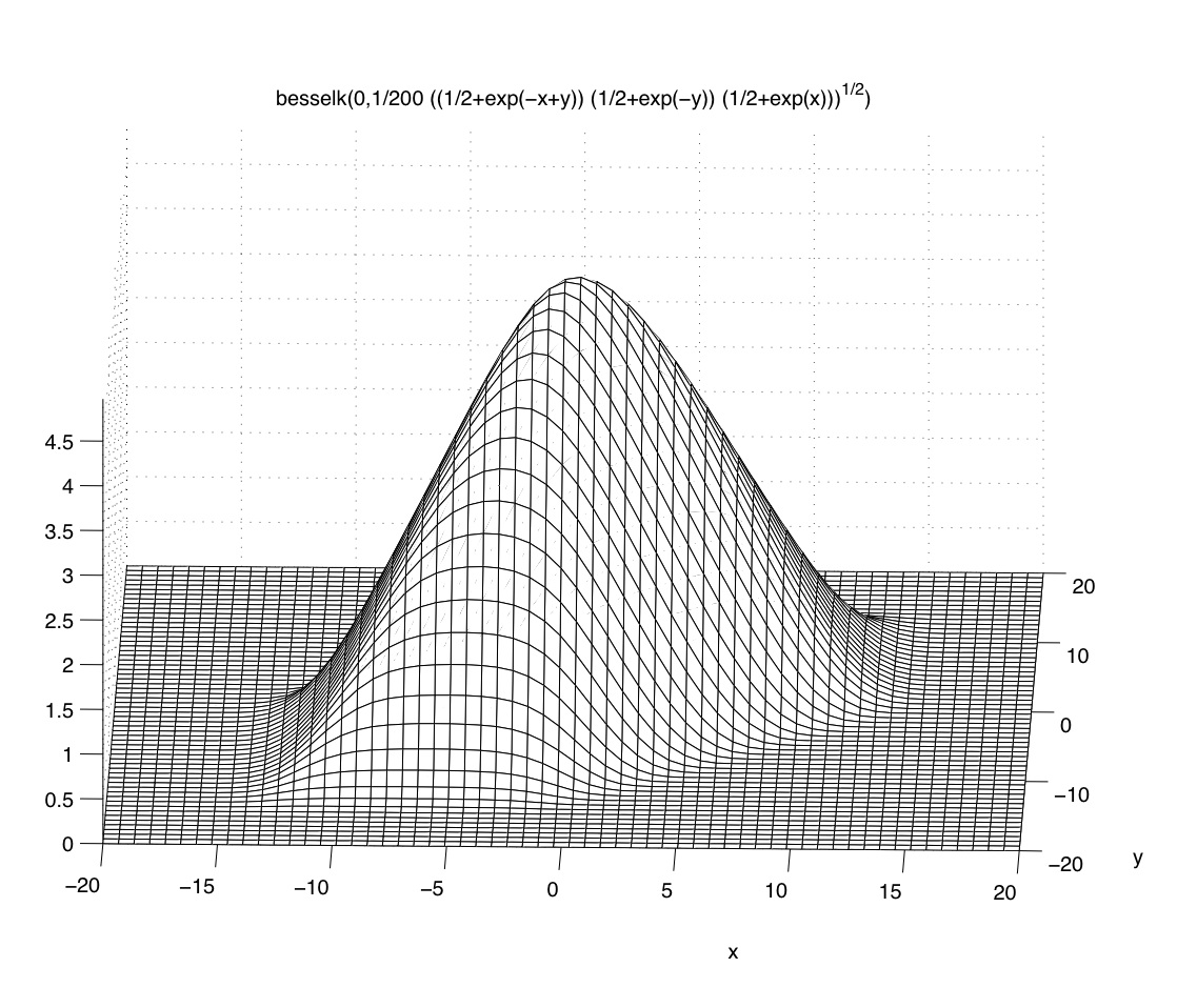
Figure 1: The intertwining kernel $\Lambda(x,\cdot)$

6.2 Behaviour at $-\infty$

From the asymptotic expansion of [7], for any $\lambda$ we have $k_{\mu}(x)^{-1}k_{\lambda}(x)\to 1$ as $x\to-\infty$ (in the sense that $\alpha_{1}(x)\to-\infty$ and $\alpha_{2}(x)\to-\infty$). This suggests that the process with generator

$$\mathcal{L}_{\mu}=\frac{1}{2}\Delta+\nabla\log k_{\mu}\cdot\nabla$$

has a unique entrance law starting from $-\infty$, given by

$$p^{\mu}_{t}(dx)=e^{-\frac{1}{2}\|\mu\|^{2}t}k_{\mu}(x)\theta_{t}(dx),$$

where, for each $t>0$,

$$\int k_{i\tau}(x)\theta_{t}(dx)=e^{-\frac{1}{2}\|\tau\|^{2}t},\qquad\tau\in\Omega.$$

The existence of this entrance law is established (more generally, for type $A_{n}$) in the paper [23]. It is clear from the proof given there that it should be unique. On the other hand:

Proposition 6.1.

Let $(X_{t}^{x_{0}})_{t\geq 0}$ be the diffusion with generator $\mathcal{L}_{\mu}$ started at $x_{0}$. If $\alpha_{1}(x_{0})\to-\infty$ and $\alpha_{2}(x_{0})\to-\infty$, with $\alpha_{1}(x_{0})-\alpha_{2}(x_{0})\rightarrow\kappa$, then

$$\left(e^{\alpha_{1}(x_{0})}\int_{0}^{+\infty}e^{-2\alpha_{1}(X_{s}^{x_{0}})}ds,e^{\alpha_{2}(x_{0})}\int_{0}^{+\infty}e^{-2\alpha_{2}(X_{s}^{x_{0}})}ds\right)$$

converges in probability to $\left(\varphi(e^{\kappa}),\varphi(e^{-\kappa})\right)$, where

$$\varphi(d)=(1+d^{\frac{2}{3}})-d^{\frac{2}{3}}(1+d^{\frac{2}{3}})^{\frac{1}{2}}+d^{\frac{1}{3}}(1+d^{-\frac{2}{3}})^{\frac{1}{2}}.$$

Proof.

Let $\lambda_{1},\lambda_{2}>0$. We easily compute

$$\mathbb{E}\left(\exp\left(-\lambda_{1}e^{\alpha_{1}(x_{0})}\int_{0}^{+\infty}e^{-2\alpha_{1}(X_{s}^{x_{0}})}ds-\lambda_{2}e^{\alpha_{2}(x_{0})}\int_{0}^{+\infty}e^{-2\alpha_{2}(X_{s}^{x_{0}})}ds\right)\right)$$

$$= \frac{\mathbb{E}\exp\left(-\frac{1}{2}(y_{1}^{2}+2\lambda_{1}y_{1})A^{1}_{\infty}-\frac{1}{2}(y_{2}^{2}+2\lambda_{2}y_{2})A^{2}_{\infty}\right)}{\mathbb{E}\exp\left(-\frac{1}{2}y^{2}_{1}A^{1}_{\infty}-\frac{1}{2}y^{2}_{2}A^{2}_{\infty}\right)}$$

with $y_{1}=2e^{-\alpha_{1}(x_{0})},y_{2}=2e^{-\alpha_{2}(x_{0})}$. But, by Lemma 4.2, if $y_{1},y_{2}\to\infty$ with $y_{2}/y_{1}\to\delta=e^{\kappa}$, then

$$\frac{\mathbb{E}\exp\left(-\frac{1}{2}(y_{1}^{2}+2\lambda_{1}y_{1})A^{1}_{\infty}-\frac{1}{2}(y_{2}^{2}+2\lambda_{2}y_{2})A^{2}_{\infty}\right)}{\mathbb{E}\exp\left(-\frac{1}{2}y^{2}_{1}A^{1}_{\infty}-\frac{1}{2}y^{2}_{2}A^{2}_{\infty}\right)}\to e^{-\lambda_{1}\varphi(\delta)-\lambda_{2}\varphi(1/\delta)}.$$

∎

Acknowledgements. We are grateful to the anonymous referees for helpful suggestions. Research of second author was supported in part by Science Foundation Ireland grant number SFI 04-RP1-I512.

References

- [1] L. Alili, H. Matsumoto and T. Shiraishi. On a triplet of exponential brownian functionals. Séminaire de probabilités de Strasbourg, 35 (2001) 396–415.
- [2] F. Baudoin. Further exponential generalization of Pitman’s theorem. Electron. Comm. Probab. 7 (2002), 37–46 (electronic).
- [3] F. Baudoin. Conditioned stochastic differential equations: Theory, Examples and Applications to finance, Stoch. Proc. Appl., Vol. 100, 1, pp. 109-145, (2002).
- [4] Ph. Biane, Ph. Bougerol and N. O’Connell. Littelmann paths and Brownian paths. Duke Math. J. 130 (2005), no. 1, 127–167.
- [5] Ph. Bougerol and T. Jeulin. Paths in Weyl chambers and random matrices. Probab. Theory Related Fields 124 (2002), no. 4, 517–543.
- [6] D. Bump. Automorphic forms on GL(3,. Lecture Notes in Mathematics, 1083. Springer-Verlag, Berlin, 1984.
- [7] D. Bump and J. Huntley. Unramified Whittaker functions for . J. Anal. Math. 65 (1995) 19-44.
- [8] D. Dufresne. The integral of geometric Brownian motion. Adv. Appl. Prob. 33 (2001) 223 241.
- [9] R. Ghomrasni. On distribution associated with the generalized Levy’s stochastic area formula. StudiaSci. Math. Hungar. Vol. 41, No. 1 (2004), 93-100.
- [10] S.G. Gindikin and F.I. Karpelevich. The Plancherel measure for Riemannian symmetric spaces with non-positive curvature. Dokl. Akad. Nauk USSR 145 (1962) 252–255.
- [11] A. Givental. Stationary phase integrals, quantum Toda lattices, flag manifolds and the mirror conjecture. Topics in Singularity Theory, AMS Transl. Ser. 2, vol. 180, AMS, Rhode Island (1997) 103–115.
- [12] C. Grosche. The path integral on the Poincaré upper half-plane with a magnetic field and for the Morse potential. Ann. Phys. 187, No. 1 (1988) 110-134.
- [13] M. Hashizume. Whittaker functions on semisimple Lie groups. Hiroshima Math. J. 12 (1982), no. 2, 259–293.
- [14] N. Ikeda and H. Matsumoto. Brownian motion on the Hyperbolic plane and Selberg trace formula. J. Func. Anal. 163 (1999), 63-110.
- [15] H. Jacquet. Fonctions de Whittaker associées aux groupes de Chevalley. Bull. Soc. Math. France 95 1967 243–309.
- [16] S. Kharchev and D. Lebedev. Integral representations for the eigenfunctions of a quantum periodic Toda chain. Letters in Mathematical Physics 50 (1999), 53–77.
- [17] B. Kostant. Quantisation and representation theory. In: Representation Theory of Lie Groups, Proc. SRC/LMS Research Symposium, Oxford 1977, LMS Lecture Notes 34, Cambridge University Press, 1977, pp. 287–316.
- [18] N.N. Lebedev. Special Functions and their Applications. Dover, 1972.
- [19] H. Matsumoto and M. Yor. A version of Pitman’s theorem for geometric Brownian motions. C. R. Acad. Sci. Paris 328, Série 1 (1999) 1067–1074.
- [20] H. Matsumoto and M. Yor. Exponential functionals of Brownian motion, I: Probability laws at a fixed time. Probability Surveys 2005, Vol. 2, 312–347.
- [21] H. Matsumoto and M. Yor. A relationship between Brownian motions with opposite drifts. Osaka J. Math. 38 (2001).
- [22] N. O’Connell. Random matrices, non-colliding processes and queues. Séminaire de Probabilités, XXXVI, 165–182, Lecture Notes in Math., 1801, Springer, Berlin, 2003.
- [23] N. O’Connell. Directed polymers and the quantum Toda lattice. arXiv:0910.0069
- [24] N. O’Connell and M. Yor. Brownian analogues of Burke’s theorem. Stochastic Process. Appl. 96 (2001) 285–304.
- [25] N. O’Connell and M. Yor. A representation for non-colliding random walks. Elect. Commun. Probab. 7 (2002) 1-12.
- [26] J.W. Pitman. One-dimensional Brownian motion and the three-dimensional Bessel process, Adv. Appl. Probab. 7 (1975) 511-526.
- [27] L. C. G. Rogers and J. Pitman. Markov functions. Ann. Probab. 9 (1981) 573–582.
- [28] M. Semenov-Tian-Shansky. Quantisation of open Toda lattices. In: Dynamical systems VII: Integrable systems, nonholonomic dynamical systems. Edited by V. I. Arnol’d and S. P. Novikov. Encyclopaedia of Mathematical Sciences, 16. Springer-Verlag, Berlin, 1994, pp. 226–259.
- [29] E. Stade. Poincaré series for -Whittaker functions. Duke Math. J. 58 (1989) 695–729.
- [30] A. Vinogradov and L. Takhtadzhyan. Theory of Eisenstein series for the group and its application to a binary problem. J. Soviet Math. 18 (1982) 293–324.