Global Properties of Nucleus-Nucleus Collisions

1 Introduction

QCD as a theory of extended, strongly interacting matter is familiar from big bang evolution which, within the time interval from electro-weak decoupling ($10^{-12}$ s) to hadron formation ($5\cdot 10^{-6}$ s), is dominated by the expansion of quark-gluon matter, a color conducting plasma that is deconfined. In the 1970’s deconfinement was predicted 36 ; 2 ; 37 to arise from the newly discovered “asymptotic freedom” property of QCD; i.e. the plasma was expected to be a solution of perturbative QCD at asymptotically high square-momentum transfer $Q^{2}$, or temperature $T$. Thus the Quark-Gluon-Plasma (QGP) was seen as a dilute gas of weakly coupled partons. This picture may well hold true at temperatures in the GeV to TeV range. However it was also known since R. Hagedorns work 38 that hadronic matter features a phase boundary at a very much lower temperature, $T(H)=170$ MeV. As it was tempting to identify this temperature with that of the cosmological hadronization transition, thus suggesting $T(H)=T(\mathrm{crit})$, the QGP state must extend downward to such a low temperature, with $Q^{2}<<1\mathrm{GeV}^{2}$, and far into the non-perturbative sector of QCD, and very far from asymptotic freedom. The fact that, therefore, the confinement-deconfinement physics of QCD, occuring at the parton-hadron phase boundary, had to be explained in terms other than a dilute perturbative parton gas, was largely ignored until rather recently, when laboratory experiments concerning of the QGP had reached maturity.

In order to recreate matter at the corresponding high energy density in the terrestial laboratory one collides heavy nuclei (also called “heavy ions”) at ultrarelativistic energies. Quantum Chromodynamics predicts 2 ; 3 ; 4 a phase transformation to occur between deconfined quarks and confined hadrons. At near-zero net baryon density (corresponding to big bang conditions) non-perturbative Lattice-QCD places this transition at an energy density of about $1\>GeV/fm^{3}$, and at a critical temperature, $T_{crit}$ $\approx$ $170\>MeV$ 4 ; 5 ; 6 ; 7 ; 8 . The ultimate goal of the physics with ultrarelativistic heavy ions is to locate this transition, elaborate its properties, and gain insight into the detailed nature of the deconfined QGP phase that should exist above. What is meant by the term ”ultrarelativistic” is defined by the requirement that the reaction dynamics reaches or exceeds the critical density $\epsilon\approx 1\>GeV/fm^{3}$. Required beam energies turn out 8 to be $\sqrt{s}\geq 10\>GeV$, and various experimental programs have been carried out or are being prepared at the CERN SPS (up to about $20\>GeV$), at the BNL RHIC collider (up to $200\>GeV)$ and finally reaching up to $5.5\>TeV$ at the LHC of CERN.

QCD confinement-deconfinement is of course not limited to the domain that is relevant to cosmological expansion dynamics, at very small excess of baryon over anti-baryon number density and, thus, near zero baryo-chemical potential $\mu_{B}$. In fact, modern QCD suggests 9 ; 10 ; 11 a detailed phase diagram of QCD matter and its states, in the plane of $T$ and baryo-chemical potential $\mu_{B}$. For a map of the QCD matter phase diagram we are thus employing the terminology of the grand canonical Gibbs ensemble that describes an extended volume $V$ of partonic or hadronic matter at temperature $T$. In it, total particle number is not conserved at relativistic energy, due to particle production-annihilation processes occurring at the microscopic level. However, the probability distributions (partition functions) describing the particle species abundances have to respect the presence of certain, to be conserved net quantum numbers ($i$), notably non-zero net baryon number and zero net strangeness and charm. Their global conservation is achieved by a thermodynamic trick, adding to the system Lagrangian a so-called Lagrange multiplier term, for each of such quantum number conservation tasks. This procedure enters a ”chemical potential” $\mu_{i}$ that modifies the partition function via an extra term $\exp{\left(-\mu_{i}/T\right)}$ occuring in the phase space integral (see section 4 for detail). It modifies the canonical ”punishment factor” $\exp{\left(-E/T\right)}$, where $E$ is the total particle energy in vacuum, to arrive at an analogous grand canonical factor for the extended medium,of $\exp{\left(-E/T-\mu_{i}/T\right)}$. This concept is of prime importance for a description of the state of matter created in heavy ion collisions, where net-baryon number (valence quarks) carrying objects are considered — extended ”fireballs” of QCD matter. The same applies to the matter in the interior of neutron stars. The corresponding conservation of net baryon number is introduced into the grand canonical statistical model of QCD matter via the ”baryo-chemical potential” $\mu_{B}$.

We employ this terminology to draw a phase diagram of QCD matter in figure 1, in the variables $T$ and $\mu_{B}$. Note that $\mu_{B}$ is high at low energies of collisions creating a matter fireball. In a head-on collision of two mass 200 nuclei at $\sqrt{s}=15GeV$ the fireball contains about equal numbers of newly created quark-antiquark pairs (of zero net baryon number), and of initial valence quarks. The accomodation of the latter, into created hadronic species, thus requires a formidable redistribution task of net baryon number, reflecting in a high value of $\mu_{B}$. Conversely, at LHC energy ($\sqrt{s}$=5.5TeV in Pb+Pb collisions), the initial valence quarks constitute a mere 5% fraction of the total quark density, correspondingly requiring a small value of $\mu_{B}$. In the extreme, big bang matter evolves toward hadronization (at $T$=170 MeV) featuring a quark over antiquark density excess of $10^{-9}$ only, resulting in $\mu_{B}\approx 0$.

Note that the limits of existence of the hadronic phase are not only reached by temperature increase, to the so-called Hagedorn value $T_{H}$ (which coincides with $T_{crit}$ at $\mu_{B}\rightarrow 0$), but also by density increase to $\varrho>(5-10)\>\varrho_{0}$: ”cold compression” beyond the nuclear matter ground state baryon density $\varrho_{0}$ of about 0.16 $B/fm^{3}$. We are talking about the deep interior sections of neutron stars or about neutron star mergers 12 ; 13 ; 14 . A sketch of the present view of the QCD phase diagram 9 ; 10 ; 11 is given in Fig. 1. It is dominated by the parton-hadron phase transition line that interpolates smoothly between the extremes of predominant matter heating (high $T$, low $\mu_{B}$) and predominant matter compression ($T\rightarrow 0,\>\mu_{B}>1\>GeV$). Onward from the latter conditions, the transition is expected to be of first order 15 until the critical point of QCD matter is reached at $200\leq\mu_{B}\>(E)\>\leq 500\>MeV$. The relatively large position uncertainty reflects the preliminary character of Lattice QCD calculations at finite $\mu_{B}$ 9 ; 10 ; 11 . Onward from the critical point, E, the phase transformation at lower $\mu_{B}$ is a cross-over11 .

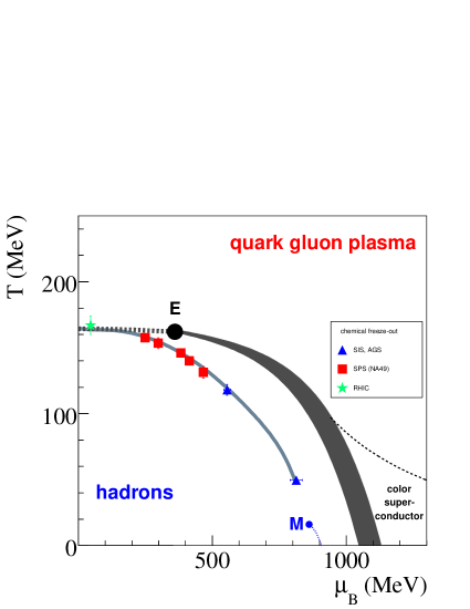
Figure 1: Sketch of the QCD matter phase diagram in the plane of temperature $T$ and baryo-chemical potential $\mu_{B}$. The parton-hadron phase transition line from lattice QCD 8 ; 9 ; 10 ; 11 ends in a critical point $E$. A cross-over transition occurs at smaller $\mu_{B}$. Also shown are the points of hadro-chemical freeze-out from the grand canonical statistical model.

We note, however, that these estimates represent a major recent advance of QCD lattice theory which was, for two decades, believed to be restricted to the $\mu_{B}=0$ situation. Onward from the critical point, toward lower $\mu_{B}$, the phase transformation should acquire the properties of a rapid cross-over 16 , thus also including the case of primordial cosmological expansion. This would finally rule out former ideas, based on the picture of a violent first order ”explosive” cosmological hadronization phase transition, that might have caused non-homogeneous conditions, prevailing during early nucleo-synthesis 17 , and fluctuations of global matter distribution density that could have served as seedlings of galactic cluster formation 18 . However, it needs to be stressed that the conjectured order of phase transformation, occuring along the parton - hadron phase boundary line, has not been unambiguously confirmed by experiment, as of now.

On the other hand, the position of the QCD phase boundary at low $\mu_{B}$ has, in fact, been located by the hadronization points in the $T,\>\mu_{B}$ plane that are also illustrated in Fig. 1. They are obtained from statistical model analysis 19 of the various hadron multiplicities created in nucleus-nucleus collisions, which results in a [$T,\>\mu_{B}$] determination at each incident energy, which ranges from SIS via AGS and SPS to RHIC energies, i.e. $3\leq\sqrt{s}\leq 200\>GeV$. Toward low $\mu_{B}$ these hadronic freeze-out points merge with the lattice QCD parton-hadron coexistence line: hadron formation coincides with hadronic species freeze-out. These points also indicate the $\mu_{B}$ domain of the phase diagram which is accessible to relativistic nuclear collisions. The domain at $\mu_{B}\geq 1.5\>GeV$ which is predicted to be in a further new phase of QCD featuring color-flavor locking and color superconductivity 20 will probably be accessible only to astrophysical observation.

One may wonder how states and phases of matter in thermodynamical equilibrium - as implied by a description in grand canonical variables - can be sampled via the dynamical evolution of relativistic nuclear collisions. Employing heavy nuclei, $A\approx 200$, as projectiles/targets or in colliding beams (RHIC, LHC), transverse dimensions of the primordial interaction volume do not exceed about $8\>fm$, and strong interaction ceases after about $20\>fm/c$. We note, for now, that the time and dimension scale of primordial perturbative QCD interaction at the microscopic partonic level amounts to subfractions of $1\>fm/c$, the latter scale, however, being representative of non perturbative processes (confinement, ”string” formation etc.). The A+A fireball size thus exceeds, by far, the elementary non perturbative scale. An equilibrium quark gluon plasma represents an extended non-perturbative QCD object, and the question whether its relaxation time scale can be provided by the expansion time scale of an A+A collision, needs careful examination. Reassuringly, however, the hadrons that are supposedly created from such a preceding non-perturbative QGP phase at top SPS and RHIC energy, do in fact exhibit perfect hydrodynamic and hadrochemical equilibrium, the derived [$T,\>\mu_{B}$] values 19 thus legitimately appearing in the phase diagram, Fig. 1.

In the present book we will order the physics observables to be treated, with regard to their origin from successive stages that characterize the overall dynamical evolution of a relativistic nucleus-nucleus collision. In rough outline this evolution can be seen to proceed in three major steps. An initial period of matter compression and heating occurs in the course of interpenetration of the projectile and target baryon density distributions. Inelastic processes occuring at the microscopic level convert initial beam longitudinal energy to new internal and transverse degrees of freedom, by breaking up the initial baryon structure functions. Their partons thus acquire virtual mass, populating transverse phase space in the course of inelastic perturbative QCD shower multiplication. This stage should be far from thermal equilibrium, initially. However, in step two, inelastic interaction between the two arising parton fields (opposing each other in longitudinal phase space) should lead to a pile-up of partonic energy density centered at mid-rapidity (the longitudinal coordinate of the overall center of mass). Due to this mutual stopping down of the initial target and projectile parton fragmentation showers, and from the concurrent decrease of parton virtuality (with decreasing average square momentum transfer $Q^{2}$) there results a slowdown of the time scales governing the dynamical evolution. Equilibrium could be approached here, the system ”lands” on the $T,\>\mu$ plane of Fig. 1, at temperatures of about 300 and $200\>MeV$ at top RHIC and top SPS energy, respectively. The third step, system expansion and decay, thus occurs from well above the QCD parton-hadron boundary line. Hadrons and hadronic resonances then form, which decouple swiftly from further inelastic transmutation so that their yield ratios become stationary (”frozen-out”). A final expansion period dilutes the system to a degree such that strong interaction ceases all together.

It is important to note that the above description, in terms of successive global stages of evolution, is only valid at very high energy, e.g. at and above top RHIC energy of $\sqrt{s}=200$GeV. At this energy the target-projectile interpenetration time $2R/\gamma=0.12\mathrm{fm}/c$, and thus the interpenetration phase is over when the supposed next phase (perturbative QCD shower formation at the partonic level by primordial, ”hard” parton scattering) settles, at about $0.25\mathrm{fm}/c$. ”Hard” observables (heavy flavour production, jets, high $p_{T}$ hadrons) all originate from this primordial interaction phase. On the other hand it is important to realize that at top SPS energy, $\sqrt{s}=17.3$GeV, global interpenetration takes as long as 1.5fm/$c$, much longer than microscopic shower formation time. There is thus no global, distinguishable phase of hard QCD mechanisms: they are convoluted with the much longer interpenetration time. During that it is thus impossible to consider a global physics of the interaction volume, or any equilibrium. Thus we can think of the dynamical evolution in terms of global ”states” of the system’s dynamical evolution (such as local or global equilibrium) only after about 2-3fm/$c$, just before bulk hadronization sets in. Whereas at RHIC, and even more ideally so at the LHC, the total interaction volume is ”synchronized” at times below 0.5fm/$c$, such that a hydrodynamic description becomes possible: we can expect that ”flow” of partons sets in at this time, characterized by extremely high parton density. The dynamics at such early time can thus be accessed in well defined variables (e.g. elliptic flow or jet quenching).

In order to verify in detail this qualitative overall model, and to ascertain the existence (and to study the properties) of the different states of QCD that are populated in sequence, one seeks observable physics quantities that convey information imprinted during distinct stages of the dynamical evolution, and ”freezing-out” without significant obliteration by subsequent stages. Ordered in sequence of their formation in the course of the dynamics, the most relevant such observables are briefly characterized below:

1. Suppression of $J/\Psi$ and $Y$ production by Debye-screening in the QGP. These vector mesons result from primordial, pQCD production of $c\overline{c}$ and $b\overline{b}$ pairs that would hadronize unimpeded in elementary collisions but are broken up if immersed into a npQCD deconfined QGP, at certain characteristic temperature thresholds.

2. Suppression of dijets which arise from primordial $q\overline{q}$ pair production fragmenting into partonic showers (jets) in vacuum but being attenuated by QGP-medium induced gluonic bremsstrahlung: Jet quenching in A+A collisions.

   1. A variant of this: any primordial hard parton suffers a high, specific loss of energy when traversing a deconfined medium: High $p_{T}$ suppression in A+A collisions.

3. Hydrodynamic collective motion develops with the onset of (local) thermal equilibrium. It is created by partonic pressure gradients that reflect the initial collisional impact geometry via non-isotropies in particle emission called ”directed” and ”elliptic” flow. The latter reveals properties of the QGP, seen here as an ideal partonic fluid.

   1. Radial hydrodynamical expansion flow (”Hubble expansion”) is a variant of the above that occurs in central, head on collisions with cylinder symmetry, as a consequence of an isentropic expansion. It should be sensitive to the mixed phase conditions characteristic of a first order parton-hadron phase transition.

4. Hadronic ”chemical” freeze-out fixes the abundance ratios of the hadronic species into an equilibrium distribution. Occuring very close to, or at hadronization, it reveals the dynamical evolution path in the [$T,\>\mu_{B}$] plane and determines the critical temperature and density of QCD. The yield distributions in A+A collisions show a dramatic strangeness enhancement effect, characteristic of an extended QCD medium.

5. Fluctuations, from one collision event to another (and even within a single given event) can be quantified in A+A collisions due to the high charged hadron multiplicity density (of up to 600 per rapidity unit at top RHIC energy). Such event-by-event (ebye) fluctuations of pion rapidity density and mean transverse momentum (event ”temperature”), as well as event-wise fluctuations of the strange to non-strange hadron abundance ratio (may) reflect the existence and position of the conjectured critical point of QCD (Fig. 1).

6. Two particle Bose-Einstein-Correlations are the analog of the Hanbury-Brown, Twiss (HBT) effect of quantum optics. They result from the last interaction experienced by mesons, i.e. from the global decoupling stage. Owing to a near isentropic hadronic expansion they reveal information on the overall space-time-development of the ”fireball” evolution.

In an overall view the first group of observables (1 to 2a) is anchored in established pQCD physics that is well known from theoretical and experimental analysis of elementary collisions ($e^{+}e^{-}$ annihilation, $pp$ and $p\overline{p}$ data). In fact, the first generation of high $Q^{2}$ baryon collisions, occuring at the microscopic level in A+A collisions, should closely resemble such processes. However, their primary partonic products do not escape into pQCD vacuum but get attenuated by interaction with the concurrently developing extended high density medium , thus serving as diagnostic tracer probes of that state. The remaining observables capture snapshots of the bulk matter medium itself. After initial equilibration we may confront elliptic flow data with QCD during the corresponding partonic phase of the dynamical evolution employing thermodynamic 21 and hydrodynamic 22 models of a high temperature parton plasma. The hydro-model stays applicable well into the hadronic phase. Hadron formation (confinement) occurs in between these phases (at about 5 microseconds time in the cosmological evolution). In fact relativistic nuclear collision data may help to finally pin down the mechanism(s) of this fascinating QCD process 23 ; 24 ; 25 as we can vary the conditions of its occurence, along the parton-hadron phase separation line of Fig. 1, by proper choice of collisional energy $\sqrt{s}$, and system size A, while maintaining the overall conditions of an extended imbedding medium of high energy density within which various patterns 9 ; 10 ; 11 ; 15 ; 16 of the hadronization phase transition may establish. The remaining physics observables (3a, 5 and 6 above) essentially provide for auxiliary information about the bulk matter system as it traverses (and emerges from) the hadronization stage, with special emphasis placed on manifestations of the conjectured critical point.

The observables from 1 to 4 above will all be treated, in detail, in this book. We shall focus here on the bulk matter expansion processes of the primordially formed collisional volume, as reflected globally in the population patterns of transverse and longitudinal (rapidity) phase space (Section 3), and on the transition from partons to hadrons and on hadronic hadro-chemical decoupling, resulting in the observed abundance systematics of the hadronic species (Section 4).These Sections will be preceded by a detailed recapitulation of relativistic kinematics, notably rapidity, to which we shall turn now.

2 Relativistic Kinematics

2.1 Description of Nucleus-Nucleus Collisions in terms of Light-Cone Variables

In relativistic nucleus-nucleus collisions, it is convenient to use kinematic variables which take simple forms under Lorentz transformations for the change of frame of reference. A few of them are the light cone variables $x_{+}$ and $x_{-}$, the rapidity and pseudorapidity variables, $y$ and $\eta$. A particle is characterized by its 4-momentum, $p_{\mu}=(E,{\bf p})$. In fixed target and collider experiments where the beam(s) define reference frames, boosted along their direction, it is important to express the 4-momentum in terms of more practical kinematic variables.

Figure 2 shows the collision of two Lorentz contracted nuclei approaching each other with velocities nearly equal to velocity of light. The vertical axis represents the time direction with the lower half representing time before the collision and the upper half, time after the collision. The horizontal axis represents the spatial direction. Both the nuclei collide at $(t,z)=(0,0)$ and then the created fireball expands in time going through various processes till the created particles freeze-out and reach the detectors. The lines where $t^{2}-z^{2}~{}=~{}0$ (note that $\sqrt{t^{2}-z^{2}}~{}\equiv~{}\tau$, $\tau$ being the proper time of the particle) along the path of the colliding nuclei define the light cone. The upper part of the light-cone, where $t^{2}-z^{2}~{}>~{}0$, is the time-like region. In nucleus-nucleus collisions, particle production occurs in the upper half of the $(t,z)$-plane within the light-cone. The region outside the light cone for which $t^{2}-z^{2}~{}<~{}0$ is called space-like region. The space-time rapidity is defined as

$$\eta_{s}~{}=~{}\frac{1}{2}~{}ln\left(\frac{t+z}{t-z}\right)$$ (1)

It could be seen that $\eta_{s}$ is not defined in the space-like region. It takes the value of positive and negative infinity along the beam directions for which $t=\pm z$ respectively. A particle is ”light-like” along the beam direction. Inside the light-cone which is time-like, $\eta_{s}$ is properly defined.

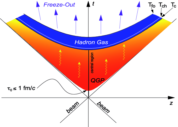
Figure 2: Description of heavy-ion collisions in one space ($z$) and one time ($t$) dimension.

For a particle with 4-momentum $p~{}(p_{0},{\bf p_{T}},p_{z})$, the light-cone momenta are defined by

$$p_{+} = p_{0}+p_{z}$$ (2)

$$p_{-} = p_{0}-p_{z}$$ (3)

$p_{+}$ is called “forward light-cone momentum” and $p_{-}$ is called “backward light-cone momentum”.
For a particle traveling along the beam direction, has higher value of forward light-cone momentum and traveling opposite to the beam direction has lower value of forward light-cone momentum. The advantages of using light-cone variables to study particle production are the following.
1. The forward light-cone momentum of any particle in one frame is related to the forward light-cone momentum of the same particle in another boosted Lorentz frame by a constant factor.
2. Hence, if a daughter particle $c$ is fragmenting from a parent particle $b$, then the ratio of the forward light-cone momentum of $c$ relative to that of $b$ is independent of the Lorentz frame.
Define

$$x_{+} = \frac{p_{0}^{c}+p_{z}^{c}}{p_{0}^{b}+p_{z}^{b}}$$

$$= \frac{c_{+}}{b_{+}}.$$

The forward light-cone variable $x_{+}$ is always positive because $c_{+}$ can’t be greater than $b_{+}$. Hence the upper limit of $x_{+}$ is $1$. $x_{+}$ is Lorentz invariant.
3. The Lorentz invariance of $x_{+}$ provides a tool to measure the momentum of any particle in the scale of the momentum of any reference particle.

2.2 The Rapidity Variable

The co-ordinates along the beam line (conventionally along the $z$-axis) is called longitudinal and perpendicular to it is called transverse (x-y). The 3-momentum can be decomposed into the longitudinal ($p_{z}$) and the transverse (${\bf p}_{T})$, ${\bf p}_{T}$ being a vector quantity which is invariant under a Lorentz boost along the longitudinal direction. The variable rapidity “$y$” is defined by

$$y=\frac{1}{2}ln\left(\frac{E+p_{z}}{E-p_{z}}\right).$$ (5)

It is a dimensionless quantity related to the ratio of forward light-cone to backward light-cone momentum. The rapidity changes by an additive constant under longitudinal Lorentz boosts.

For a free particle which is on the mass shell (for which $E^{2}=p^{2}+m^{2}$), the 4-momentum has only three degrees of freedom and can be represented by $(y,{\bf p}_{T})$. $(E,{\bf p}_{T})$ could be expressed in terms of $(y,{\bf p}_{T})$ as

$$E = m_{T}~{}cosh~{}y$$ (6)

$$p_{z} = m_{T}~{}sinh~{}y$$ (7)

$m_{T}$ being the transverse mass which is defined as

$$m_{T}^{2}=m^{2}+{\bf p}_{T}^{2}.$$ (8)

The advantage of rapidity variable is that the shape of the rapidity distribution remains unchanged under a longitudinal Lorentz boost. When we go from CMS to LS, the rapidity distribution is the same, with the $y$-scale shifted by an amount equal to $y_{cm}$. This is shown below.

Rapidity of Center of Mass in the Laboratory System

The total energy in the CMS system is $E_{cm}=\sqrt{s}$. The energy and momentum of the CMS in the LS are $\gamma_{cm}\sqrt{s}$ and $\beta_{cm}\gamma_{cm}\sqrt{s}$ respectively. The rapidity of the CMS in the LS is

$$y_{cm} = \frac{1}{2}~{}ln\left[\frac{\gamma_{cm}\sqrt{s}+\beta_{cm}\gamma_{cm}\sqrt{s}}{\gamma_{cm}\sqrt{s}-\beta_{cm}\gamma_{cm}\sqrt{s}}\right]$$ (9)

$$= \frac{1}{2}~{}ln\left[\frac{1+\beta_{cm}}{1-\beta_{cm}}\right]$$

It is a constant for a particular Lorentz transformation.

Relationship between Rapidity of a particle in LS and rapidity in CMS

The rapidities of a particle in the LS and CMS of the collision are respectively, $y=\frac{1}{2}~{}ln\left(\frac{E+p_{z}}{E-p_{z}}\right)$ and $y^{*}=\frac{1}{2}~{}ln\left(\frac{E^{*}+p_{z}^{*}}{E^{*}-p_{z}^{*}}\right)$. Inverse Lorentz transformations on $E$ and $p_{z}$ give

$$y = \frac{1}{2}~{}ln\left[\frac{\gamma(E^{*}+\beta p_{z}^{*})+\gamma(\beta E^{*}+p_{z}^{*})}{\gamma(E^{*}+\beta p_{z}^{*})-\gamma(\beta E^{*}+p_{z}^{*})}\right]$$ (10)

$$= \frac{1}{2}~{}ln\left[\frac{E^{*}+p_{z}^{*}}{E^{*}-p_{z}^{*}}\right]+\frac{1}{2}~{}ln\left[\frac{1+\beta}{1-\beta}\right]$$

$$\Rightarrow y = y^{*}+y_{cm}.$$ (11)

Hence the rapidity of a particle in the laboratory system is equal to the sum of the rapidity of the particle in the center of mass system and the rapidity of the center of mass in the laboratory system. It can also be state that the rapidity of a particle in a moving (boosted) frame is equal to the rapidity in its own rest frame minus the rapidity of the moving frame. In the non-relativistic limit, this is like the subtraction of velocity of the moving frame. However, this is not surprising because, non-relativistically, the rapidity $y$ is equal to longitudinal velocity $\beta$. Rapidity is a relativistic measure of the velocity. This simple property of the rapidity variable under Lorentz transformation makes it a suitable choice to describe the dynamics of relativistic particles.

Relationship between Rapidity and Velocity

Consider a particle traveling in $z$-direction with a longitudinal velocity $\beta$. The energy $E$ and the longitudinal momentum $p_{z}$ of the particle are

$$E = \gamma m$$ (12)

$$p_{z} = \gamma\beta m$$ (13)

where $m$ is the rest mass of the particle. Hence the rapidity of the particle traveling in $z$-direction with velocity $\beta$ is

$$y_{\beta} = \frac{1}{2}~{}ln\left[\frac{E+p_{z}}{E-p_{z}}\right]=\frac{1}{2}~{}ln\left[\frac{\gamma m+\gamma\beta m}{\gamma m-\gamma\beta m}\right]$$ (14)

$$= \frac{1}{2}~{}ln\left[\frac{1+\beta}{1-\beta}\right]$$

Note here that $y_{\beta}$ is independent of particle mass. In the non-relativistic limit when $\beta$ is small, expanding $y_{\beta}$ in terms of $\beta$ leads to

$$y_{\beta}=\beta+{\it O}(\beta^{3})$$ (15)

Thus the rapidity of the particle is the relativistic realization of its velocity.

Beam Rapidity

We know,
$E~{}=~{}m_{T}~{}cosh~{}y$, $p_{z}~{}=~{}m_{T}~{}sinh~{}y$ and $m_{T}^{2}=m^{2}+{\bf p}_{T}^{2}$.
For the beam particles, $p_{T}=0$.
Hence, $E~{}=~{}m_{b}~{}cosh~{}y_{b}$ and $p_{z}~{}=~{}m_{b}~{}sinh~{}y_{b}$,
where $m_{b}$ and $y_{b}$ are the rest mass and rapidity of the beam particles.

$$y_{b} = cosh^{-1}~{}(E/m_{b})$$ (16)

$$= cosh^{-1}~{}\left[\frac{\sqrt{s_{NN}}}{2~{}m_{n}}\right]$$

and

$$y_{b}=sinh^{-1}~{}(p_{z}/m_{b})$$ (17)

Here $m_{n}$ is the mass of the nucleon. Note that the beam energy $E=\sqrt{s_{NN}}/2$.

Example 1

For the nucleon-nucleon center of mass energy $\sqrt{s_{NN}}=9.1$ GeV, the beam rapidity $y_{b}~{}=~{}cosh^{-1}\left(\frac{9.1}{2\times 0.938}\right)~{}=~{}2.26$
For p+p collisions with lab momentum 100 GeV/c,
$y_{b}~{}=~{}sinh^{-1}\left(\frac{p_{z}}{m_{b}}\right)~{}=~{}sinh^{-1}\left(\frac{100}{0.938}\right)~{}=~{}5.36$
and for Pb+Pb collisions at SPS with lab energy 158 AGeV, $y_{b}~{}=~{}2.92$.

Rapidity of the CMS in terms of Projectile and Target Rapidities

Let us consider the beam particle “$b$” and the target particle “$a$”.
$b_{z}~{}=~{}m_{T}~{}sinh~{}y_{b}~{}=~{}m_{b}~{}sinh~{}y_{b}$. This is because $p_{T}$ of beam particles is zero. Hence

$$y_{b}~{}=~{}sinh^{-1}~{}(b_{z}/m_{b}).$$ (18)

The energy of the beam particle in the laboratory frame is
$b_{0}~{}=~{}m_{T}~{}cosh~{}y_{b}~{}=~{}m_{b}~{}cosh~{}y_{b}$.
Assuming target particle $a$ has longitudinal momentum $a_{z}$, its rapidity in the laboratory frame is given by

$$y_{a}~{}=~{}sinh^{-1}~{}(a_{z}/m_{a})$$ (19)

and its energy

$$a_{0}~{}=~{}m_{a}~{}cosh~{}y_{a}.$$ (20)

The CMS is obtained by boosting the LS by a velocity of the center-of-mass frame $\beta_{cm}$ such that the longitudinal momentum of the beam particle $b_{z}^{*}$ and of the target particle $a_{z}^{*}$ are equal and opposite. Hence $\beta_{cm}$ satisfies the condition,
$a_{z}^{*}~{}=~{}\gamma_{cm}(a_{z}-\beta_{cm}a_{0})~{}=~{}-b_{z}^{*}~{}=~{}-\gamma_{cm}(b_{z}-\beta_{cm}b_{0})$, where $\gamma_{cm}~{}=~{}\frac{1}{\sqrt{1-\beta_{cm}^{2}}}$. Hence,

$$\beta_{cm}~{}=~{}\frac{a_{z}+b_{z}}{a_{0}+b_{0}}.$$ (21)

We know the rapidity of the center of mass is

$$y_{cm}~{}=~{}\frac{1}{2}~{}ln\left[\frac{1+\beta_{cm}}{1-\beta_{cm}}\right]$$ (22)

Using equations 21 and 22, we get

$$y_{cm}~{}=~{}\frac{1}{2}~{}ln\left[\frac{a_{0}+a_{z}+b_{0}+b_{z}}{a_{0}-a_{z}+b_{0}-b_{z}}\right].$$ (23)

Writing energies and momenta in terms of rapidity variables in the LS,

$$y_{cm} = \frac{1}{2}~{}ln\left[\frac{m_{a}~{}cosh~{}y_{a}+m_{a}~{}sinh~{}y_{a}+m_{b}~{}cosh~{}y_{b}+m_{b}~{}sinh~{}y_{b}}{m_{a}~{}cosh~{}y_{a}-m_{a}~{}sinh~{}y_{a}+m_{b}~{}cosh~{}y_{b}-m_{b}~{}sinh~{}y_{b}}\right]$$ (24)

$$= \frac{1}{2}(y_{a}+y_{b})~{}+~{}\frac{1}{2}~{}ln\left[\frac{m_{a}~{}e^{y_{a}}+m_{b}~{}e^{y_{b}}}{m_{a}~{}e^{y_{b}}+m_{b}~{}e^{y_{a}}}\right]$$

For a symmetric collision (for $m_{a}~{}=~{}m_{b}$),

$$y_{cm}~{}=~{}\frac{1}{2}(y_{a}+y_{b})$$ (25)

Rapidities of $a$ and $b$ in the CMS are

$$y_{a}^{*}~{}=~{}y_{a}-y_{cm}~{}=~{}-\frac{1}{2}(y_{b}-y_{a})$$ (26)

$$y_{b}^{*}~{}=~{}y_{b}-y_{cm}~{}=~{}\frac{1}{2}(y_{b}-y_{a}).$$ (27)

Given the incident energy, the rapidity of projectile particles and the rapidity of the target particles can thus be determined. The greater is the incident energy, the greater is the separation between the projectile and target rapidity.

Central Rapidity

The region of rapidity mid-way between the projectile and target rapidities is called central rapidity.

Example 2

In p+p collisions at a laboratory momentum of 100 $GeV/c$, beam rapidity $y_{b}=5.36$, target rapidity $y_{a}=0$ and the central rapidity $\approx 2.7$.

Mid-rapidity in Fixed target and Collider Experiments

In fixed-target experiments (LS), $y_{target}~{}=~{}0$.
$y_{lab}~{}=~{}y_{target}~{}+~{}y_{projectile}~{}=~{}y_{beam}$ Hence mid-rapidity in fixed-target experiment is given by,

$$y_{mid}^{LS}~{}=~{}y_{beam}/2.$$ (28)

In collider experiments (center of mass system),
$y_{projectile}~{}=~{}-y_{target}~{}=~{}y_{CMS}~{}=~{}y_{beam}/2$.
Hence, mid-rapidity in CMS system is given by

$$y_{mid}^{CMS}~{}=~{}(y_{projectile}+y_{target})/2~{}=~{}0.$$ (29)

This is valid for a symmetric energy collider. The rapidity difference is given by $y_{projectile}-y_{target}=2y_{CMS}$ and this increases with energy for a collider as $y$ increases with energy.

Light-cone variables and Rapidity

Consider a particle having rapidity $y$ and the beam rapidity is $y_{b}$. The particle has forward light-cone variable $x_{+}$ with respect to the beam particle

$$x_{+} = \frac{p_{0}^{c}+p_{z}^{c}}{p_{0}^{b}+p_{z}^{b}}$$ (30)

$$= \frac{m_{T}^{c}}{m^{b}}e^{y-y_{b}}$$

where $m_{T}^{c}$ is the transverse mass of $c$. Note that the transverse momentum of the beam particle is zero. Hence,

$$y = y_{b}+ln~{}x_{+}+ln\left(\frac{m_{b}}{m_{T}^{c}}\right)$$ (31)

Similarly, relative to the target particle $a$ with a target rapidity $y_{a}$, the backward light-cone variable of the detected particle $c$ is $x_{-}$. $x_{-}$ is related to $y$ by

$$x_{-}=\frac{m_{T}^{c}}{m^{b}}e^{y_{a}-y}$$ (32)

and conversely,

$$y=y_{a}-ln~{}x_{-}-ln\left(\frac{m_{a}}{m_{T}^{c}}\right).$$ (33)

In general, the rapidity of a particle is related to its light-cone momenta by

$$y=\frac{1}{2}~{}ln\left(\frac{p_{+}}{p_{-}}\right)$$ (34)

Note that in situations where there is a frequent need to work with boosts along z-direction, it’s better to use $(y,{\bf p_{T}})$ for a particle rather than using it’s 3-momentum, because of the simple transformation rules for $y$ and ${\bf p_{T}}$ under Lorentz boosts.

2.3 The Pseudorapidity Variable

Let us assume that a particle is emitted at an angle $\theta$ relative to the beam axis. Then its rapidity can be written as
$y~{}=~{}\frac{1}{2}~{}ln\left(\frac{E+P_{L}}{E-P_{L}}\right)~{}=~{}\frac{1}{2}~{}ln\left[\frac{\sqrt{m^{2}+p^{2}}+p~{}cos~{}\theta}{\sqrt{m^{2}+p^{2}}-p~{}cos~{}\theta}\right]$. At very high energy, $p\gg m$ and hence

$$y = \frac{1}{2}~{}ln\left[\frac{p+p~{}cos~{}\theta}{p-p~{}cos~{}\theta}\right]$$ (35)

$$= -ln~{}tan~{}\theta/2\equiv\eta$$

$\eta$ is called the pseudorapidity. Hence at very high energy,

$$y~{}\approx~{}\eta~{}=~{}-ln~{}tan~{}\theta/2.$$ (36)

In terms of the momentum, $\eta$ can be re-written as

$$\eta~{}=~{}\frac{1}{2}~{}ln\left[\frac{|{\bf p}|+p_{z}}{|{\bf p}|-p_{z}}\right].$$ (37)

$\theta$ is the only quantity to be measured for the determination of pseudorapidity, independent of any particle identification mechanism. Pseudorapidity is defined for any value of mass, momentum and energy of the collision. This also could be measured with or without momentum information which needs a magnetic field.

Change of variables from $(y,{\bf p}_{T})$ to $(\eta,{\bf p}_{T})$

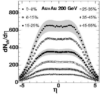
Figure 3: The mid-rapidity $dN_{ch}/d\eta$ for Au+Au collisions at $\sqrt{s_{NN}}=$ 200 GeV phobos .

By equation 37,

$$e^{\eta} = \sqrt{\frac{|{\bf p}|+p_{z}}{|{\bf p}|-p_{z}}}$$ (38)

$$e^{-\eta} = \sqrt{\frac{|{\bf p}|-p_{z}}{|{\bf p}|+p_{z}}}$$ (39)

Adding both of the equations, we get

$$|{\bf p}|~{}=~{}p_{T}~{}cosh~{}\eta$$ (40)

${\bf p}_{T}~{}=~{}\sqrt{|{\bf p}|^{2}-p_{z}^{2}}$. By subtracting the above equations, we get

$$p_{z}~{}=~{}p_{T}~{}sinh~{}\eta$$ (41)

Using these equations in the definition of rapidity, we get

$$y~{}=~{}\frac{1}{2}~{}ln\left[\frac{\sqrt{p_{T}^{2}~{}cosh^{2}~{}\eta+m^{2}}+p_{T}~{}sinh~{}\eta}{\sqrt{p_{T}^{2}~{}cosh^{2}~{}\eta+m^{2}}-p_{T}~{}sinh~{}\eta}\right]$$ (42)

Similarly $\eta$ could be expressed in terms of $y$ as,

$$\eta~{}=~{}\frac{1}{2}~{}ln\left[\frac{\sqrt{m_{T}^{2}~{}cosh^{2}~{}y-m^{2}}+m_{T}~{}sinh~{}y}{\sqrt{m_{T}^{2}~{}cosh^{2}~{}y-m^{2}}-m_{T}~{}sinh~{}y}\right]$$ (43)

The distribution of particles as a function of rapidity is related to the distribution as a function of pseudorapidity by the formula

$$\frac{dN}{d\eta d{\bf p}_{T}}~{}=~{}\sqrt{1-\frac{m^{2}}{m_{T}^{2}~{}cosh^{2}~{}y}}~{}\frac{dN}{dyd{\bf p}_{T}}.$$ (44)

In the region $y\gg 0$, the pseudorapidity distribution ($dN/d\eta$) and the rapidity distribution ($dN/dy$) which are essentially the ${\bf p}_{T}$-integrated values of $\frac{dN}{d\eta d{\bf p}_{T}}$ and $\frac{dN}{dyd{\bf p}_{T}}$ respectively, are approximately the same. In the region $y\approx 0$, there is a small “depression” in $dN/d\eta$ distribution compared to $dN/dy$ distribution due to the above transformation. At very high energies where $dN/dy$ has a mid-rapidity plateau, this transformation gives a small dip in $dN/d\eta$ around $\eta\approx 0$ (see Figure 3). However, for a massless particle like photon, the dip in $dN/d\eta$ is not expected (which is clear from the above equation). Independent of the frame of reference where $\eta$ is measured, the difference in the maximum magnitude of $dN/d\eta$ appears due to the above transformation. In the CMS, the maximum of the distribution is located at $y\approx\eta\approx 0$ and the $\eta$-distribution is suppressed by a factor $\sqrt{1-m^{2}/<m_{T}^{2}>}$ with reference to the rapidity distribution. In the laboratory frame, however the maximum is located around half of the beam rapidity $\eta\approx y_{b}/2$ and the suppression factor is $\sqrt{1-m^{2}/<m_{T}^{2}>~{}cosh^{2}~{}(y_{b}/2)}$, which is about unity. Given the fact that the shape of the rapidity distribution is independent of frame of reference, the peak value of the pseudorapidity distribution in the CMS frame is lower than its value in LS. This suppression factor at SPS energies is $\sim 0.8~{}-~{}0.9$.

2.4 The Invariant Yield

First we show $\frac{d^{3}p}{E}$ is Lorentz invariant. The differential of Lorentz boost in longitudinal direction is given by

$$dp_{z}^{*}~{}=~{}\gamma(dp_{z}-\beta dE).$$ (45)

Taking the derivative of the equation $E^{2}~{}=~{}p^{2}+m^{2}$, we get

$$EdE~{}=~{}p_{z}dp_{z}.$$ (46)

Using equations 45 and 46 we get

$$dp_{z}^{*} = \gamma(dp_{z}-\beta\frac{p_{z}dp_{z}}{E})$$ (47)

$$= \frac{dp_{z}}{E}~{}E^{*}.$$

As ${\bf p}_{T}$ is Lorentz invariant, multiplying ${\bf p}_{T}$ on both the sides and re-arranging gives

$$\frac{d^{3}p^{*}}{E^{*}}~{}=~{}\frac{d^{2}{\bf p}_{T}~{}dp_{z}}{E}~{}=~{}\frac{d^{3}p}{E}.$$ (48)

In terms of experimentally measurable quantities, $\frac{d^{3}p}{E}$ could be expressed as

$$\frac{d^{3}p}{E} = d{\bf p}_{T}~{}dy$$ (49)

$$= p_{T}dp_{T}d\phi dy$$

$$= m_{T}dm_{T}d\phi dy.$$ (50)

The Lorentz invariant differential cross-section $\frac{Ed^{3}\sigma}{dp^{3}}~{}=~{}\frac{Ed^{3}N}{dp^{3}}$ is the invariant yield. In terms of experimentally measurable quantities this could be expressed as

$$\frac{Ed^{3}\sigma}{dp^{3}} = \frac{1}{m_{T}}~{}\frac{d^{3}N}{dm_{T}d\phi dy}$$ (51)

$$= \frac{1}{2\pi~{}m_{T}}~{}\frac{d^{2}N}{dm_{T}dy}$$

$$= \frac{1}{2\pi~{}p_{T}}~{}\frac{d^{2}N}{dp_{T}dy}.$$

To measure the invariant yields of identified particles equation 51 is used experimentally.

2.5 Inclusive Production of Particles and the Feynman Scaling variable $x_{F}$

In a reaction of type
$beam~{}+~{}target~{}\longrightarrow~{}A~{}+~{}anything$
where $A$ is known is called an “inclusive reaction”. The cross-section for particle production could be written separately as functions of ${\bf p}_{T}$ and $p_{L}$:

$$\sigma~{}=~{}f({\bf p}_{T})g(p_{L}).$$ (52)

This factorization is empirical and convenient because each of these factors has simple parameterizations which fit well to experimental data.

Similarly the differential cross-section could be expressed by

$$\frac{d^{3}\sigma}{dp^{3}}~{}=~{}\frac{d^{2}\sigma}{{\bf p}_{T}^{2}}~{}\frac{d\sigma}{dp_{L}}$$ (53)

Define the variable

$$x_{F} = \frac{p_{L}^{*}}{p_{L}^{*}(max)}$$ (54)

$$= \frac{2p_{L}^{*}}{\sqrt{s}}$$ (55)

$x_{F}$ is called the Feynman scaling variable: longitudinal component of the cross-section when measured in CMS of the collision, would scale i.e. would not depend on the energy $\sqrt{s}$. Instead of $\frac{d\sigma}{dp_{L}^{*}}$, $\frac{d\sigma}{dx_{F}}$ is measured which wouldn’t depend on energy of the reaction, $\sqrt{s}$. This Feynman’s assumption is valid approximately.

The differential cross-section for the inclusive production of a particle is then written as

$$\frac{d^{3}\sigma}{dx_{F}d^{2}{\bf p}_{T}}~{}=~{}F(s,~{}x_{F},~{}{\bf p}_{T})$$ (56)

Feynman’s assumption that at high energies the function $F(s,~{}x_{F},~{}{\bf p}_{T})$ becomes asymptotically independent of the energy means:
$lim_{s\rightarrow\infty}F(s,~{}x_{F},~{}{\bf p}_{T})~{}=~{}F(x_{F},~{}{\bf p}_{T})~{}=~{}f({\bf p}_{T})~{}g(x_{F})$

2.6 The ${\bf p}_{T}$-Distribution

The distribution of particles as a function of ${\bf p}_{T}$ is called ${\bf p}_{T}$-distribution. Mathematically,

$$\frac{dN}{d{\bf p}_{T}}~{}=~{}\frac{dN}{2\pi~{}|{\bf p}_{T}|d|{\bf p}_{T}|}$$ (57)

where $dN$ is the number of particles in a particular ${\bf p}_{T}$-bin. People usually plot $\frac{dN}{p_{T}dp_{T}}$ as a function of $p_{T}$ taking out the factor $1/2\pi$ which is a constant. Here $p_{T}$ is a scalar quantity. The low-$p_{T}$ part of the $p_{T}$-spectrum is well described by an exponential function having thermal origin. However, to describe the whole range of the $p_{T}$, one uses the Levy function which has an exponential part to describe low-$p_{T}$ and a power-law function to describe the hight-$p_{T}$ part which is dominated by hard scatterings (high momentum transfer at early times of the collision). The inverse slope parameter of $p_{T}$-spectra is called the effective temperature ($T_{eff}$), which has a thermal contribution because of the random kinetic motion of the produced particles and a contribution from the collective motion of the particles. This will be described in details in the section of freeze-out properties and how to determine the chemical and kinetic freeze-out temperatures experimentally.

The most important parameter is then the mean $p_{T}$ which carries the information of the effective temperature of the system. Experimentally, $\left<p_{T}\right>$ is studied as a function of $\frac{dN_{ch}}{d\eta}$ which is the measure of the entropy density of the system. This is like studying the temperature as a function of entropy to see the signal of phase transition. The phase transition is of 1st order if a plateau is observed in the spectrum signaling the existence of latent heat of the system. This was first proposed by L. Van Hove vanHove .

The average of any quantity $A$ following a particular probability distribution $f(A)$ can be written as

$$\left<A\right>~{}=~{}\frac{\int A~{}f(A)~{}dA}{\int f(A)~{}dA}.$$ (58)

Similarly,

$$\left<p_{T}\right> = \frac{\int_{0}^{\infty}p_{T}~{}(\frac{dN}{dp_{T}})~{}dp_{T}}{\int_{0}^{\infty}(\frac{dN}{dp_{T}})~{}dp_{T}}$$ (59)

$$= \frac{\int_{0}^{\infty}p_{T}~{}dp_{T}~{}~{}p_{T}(\frac{dN}{p_{T}dp_{T}})}{\int_{0}^{\infty}p_{T}~{}dp_{T}(\frac{dN}{p_{T}dp_{T}})}$$

$$= \frac{\int_{0}^{\infty}p_{T}~{}dp_{T}~{}~{}p_{T}~{}f(p_{T})}{\int_{0}^{\infty}p_{T}~{}dp_{T}f(p_{T})}$$

where $2\pi~{}p_{T}~{}dp_{T}$ is the phase space factor and the $p_{T}$-distribution function is given by

$$f(p_{T})~{}=~{}\frac{dN}{d{\bf p}_{T}}~{}=~{}\frac{dN}{p_{T}dp_{T}}.$$ (60)

Example 3

Experimental data on $p_{T}$-spectra are sometimes fitted to the exponential Boltzmann type function given by

$$f(p_{T})~{}=~{}\frac{1}{p_{T}}\frac{dN}{dp_{T}}~{}\simeq~{}C~{}e^{-m_{T}/T_{eff}}.$$ (61)

The $\left<m_{T}\right>$ could be obtained by

$$\left<m_{T}\right> = \frac{\int_{0}^{\infty}p_{T}~{}dp_{T}~{}m_{T}~{}exp.(-m_{T}/T_{eff})}{\int_{0}^{\infty}p_{T}~{}dp_{T}~{}exp.(-m_{T}/T_{eff})}$$ (62)

$$= \frac{2T_{eff}^{2}+2m_{0}T_{eff}+m_{0}^{2}}{m_{0}+T_{eff}}$$

where $m_{0}$ is the rest mass of the particle. It can be seen from the above expression that for a massless particle

$$\left<m_{T}\right>~{}=~{}\left<p_{T}\right>~{}=~{}2T_{eff}.$$ (63)

This also satisfies the principle of equipartition of energy which is expected for a massless Boltzmann gas in equilibrium.

However, in experiments the higher limit of $p_{T}$ is a finite quantity. In that case the integration will involve an incomplete gamma function.

2.7 Energy in CMS and LS

For Symmetric Collisions ($A+A$)

Consider the collision of two particles. In LS, the projectile with momentum ${\bf p}_{1}$, energy $E_{1}$ and mass $m_{1}$ collides with a particle of mass $m_{2}$ at rest. The 4-momenta of the particles are
$p_{1}~{}=~{}(E_{1},{\bf p}_{1}),~{}~{}~{}~{}~{}~{}~{}~{}~{}~{}$  $p_{2}~{}=~{}(m_{2},{\bf 0})$
In CMS, the momenta of both the particles are equal and opposite, the 4-momenta are
$p_{1}^{*}~{}=~{}(E_{1}^{*},{\bf p}_{1}^{*}),~{}~{}~{}~{}~{}~{}~{}~{}~{}~{}$  $p_{2}^{*}~{}=~{}(E_{2}^{*},-{\bf p}_{1}^{*})$
The total 4-momentum of the system is a conserved quantity in the collision.
In CMS,
$(p_{1}+p_{2})^{2}~{}=~{}(E_{1}+E_{2})^{2}-({\bf p}_{1}+{\bf p}_{2})^{2}$
$~{}=~{}(E_{1}+E_{2})^{2}~{}=~{}E_{cm}^{2}~{}\equiv~{}s$ .
$\sqrt{s}$ is the total energy in the CMS which is the invariant mass of the CMS.
In LS,
$(p_{1}+p_{2})^{2}~{}=~{}m_{1}^{2}+m_{2}^{2}+2E_{1}m_{2}$ .
Hence

$$E_{cm}~{}=~{}\sqrt{s}~{}=~{}\sqrt{m_{1}^{2}+m_{2}^{2}+2E_{proj}m_{2}}$$ (64)

where $E_{1}=E_{proj}$, the projectile energy in LS. Hence it is evident here that the CM frame with an invariant mass $\sqrt{s}$ moves in the laboratory in the direction of ${\bf p}_{1}$ with a velocity corresponding to:
Lorentz factor,

$$\gamma_{cm} = \frac{E_{1}+m_{2}}{\sqrt{s}}$$ (65)

$$\Rightarrow\sqrt{s} = \frac{E_{lab}}{\gamma_{cm}},$$ (66)

this is because $E~{}=~{}\gamma m$ and

$$y_{cm}~{}=~{}cosh^{-1}~{}\gamma_{cm}.$$ (67)

Note 1

We know

$$s~{}=~{}E_{cm}^{2}~{}=~{}m_{1}^{2}+m_{2}^{2}+2(E_{1}+E_{2}+{\bf p}_{1}.{\bf p}_{2})$$ (68)

For a head-on collision with $m_{1},~{}m_{2}~{}\ll~{}E_{1},E_{2}$

$$E_{cm}^{2}~{}\simeq~{}4E_{1}E_{2}$$ (69)

For two beams crossing at an angle $\theta$,

$$E_{cm}^{2}~{}=~{}2E_{1}E_{2}(1+cos~{}\theta)$$ (70)

The CM energy available in a collider with equal energies ($E$) for new particle production rises linearly with $E$ i.e.

$$E_{cm}~{}\simeq~{}2E$$ (71)

For a fixed-target experiment the CM energy rises as the square root of the incident energy:

$$E_{cm}~{}\simeq~{}\sqrt{2m_{2}E_{1}}$$ (72)

Hence the highest energy available for new particle production is achieved at collider experiments. For example, at SPS fixed-target experiment to achieve a CM energy of 17.3 AGeV the required incident beam energy is 158 AGeV.

Note 2

Most of the times the energy of the collision is expressed in terms of nucleon-nucleon center of mass energy. In the nucleon-nucleon CM frame, two nuclei approach each other with the same boost factor $\gamma$. The nucleon-nucleon CM is denoted by $\sqrt{s_{NN}}$ and is related to the total CM energy by

$$\sqrt{s}~{}=~{}A~{}\sqrt{s_{NN}}$$ (73)

This is for a symmetric collision with number of nucleons in each nuclei as $A$. The colliding nucleons approach each other with energy $\sqrt{s_{NN}}/2$ and with equal and opposite momenta. The rapidity of the nucleon-nucleon center of mass is
$y_{NN}=0$ and taking $m_{1}=m_{2}=m_{N}$, the projectile and target nucleons are at equal and opposite rapidities.

$$y_{proj}~{}=~{}-y_{target}~{}=~{}cosh^{-1}~{}\frac{\sqrt{s_{NN}}}{2m_{N}}~{}=~{}y_{beam}.$$ (74)

Note 3

: Lorentz Factor

$$\gamma = \frac{E}{M}=\frac{\sqrt{s}}{2A~{}m_{N}}$$ (75)

$$= \frac{A~{}\sqrt{s_{NN}}}{2A~{}m_{N}}=\frac{\sqrt{s_{NN}}}{2~{}m_{N}}$$

$$= \frac{E_{beam}^{CMS}}{m_{N}}$$

where E and M are Energy and Mass in CMS respectively. Assuming mass of the nucleon $m_{N}\sim 1$ GeV, the Lorentz factor is of the order of beam energy in CMS for a symmetric collision.

For Asymmetric Collisions ($A+B$)

During the early phase of relativistic nuclear collision research, the projectile mass was limited by accelerator-technical conditions (³⁸Ar at the Bevalac, ²⁸Si at the AGS, ³²S at the SPS). Nevertheless, collisions with mass $\approx$ 200 nuclear targets were investigated. Analysis of such collisions is faced with the problem of determining an ”effective” center of mass frame, to be evaluated from the numbers of projectile and target participant nucleons, respectively. Their ratio - an thus the effective CM rapidity - depends on impact parameter. Moreover, this effective CM frame refers to soft hadron production only, whereas hard processes are still referred to the frame of nucleon-nucleon collisions. The light projectile on heavy target kinematics are described in asymmetric .

2.8 Luminosity

The luminosity is an important parameter in collision experiments. The reaction rate in a collider is given by

$$R~{}=~{}\sigma L$$ (76)

where,
$\sigma\equiv$ interaction cross-section
$L\equiv$ luminosity (in $cm^{-2}s^{-1}$)

$$L~{}=~{}fn~{}\frac{N_{1}N_{2}}{A}$$ (77)

where,
$f\equiv$ revolution frequency
$N_{1},~{}N_{2}\equiv$ number of particles in each bunch
$n\equiv$ number of bunches in one beam in the storage ring
$A\equiv$ cross-sectional area of the beams
$L$ is larger if the beams have small cross-sectional area.

2.9 Collision Centrality

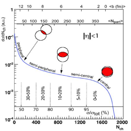
Figure 4: A cartoon showing the centrality definition from the final state particle multiplicity and its correlation with the impact parameter ($b$) and the number of participating nucleons ($N_{part}$) in the collisions.

In a collision of two nuclei, the impact parameter ($b$) can carry values from $0$ to $R_{1}+R_{2}$, where $R_{1}$ and $R_{2}$ are the diameters of the two nuclei. When $b=0$, it is called head-on collision. When collisions with $0\leq b\leq(R_{1}+R_{2})$ are allowed, it is called minimum-bias collision. In heavy-ion collisions, initial geometric quantities such as impact parameter and the collision geometry can not be directly measured experimentally. Contrary, it is however possible to relate the particle multiplicity, transverse energy and the number of spectactor nucleons (measured by a “zero-degree calorimeter” ZDC) to the centrality of the collisions.
It is straight forward to assume that on the average,
1) the energy released in a collision is proportional to the number of nucleons participating in the collisions.
2) the particle multiplicity is proportional to the participating nucleon number.
Hence the particle multiplicity is proportional to the energy released in the collision. One can measure the particle multiplicity distribution or the transverse energy ($E_{T}$) distribution for minimum-bias collisions. Here the high values of particle multiplicity or $E_{T}$ correspond to central collisions and lower values correspond to more peripheral collisions. Hence the minimum-bias $E_{T}$ or multiplicity distribution could be used for centrality determination in an collision experiment. Figure 4 shows the minimum-bias multiplicity ($N_{ch}$) distribution used for the selection of collision centrality. The minimum-bias yield has been cut into successive intervals starting from the maximum value of $N_{ch}$. The first $5\%$ of the high $N_{ch}$ events correspond to top $5\%$ central collisions. The correlation of centrality and the impact parameter with the number of participating nucleons has also been elaborated, in detail, by Glauber-type Monte Carlo calculations employing Woods-Saxon nuclear density distributions.

2.10 Number of Participants and Number of Binary Collisions

Experimentally there is no direct way to estimate the number of participating nucleons ($N_{part}$) and the number of binary collisions ($N_{bin}$) in any event, for an given impact parameter. The Glauber model calculation is performed to estimate the above two quantities as a function of the impact parameter. The Glauber model treats a nucleus-nucleus collision as a superposition of many independent nucleon-nucleon ($N-N$) collisions. This model depends on the nuclear density profile (Woods-Saxon) and the non-diffractive inelastic $N+N$ cross-sections. The Woods-Saxon distribution is given by

$$\rho(r)~{}=~{}\frac{\rho_{0}}{1+exp(\frac{r-r_{0}}{c})}$$ (78)

where, $r$ is the radial distance from the center of the nucleus, $r_{0}$ is the mean radius of the nucleus, $c$ is the skin depth of the nucleus and $\rho_{0}$ is the nuclear density constant. The parameters $r_{0}$ and $c$ are measured in electron-nucleus scattering experiments. $\rho_{0}$ is determined from the overall normalization condition

$$\int\rho(r)~{}d^{3}r~{}=~{}A$$ (79)

where $A$ is the mass number of the nucleus.

There are two separate implementations of Glauber approach: Optical and Monte Carlo (MC). In the Optical Glauber approach, $N_{part}$ and $N_{bin}$ are estimated by an analytic integration of overlapping Woods-Saxon distributions.

The MC Glauber calculation proceeds in two steps. First the nucleon position in each nucleus is determined stochastically. Then the two nuclei are “collided”, assuming the nucleons travel in a straight line along the beam axis (this is called eikonal approximation). The position of each nucleon in the nucleus is determined according to a probability density function which is typically taken to be uniform in azimuth and polar angles. The radial probability function is modeled from the nuclear charge densities extracted from electron scattering experiments. A minimum inter-nucleon separation is assumed between the positions of nucleons in a nucleus, which is the characteristic length of the repulsive nucleon-nucleon force. Two colliding nuclei are simulated by distributing $A$ nucleons of nucleus $A$ and $B$ nucleons of nucleus $B$ in 3-dimensional co-ordinate system according to their nuclear density distribution. A random impact parameter $b$ is chosen from the distribution $d\sigma/db~{}=~{}2\pi b$. A nucleus-nucleus collision is treated as a sequence of independent nucleon-nucleon collisions with a collision taking place if their distance $D$ in the transverse plane satisfies

$$D<\sqrt{\sigma_{inel}^{NN}/\pi}$$ (80)

where $\sigma_{inel}^{NN}$ is the total inelastic nucleon-nucleon cross-section. An arbitrary number of such nucleus-nucleus collisions are performed by the monte carlo and the resulting distributions of $d\sigma/N_{part}$ and $d\sigma/N_{bin}$, $d\sigma/db$ are determined. Here $N_{part}$ is defined as the total number of nucleons that underwent at least one interaction and $N_{bin}$ is the total number of interactions in an event. These histograms are binned according to fractions of the total cross-sections. This determines the mean values of $N_{part}$ and $N_{bin}$ for each centrality class. The systematic uncertainties in these values are estimated by varying the Wood-Saxon parameters, by varying the value of $\sigma_{inel}^{NN}$ and from the uncertainty in the determination of total nucleus-nucleus cross-section. These sources of uncertainties are treated as fully correlated in the final systematic uncertainty in the above measured variables.

When certain cross-sections scale with number of participants, those are said to be associated with “soft” processes: small momentum transfer processes. The low-$p_{T}$ hadron production which accounts for almost $95\%$ of the bulk hadron multiplicity comes in the “soft processes”. These soft processes are described by phenomenological non-perturbative models. Whereas, in “hard” QCD processes like jets, charmonia, other heavy flavor and processes associated with high-$p_{T}$ phenomena, the cross-section scales with the number of primordial target/projectile parton collisions. This is estimated in the above Glauber formalism as the total number of inelastic participant-participant collisions. For the hard processes the interaction is at partonic level with large momentum transfer and is governed by pQCD. $N_{coll}$ is always higher than $N_{part}$: when $N_{part}$ grows like $A$, $N_{coll}$ grows like $A^{4/3}$.

Sometimes, to study the contribution of soft and hard processes to any cross-section one takes a two-component model like:

$$cross-section~{}=~{}(1-f)~{}N_{part}~{}+~{}f~{}N_{coll}$$ (81)

where $f$ is the fractional contribution from hard processes.

3 Bulk Hadron Production in A+A Collisions

We will now take an overall look at bulk hadron production in nucleus-nucleus collisions. In view of the high total c.m. energies involved at e.g. top SPS $(E^{tot}_{cm}\approx 3.3\>TeV$) and top RHIC (38 $TeV$) energies, in central Pb+Pb (SPS) and Au+Au (RHIC) collisions, one can expect an extraordinarily high spatial density of produced particles. The average number of produced particles at SPS energies is $\approx$ 1600, while at RHIC multiplicities of $\approx$ 4000 are reached. Thus, as an overall idea of analysis, one will try to relate the observed flow of energy into transverse and longitudinal phase space and particle species to the high energy density contained in the primordial interaction volume, thus to infer about its contained matter.

Most of the particles under investigation correspond to ”thermal” pions ($p_{T}$ up to $2\>GeV$) and, in general, such thermal hadrons make up for about 95% of the observed multiplicity: the bulk of hadron production. Their distributions in phase space will be illustrated in the subsections below. This will lead to a first insight into the overall reaction dynamics, and also set the stage for consideration of the rare signals, imbedded in this thermal bulk production: direct photons, jets, heavy flavors, which are the subject of later chapters in this volume.

3.1 Particle Multiplicity and Transverse Energy Density

Particle production can be assessed globally by the total created transverse energy, the overall result of the collisional creation of transverse momentum $p_{T}$ or transverse mass ($m_{T}=\sqrt{p^{2}_{T}+m^{2}_{0}}$), at the microscopic level. Fig. 5 shows the distribution of total transverse energy $E_{T}=\sum\limits_{i}\>E(\theta_{i})\cdot sin\theta$ resulting from a calorimetric measurement of energy flow into calorimeter cells centered at angle $\theta_{i}$ relative to the beam 43 , for ${}^{32}S+^{197}$Au collisions at $\sqrt{s}=20\>GeV$, and for ${}^{208}Pb+^{208}$Pb collisions at $\sqrt{s}=17.3\>GeV$.

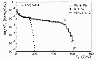
Figure 5: Minimum bias distribution of total transverse energy in Pb+Pb collisions at $\sqrt{s}=17.3\>GeV$, and S+Au collisions at $\sqrt{s}=20\>GeV$, in the rapidity interval $2.1<y<3.4$, from 43 .

The shape is characteristic of the impact parameter probability distribution (for equal size spheres in the Pb+Pb case). The turnoff at $E_{T}=520\>GeV$ indicates the point where geometry runs out of steam, i.e. where $b\rightarrow 0$, a configuration generally referred to as a ”central collision”. The adjacent shoulder results from genuine event by event fluctuations of the actual number of participant nucleons from target and projectile (recall the diffuse Woods-Saxon nuclear density profiles), and from experimental factors like calorimeter resolution and limited acceptance. The latter covers 1.3 units of pseudo-rapidity and contains mid-rapidity $\eta_{mid}=2.9$. Re-normalizing 43 to $\Delta\>\eta=1$ leads to $dE_{T}/d\eta(mid)=400\>GeV$, in agreement with the corresponding WA80 result 44 . Also, the total transverse energy of central Pb+Pb collisions at $\sqrt{s}=17.3\>GeV$ turns out to be about $1.2\>TeV$. As the definition of a central collision, indicated in Fig. 5, can be shown 42 to correspond to an average nucleon participant number of $N_{part}=370$ one finds an average total transverse energy per nucleon pair, of $E_{T}/\left<0.5\>N_{part}\right>=6.5\>GeV$. After proper consideration of the baryon pair rest mass (not contained in the calorimetric $E_{T}$ response but in the corresponding $\sqrt{s}$) one concludes 43 that the observed total $E_{T}$ corresponds to about 0.6 $E_{T}^{max}$, the maximal $E_{T}$ derived from a situation of ”complete stopping” in which the incident $\sqrt{s}$ gets fully transformed into internal excitation of a single, ideal isotropic fireball located at mid-rapidity. The remaining fraction of $E_{T}^{max}$ thus stays in longitudinal motion, reflecting the onset, at SPS energy, of a transition from a central fireball to a longitudinally extended ”fire-tube”, i.e. a cylindrical volume of high primordial energy density. In the limit of much higher $\sqrt{s}$ one may extrapolate to the idealization of a boost invariant primordial interaction volume, introduced by Bjorken 45 .

We shall show below (section 3.2) that the charged particle rapidity distributions, from top SPS to top RHIC energies, do in fact substantiate a development toward a boost-invariant situation. One may thus employ the Bjorken model for an estimate of the primordial spatial energy density $\epsilon$, related to the energy density in rapidity space via the relation 45

$$\epsilon(\tau_{0})=\frac{1}{\pi R^{2}}\>\frac{1}{\tau_{0}}\>\frac{dE_{T}}{dy}$$ (82)

where the initially produced collision volume is considered as a cylinder of length $dz=\tau_{0}dy$ and transverse radius $R\propto A^{1/3}$. Inserting for $\pi R^{2}$ the longitudinally projected overlap area of Pb nuclei colliding near head-on (”centrally”), and assuming that the evolution of primordial pQCD shower multiplication (i.e. the energy transformation into internal degrees of freedom) proceeds at a time scale $\tau_{0}\leq 1fm/c$, the above average transverse energy density, of $dE_{T}/dy=400\>GeV$ at top SPS energy 43 ; 44 leads to the estimate

$$\epsilon(\tau_{0}=1fm)=3.0\pm 0.6\>GeV/fm^{3},$$ (83)

thus exceeding, by far, the estimate of the critical energy density $\epsilon_{0}$ obtained from lattice QCD (see below), of about 1.0 $GeV/fm^{3}$. Increasing the collision energy to $\sqrt{s}=200\>GeV$ for Au+Au at RHIC, and keeping the same formation time, $\tau_{0}=1\>fm/c$ (a conservative estimate as we shall show in section 3.4), the Bjorken estimate grows to $\epsilon\approx 6.0\pm 1\>GeV/fm^{3}$. This statement is based on the increase of charged particle multiplicity density at mid-rapidity with $\sqrt{s}$, as illustrated in Fig. 6. From top SPS to top RHIC energy 46 the density per participant nucleon pair almost doubles. However, at $\sqrt{s}=200\>GeV$ the formation or thermalization time $\tau_{0}$, employed in the Bjorken model 45 , was argued 47 to be shorter by a factor of about 4. We will return to such estimates of $\tau_{0}$ in section 3.5 but note, for now, that the above choice of $\tau_{0}=1\>fm/c$ represents a conservative upper limit at RHIC energy.

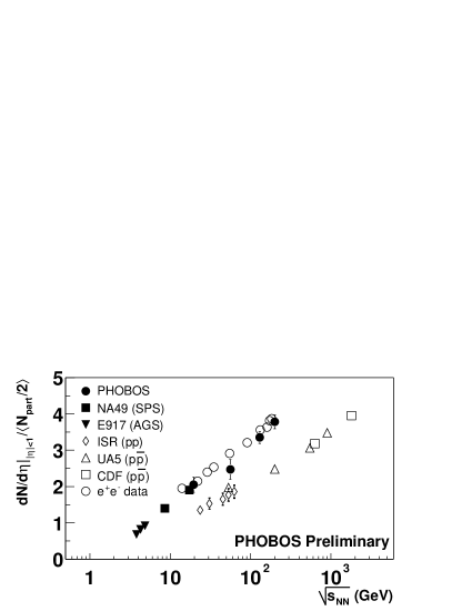
Figure 6: Charged hadron rapidity density at mid-rapidity vs. $\sqrt{s}$, compiled from $e^{+}e^{-},\>pp,\>p\overline{p}$ and A+A collisions 53 .

These Bjorken-estimates of spatial transverse energy density are confronted in Fig. 7 with lattice QCD results obtained for three dynamical light quark flavors 48 , and for zero baryo-chemical potential (as is realistic for RHIC energy and beyond but still remains a fair approximation at top SPS energy where $\mu_{B}\approx 250\>MeV)$. The energy density of an ideal, relativistic parton gas scales with the fourth power of the temperature,

$$\epsilon=gT^{4}$$ (84)

where $g$ is related to the number of degrees of freedom. For an ideal gluon gas, $g=16\>\pi^{2}/30$; in an interacting system the effective $g$ is smaller. The results of Fig. 7 show, in fact, that the Stefan-Boltzmann limit $\epsilon_{SB}$ is not reached, due to non perturbative effects, even at four times the critical temperature $T_{c}=170\>MeV$. The density $\epsilon/T^{4}=g$ is seen to ascend steeply, within the interval $T_{c}\pm 25\>MeV$. At $T_{c}$ the critical QCD energy density $\epsilon=0.6-1.0\>GeV/fm^{3}$. Relating the thermal energy density with the Bjorken estimates discussed above, one arrives at an estimate of the initial temperatures reached in nucleus-nucleus collisions, thus implying thermal partonic equilibrium to be accomplished at time scale $\tau_{0}$ (see section 3.5). For the SPS, RHIC and LHC energy domains this gives an initial temperature in the range 190 $\leq T^{SPS}\leq 220\>MeV,\>220\leq T^{RHIC}\leq 400\>MeV$ (assuming 47 that $\tau_{0}$ decreases to about 0.3 $fm/c$ here) and $T^{LHC}\geq 600\>MeV$, respectively. From such estimates one tends to conclude that the immediate vicinity of the phase transformation is sampled at SPS energy, whereas the dynamical evolution at RHIC and LHC energies dives deeply into the ”quark-gluon-plasma” domain of QCD. We shall return to a more critical discussion of such ascertations in section 3.5.

One further aspect of the mid-rapidity charged particle densities per participant pair requires attention: the comparison with data from elementary collisions. Fig. 6 shows a compilation of $pp,\>p\overline{p}$ and $e^{+}e^{-}$ data covering the range from ISR to LEP and Tevatron energies.

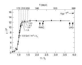
Figure 7: Lattice QCD results at zero baryon potential for energy density $\epsilon/T^{4}$ versus $T/T_{c}$ with three light quark flavors, compared to the Stefan-Boltzmann-limit $\epsilon_{SB}$ of an ideal quark-gluon gas 48 .

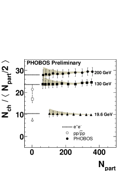
Figure 8: The total number of charged hadrons per participant pair shown as a function of $N_{part}$ in Au+Au collisions at three RHIC energies 53 .

The data from $e^{+}e^{-}$ represent $dN_{ch}/dy$, the rapidity density along the event thrust axis, calculated assuming the pion mass 49 (the difference between $dN/dy$ and $dN/d\eta$ can be ignored here). Remarkably, they superimpose with the central A+A collision data, whereas $pp$ and $p\overline{p}$ show similar slope but amount to only about 60% of the AA and $e^{+}e^{-}$ values. This difference between $e^{+}e^{-}$ annihilation to hadrons, and $pp$ or $p\overline{p}$ hadro-production has been ascribed 50 to the characteristic leading particle effect of minimum bias hadron-hadron collisions which is absent in $e^{+}e^{-}$. It thus appears to be reduced in AA collisions due to subsequent interaction of the leading parton with the oncoming thickness of the remaining target/projectile density distribution. This naturally leads to the scaling of total particle production with $N_{part}$ that is illustrated in Fig. 8, for three RHIC energies and minimum bias Au+Au collisions; the close agreement with $e^{+}e^{-}$ annihilation data is obvious again. One might conclude that, analogously, the participating nucleons get ”annihilated” at high $\sqrt{s}$, their net quantum number content being spread out over phase space (as we shall show in the next section).

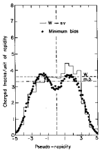
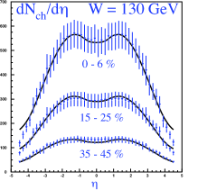
Figure 9: Left panel: charged particle pseudo-rapidity distribution in $p\overline{p}$ collisions at $\sqrt{s}=540\>GeV$ 51 . Right panel: same in RHIC Au+Au collisions at $\sqrt{s}=130\>GeV$ at different centralities 52 . Closed lines represent fits with the color glass condensate model 64 .

3.2 Rapidity Distributions

Particle production number in A+A collisions depends globally on $\sqrt{s}$ and collision centrality, and differentially on $p_{T}$ and rapidity $y$, for each particle species $i$. Integrating over $p_{T}$ results in the rapidity distribution $dN_{i}/dy$. Particle rapidity $y=sinh^{-1}\>p_{L}/M_{T}$ (where $M_{T}=\sqrt{m^{2}+p_{T}^{2}}$), requires mass identification. If that is unknown one employs pseudo-rapidity ($\eta=-\mbox{ln}\>[\mbox{tan}(\theta/2)]$) instead. This is also chosen if the joint rapidity distribution of several unresolved particle species is considered: notably the charged hadron distribution. We show two examples in Fig. 9. The left panel illustrates charged particle production in $p\overline{p}$ collisions studied by UA1 at $\sqrt{s}=540\>GeV$ 51 . Whereas the minimum bias distribution (dots) exhibits the required symmetry about the center of mass coordinate, $\eta=0$, the rapidity distribution corresponding to events in which a $W$ boson was produced (histogram) features, both, a higher average charged particle yield, and an asymmetric shape. The former effect can be seen to reflect the expectation that the $W$ production rate increases with the ”centrality” of $p\overline{p}$ collisions, involving more primordial partons as the collisional overlap of the partonic density profiles gets larger, thus also increasing the overall, softer hadro-production rate. The asymmetry should result from a detector bias favoring $W$ identification at negative rapidity: the transverse $W$ energy, of about $100\>GeV$ would locally deplete the energy store available for associated soft production. If correct, this interpretation suggests that the wide rapidity gap between target and projectile, arising at such high $\sqrt{s}$, of width $\Delta y\approx 2\>ln\>(2\gamma_{CM})$, makes it possible to define local sub-intervals of rapidity within which the species composition of produced particles varies.

The right panel of Fig. 9 shows charged particle pseudo-rapidity density distributions for Au+Au collisions at $\sqrt{s}=130\>GeV$ measured by RHIC experiment PHOBOS 52 at three different collision centralities, from ”central” (the 6% highest charged particle multiplicity events) to semi-peripheral (the corresponding 35-45% cut). We will turn to centrality selection in more detail below. Let us first remark that the slight dip at mid-rapidity and, moreover, the distribution shape in general, are common to $p\overline{p}$ and Au+Au. This is also the case for $e^{+}e^{-}$ annihilation as is shown in Fig. 10 which compares the ALEPH rapidity distribution along the mean $p_{T}$ (“thrust”) axis of jet production in $e^{+}e^{-}$ at $\sqrt{s}=200\>GeV$ 49 with the scaled PHOBOS-RHIC distribution of central Au+Au at the same $\sqrt{s}$ 53 . Note that the mid-rapidity values contained in Figs. 9 and 10 have been employed already in Fig. 6, which showed the overall $\sqrt{s}$ dependence of mid-rapidity charged particle production. What we concluded there was a perfect scaling of A+A with $e^{+}e^{-}$ data at $\sqrt{s}\geq 20\>GeV$ and a 40% suppression of the corresponding $pp,\>p\overline{p}$ yields. We see here that this observation holds, semi-quantitatively, for the entire rapidity distributions. These are not ideally boost invariant at the energies considered here but one sees in $dN_{ch}/dy$ a relatively smooth ”plateau” region extending over $\mid y\mid\leq 1.5-2.5$.

The production spectrum of charged hadrons is, by far, dominated by soft pions ($p_{T}\leq 1\>GeV/c)$ which contribute about 85% of the total yield, both in elementary and nuclear collisions. The evolution of the $\pi^{-}$ rapidity distribution with $\sqrt{s}$ is illustrated in Fig. 11 for central Au+Au and Pb+Pb collisions from AGS via SPS to RHIC energy, $2.7\leq\sqrt{s}\leq 200\>GeV$ 54 .

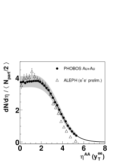
Figure 10: Pseudo-rapidity distribution of charged hadrons produced in central Au+Au collisions at $\sqrt{s}=200\>GeV$ compared with $e^{+}e^{-}$ data at similar energy. The former data normalized by $N_{part}/2$. From ref. 53 .

At lower $\sqrt{s}$ the distributions are well described by single Gaussian fits 54 with $\sigma(y)$ nearly linearly proportional to the total rapidity gap $\Delta y\propto\>ln\sqrt{s}$ as shown in the right hand panel of Fig. 11. Also illustrated is the prediction of the schematic hydrodynamical model proposed by Landau 55 ,

$$\sigma^{2}\propto ln\>(\frac{\sqrt{s}}{2m_{p}})$$ (85)

which pictures hadron production in high $\sqrt{s}$ $pp$ collisions to proceed via a dynamics of initial complete ”stopping down” of the reactants matter/energy content in a mid-rapidity fireball that would then expand via 1-dimensional ideal hydrodynamics. Remarkably, this model that has always been considered a wildly extremal proposal falls rather close to the lower $\sqrt{s}$ data for central A+A collisions but, as longitudinal phase space widens approaching boost invariance we expect that the (non-Gaussian) width of the rapidity distribution grows linearly with the rapidity gap $\Delta y$. LHC data will finally confirm this expectation, but Figs. 9 to 11 clearly show the advent of boost invariance, already at $\sqrt{s}=200\>GeV$.

A short didactic aside: At low $\sqrt{s}$ the total rapidity gap $\Delta y=2-3$ does closely resemble the total rapidity width obtained for a thermal pion velocity distribution at temperature $T=120-150\>MeV$, of a single mid-rapidity fireball, the y-distribution of which represents the longitudinal component according to the relation 19

$$\frac{dN}{dy}\propto(m^{2}T\>+\frac{2mT^{2}}{coshy}\>+\frac{2T^{2}}{cosh^{2}y})\>exp\>[-m\cdot coshy/T]$$ (86)

where $m$ is the pion mass. Any model of preferentially longitudinal expansion of the pion emitting source, away from a trivial single central ”completely stopped” fireball, can be significantly tested only once $\Delta y>3$ which occurs upward from SPS energy. The agreement of the Landau model prediction with the data in Fig. 11 is thus fortuitous, below $\sqrt{s}\approx 10\>GeV$, as any created fireball occupies the entire rapidity gap with pions.

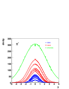
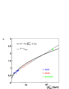
Figure 11: Left panel: negative pion rapidity distributions in central Au+Au and Pb+Pb collisions from AGS via SPS to RHIC energies 54 . Right panel: the Gaussian rapidity width of pions versus $\sqrt{s}$, confronted by Landau model predictions (solid line) 54 .

The Landau model offers an extreme view of the mechanism of ”stopping”, by which the initial longitudinal energy of the projectile partons or nucleons is inelastically transferred to produced particles and redistributed in transverse and longitudinal phase space, of which we saw the total transverse fraction in Fig. 5. Obviously $e^{+}e^{-}$ annihilation to hadrons represents the extreme stopping situation. Hadronic and nuclear collisions offer the possibility to analyze the final distribution in phase space of their non-zero net quantum numbers, notably net baryon number. Figure 12 shows the net-proton rapidity distribution (i.e. the proton rapidity distribution subtracted by the antiproton distribution) for central Pb+Pb/Au+Au collisions at AGS ($\sqrt{s}=5.5\>GeV$), SPS ($\sqrt{s}\leq 17.3\>GeV$) and RHIC ($\sqrt{s}=200\>GeV$) 56 . With increasing energy we see a central (but non-Gaussian) peak developing into a double-hump structure that widens toward RHIC leaving a plateau about mid-rapidity. The RHIC-BRAHMS experiment acceptance for $p,\>\overline{p}$ identification does unfortunately not reach up to the beam fragmentation domain at $y_{p}=5.4$ (nor does any other RHIC experiment) but only to $y\approx 3.2$, with the consequence that the major fraction of $p^{net}$ is not accounted for. However the mid-rapidity region is by no means net baryon free. At SPS energy the NA49 acceptance covers the major part of the total rapidity gap, and we observe in detail a net $p$ distribution shifted down from $y_{p}=2.9$ by an average rapidity shift 56 of $\left<\delta y\right>=1.7$. From Fig. 12 we infer that $\left<\delta y\right>$ can not scale linearly with $y_{p}\approx ln(2\gamma_{CM})\approx ln\sqrt{s}$ for ever - as it does up to top SPS energy where $\left<\delta y\right>=0.58\>y_{p}$ 56 . Because extrapolating this relation to $\sqrt{s}=200\>GeV$ would result in $\left<\delta y\right>=3.1$, and with $y_{p}\approx 5.4$ at this energy we would expect to observe a major fraction of net proton yield in the vicinity of $y=2.3$ which is not the case. A saturation must thus occur in the $\left<\delta y\right>$ vs. $\sqrt{s}$ dependence.

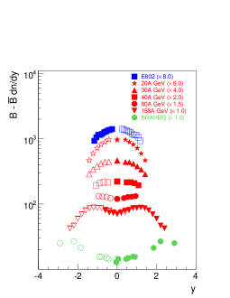
Figure 12: Net proton rapidity distributions in central Au+Au/Pb+Pb collisions at AGS, SPS and RHIC energies 56 ; 57 .

The re-distribution of net baryon density over longitudinal phase space is, of course, only partially captured by the net proton yield but a recent study 57 has shown that proper inclusion of neutron and hyperon production data at SPS and RHIC energy scales up, of course, the $dN/dy$ distributions of Fig. 12 but leaves the peculiarities of their shapes essentially unchanged. As the net baryon rapidity density distribution should resemble the final valence quark distribution the Landau model is ruled out as the valence quarks are seen to be streaming from their initial position at beam rapidity toward mid-rapidity (not vice versa). It is remarkable, however, to see that some fraction gets transported very far, during the primordial partonic non-equilibrium phase. We shall turn to its theoretical description in section 3.4 but note, for now, that $pp$ collisions studied at the CERN ISR 58 lead to a qualitatively similar net baryon rapidity distribution, albeit characterized by a smaller $\left<\delta y\right>$.

The data described above suggest that the stopping mechanism universally resides in the primordial, first generation of collisions at the microscopic level. The rapidity distributions of charged particle multiplicity, transverse energy and valence quarks exhibit qualitatively similar shapes (which also evolve similarly with $\sqrt{s}$) in $pp,\>p\overline{p},\>e^{+}e^{-}$ reactions, on the one hand, and in central or semi-peripheral collisions of $A\approx 200$ nuclei, on the other. Comparing in detail we formulate a nuclear modification factor for the bulk hadron rapidity distributions,

$$R^{AA}_{y}\>\equiv\>\frac{dN^{ch}/dy\>(y)\>\>\>\>\mathrm{in}\>\>A+A}{0.5\>N_{part}\>\>dN^{ch}/dy\>\>\>\>\mathrm{in}\>\>pp}$$ (87)

where $N_{part}<2A$ is the mean number of ”participating nucleons” (which undergo at least one inelastic collision with another nucleon) which increases with collision centrality. For identical nuclei colliding $\left<N^{proj}_{part}\right>\simeq\left<N^{targ}_{part}\right>$ and thus $0.5\>N_{part}$ gives the number of opposing nucleon pairs. $R^{AA}=1$ if each such ”opposing” pair contributes the same fraction to the total A+A yield as is produced in minimum bias $pp$ at similar $\sqrt{s}$. From Figs. 6 and 8 we infer that for $\mid\eta\mid<1,\>\>R^{AA}=1.5$ at top RHIC energy, and for the pseudo-rapidity integrated total $N^{ch}$ we find $R^{AA}=1.36$, in central Au+Au collisions. AA collisions thus provide for a higher stopping power than $pp$ (which is also reflected in the higher rapidity shift $\left<\delta y\right>$ of Fig. 12). The observation that their stopping power resembles the $e^{+}e^{-}$ inelasticity suggests a substantially reduced leading particle effect in central collisions of heavy nuclei. This might not be surprising. In a Glauber-view of successive minimum bias nucleon collisions occuring during interpenetration, each participating nucleon is struck $\nu>3$ times on average, which might saturate the possible inelasticity, removing the leading fragment.

This view naturally leads to the scaling of the total particle production in nuclear collisions with $N_{part}$, as seen clearly in Fig. 8, reminiscent of the ”wounded nucleon model” 59 but with the scaling factor determined by $e^{+}e^{-}$ rather than $pp$ 60 . Overall we conclude from the still rather close similarity between nuclear and elementary collisions that the mechanisms of longitudinal phase space population occur primordially, during interpenetration which is over after $0.15\>fm/c$ at RHIC, and after $1.5\>fm/c$ at SPS energy. I.e. it is the primordial non-equilibrium pQCD shower evolution that accounts for stopping, and its time extent should be a lower limit to the formation time $\tau_{0}$ employed in the Bjorken model 45 , equation 82. Equilibration at the partonic level might begin at $t>\tau_{0}$ only (the development toward a quark-gluon-plasma phase), but the primordial parton redistribution processes set the stage for this phase, and control the relaxation time scales involved in equilibration 61 . More about this in section 3.5. We infer the existence of a saturation scale 62 controlling the total inelasticity: with ever higher reactant thickness, proportional to $A^{1/3}$, one does not get a total rapidity or energy density proportional to $A^{4/3}$ (the number of ”successive binary collisions”) but to $A^{1.08}$ only 63 . Note that the lines shown in Fig. 9 (right panel) refer to such a saturation theory: the color glass condensate (CGC) model 64 developed by McLerran and Venugopulan. The success of these models demonstrates that ”successive binary baryon scattering” is not an appropriate picture at high $\sqrt{s}$. One can free the partons from the nucleonic parton density distributions only once, and their corresponding transverse areal density sets the stage for the ensuing QCD parton shower evolution 62 . Moreover, an additional saturation effect appears to modify this evolution at high transverse areal parton density (see section 3.4).

3.3 Dependence on system size

We have discussed above a first attempt toward a variable ($N_{part}$) that scales the system size dependence in A+A collisions. Note that one can vary the size either by centrally colliding a sequence of nuclei, $A_{1}+A_{1},\>A_{2}+A_{2}$ etc., or by selecting different windows in $N_{part}$ out of minimum bias collision ensembles obtained for heavy nuclei for which BNL employs ${}^{197}Au$ and CERN ${}^{208}Pb$. The third alternative, scattering a relatively light projectile, such as ${}^{32}S$, from increasing $A$ nuclear targets, has been employed initially both at the AGS and SPS but got disfavored in view of numerous disadvantages, of both experimental (the need to measure the entire rapidity distribution, i.e. lab momenta from about 0.3-100 $GeV$/c, with uniform efficiency) and theoretical nature (different density distributions of projectile and target; occurence of an”effectiv” center of mass, different for hard and soft collisions, and depending on impact parameter).

The determination of $N_{part}$ is of central interest, and thus we need to look at technicalities, briefly. The approximate linear scaling with $N_{part}$ that we observed in the total transverse energy and the total charged particle number (Figs. 5, 8) is a reflection of the primordial redistribution of partons and energy. Whereas all observable properties that refer to the system evolution at later times, which are of interest as potential signals from the equilibrium, QCD plasma ”matter” phase, have different specific dependences on $N_{part}$, be it suppressions (high $p_{T}$ signals, jets, quarkonia production) or enhancements (collective hydrodynamic flow, strangeness production). $N_{part}$ thus emerges as a suitable common reference scale.

$N_{part}$ captures the number of potentially directly hit nucleons. It is estimated from an eikonal straight trajectory Glauber model as applied to the overlap region arising, in dependence of impact parameter $b$, from the superposition along beam direction of the two initial Woods-Saxon density distributions of the interacting nuclei. To account for the dilute surfaces of these distributions (within which the intersecting nucleons might not find an interaction partner) each incident nucleon trajectory gets equipped with a transverse radius that represents the total inelastic NN cross section at the corresponding $\sqrt{s}$. The formalism is imbedded into a Monte Carlo simulation (for detail see 66 ) starting from random microscopic nucleon positions within the transversely projected initial Woods-Saxon density profiles. Overlapping cross sectional tubes of target and projectile nucleons are counted as a participant nucleon pair. Owing to the statistics of nucleon initial position sampling each considered impact parameter geometry thus results in a probability distribution of derived $N_{part}$. Its width $\sigma$ defines the resolution $\Delta(b)$ of impact parameter $b$ determination within this scheme via the relation

$$\frac{1}{\Delta(b)}\>\sigma(b)\approx\frac{d\left<N_{part}(b)\right>}{db}$$ (88)

which, at A=200, leads to the expectation to determine $b$ with about 1.5 $fm$ resolution 66 , by measuring $N_{part}$.

How to measure $N_{part}$? In fixed target experiments one can calorimetrically count all particles with beam momentum per nucleon and superimposed Fermi momentum distributions of nucleons, i.e. one looks for particles in the beam fragmentation domain $y_{beam}\pm 0.5,\>\>p_{T}\leq 0.25\>GeV/c$. These are identified as spectator nucleons, and $N^{proj}_{part}=A-N^{proj}_{spec}$. For identical nuclear collision systems $\left<N_{part}^{proj}\right>=\left<N_{part}^{targ}\right>$, and thus $N_{part}$ gets approximated by 2 $N_{part}^{proj}$. This scheme was employed in the CERN experiments NA49 and WA80, and generalized 67 in a way that is illustrated in Fig. 13.

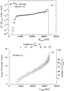
Figure 13: (a) Energy spectrum of the forward calorimeter in Pb+Pb collisions at 158$A$ GeV; (b) impact parameter and fraction of total inelastic cross section related to forward energy from the VENUS model 67 ; 68 .

The top panel shows the minimum bias distribution of total energy registered in a forward calorimeter that covers the beam fragment domain in Pb+Pb collisions at lab. energy of 158 $GeV$ per projectile nucleon, $\sqrt{s}=17.3\>GeV$. The energy spectrum extends from about $3\>TeV$ which corresponds to about 20 projectile spectators (indicating a ”central” collision), to about 32 $TeV$ which is close to the total beam energy and thus corresponds to extremely peripheral collisions. Note that the shape of this forward energy spectrum is the mirror image of the minimum bias transverse energy distribution of Fig. 5, both recorded by NA49. From both figures we see that the ideal head-on, $b\rightarrow 0$ collision can not be selected from these (or any other) data, owing to the facts that $b=0$ carries zero geometrical weight, and that the diffuse Woods-Saxon nuclear density profiles lead to a fluctuation of participant nucleon number at given finite $b$. Thus the $N_{part}$ fluctuation at finite weight impact parameters overshadows the genuinely small contribution of near zero impact parameters. Selecting ”central” collisions, either by an on-line trigger cut on minimal forward energy or maximal total transverse energy or charged particle rapidity density, or by corresponding off-line selection, one thus faces a compromise between event statistics and selectivity for impact parameters near zero. In the example of Fig. 13 these considerations suggest a cut at about $8\>TeV$ which selects the 5% most inelastic events, from among the overall minimum bias distribution, then to be labeled as ”central” collisions. This selection corresponds to a soft cutoff at $b\leq 3\>fm$.

The selectivity of this, or of other less stringent cuts on collision centrality is then established by comparison to a Glauber or cascade model. The bottom panel of Fig. 13 employs the VENUS hadron/string cascade model 68 which starts from a Monte Carlo position sampling of the nucleons imbedded in Woods-Saxon nuclear density profiles but (unlike in a Glauber scheme with straight trajectory overlap projection) following the cascade of inelastic hadron/string multiplication, again by Monte Carlo sampling. It reproduces the forward energy data reasonably well and one can thus read off the average impact parameter and participant nucleon number corresponding to any desired cut on the percent fraction of the total minimum bias cross section. Moreover, it is clear that this procedure can also be based on the total minimum bias transverse energy distribution, Fig. 5, which is the mirror image of the forward energy distribution in Fig. 13, or on the total, and even the mid-rapidity charged particle density (Fig. 8). The latter method is employed by the RHIC experiments STAR and PHENIX.

How well this machinery works is illustrated in Fig. 15 by RHIC-PHOBOS results at $\sqrt{s}=200\>GeV$ 52 . The charged particle pseudo-rapidity density distributions are shown for central (3-6% highest $N_{ch}$ cut) Cu+Cu collisions, with $\left<N_{part}\right>=100$, and semi-peripheral Au+Au collisions selecting the cut window (35-40%) such that the same $\left<N_{part}\right>$ emerges. The distributions are nearly identical. In extrapolation to $N_{part}=2$ one would expect to find agreement between min. bias $p+p$, and ”super-peripheral” A+A collisions, at least at high energy where the nuclear Fermi momentum plays no large role. Fig. 15 shows that this expectation is correct 69 . As it is technically difficult to select $N_{part}=2$ from A=200 nuclei colliding, NA49 fragmented the incident SPS Pb beam to study ${}^{12}C+^{12}C$ and ${}^{28}Si+^{28}Si$ collisions 67 . These systems are isospin symmetric, and Fig. 15 thus plots $0.5(\left<\pi^{+}\right>+\left<\pi^{-}\right>)/\left<N_{W}\right>$ including $p+p$ where $N_{W}=2$ by definition. We see that the pion multiplicity of A+A collisions interpolates to the p+p data point.

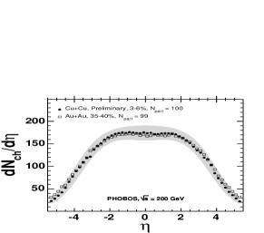
Figure 14: Charged hadron pseudo-rapidity distributions in Cu+Cu and Au+Au collisions at $\sqrt{s}=200\>GeV$, with similar $N_{part}\approx 100$ 52 .

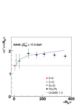
Figure 15: Charged pion multiplicity normalized by $N_{W}$ vs. centrality in p+p, C+C, Si+Si and Pb+Pb collisions at $\sqrt{s}=17.3\>GeV$ 67 ; 69 .

Note that NA49 employs the term ”wounded nucleon” number ($N_{W}$) to count the nucleons that underwent at least one inelastic nucleon-nucleon collision. This is what the RHIC experiments (that follow a Glauber model) call $N_{part}$ whereas NA49 reserves this term for nucleons that underwent any inelastic collision. Thus $N_{W}$ in Fig. 15 has the same definition as $N_{part}$ in Figs. 6, 8, 10, 15. We see that a smooth increase joins the $p+p$ data, via the light A+A central collisions, to a saturation setting in with semi-peripheral Pb+Pb collisions, the overall, relative increase amounting to about 40% (as we saw in Fig. 6).

There is nothing like an $N_{part}^{1/3}$ increase (the thickness of the reactants) observed here, pointing to the saturation mechanism(s) mentioned in the previous section, which are seen from Fig. 15 to dampen the initial, fast increase once the primordial interaction volume contains about 80 nucleons. In the Glauber model view of successive collisions (to which we attach only symbolical significance at high $\sqrt{s}$) this volume corresponds to $\left<\nu\right>\approx 3$, and within the terminology of such models we might thus argue, intuitively, that the initial geometrical cross section, attached to the nucleon structure function as a whole, has disappeared at $\left<\nu\right>\approx 3$, all constituent partons being freed.

3.4 Gluon Saturation in A+A Collisions

We will now take a closer look at the saturation phenomena of high energy QCD scattering, and apply results obtained for deep inelastic electron-proton reactions to nuclear collisions, a procedure that relies on a universality of high energy scattering. This arises at high $\sqrt{s}$, and at relatively low momentum transfer squared $Q^{2}$ (the condition governing bulk charged particle production near mid-rapidity at RHIC, where Feynman $x\approx 0.01$ and $Q^{2}\leq 5\>GeV^{2}$). Universality comes about as the transverse resolution becomes higher and higher, with $Q^{2}$, so that within the small area tested by the collision there is no difference whether the partons sampled there belong to the transverse gluon and quark density projection of any hadron species, or even of a nucleus. And saturation arises once the areal transverse parton density exceeds the resolution, leading to interfering QCD sub-amplitudes that do not reflect in the total cross section in a manner similar to the mere summation of separate, resolved color charges 61 ; 62 ; 63 ; 64 ; 65 ; 70 ; 71 .

The ideas of saturation and universality are motivated by HERA deep inelastic scattering (DIS) data 72 on the gluon distribution function shown in Fig. 16 (left side). The gluon rapidity density, $xG(x,Q^{2})=\frac{dN^{gluon}}{dy}$ rises rapidly as a function of decreasing fractional momentum, $x$, or increasing resolution, $Q^{2}$. The origin of this rise in the gluon density is, ultimately, the non-abelian nature of QCD. Due to the intrinsic non-linearity of QCD 70 ; 71 , gluon showers generate more gluon showers, producing an avalanche toward small $x$. As a consequence of this exponential growth the spatial density of gluons (per unit transverse area per unit rapidity) of any hadron or nucleus must increase as $x$ decreases 65 . This follows because the transverse size, as seen via the total cross section, rises more slowly toward higher energy than the number of gluons. This is illustrated in Fig. 16 (right side). In a head-on view of a hadronic projectile more and more partons (mostly gluons) appear as $x$ decreases. This picture reflects a representation of the hadron in the ”infinite momentum frame” where it has a large light-cone longitudinal momentum $P^{+}\gg M$. In this frame one can describe the hadron wave function as a collection of constituents carrying a fraction $p^{+}=xP^{+},\>0\leq x<1$, of the total longitudinal momentum 73 (”light cone quantization” method 74 ). In DIS at large $\sqrt{s}$ and $Q^{2}$ one measures the quark distributions $dN_{q}/dx$ at small $x$, deriving from this the gluon distributions $xG(x,Q^{2})$ of Fig. 16.

It is useful 75 to consider the rapidity distribution implied by the parton distributions, in this picture. Defining $y=y_{hadron}-ln(1/x)$ as the rapidity of the potentially struck parton, the invariant rapidity distribution results as

$$dN/dy=x\>dN/dx=xG(x,Q^{2}).$$ (89)

At high $Q^{2}$ the measured quark and gluon structure functions are thus simply related to the number of partons per unit rapidity, resolved in the hadronic wave function.

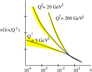
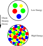
Figure 16: (left) The HERA data for the gluon distribution function as a function of fractional momentum $x$ and square momentum transfer $Q^{2}$ 72 . (right) Saturation of gluons in a hadron; a head on view as $x$ decreases 75 .

The above textbook level 74 ; 75 recapitulation leads, however, to an important application: the $dN/dy$ distribution of constituent partons of a hadron (or nucleus), determined by the DIS experiments, is similar to the rapidity distribution of produced particles in hadron-hadron or A+A collisions as we expect the initial gluon rapidity density to be represented in the finally observed, produced hadrons, at high $\sqrt{s}$. Due to the longitudinal boost invariance of the rapidity distribution, we can apply the above conclusions to hadron-hadron or A+A collisions at high $\sqrt{s}$, by replacing the infinite momentum frame hadron rapidity by the center of mass frame projectile rapidity, $y_{proj}$, while retaining the result that the rapidity density of potentially interacting partons grows with increasing distance from $y_{proj}$ like

$$\Delta y\equiv y_{proj}-y=ln(1/x).$$ (90)

At RHIC energy, $\sqrt{s}=200\>GeV$, $\Delta y$ at mid-rapidity thus corresponds to $x<10^{-2}$ (well into the domain of growing structure function gluon density, Fig. 16), and the two intersecting partonic transverse density distributions thus attempt to resolve each other given the densely packed situation that is depicted in the lower circle of Fig. 16 (right panel). At given $Q^{2}$ (which is modest, $Q^{2}\leq 5\>GeV^{2}$, for bulk hadron production at mid-rapidity) the packing density at mid-rapidity will increase toward higher $\sqrt{s}$ as

$$\Delta y^{midrap}\approx ln(\sqrt{s}/M),\>i.e.\>1/x\approx\sqrt{s}/M$$ (91)

thus sampling smaller $x$ domains in Fig. 16 according to equation 90. It will further increase in proceeding from hadronic to nuclear reaction partners A+A. Will it be in proportion to $A^{4/3}$? We know from the previous sections (3.2 and 3.3) that this is not the case, the data indicating an increase with $A^{1.08}$. This observation is, in fact caused by the parton saturation effect, to which we turn now.

For given transverse resolution $Q^{2}$ and increasing $1/x$ the parton density of Fig. 16 becomes so large that one can not neglect their mutual interactions any longer. One expects such interactions to produce ”shadowing”, a decrease of the scattering cross section relative to incoherent independent scattering 70 ; 71 . As an effect of such shadowed interactions there occurs 75 a saturation 61 ; 62 ; 63 ; 64 ; 65 ; 70 ; 71 ; 75 of the cross section at each given $Q^{2}$, slowing the increase with $1/x$ to become logarithmic once $1/x$ exceeds a certain critical value $x_{s}(Q^{2})$. Conversely, for fixed $x$, saturation occurs for transverse momenta below some critical $Q^{2}(x)$,

$$Q_{s}^{2}(x)=\alpha_{s}N_{c}\>\frac{1}{\pi R^{2}}\>\frac{dN}{dy}$$ (92)

where $dN/dy$ is the $x$-dependent gluon density (at $y=y_{proj}-ln(1/x))$. $Q^{2}_{s}$ is called the saturation scale. In equation 92 $\pi R^{2}$ is the hadron area (in transverse projection), and $\alpha_{s}N_{c}$ is the color charge squared of a single gluon. More intuitively, $Q^{2}_{s}(x)$ defines an inversely proportional resolution area $F_{s}(x)$ and at each $x$ we have to choose $F_{s}(x)$ such that the ratio of total area $\pi R^{2}$ to $F_{s}(x)$ (the number of resolved areal pixels) equals the number of single gluon charge sources featured by the total hadron area. As a consequence the saturation scale $Q^{2}_{s}(x)$ defines a critical areal resolution, with two different types of QCD scattering theory defined, at each $x$, for $Q^{2}>Q^{2}_{s}$ and $Q^{2}<Q^{2}_{s}$, respectively 62 ; 65 ; 75 .

As one expects a soft transition between such theories, to occur along the transition line implied by $Q^{2}_{s}(x)$, the two types of QCD scattering are best studied with processes featuring typical $Q^{2}$ well above, or below $Q^{2}_{s}(x)$. Jet production at $\sqrt{s}\geq 200\>GeV$ in $p\overline{p}$ or AA collisions with typical $Q^{2}$ above about $10^{3}\>GeV^{2}$, clearly falls into the former class, to be described e.g. by perturbative QCD DGLAP evolution of partonic showers 76 . The accronym DGLAP refers to the inventors of the perturbative QCD evolution of parton scattering with the ”runing” strong coupling constant $\alpha_{s}(Q^{2})$, Dokshitzer, Gribov, Levine, Altarelli and Parisi. On the other hand, mid-rapidity bulk hadron production at the upcoming CERN LHC facility ($\sqrt{s}=14\>TeV$ for $pp$, and $5.5\>TeV$ for A+A), with typical $Q^{2}\leq 5\>GeV^{2}$ at $x\leq 10^{-3}$, will present a clear case for QCD saturation physics, as formulated e.g. in the ”Color Glass Condensate (CGC)” formalism developed by McLerran, Venugopalan and collaborators 64 ; 65 ; 75 ; 77 . This model develops a classical gluon field theory for the limiting case of a high areal occupation number density, i.e for the conceivable limit of the situation depicted in Fig. 16 (right hand panel) where the amalgamating small $x$ gluons would overlap completely, within any finite resolution area at modest $Q^{2}$. Classical field theory captures, by construction, the effects of color charge coherence, absent in DGLAP parton cascade evolution theories 75 . This model appears to work well already at $\sqrt{s}$ as ”low” as at RHIC, as far as small $Q^{2}$ bulk charged particle production is concerned. We have illustrated this by the CGC model fits 64 to the PHOBOS charged particle rapidity distributions, shown in Fig. 9.

Conversely, QCD processes falling in the transition region between such limiting conditions, such that typical $Q^{2}\approx Q^{2}_{s}(x)$, should present observables that are functions of the ratio between the transferred momentum $Q^{2}$ and the appropriate saturation scale, expressed by $Q^{2}_{s}(x)$. As $Q^{2}$ defines the effective transverse sampling area, and $Q^{2}_{s}(x)$ the characteristic areal size at which saturation is expected to set in, a characteristic behaviour of cross sections, namely that they are universal functions of $Q^{2}/Q^{2}_{s}$, is called ”geometric scaling”. The HERA ep scattering data obey this scaling law closely 78 , and the idea arises to apply the universality principle that we mentioned above: at small enough $x$, all hadrons or nuclei are similar, their specific properties only coming in via the appropriate saturation scales $Q^{2}_{s}(x,h)$ or $Q^{2}_{s}(x,A)$. Knowing the latter for RHIC conditions we will understand the systematics of charged particle production illustrated in the previous section, and thus also be able to extrapolate toward LHC conditions in $pp$ and AA collisions.

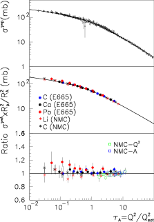
Figure 17: (top) Geometric scaling of the virtual photo-absorption cross section $\sigma^{\gamma p}$ on protons; (middle) cross sections for nuclei normalized according to equation 94; (bottom) the ratio of $\sigma^{\gamma A}$ to a fit of $\sigma^{\gamma p}$ (see 63 for data reference).

All data for the virtual photo-absorption cross section $\sigma^{\gamma p}(x,Q^{2})$ in deep inelastic ep scattering with $x\leq 0.01$ (which is also the RHIC mid-rapidity $x$-domain) have been found 78 to lie on a single curve when plotted against $Q^{2}/Q^{2}_{s}$, with

$$Q_{s}^{2}(x)\sim(\frac{x_{0}}{x})^{\lambda}\>1GeV^{2}$$ (93)

with $\lambda\simeq 0.3$ and $x_{0}\simeq 10^{-4}$. This scaling 79 with $\tau=Q^{2}/Q^{2}_{s}$ is shown in Fig. 17 (top panel) to interpolate all data. A chain of arguments, proposed by Armesto, Salgado and Wiedemann 63 connects a fit to these data with photo-absorption data for (virtual) photon-A interactions 80 via the geometrical scaling ansatz

$$\frac{\sigma^{\gamma A}(\tau_{A})}{\pi R^{2}_{A}}=\frac{\sigma^{\gamma p}(\tau_{p}=\tau_{A})}{\pi R^{2}_{p}}$$ (94)

assuming that the scale in the nucleus grows with the ratio of the transverse parton densities, raised to the power $1/\delta$ (a free parameter),

$$Q^{2}_{s,A}=Q^{2}_{s,p}\left(\frac{A\pi R^{2}_{p}}{\pi R^{2}_{A}}\right)^{1/\delta},\>\>\tau_{A}=\tau_{h}\left(\frac{\pi R^{2}_{A}}{A\pi R^{2}_{h}}\right)^{1/\delta}.$$ (95)

Fig. 17 (middle and bottom panels) shows their fit to the nuclear photo-absorbtion data which fixes $\delta=0.79$ and $\pi R^{2}_{p}=1.57\>fm^{2}$ (see ref. 63 for detail). The essential step in transforming these findings to the case of A+A collisions is then taken by the empirical ansatz

$$\frac{dN^{AA}}{dy}\>(at\>y\simeq 0)\>\propto\>Q^{2}_{s,A}(x)\pi R^{2}_{A}$$ (96)

by which the mid-rapidity parton (gluon) density $dN/dy$ in equation 92 gets related to the charged particle mid-rapidity density at $y\approx 0$ 70 ; 81 , measured in nucleus-nucleus collisions. Replacing, further, the total nucleon number 2A in a collision of identical nuclei of mass A by the number $N_{part}$ of participating nucleons, the final result is 63

$$\frac{1}{N_{part}}\>\>\frac{dN^{AA}}{dy}\>(at\>y\approx 0)=N_{0}(\sqrt{s})^{\lambda}\>N^{\alpha}_{part}$$ (97)

where the exponent $\alpha\equiv(1-\delta)/3\delta=0.089$, and $N_{0}=0.47$. The exponent $\alpha$ is far smaller than 1/3, a value that represents the thickness of the reactants, and would be our naive guess in a picture of ”successive” independent nucleon participant collisions, whose average number $\left<\nu\right>\>\propto\>(N_{part}/2)^{1/3}$. The observational fact (see Fig. 15) that $\alpha<1/3$ for mid-rapidity low $Q^{2}$ bulk hadron production in A+A collisions illustrates the importance of the QCD saturation effect. This is shown 63 in Fig. 18 where equation 97 is applied to the RHIC PHOBOS data for mid-rapidity charged particle rapidity density per participant pair, in Au+Au collisions at $\sqrt{s}=19.6$, 130 and 200 $GeV$ 82 , also including a prediction for LHC energy. Note that the factorization of energy and centrality dependence, implied by the RHIC data 52 , is well captured by equation 92 and the resulting fits in Fig. 18. Furthermore, the steeper slope, predicted for $N_{part}\leq 60$ (not covered by the employed data set), interpolates to the corresponding $pp$ and $p\overline{p}$ data, at $N_{part}=2$. It resembles the pattern observed in the NA49 data (Fig. 15) for small $N_{part}$ collisions of light A+A systems, at $\sqrt{s}=17-20\>GeV$, and may be seen, to reflect the onset of QCD saturation. Finally we note that the conclusions of the above, partially heuristic approach 63 , represented by equations 94 to 97, have been backed up by the CGC theory of McLerran and Venugopulan 64 ; 65 ; 75 , predictions of which we have illustrated in Fig. 9.

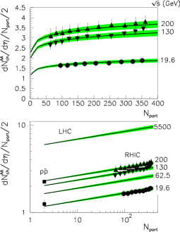
Figure 18: Saturation model fit 63 applied to RHIC charged hadron multiplicity data at mid-rapidity normalized by number of participant pairs, at various energies 82 . Also shown is an extrapolation to $p\overline{p}$ data and a prediction for minimum bias Pb+Pb collisions at LHC energy, $\sqrt{s}=5500\>GeV$.

Bulk hadron production in AA collisions at high $\sqrt{s}$ can be related, via the assumption of universality of high energy QCD scattering, to the phenomenon of geometric scaling first observed in HERA deep inelastic ep cross sections. The underlying feature is a QCD saturation effect arising from the diverging areal parton density, as confronted with the limited areal resolution $Q^{2}$, inherent in the considered scattering process. The ”saturation scale” $Q^{2}_{s}(x,A)$ captures the condition that a single partonic charge source within the transverse partonic density profile can just be resolved by a sufficiently high $Q^{2}$. Bulk hadron production in A+A collisions falls below this scale.

3.5 Transverse phase space: equilibrium and the QGP state

At RHIC energy, $\sqrt{s}=200\>GeV$, the Au+Au collision reactants are longitudinally contracted discs. At a nuclear radius $R\approx A^{1/3}\>fm$ and Lorentz $\gamma\approx 100$ their primordial interpenetration phase ends at time $\tau_{0}\leq 0.15\>fm/c$. This time scale is absent in $e^{+}e^{-}$ annihilation at similar $\sqrt{s}$ where $\tau_{0}\approx 0.1\>fm/c$ marks the end of the primordial pQCD partonic shower evolution 83 during which the initially created $q\overline{q}$ pair, of ”virtually” $Q=\sqrt{s}/2$ each, multiplies in the course of the QCD DGLAP evolution in perturbative vacuum, giving rise to daughter partons of far lower virtuality, of a few $GeV$. In A+A collisions this shower era should last longer, due to the interpenetrational spread of primordial collision time. It should be over by about 0.25 $fm/c$. The shower partons in $e^{+}e^{-}$ annihilation stay localized within back to back cone geometry reflecting the directions of the primordial quark pair. The eventually observed ”jet” signal, created by an initial $Q^{2}$ of order $10^{4}\>GeV^{2}$, is established by then. Upon a slow-down of the dynamical evolution time scale to $\tau\approx 1\>fm/c$ the shower partons fragment further, acquiring transverse momentum and yet lower virtuality, then to enter a non perturbative QCD phase of color neutralization during which hadron-like singlet parton clusters are formed. Their net initial pQCD virtuality, in pQCD vacuum, is recast in terms of non-perturbative vacuum hadron mass. The evolution ends with on-shell, observed jet-hadrons after about $3\>fm/c$ of overall reaction time.

Remarkably, even in this, somehow most elementary process of QCD evolution, an aspect of equilibrium formation is observed, not in the narrowly focussed final dijet momentum topology but in the relative production rates of the various created hadronic species. This so-called ”hadrochemical” equilibrium among the hadronic species is documented in Fig. 19. The hadron multiplicities per $e^{+}e^{-}$ annihilation event at $\sqrt{s}=91.2\>GeV$ 38 are confronted with a Hagedorn 38 canonical statistical Gibbs ensemble prediction 84 which reveals that the apparent species equilibrium was fixed at a temperature of $T=165\>MeV$, which turns out to be the universal hadronization temperature of all elementary and nuclear collisions at high $\sqrt{s}$ (Hagedorns limiting temperature of the hadronic phase of matter). We shall return to this topic in section 4 but note, for now, that reactions with as few as 20 charged particles exhibit such statistical equilibrium properties.

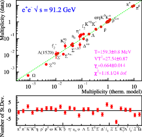
Figure 19: Hadron multiplicities in LEP $e^{+}e^{-}$ annihilation at $\sqrt{s}=91.2\>GeV$ confronted with the predictions of the canonical statistical hadronization model 84 .

What happens with parton (and hadron) dynamics in A+A collisions after $\tau_{0}$? There will not be a QCD evolution in vacuum as the transverse radius of the interacting system is large. It may grow to about twice the nuclear radius, i.e. to about $15\>fm$ before interactions cease; i.e. the system needs about $15\>fm/c$ to decouple. This simple fact is the key to our expectation that the expansive evolution of the initial high energy density deposited in a cylinder of considerable diameter (about $10\>fm$), may create certain equilibrium properties that allow us to treat the contained particles and energy in terms of thermodynamic phases of matter, such as a partonic QGP liquid, or a hadronic liquid or gas, etc.. Such that the expansion dynamics makes contact to the phase diagram illustrated in Fig. 1. This expectation turns out to be justified as we shall describe in section 4. What results for the evolution after $\tau_{0}$ in a central A+A collision is sketched in Fig. 2 by means of a schematic 2-dimensional light cone diagram, which is entered by the two reactant nuclei along $\pm z=t$ trajectories where $z$ is the beam direction and Lorentz contraction has been taken to an extreme, such that there occurs an idealized $t=z=0$ interaction ”point”. Toward positive $t$ the light cone proper time profiles of progressing parton-hadron matter evolution are illustrated. The first profile illustrated here corresponds to the end of shower formation time $\tau_{0}$. From our above discussion of the $e^{+}e^{-}$ annihilation process one obtains a first estimate, $\tau_{0}\geq 0.25\>fm/c$ (including interpenetration time of 0.15 $fm/c$ at RHIC) which refers to processes of very high $Q^{2}\geq 10^{3}\>GeV^{2}$, far above the saturation scale $Q^{2}_{s}$ discussed in the previous section. The latter scale has to be taken into account for low $p_{T}$ hadron production.

It is the specific resolution scale $Q^{2}$ of a QCD sub-process, as enveloped in the overall collision dynamics of two slabs of given transverse partonic structure function density, that determines which fraction of the constituent partons enters interaction. In the simple case of extremely high $Q^{2}$ processes the answer is that all constituents are resolved. However, at modest $Q^{2}$ (dominating bulk hadron production) the characteristic QCD saturation scale $Q^{2}_{s}(x)$ gains prominence, defined such that processes with $Q^{2}<Q^{2}_{s}$ do not exploit the initial transverse parton densities at the level of independent single constituent color field sources (see equation 92). For such processes the proper formation time scale, $\tau_{0}$, is of order of the inverse saturation momentum 61 , $1/Q_{s}\sim 0.2\>fm/c$ at $\sqrt{s}=200\>GeV$. The first profile of the time evolution, sketched in Fig. 2, should correspond to proper time $t=\tau_{0}=0.25\>fm/c$ at RHIC energy. At top SPS energy, $\sqrt{s}=17.3\>GeV$, we can not refer to such detailed QCD considerations. A pragmatic approach suggests to take the interpenetration time, at $\gamma\approx 8.5$, for guidance concerning the formation time, which thus results as $\tau_{0}\approx 1.5\>fm/c$.

In summary of the above considerations we assume that the initial partonic color sources, as contained in the structure functions (Fig. 16), are spread out in longitudinal phase space after light cone proper time $t=\tau_{0}\approx 0.25\>fm/c$, at top RHIC energy, and after $\tau_{0}\approx 1.4\>fm/c$ at top SPS energy. No significant transverse expansion has occured at this early stage, in a central collision of $A\approx 200$ nuclei with transverse diameter of about 12 $fm$. The Bjorken estimate 45 of initial energy density $\epsilon$ (equation 82) refers to exactly this condition, after formation time $\tau_{0}$. In order to account for the finite longitudinal source size and interpenetration time, at RHIC, we finally put the average $\tau_{0}\approx 0.3\>fm$, at $\sqrt{s}=200\>GeV$, indicating the ”initialization time” after which all partons that have been resolved from the structure functions are engaged in shower multiplication. As is apparent from Fig. 2, this time scale is Lorentz dilated for partons with a large longitudinal momentum, or rapidity. This means that the slow particles are produced first toward the center of the collision region, and the fast (large rapidity) particles are produced later, away from the collision region. This Bjorken ”inside-out” correlation 45 between coordinate- and momentum-space is similar to the Hubble expansion pattern in cosmology: more distant galaxies have higher outward velocities. Analogously, the matter created in A+A collisions at high $\sqrt{s}$ is born expanding, however with the difference that the Hubble flow is initially one dimensional along the collision axis. This pattern will continue, at $\sqrt{s}=200\>GeV$, until the system begins to feel the effects of finite size in the transverse direction which will occur at some time $t_{0}$ in the vicinity of $1\>fm/c$. However, the tight correlation between position and momentum initially imprinted on the system will survive all further expansive evolution of the initial ”firetube”, and is well recovered in the expansion pattern of the finally released hadrons of modest $p_{T}$ as we shall show when discussing radial flow (see section 3.6).

In order to proceed to a more quantitative description of the primordial dynamics (that occurs onward from $\tau_{0}$ for as long the time period of predominantly longitudinal expansion might extend) we return to the Bjorken estimate of energy density, corresponding to this picture 45 , as implied by equation 82, which we now recast as

$$\epsilon=\left(\frac{dN_{h}}{dy}\right)\left<E^{T}_{h}\right>(\pi\>R^{2}_{A}\>t_{0})^{-1}$$ (98)

where the first term is the (average) total hadron multiplicity per unit rapidity which , multiplied with the average hadron transverse energy, equals the total transverse energy recorded in the calorimetric study shown in Fig. 5, as employed in equation 82. The quantity $R_{A}$ is, strictly speaking, not the radius parameter of the spherical Woods-Saxon nuclear density profile but the $rms$ of the reactant overlap profiles as projected onto the transverse plane (and thus slightly smaller than $R_{A}\approx A^{1/3}\>fm$). Employing $A^{1/3}$ here (as is done throughout) leads to a conservative estimate of $\epsilon$, a minor concern. However, the basic assumption in equation 98 is to identify the primordial transverse energy ”radiation”, of an interactional cylindric source of radius $R_{A}$ and length $t_{0}$ (where $\tau_{0}\leq t_{0}\leq 1\>fm/c$, not Lorentz dilated at midrapidity), with the finally emerging bulk hadronic transverse energy. We justify this assumption by the two observations, made above, that

1. the bulk hadron multiplicity density per unit rapidity $\frac{dN_{h}}{dy}$ resembles the parton density, primordially released at saturation scale $\tau_{0}$ (Figs. 9, 18) at $\sqrt{s}=200\>GeV$, and that

2. the global emission pattern of bulk hadrons (in rapidity and $p_{T}$) closely reflects the initial correlation between coordinate and momentum space, characteristic of a primordial period of a predominantly longitudinal expansion, as implied in the Bjorken model.

Both these observations are surprising, at first sight. The Bjorken model was conceived for elementary hadron collisions where the expansion proceeds into vacuum, i.e. directly toward observation. Fig. 2 proposes that, to the contrary, primordially produced partons have to transform through further, successive stages of partonic and hadronic matter, at decreasing but still substantial energy density, in central A+A collisions. The very fact of high energy density, with implied short mean free path of the constituent particles, invites a hydrodynamic description of the expansive evolution. With initial conditions fixed between $\tau_{0}$ and $t_{0}$, an ensuing 3-dimensional hydrodynamic expansion would preserve the primordial Bjorken-type correlation between position and momentum space, up to lower density conditions and, thus, close to emission of the eventually observed hadrons. We thus feel justified to employ equation 82 or 98 for the initial conditions at RHIC, obtaining 61 ; 84

$$6\>GeV/fm^{3}\leq\epsilon\leq 20\>GeV/fm^{3}$$ (99)

for the interval $0.3\>fm/c\leq t_{0}\leq 1\>fm/c$, in central Au+Au collisions at $y\approx 0$ and $\sqrt{s}=200\>GeV$. The energy density at top SPS energy, $\sqrt{s}=17.3\>GeV$, can similarly be estimated 43 ; 44 to amount to about $3\>GeV/fm^{3}$ at a $t_{0}$ of 1 $fm/c$ but we can not identify conditions at $\tau_{0}<t_{0}$ in this case as the mere interpenetration of two Pb nuclei takes $1.4\>fm/c$. Thus the commonly accepted $t_{0}=1\>fm/c$ may lead to a high estimate. An application of the parton-hadron transport model of Ellis and Geiger 85 ; 86 to this collision finds $\epsilon=3.3\>GeV/fm^{3}$ at $t=1\>fm/c$. A primordial energy density of about $3\>GeV/fm^{3}$ is twenty times $\rho_{0}\approx 0.15\>GeV/fm^{3}$, the average energy density of ground state nuclear matter, and it also exceeds, by far, the critical QCD energy density, of $0.6\leq\epsilon_{c}\leq 1\>GeV/fm^{3}$ according to lattice QCD 48 . The initial dynamics thus clearly proceeds in a deconfined QCD system also at top SPS energy, and similarly so with strikingly higher energy density, at RHIC, where time scales below $1\>fm/c$ can be resolved.

However, in order now to clarify the key question as to whether, and when conditions of partonic dynamical equilibrium may arise under such initial conditions, we need estimates both of the proper relaxation time scale (which will, obviously, depend on energy density and related collision frequency), and of the expansion time scale as governed by the overall evolution of the collision volume. Only if $\tau(relax.)<\tau(expans.)$ one may conclude that the ”deconfined partonic system” can be identified with a ”deconfined QGP state of QCD matter” as described e.g. by lattice QCD, and implied in the phase diagram of QCD matter suggested in Fig. 1.

For guidance concerning the overall time-order of the system evolution we consider information 87 obtained from Bose-Einstein correlation analysis of pion pair emission in momentum space. Note that pions should be emitted at any stage of the evolution, after formation time, from the surface regions of the evolving ”fire-tube”. Bulk emission of pions occurs, of course, after hadronization (the latest stages illustrated in the evolution sketch given in Fig. 2). The dynamical pion source expansion models by Heinz 88 and Sinyukov 89 elaborate a Gaussian emission time profile, with mean $\tau_{f}$ (the decoupling time) and width $\Delta\tau$ (the duration of emission).

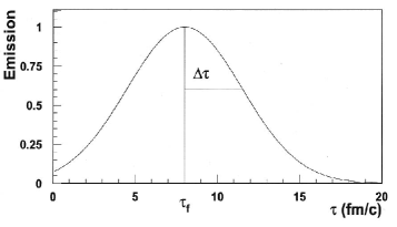
Figure 20: Time profile of pion decoupling rate from the fireball in a central Pb+Pb collision, with $\tau=0$ the end of the formation phase. Bose-Einstein correlation of $\pi^{-}\pi^{-}$pairs yields an average Gaussian decoupling profile with $\tau_{f}=8\>fm/c$ and duration of emission parameter $\Delta\tau=4\>fm/c$ 87 ; 88 .

Fig. 20 shows an application of this analysis to central Pb+Pb collision negative pion pair correlation data obtained by NA49 at top SPS energy, $\sqrt{s}=17.3\>GeV$ 90 , where $\tau_{f}\approx 8\>fm/c$ and $\Delta\tau\approx 4\>fm/c$ (note that $\tau=0$ in Fig. 20 corresponds, not to interaction time $t=0$ but to $t\approx 1.4\>fm/c$, the end of the interpenetration phase). We see, first of all, that the overall dynamical evolution of a central Pb+Pb collision at $\sqrt{s}=17.3\>GeV$ is ending at about $15\>fm/c$; the proper time defines the position of the last, decoupling profile illustrated in Fig. 2, for the SPS collisions considered here. While the details of Fig. 20 will turn out to be relevant to our later discussion of hadronization (section 4) and hadronic expansion, we are concerned here with the average proper time at which the partonic phase ends. After consideration of the duration widths of these latter expansion phases 86 ; 87 one arrives at an estimate for the average time, spent before hadronization, of $\Delta t=3-4\>fm/c$, again in agreement with the parton cascade model mentioned above 86 . This model also leads to the conclusion that parton thermal equilibrium is, at least, closely approached locally in these central Pb+Pb collisions as far as mid-rapidity hadron production is concerned (at forward-backward rapidity the cascade re-scattering processes do not suffice, however).

This finding agrees with earlier predictions of $\tau_{relax}=1-2\>fm/c$ at top SPS energy 91 . However we note that all such calculations employ perturbative QCD methods, implying the paradoxical consequence that equilibrium is closely approached toward the end of the partonic phase, at such low $\sqrt{s}$, i.e. in a QGP state at about $T=200\>MeV$ which is, by definition, of non-perturbative nature. We shall return to the question of partonic equilibrium attainment at SPS energy in the discussion of the hadronization process in nuclear collisions (section 4).

Equilibrium conditions should set in earlier at top RHIC energy. As transverse partonic expansion should set in after the proper time interval $0.3\>fm/c\leq t_{0}\leq 1\>fm/c$ (which is now resolved by the early dynamics, unlike at top SPS energy), we take guidance from the Bjorken estimate of primordial energy density which is based on transverse energy production data. Conservatively interpreting the result in equation 99 we conclude that $\epsilon$ is about four times higher than at $\sqrt{s}=17.3\>GeV$ in the above proper time interval. As the binary partonic collision frequency scales with the square of with the square of the density $\rho$ (related to the energy density $\epsilon$ via the relation $\epsilon$ = $\left<E\right>\rho$ = $T\rho$), and is inversely proportional to the relaxation time $\tau_{relax}$ we expect

$$\tau_{relax}\propto(1/\rho)^{2}\approx(T/\epsilon)^{2}$$ (100)

which implies that $\tau_{relax}(RHIC)\approx 0.25\>\tau_{relax}(SPS)\approx 0.5\>fm/c$ if we employ the estimate $T(RHIC)\>=\>2T(SPS)$. This crude estimate is, however, confirmed by the parton transport model of Molar and Gyulassy 92 .

Partonic equilibration at $\sqrt{s}=200\>GeV$ should thus set in at a time scale commensurate to the (slightly smaller) formation time scale, at which the to be participant partons are resolved from the initial nucleon structure functions and enter shower multiplication. Extrapolating to the conditions expected at LHC energy ($\sqrt{s}=5.5\>TeV$ for A+A collisions), where the initial parton density of the structure functions in Fig. 16 is even higher ($x\approx 10^{-3}$ at mid-rapidity), and so is the initial energy density, we may expect conditions at which the resolved partons are almost ”born into equilibrium”.

Early dynamical local equilibrium at RHIC is required to understand the observations concerning elliptic flow. This term refers to a collective anisotropic azimuthal emission pattern of bulk hadrons in semi-peripheral collisions, a hydrodynamical phenomenon that originates from the initial geometrical non-isotropy of the primordial interaction zone 93 ; 94 . A detailed hydrodynamic model analysis of the corresponding elliptic flow signal at RHIC 95 leads to the conclusion that local equilibrium (a prerequisite to the hydrodynamic description) sets in at $t_{0}\approx 0.5\>fm/c$. This conclusion agrees with the estimate via equation 100 above, based on Bjorken energy density and corresponding parton collisions frequency.

We note that the concept of a hydrodynamic evolution appears to be, almost necessarily ingrained in the physics of a system born into (Hubble-type) expansion, with a primordial correlation between coordinate and momentum space, and at extreme initial parton density at which the partonic mean free path length $\lambda$ is close to the overall spatial resolution resulting from the saturation scale, i.e. $\lambda\approx 1/Q_{s}$.

The above considerations suggest that a quark-gluon plasma state should be created early in the expansion dynamics at $\sqrt{s}=200\>GeV$, at about $T=300\>MeV$, that expands hydrodynamically until hadronization is reached, at $T\approx 165-170\>MeV$. Its manifestations will be considered in section 4. At the lower SPS energy, up to $17.3\>GeV$, we can conclude, with some caution, that a deconfined hadronic matter system should exist at $T\approx 200\>MeV$, in the closer vicinity of the hadronization transition. It may closely resemble the QGP state of lattice QCD, near $T_{c}$.

3.6 Bulk hadron transverse spectra and radial expansion flow

In this section we analyze bulk hadron transverse momentum spectra obtained at SPS and RHIC energy, confronting the data with predictions of the hydrodynamical model of collective expansion matter flow that we have suggested in the previous section, to arise, almost necessarily, from the primordial Hubble-type coupling between coordinate and momentum space that prevails at the onset of the dynamical evolution in A+A collisions at high $\sqrt{s}$. As all hadronic transverse momentum spectra initially follow an approximately exponential fall-off (see below) the bulk hadronic output is represented by thermal transverse spectra at $p_{T}\leq 2\>GeV/c$.

Furthermore we shall focus here on mid-rapidity production in near central A+A collisions, because hydrodynamic models refer to an initialization period characterized by Bjorken-type longitudinal boost invariance, which we have seen in Figs. 9 and 11 to be restricted to a relatively narrow interval centered at mid-rapidity. Central collisions are selected to exploit the azimuthal symmetry of emission, in an ideal impact parameter $b\rightarrow 0$ geometry. We thus select the predominant, relevant hydrodynamic ”radial flow” expansion mode, from among other, azimuthaly oriented (directed) flow patterns that arise once this cylindrical symmetry (with respect to the beam direction) is broken in finite impact parameter geometries.

In order to define, quantitatively, the flow phenomena mentioned above, we rewrite the invariant cross section for production of hadron species $i$ in terms of transverse momentum, rapidity, impact parameter $b$ and azimuthal emission angle $\varphi_{p}$ (relative to the reaction plane),

$$\frac{dN_{i}(b)}{p_{T}dp_{T}dyd\varphi_{p}}=\frac{1}{2\>\pi}\>\frac{dN_{i}(b)}{p_{T}dp_{T}dy}\>{\left[1+2v_{1}^{i}\>(p_{T},b)cos\varphi_{p}+2v_{2}^{i}\>(p_{T},b)cos(2\varphi_{p})+...\right]}$$ (101)

where we have expanded the dependence on $\varphi_{p}$ into a Fourier series. Due to reflection symmetry with respect to the reaction plane in collisions of identical nuclei, only cosine terms appear. Restricting to mid-rapidity production all odd harmonics vanish, in particular the ”directed flow” coefficient $v^{i}_{1}$, and we have dropped the y-dependence in the flow coefficients $v^{i}_{1}$ and $v^{i}_{2}$. The latter quantifies the amount of ”elliptic flow” as discussed above. In the following, we will restrict to central collisions which we shall idealize as near-zero impact parameter processes governed by cylinder symmetry, whence all azimuthal dependence (expressed by the $v^{i}_{1},\>v^{i}_{2},...$ terms) vanishes, and the invariant cross section reduces to the first term in equation 101, which by definition also corresponds to all measurements in which the orientation of the reaction plane is not observed.

Typical transverse momentum spectra of the latter type are shown in Fig. 21, for charged hadron production in Au+Au collisions at $\sqrt{s}=200\>GeV$, exhibiting mid-rapidity data at various collision centralities 97 . We observe a clear-cut transition, from bulk hadron emission at $p_{T}\leq 2\>GeV/c$ featuring a near-exponential cross section (i.e. a thermal spectrum), to a high $p_{T}$ power-law spectral pattern. Within the context of our previous discussion (section 3.4) we tentatively identify the low $p_{T}$ region with the QCD physics near saturation scale. Hadron production at $p_{T}\rightarrow 10\>GeV/c$ should, on the other hand, be the consequence of primordial leading parton fragmentation originating from ”hard”, high $Q^{2}$ perturbative QCD processes.

We thus identify bulk hadron production at low $p_{T}$ as the emergence of the initial parton saturation conditions that give rise to high energy density and small equilibration time scale, leading to a hydrodynamical bulk matter expansion evolution. Conversely, the initially produced hard partons, from high $Q^{2}$ processes, are not thermalized into the bulk but traverse it, as tracers, while being attenuated by medium-induced rescattering and gluon radiation, the combined effects being reflected in the high $p_{T}$ inclusive hadron yield, and in jet correlations of hadron emission. We can not treat the latter physics observables in detail here, but will remain in the field of low $p_{T}$ physics, related to hydrodynamical expansion modes, focusing on radially symmetric expansion.

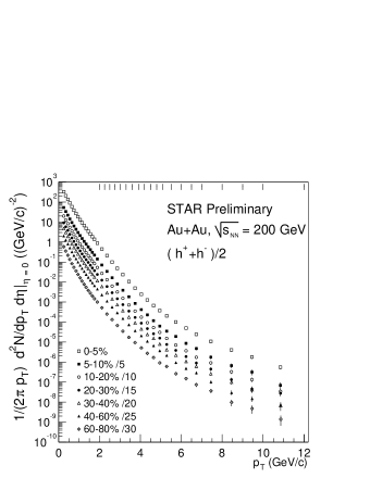
Figure 21: Transverse momentum spectra of charged hadrons in Au+Au collisions at $\sqrt{s}=200\>GeV$, in dependence of collision centrality 97 (offset as indicated), featuring transition from exponential to power law shape.

In order to infer from the spectral shapes of the hadronic species about the expansion mechanism, we first transform to the transverse mass variable, $m_{T}=(p^{2}_{T}+m^{2})^{1/2}$, via

$$\frac{1}{2\pi}\>\frac{dN_{i}}{p_{T}dp_{T}dy}=\frac{1}{2\pi}\>\frac{dN_{i}}{m_{T}dm_{T}dy}$$ (102)

because it has been shown in p+p collisions 98 near RHIC energy that the $m_{T}$ distributions of various hadronic species exhibit a universal pattern (”$m_{T}$ scaling”) at low $m_{T}$:

$$\frac{1}{2\pi}\>\frac{dN_{i}}{m_{T}dm_{T}dy}=A_{i}\>exp(-m^{i}_{T}/T)$$ (103)

with a universal inverse slope parameter $T$ and a species dependent normalization factor $A$. Hagedorn showed 99 that this scaling is characteristic of an adiabatic expansion of a fireball at temperature $T$. We recall that, on the other hand, an ideal hydrodynamical expansion is isentropic.

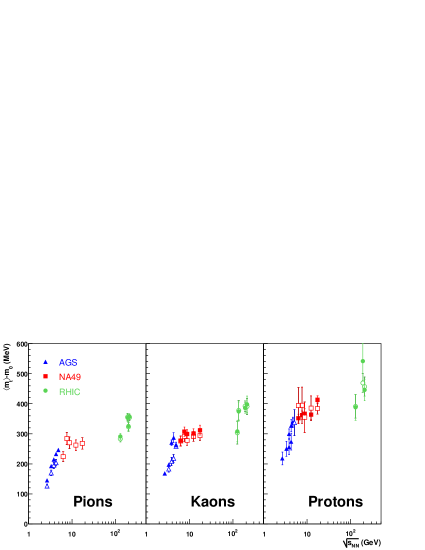
Figure 22: The average transverse kinetic energy $\left<m_{T}\right>-m_{0}$ for pions, kaons and protons vs. $\sqrt{s}$ in central Au+Au/Pb+Pb collisions 54 . Open symbols represent negative hadrons.

Fig. 22 shows the $\sqrt{s}$ dependence of the average transverse kinetic energy $\left<m^{i}_{T}\right>-m^{i}$ for pions, kaons and protons observed at mid-rapidity in central Au+Au/Pb+Pb collisions 54 . Similarly, the inverse slope parameter $T$ resulting from a fit of equation 103 to $K^{+}$ and $K^{-}$ transverse mass spectra (at $p_{T}\leq 2\>GeV/c$) is shown in Fig. 23, both for nuclear and p+p collisions 100 . We see, first of all, that $m_{T}$ scaling does not apply in A+A collisions, and that the kaon inverse slope parameter, $T\approx 230\>MeV$ over the SPS energy regime, can not be identified with the fireball temperature at hadron formation which is $T_{h}\approx 165\>MeV$ from Fig. 1. The latter is seen, however, to be well represented by the p+p spectral data exhibited in the left panel of Fig. 23. There is, thus, not only thermal energy present in A+A transverse expansion, but also hydrodynamical radial flow.

We note that the indications in Figs. 22 and 23, of a plateau in both $\left<m_{T}\right>$ and $T$, extending over the domain of SPS energies, $6\leq\sqrt{s}\leq 17\>GeV$, have not yet been explained by any fundamental expansive evolution model, including hydrodynamics. Within the framework of the latter model, this is a consequence of the initialization problem 96 which requires a detailed modeling, both of primordial energy density vs. equilibration time scale, and of the appropriate partonic matter equation of state (EOS) which relates expansion pressure to energy density. At top RHIC energy, this initialization of hydro-flow occurs, both, at a time scale $t_{0}\approx 0.5\>fm/c$ which is far smaller than the time scale of eventual bulk hadronization ($t\approx 3\>fm/c$), and at a primordial energy density far in excess of the critical QCD confinement density. After initialization, the partonic plasma phase thus dominates the overall expansive evolution,over a time interval far exceeding the formation and relaxation time scale.

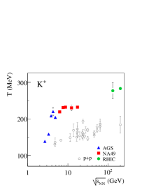
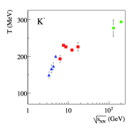
Figure 23: The inverse slope parameter $T$ of equation 103 for $K^{+}\mbox{and}\>K^{-}$ transverse mass spectra at $p_{T}<2\>GeV/c$ and mid-rapidity in central A+A, and in minimum bias p+p collisions 100 .

Thus, at RHIC energy, parton transport 92 and relativistic hydrodynamic 95 ; 96 models establish a well developed expansion mode that survives the subsequent stages of hadronization and hadronic expansion. This is reflected in their success in describing elliptic flow. On the other hand, the hydrodynamical model far overestimates elliptic flow at SPS energy 96 at which, as we have shown in section3.5, the initialization period may be not well separated from the confinement (hadronization) stage. Thus, whereas the expansion evolution at $\sqrt{s}=200\>GeV$ (occuring at near-zero baryo-chemical potential in Fig. 1) ”races” across the parton-hadron phase boundary with fully established flow patterns, near $\mu_{B}=0$ where lattice QCD predicts the phase transformation to be merely a soft cross-over 16 , the dynamics at $\sqrt{s}=10-20\>GeV$ may originate from only slightly above, or even at the phase boundary, thus sampling the domain $200\leq\mu_{B}\leq 500\>MeV$ where the equation of state might exhibit a ”softest point” 96 . The hydrodynamic model thus faces formidable uncertainties regarding initialization at SPS energy.

The plateau in Figs. 22, 23 may be the consequence of the fact that not much flow is generated in, or transmitted from the partonic phase, at SPS energies, because it is initialized close to the phase boundary 100 where the expected critical point 9 ; 10 (Fig. 1), and the corresponding adjacent first order phase transition might focus 101 or stall 96 the expansion trajectory, such that the observed radial flow stems almost exclusively from the hadronic expansion phase. The SPS plateau, which we shall subsequently encounter in other bulk hadron variables (elliptic flow, HBT radii) might thus emerge as a consequence of the critical point or, in general, of the flatness of the parton-hadron coexistence line. RHIC dynamics, on the other hand, originates from far above this line.

Hadronic expansion is known to proceed isentropically 102 : commensurate to expansive volume increase the momentum space volume must decrease, from a random isotropic thermal distribution to a restricted momentum orientation preferentially perpendicular to the fireball surface, i.e. radial. The initial thermal energy, implied by the hadron formation temperature $T_{H}=165\>MeV$, will thus fall down to a residual $T_{F}$ at hadronic decoupling from the flow field (”thermal freeze-out”) plus a radial transverse kinetic energy term $m_{i}\left<\beta_{T}\right>^{2}$ where $m_{i}$ is the mass of the considered hadron species and $\left<\beta_{T}\right>$ the average radial velocity. We thus expect 103 for the slope of equation 103:

$$T=T_{F}+m_{i}\left<\beta_{T}\right>^{2},\>p_{T}\leq 2\>GeV/c$$ (104)

and

$$T=T_{F}\left(\frac{1+\left<v_{T}\right>}{1-\left<v_{T}\right>}\right)^{1/2},\>p_{T}\gg m_{i}$$ (105)

the latter expression valid at $p_{T}$ larger than hadron mass scale ($T$ then is the ”blue-shifted temperature” at decoupling 104 and $\left<v_{T}\right>$ the average transverse velocity). The assumption that radial flow mostly originates from the hadronic expansion phase is underlined by the proportionality of flow energy to hadron mass (equation 104).

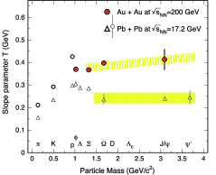
Figure 24: Hadron slope parameters $T$ at mid-rapidity as a function of mass. For Pb+Pb at $\sqrt{s}=17.3\>GeV$ (triangles) and Au+Au at $\sqrt{s}=200\>GeV$ (circles); from 103 .

Fig. 24 illustrates this proportionality, by a recent compilation 103 of RHIC results for central Au+Au collisions at $\sqrt{s}=200\>GeV$, and SPS results for central Pb+Pb collisions at top SPS energy, $\sqrt{s}=17.3\>GeV$. At the latter energy the slope parameter of the $\Phi$ meson is seen to be close to that of the similar mass baryons $p$ and $\Lambda$, emphasizing the occurence of $m_{i}$ scaling as opposed to valence quark number scaling that we will encounter in RHIC elliptic flow data 94 . As is obvious from Fig. 24 the multi-strange hyperons and charmonia exhibit a slope saturation which is usually explained 103 as a consequence of their small total cross sections of rescattering from other hadrons, leading to an early decoupling from the bulk hadron radial flow field, such that $\left<\beta_{T}\right>_{\Omega}\><\>\left<\beta_{T}\right>_{p}$.

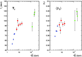
Figure 25: Hadron decoupling temperature $T_{f}$, and average radial flow velocity $\left<\beta_{T}\right>$ extracted from blast wave model (see equation 106) fits of $m_{T}$ spectra vs. $\sqrt{s}$ 54 .

According to our observations with equation 104 a hydrodynamical ansatz for the transverse mass spectrum of hadrons should thus contain the variables ”true temperature” $T_{F}$ at decoupling from the flow field, and its average velocity $\left<\beta_{T}\right>$, common to all hadrons. This is the case for the blast wave model 104 developed as an approximation to the full hydrodynamic formalism 96 , assuming a common decoupling or ”freeze-out” from flow, for all hadronic species, and a boost-invariant longitudinal expansion:

$$\frac{dN_{i}}{m_{T}dm_{T}dy}=A_{i}\>m_{T}\>K_{1}\>\left(\frac{m_{T}cosh\rho}{T_{F}}\right)\>I_{0}\left(\frac{p_{T}sinh\rho}{T_{F}}\right)$$ (106)

where $\rho=tanh^{-1}\beta_{T}$. In an extended version of this model a function is included that describes the radial profile of the transverse velocity field, $\beta_{T}(r)=\beta_{T}^{max}\>r/R$, instead of employing a fixed $\beta_{T}$ at decoupling 106 . Fig. 25 shows 54 the resulting energy dependence of $T_{F}$ and $\left<\beta_{T}\right>$, for the same set of data as implied already in Figs. 22 and 23. The ”true” decoupling temperature rises steeply at the AGS and less so at SPS energy (as does $\left<\beta_{T}\right>$), to a value of about $95\>MeV$ at top SPS energy, which is considerably lower than the chemical freeze-out temperature, $T_{H}=165\>MeV$, at which the hadronic species relative yield composition of the hadronic phase becomes stationary (see section 4, and Fig. 1). Chemical decoupling thus occurs early, near the parton-hadron phase boundary, whereas hadronic radial flow ceases after significant further expansion and cooling, whence the surface radial velocity (its average value given by $\left<\beta_{T}\right>$ in Fig. 25) approaches $\beta_{T}\approx 0.65$. Both data sets again exhibit an indication of saturation, over the interval toward top SPS energy: the SPS plateau. This supports our above conjecture that radial flow is, predominantly, a consequence of isentropic bulk hadronic expansion in this energy domain, which sets in at $T_{H}$. At RHIC energy, both parameters exhibit a further rise, suggesting that primordial partonic flow begins to contribute significantly to radial flow.

In summary we conclude that hadronic hadro-chemical freeze-out occurs near the parton-hadron boundary line of Fig. 1, at high $\sqrt{s}$. This fixes the hadronic species equilibrium distribution at $T=T_{H}$. Onward from hadronic freeze-out, the expanding system is out of equilibrium as far as its hadronic species composition is concerned. However the momentum space distributions are subject to further change during the hadronic expansion phase, predominantly due to elastic scattering and development of radial flow. This process ends in final decoupling from strong interaction, at $T_{f}<T_{H}$. Analysis of $p_{T}$ spectra exhibits a collective radial flow pattern at $T_{f}$, as characterized by a radial flow velocity $\beta_{T}$.

4 Hadronization and hadronic freeze-out in A+A collisions

Within the course of the global expansion of the primordial reaction volume the local flow ”cells” will hit the parton-hadron phase boundary as their energy density approaches $\epsilon_{crit}\approx 1\>GeV/fm^{3}$. Hadronization will thus occur, not at an instant over the entire interaction volume, but within a finite overall time interval 86 that results from the spread of proper time at which individual cells, or coherent clusters of such cells (as developed during expansion) arrive at the phase boundary. However, irrespective of such a local-temporal occurence, the hadronization process (which is governed by non perturbative QCD at the low $Q^{2}$ corresponding to bulk hadronization) universally results in a novel, global equilibrium property that concerns the relative abundance of produced hadrons and resonances. This so-called ”hadrochemical equilibrium state” is directly observable, in contrast to the stages of primordial parton equilibration that are only indirectly assessed, via dynamical model studies.

This equilibrium population of species occurs both in elementary and nuclear collisions 107 . We have seen in Fig. 19 a first illustration, by $e^{+}e^{-}$ annihilation data at $\sqrt{s}=91.2\>GeV$ LEP energy, that are well reproduced by the partition functions of the statistical hadronization model (SHM) in its canonical form 84 . The derived hadronization temperature, $T_{H}=165\>MeV$, turns out to be universal to all elementary and nuclear collision processes at $\sqrt{s}\geq 20\>GeV$, and it agrees with the limiting temperature predicted by Hagedorn 38 to occur in any multi-hadronic equilibrium system once the energy density approaches about $0.6\>GeV/fm^{3}$. Thus, the upper limit of hadronic equilibrium density corresponds, closely, to the lower limit, $\epsilon_{crit}=0.6-1.0\>GeV/fm^{3}$ of partonic equilibrium matter, according to lattice QCD 48 . In elementary collisions only about 20 partons or hadrons participate: there should be no chance to approach thermodynamic equilibrium of species by rescattering cascades, neither in the partonic nor in the hadronic phase. The fact that, nevertheless, the hadron formation temperature $T_{H}$ coincides with the Hagedorn limiting temperature and with the QCD confinement temperature, is a consequence of the non-perturbative QCD hadronization process itself 85 , which ”gives birth” to hadrons/resonances in canonical equilibrium, at high $\sqrt{s}$, as we shall see below. This process also governs A+A collisions but, as it occurs here under conditions of high energy density extended over considerable volume, the SHM description now requires a grand canonical ensemble, with important consequences for production of strange hadrons (strangeness enhancement).

The grand canonical order of hadron/resonance production in central A+A collisions, and its characteristic strangeness enhancement shows that a state of extended matter that is quantum mechanically coherent must exist at hadronization 87 ; 88 ; 107 . Whether or not it also reflects partonic equilibrium properties (including flavor equilibrium), that would allow us to claim the direct observation of a quark gluon plasma state near $T_{c}$, can not be decided on the basis of this observation alone, as the hadronization process somehow generates, by itself, the observed hadronic equilibrium. This conclusion, however, is still the subject of controversy 107 .

Figure 26: Total hadron multiplicities in central Pb+Pb collisions at $\sqrt{s}=17.3\>GeV$ 100 versus prediction of the grand canonical statistical hadronization model 19 .

Two typical examples of grand canonical SHM application are illustrated in Figs. 26 and 27, the first showing total hadron multiplicities in central Pb+Pb collisions at $\sqrt{s}=17.3\>GeV$ by NA49 100 confronted with SHM predictions by Becattini et al. 19 . This plot is similar to Fig. 19 in which $e^{+}e^{-}$ annihilation to hadrons is confronted with a SHM prediction derived from the canonical ensemble 84 . Central Au+Au collision data at $\sqrt{s}=200\>GeV$ from several RHIC experiments are compared to grand canonical model predictions by Braun-Munzinger et al. 108 in Fig. 27. The key model parameters, $T_{H}$ and the baryo-chemical potential $\mu_{B}$ result as $159\>MeV$ ($160\>MeV)$, and $247\>MeV$ ($20\>MeV)$ at $\sqrt{s}=17.3\>(200)\>GeV$, respectively. The universality of the hadronization temperature is obvious from comparison of the present values with the results of the canonical procedure employed in $e^{+}e^{-}$ annihilation to hadrons at $\sqrt{s}=91.2\>GeV$ (Fig. 19), and in canonical SHM fits 109 to p+p collision data at $\sqrt{s}=27.4\>GeV$ where $T_{H}=159$ and $169\>MeV$, respectively.

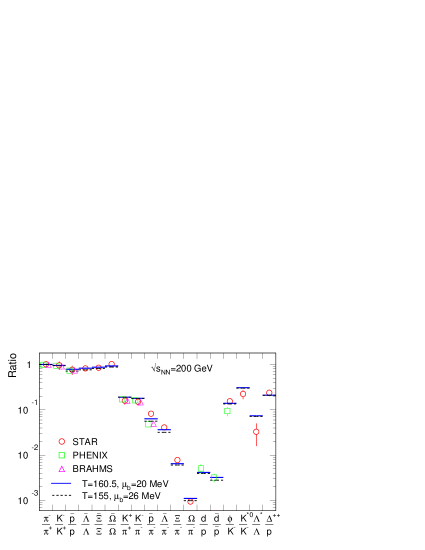
Figure 27: Hadron multiplicity ratios at mid-rapidity in central Au+Au collisions at $\sqrt{s}=200\>GeV$ from RHIC experiments STAR, PHENIX and BRAHMS, compared to predictions of the grand canonical statistical model 108 .

Figs. 26 and 27 illustrate two different approaches employed in grand canonical SHM application, the former addressing the values of the hadronic multiplicities as obtained in approximate full $4\pi$ acceptance (within limitations implied by detector performance), the latter employing a set of multiplicity ratios obtained in the vicinity of mid-rapidity as invited, at RHIC energy, by the limited acceptance of the STAR and PHENIX experiments. The latter approach is appropriate, clearly, in the limit of boost-invariant rapidity distributions where hadron production ratios would not depend on the choice of the observational rapidity interval. We have shown in section 3.2 that such conditions do, in fact, set in at top RHIC energy, as referred to in Fig. 27. However, at low $\sqrt{s}$ the y-distributions are far from boost-invariant, and the total rapidity gap $\Delta y$ may become comparable, in the extreme case, to the natural rapidity widths of hadrons emitted in the idealized situation of a single, isotropically decaying fireball positioned at mid-rapidity. Its rapidity spectra, equation 86, resemble Gaussians with widths $\Gamma_{i}\approx 2.35\>(T/m_{i})^{1/2}$ for hadron masses $m_{i}$. Clearly, the particle ratios $(dN_{i}/dy)/(dN_{j}/dy)$ then depend strongly on the position of the rapidity interval $dy$: away from $y=0$ heavy hadrons will be strongly suppressed, and particle yields in narrow rapidity intervals are useless for a statistical model analysis unless it is known a priori that the radiator is a single stationary spherical fireball 110 . This is not the case toward top SPS energy (see Fig. 12), due to significant primordial longitudinal expansion of the hadron emitting source. Given such conditions, the total multiplicity per collision event (the invariant yield divided by the total overall inelastic cross section) should be employed in the SHM analysis, as is exemplified in Fig. 26.

4.1 Hadronic freeze-out from expansion flow

The hadronic multiplicities result from integration of the invariant triple differential cross section over $p_{T}$ and $y$. Instrumental, experiment-specific conditions tend to result in incomplete $p_{T}$ and/or $y$ acceptances. It is important to ascertain that the effects of hydrodynamic transverse and longitudinal flow do not blast a significant part of the total hadron yield to outside the acceptance, and that they, more generally, do not change the relative hadron yield composition, thus basically affecting the SHM analysis. To see that hadronization incorporates only the internal energy in the co-moving frame 110 , we first assume that hadrochemical freeze-out occurs on a sharp hypersurface $\Sigma$, and write the total yield of particle species $i$ as

$$N_{i}=\int\frac{d^{3}p}{E}\int_{\Sigma}\>p^{\mu}d^{3}\sigma_{\mu}(x)\>f_{i}(x,p)=\int_{\Sigma}d^{3}\sigma_{\mu}(x)j_{i}^{\mu}(x)$$ (107)

where $d^{3}\sigma$ is the outward normal vector on the surface, and

$$j_{i}^{\mu}(x)=g_{i}\int d^{4}p2\Theta(p^{0})\delta(p^{2}-m^{2}_{i})\>p^{\mu}(exp\>[p\cdot u(x)-\mu_{i}]/T\pm 1)^{-1}$$ (108)

is the grand canonical number current density of species $i$, $\mu_{i}$ the chemical potential, $u(x)$ the local flow velocity, and $g_{i}$ the degeneracy factor. In thermal equilibrium it is given by

$$j_{i}^{\mu}(x) = \rho_{i}(x)u^{\mu}(x)\>\>\mbox{with}$$

$$\rho_{i}(x) = u_{\mu}(x)j_{i}^{\mu}(x)=\int d^{4}p2\Theta(p^{0})\delta(p^{2}-m_{i}^{2})\>p\cdot u(x)\>f_{i}(p\cdot u(x);T;\mu_{i})$$ (109)

$$= \int d^{3}p^{\prime}\>f_{i}(E_{p^{\prime}};T,\mu_{i})=\rho_{i}(T,\mu_{i}).$$

Here $E_{p^{\prime}}$ is the energy in the local rest frame at point $x$. The total particle yield of species $i$ is therefore

$$N_{i}=\rho_{i}(T,\mu_{i})\int_{\Sigma}d^{3}\sigma_{\mu}(x)u^{\mu}(x)=\rho_{i}(T,\mu_{i})\>V_{\Sigma}(u^{\mu})$$ (110)

where only the total comoving volume $V_{\Sigma}$ of the freeze-out hypersurface $\Sigma$ depends on the flow profile $u^{\mu}$. $V$ is thus a common total volume factor at hadronization (to be determined separately), and the flow pattern drops out from the yield distribution over species in $4\pi$ acceptance 110 . For nuclear collisions at SPS energies and below one thus should perform a SHM analysis of the total, $4\pi$-integrated hadronic multiplicities, as was done in Fig. 26.

We note that the derivation above illustrates the termination problem of the hydrodynamic description of A+A collisions, the validity of which depends on conditions of a short mean free path, $\lambda<1\>fm$. A precise argumentation suggests that two different free paths are relevant here, concerning hadron occupation number and hadron spectral freeze-out, respectively. As hadrochemical freeze-out occurs in the immediate vicinity of $T_{c}$ (and $T_{H}\approx 160-165\>MeV$ from Figs. 26, 27), the hadron species distribution stays constant throughout the ensuing hadronic phase, i.e the ”chemical” mean free path abruptly becomes infinite at $T_{H}$, whereas elastic and resonant rescattering may well extend far into the hadronic phase, and so does collective pressure and flow. In fact we have seen in section 3.6 that the decoupling from flow occurs at $T_{F}$ as low as $90-100\>MeV$ (Fig. 25). Thus the hydrodynamic evolution of high $\sqrt{s}$ collisions has to be, somehow artificially, stopped at the parton-hadron boundary in order to get the correct hadron multiplicities $N_{i}$, of equations 107 to 110, which then stay frozen-out during the subsequent hadronic expansion.

The equations (107-110) demonstrate the application of the Cooper-Frye prescription 111 for termination of the hydrodynamic evolution. The hyper-surface $\Sigma$ describes the space-time location at which individual flow cells arrive at the freeze-out conditions, $\epsilon=\epsilon_{c}$ and $T=T_{c}$, of hadronization. At this point, the resulting hadron/resonance spectra (for species $i$) are then given by the Cooper-Frye formula

$$E\frac{dN_{i}}{d^{3}p}=\frac{dN_{i}}{dyp_{T}dp_{T}}=\frac{g_{i}}{(2\pi)^{3}}\>\int_{\Sigma}f_{i}(p\cdot u(x),x)p\cdot d^{3}\sigma(x),$$ (111)

where $p^{\mu}f_{i}d^{3}\sigma_{\mu}$ is the local flux of particle $i$ with momentum $p$ through the surface $\Sigma$. For the phase space distribution $f$ in this formula one takes the local equilibrium distribution at hadronic species freeze-out from the grand canonical SHM

$$f_{i}(E,x)=[exp\{(E_{i}-\mu_{i}(x))/T\}\pm 1]^{-1}$$ (112)

boosted with the local flow velocity $u^{\mu}(x)$ to the global reference frame by the substitution $E\rightarrow p\cdot u(x)$. Fixing $T=T_{c}$ (taken e.g. from lattice QCD) the hadron multiplicities $N_{i}$ then follow from equation 110, and one compares to experiment, as in Figs. 26, 27. In order now to follow the further evolution, throughout the hadronic rescattering phase, and to finally compare predictions of equation 111 to the observed flow data as represented by the various Fourier-terms of equation 101 one has to re-initialize (with hadronic EOS) the expansion from $\Sigma$($T_{c}$ = 165 MeV) until final decoupling 96 , at $T\approx 100\>MeV$, thus describing e.g. radial and elliptic flow.

Alternatively, one might end the hydrodynamic description at $T=T_{c}$ and match the thus obtained phase space distribution of equation 111 to a microscopic hadron transport model of the hadronic expansion phase 95 ; 112 . This procedure is illustrated in Fig. 28 by an UrQMD 113 calculation of Bass and Dumitru 114 for central Au+Au collisions at top RHIC energy. We select here the results concerning the survival of the hadronic multiplicities $N_{i}$ throughout the dynamics of the hadronic expansion phase, which we have postulated above, based on the equality of the hadronization temperatures, $T_{H}\approx 160\>MeV$, observed in $e^{+}e^{-}$ annihilation (Fig. 19), where no hadronic expansion phase exists, and in central collisions of $A\approx 200$ nuclei (Figs. 26, 27). In fact, Fig. 28 shows that the $\{N_{i}\}$ observed at the end of the hadronic cascade evolution agree, closely, with the initial $\{N_{i}\}$ as derived from a Cooper-Frye procedure (equation 110) directly at hadronization. On the other hand, $p_{T}$ spectra and radial flow observables change, drastically, during the hadronic cascade expansion phase.

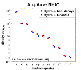
Figure 28: Modification of mid-rapidity hadron multiplicities in central Au+Au collisions at $\sqrt{s}=200\>GeV$ after chemical freeze-out at $T=T_{c}$. Squares show a hydrodynamic model prediction at $T=T_{c}$ (without further interaction); circles show the result of an attached UrQMD hadronic cascade expansion calculation 114 .

The hadronic multiplicity distribution $\{N_{i}\}$, arising from the hadronization process at high $\sqrt{s}$, freezes-out instantaneously also in A+A collisions, and is thus preserved throughout the (isentropic) hadronic expansion phase. It is thus directly measurable and, moreover, its hadrochemical equilibrium features lend themselves to an analysis within the framework of Hagedorn-type statistical, grand canonical models. As we shall show below, the outcome of this analysis is contained in a $[T_{H},\mu_{B}]$ parameter pair that reflects the conditions of QCD matter prevailing at hadronization, at each considered $\sqrt{s}$. In fact, the $[T,\mu]$ points resulting from the SHM analysis exhibited in Figs. 26, 27 (at $\sqrt{s}=17.3$ and $200\>GeV$, respectively) have been shown in the QCD matter phase diagram of Fig. 1 to approach, closely, the parton-hadron phase coexistence line predicted by lattice QCD. Thus, $T_{H}\approx T_{c}$ at high $\sqrt{s}$: hadrochemical freeze-out occurs in the immediate vicinity of QCD hadronization, thus providing for a location of the QCD phase boundary.

4.2 Grand canonical strangeness enhancement

The statistical model analysis 19 ; 107 ; 108 of the hadronization species distribution ${N_{i}}$ in A+A collisions is based on the grand canonical partition function for species $i$,

$$lnZ_{i}=\frac{g_{i}V}{6\pi^{2}T}\>\int^{\infty}_{0}\>\frac{k^{4}dk}{E_{i}(k)exp\left\{(E_{i}(k)-\mu_{i})/T\right\}\pm 1}$$ (113)

where $E_{i}^{2}=k^{2}+m^{2}_{i}$, and $\mu_{i}\equiv\mu_{B}B_{i}+\mu_{s}S_{i}+\mu_{I}I_{3}^{i}$ is the total chemical potential for baryon number $B$, strangeness $S$ and isospin 3-component $I_{3}$. Its role in equation 113 is to enforce, on average over the entire hadron source volume, the conservation of these quantum numbers. In fact, making use of overall strangeness neutrality $(\sum_{i}N_{i}S_{i}=0)$ as well as of conserved baryon number (participant Z+N) and isospin (participant (N-Z)/Z) one can reduce $\mu_{i}$ to a single effective potential $\mu_{b}$. Hadronic freeze-out is thus captured in three parameters, $T,V$ and $\mu_{b}$. The density of hadron/resonance species $i$ then results as

$$n_{i}=\frac{T}{V}\frac{\delta}{\delta_{\mu}}\>lnZ_{i}$$ (114)

which gives

$$N_{i}=Vn_{i}=\frac{g_{i}V}{(2\pi)^{2}}\>\int^{\infty}_{0}\frac{k^{2}dk}{exp\left\{(E_{i}(k)-\mu_{i})/T\right\}\pm 1}.$$ (115)

We see that the common freeze-out volume parameter is canceled if one considers hadron multiplicity ratios, $N_{i}/N_{j}$, as was done in Fig. 27. Integration over momentum yields the one-particle function

$$N_{i}=\frac{VTg_{i}}{2\pi^{2}}\>m_{i}^{2}\>\sum_{n=1}^{\infty}\>\frac{(\pm 1)^{n+1}}{n}\>K_{2}\left(\frac{nm_{i}}{T}\right)exp\left(\frac{n\mu_{i}}{T}\right)$$ (116)

where $K_{2}$ is the modified Bessel function. At high $T$ the effects of Bose or Fermi statistics (represented by the $\pm 1$ term in the denominators of equation 113 and equation 115) may be ignored , finally leading to the Boltzmann approximation

$$N_{i}=\frac{VTgi}{2\pi^{2}}\>m_{i}^{2}\>K_{2}\left(\frac{m_{i}}{T}\right)exp\left(\frac{\mu_{i}}{T}\right)$$ (117)

which is the first term of equation 116. This approximation is employed throughout the SHM analysis. It describes the primary yield of hadron species $i$, directly at hadronization. The abundance of hadronic resonance states is obtained convoluting equation 115 with a relativistic Breit-Wigner distribution 19 . Finally, the overall multiplicity, to be compared to the data, is determined as the sum of the primary multiplicity (cf. equation 117) and the contributions arising from the unresolved decay of heavier hadrons and resonances:

$$N_{i}^{observed}=N_{i}^{primary}+\sum_{j}Br(j\rightarrow i)\>N_{j}.$$ (118)

After having exposed the formal gear of grand canonical ensemble analysis we note that equation 117 permits a simple, first orientation concerning the relation of $T$ to $\mu_{B}$ in A+A collisions by considering, e.g., the antiproton to proton production ratio. From equation 117 we infer the simple expression

$$N(\overline{p})/N(p)=exp(-2\mu_{B}/T).$$ (119)

Taking the mid-rapidity value 0.8 for $\overline{p}/p$ (from Fig. 27) at top RHIC energy, and assuming that hadronization occurs directly at the QCD phase boundary, and hence $T\approx T_{c}\approx 165\>MeV$, we get $\mu_{B}\simeq 18\>MeV$ from equation 119, in close agreement with the result, $\mu_{B}=20\>MeV$, obtained 108 from the full SHM analysis. Equation 119 illustrates the role played by $\mu_{B}$ in the grand canonical ensemble. It logarithmically depends on the ratio of newly created quark-antiquark pairs (the latter represented by the $\bar{p}$ yield), to the total number of quarks including the net baryon number-carrying valence quarks (represented by the $p$ yield).

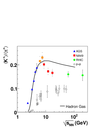
Figure 29: The ratio of total $K^{+}$ to total $\pi^{+}$ multiplicity as a function of $\sqrt{s}$, in central Au+Au and Pb+Pb collisions and in p+p minimum bias collisions 100 .

The most outstanding property of the hadronic multiplicities observed in central A+A collisions is the enhancement of all strange hadron species, by factors ranging from about 2 to 20, as compared to the corresponding production rates in elementary hadron-hadron (and $e^{+}e^{-}$ annihilation) reactions at the same $\sqrt{s}$. I.e. the nuclear collision modifies the relative strangeness output by a ”nuclear modification factor”, $R_{s}^{AA}=N_{s}^{AA}/0.5\>N_{part}\>\cdot\>N_{s}^{pp}$, which depends on $\sqrt{s}$ and $N_{part}$ and features a hierarchy with regard to the strangeness number $s=1,2,3$ of the considered species, $R^{AA}_{s=1}<R^{AA}_{s=2}<R^{AA}_{s=3}$. These properties are illustrated in Figs. 29 and 30. The former shows the ratio of total $K^{+}$ to positive pion multiplicities in central Au+Au/Pb+Pb collisions, from lower AGS to top RHIC energies, in comparison to corresponding ratios from minimum bias p+p collisions 100 . We have chosen this ratio, instead of $\left<K^{+}\right>/N_{part}$, because it reflects, rather directly, the ”Wroblewski ratio” of produced strange to non-strange quarks 107 , contained in the produced hadrons,

$$\lambda_{s}\equiv\frac{2(\left<s\right>+\left<\overline{s}\right>)}{\left<u\right>+\left<d\right>+\left<\overline{u}\right>+\left<\overline{d}\right>}\approx\begin{cases}0.2\ \text{in }\text{pp}\\ 0.45\ \text{in }\text{AA}.\end{cases}$$ (120)

The low value of $\lambda_{s}$ in $pp$ (and all other elementary) collisions reflects a quark population far away from $u,d,s$ flavor equilibrium, indicating strangeness suppression 109 .

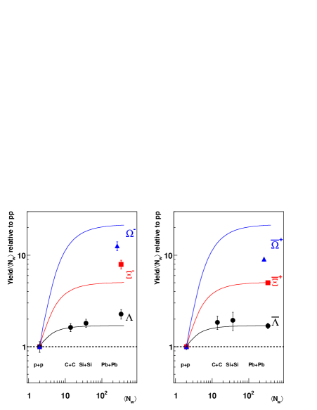
Figure 30: The nuclear modification factors $R^{AA}_{s=1,2,3}$ for hyperon and anti-hyperon production in nucleus-nucleus collisions at $\sqrt{s}=17.3\>GeV$, relative to the p+p reference at the same energy scaled by $N_{W}(=N_{part})$. The NA49 data refer to total $4\pi$ yields 116 . Closed lines represent the inverse strangeness suppression factors from ref. 119 , at this energy.

The so-called strangeness enhancement property of A+A collisions (obvious from Figs. 29 and 30) is, thus, seen as the removal of strangeness suppression; it is also referred to as a strangeness saturation, in SHM analysis 107 ; 108 , for the reason that $\lambda_{s}\approx 0.45$ corresponds to the grand canonical limit of strangeness production, implicit in the analysis illustrated in Figs. 26 and 27. The average $R^{AA}_{s=1}$ at $\sqrt{s}\geq 10\>GeV$ thus is about 2.2, both in the data of Fig. 29 and in the statistical model. It increases (Fig. 30) toward about 10 in s = 3 production of $\Omega$ hyperons.

In order to provide for a first guidance concerning the above facts and terminology regarding strangeness production we propose an extremely naive argument, based on the empirical fact of a universal hadronization temperature (Figs. 19, 26, 27) at high $\sqrt{s}$. Noting that $\left<s\right>=\left<\overline{s}\right>$ and $\left<u\right>\approx\left<\overline{u}\right>\approx\left<d\right>\approx\left<\overline{d}\right>$ in a QGP system at $\mu_{b}$ near zero, and $T=165\>MeV$, just prior to hadronization, $\lambda_{s}\approx\left<s\right>/\left<u\right>\approx exp\{(m_{u}-m_{s})/T\}=0.45$ at $p_{T}\rightarrow 0$ if we take current quark masses, $m_{s}-m_{u}\approx 130\>MeV$. I.e. the value of $\lambda_{s}$ in A+A collisions at high $\sqrt{s}$ resembles that of a grand canonical QGP at $\mu_{b}\rightarrow 0$, as was indeed shown in a 3 flavor lattice QCD calculation 115 at $T\approx T_{c}$. On the contrary, a p+p collision features no QGP but a small fireball volume, at $T\approx T_{c}$, within which local strangeness neutrality, $\left<s\right>=\left<\overline{s}\right>$ has to be strictly enforced, implying a canonical treatment 109 . In our naive model the exponential penalty factor thus contains twice the strangeness quark mass in the exponent, $\lambda_{s}\>\mbox{in pp collisions}\approx exp\{2(m_{u}-m_{s})/T\}\approx 0.2$, in agreement with the observations concerning strangeness suppression, which are thus referred to as canonical suppression. In a further extension of our toy model, now ignoring the $u,d$ masses in comparison to $m_{s}\approx 135\>MeV$, we can estimate the hierarchy of hyperon enhancement in A+A collisions,

$$R^{AA}_{s}\propto N_{s}^{AA}/N_{s}^{pp}\cdot 0.5\ N_{part}\approx exp\{(-sm_{s}+2sm_{s})/T\}=2.2,\>5.1,\>11.6$$ (121)

for $s=1,2,3$, respectively. Fig. 30 shows that these estimates correspond well with the data 116 for $R^{AA}$ derived in $4\pi$ acceptance for $\Lambda,\>\Xi\>\>\mbox{and}\>\>\Omega$ as well as for their antiparticles, from central Pb+Pb collisions at $\sqrt{s}=17.3\>GeV$. The p+p reference data, and C+C, Si+Si central collisions (obtained by fragmentation of the SPS Pb beam) refer to separate NA49 measurements at the same energy.

The above, qualitative considerations suggest that the relative strangeness yields reflect a transition concerning the fireball volume (that is formed in the course of a preceding dynamical evolution) once it enters hadronization. Within the small volumes, featured by elementary collisions (see section 4.3), phase space is severely reduced by the requirement of local quantum number conservation 109 ; 117 including, in particular, local strangeness neutrality. These constraints are seen to be removed in A+A collisions, in which extended volumes of high primordial energy density are formed. Entering the hadronization stage, after an evolution of expansive cooling, these extended volumes will decay to hadrons under conditions of global quantum mechanical coherence, resulting in quantum number conservation occuring, non-locally, and on average over the entire decaying volume. This large coherent volume decay mode removes the restrictions, implied by local quantum number balancing. In the above, naive model we have thus assumed that the hadronization of an Omega hyperon in A+A collisions faces the phase space penalty factor of only three $s$ quarks to be gathered, the corresponding three $\overline{s}$ quarks being taken care of elsewhere in the extended volume by global strangeness conservation. In the framework of the SHM this situation is represented by the grand canonical ensemble (equations 115, 117); the global chemical potential $\mu_{b}$ expresses quantum number conservation on average. Strict, local conservation is represented by the canonical ensemble.

The grand canonical (GC) situation can be shown to be the large collision volume limit (with high multiplicities $\{N_{i}\}$) of the canonical (C) formulation 118 ; 119 , with a continuous transition concerning the degree of canonical strangeness suppression 119 . To see this one starts from a system that is already in the GC limit with respect to baryon number and charge conservation whereas strangeness is treated canonically. Restricting to $s=1\>\>\mbox{and}\>\>-1$ the GC strange particle densities can be written (from equation 117) as

$$n_{s=\pm 1}^{GC}=\frac{Z_{s=\pm 1}}{V}\>\lambda^{\pm 1}_{s}$$ (122)

with

$$Z_{s=\pm 1}=\frac{Vg_{s}}{2\pi^{2}}\>m_{s}^{2}\>K_{2}\>(\frac{m_{s}}{T})\>exp\Big{\{}(B_{s}\mu_{B}+Q_{s}\mu_{Q})/T\Big{\}}$$ (123)

and a ”fugacity factor” $\lambda_{s}^{\pm 1}=exp\>(\mu_{s}/T)$. The canonical strange particle density can be written as 119

$$n_{s}^{C}=n_{s}^{GC}\cdot(\tilde{\lambda_{s}})$$ (124)

with an effective fugacity factor

$$\tilde{\lambda_{s}}\>=\>\frac{S_{\pm 1}}{\sqrt{S_{1}S_{-1}}}\>\frac{I_{1}(x)}{I_{0}(x)}$$ (125)

where $S_{\pm 1}=\sum_{s=\pm 1}\>Z_{s=\pm 1}$ is the sum over all created hadrons and resonances with $s=\pm 1$, the $I_{n}(x)$ are modified Bessel functions, and $x=2\sqrt{S_{1}S_{-1}}$ is proportional to the total fireball volume $V$. In the limit $x\approx V\rightarrow\infty$ the suppression factor $I_{1}(x)/I_{0}(x)\rightarrow 1$, and the ratio $S_{\pm 1}/\sqrt{S_{1}S_{-1}}$ corresponds exactly to the fugacity $\lambda_{s}$ in the GC formulation (see equation 122). Thus the C and GC formulations are equivalent in this limit, and the canonical strangeness suppression effect disappears. Upon generalization to the complete strange hadron spectrum, with $s=\pm 1,\pm 2,\pm 3,$ the strangeness suppression factor results 119 as

$$\eta(s)=I_{s}(x)/I_{0}(x).$$ (126)

In particular for small $x$ (volume), $\eta(s)\rightarrow(x/2)^{s}$, and one expects that the larger the strangeness content of the particle the smaller the suppression factor, and hence the larger the enhancement in going from elementary to central A+A collisions. This explains the hierarchy addressed in equation 121, and apparent from the data shown in Fig. 30. In fact, the curves shown in this figure represent the results obtained from equation 126, for $s=1,2,3$ hyperon production at $\sqrt{s}=17.3\>GeV$ 119 . They are seen to be in qualitative agreement with the data. However the scarcity of data, existing at top SPS energy for total hyperon yields, obtained in $4\pi$ acceptance (recall the arguments in section 4.1) both for A+A and p+p collisions does not yet permit to cover the SHM strangeness saturation curves in detail, for $s>1$.

This saturation is seen in Fig. 30, to set in already at modest system sizes, but sequentially so, for ascending hyperon strangeness. Note that SHM saturation is sequentially approached, from equation 126, with increasing fireball volume $V$. In order to make contact to the experimental size scaling with centrality, e.g. $N_{part}$, the model of ref. 119 , which is illustrated in Fig. 30, has converted the genuine volume scale to the $N_{part}$ scale by assuming a universal eigenvolume of $7\>fm^{3}$ per participant nucleon. I.e. $N_{part}=10$ really means a coherent fireball volume of $70\>fm^{3}$, in Fig. 30. Within this definition, saturation of $s=1,2,3$ sets in at fireball volumes at hadronization of about 60, 240 and 600 $fm^{3}$, respectively: this is the real message of the SHM curves in Fig. 30.

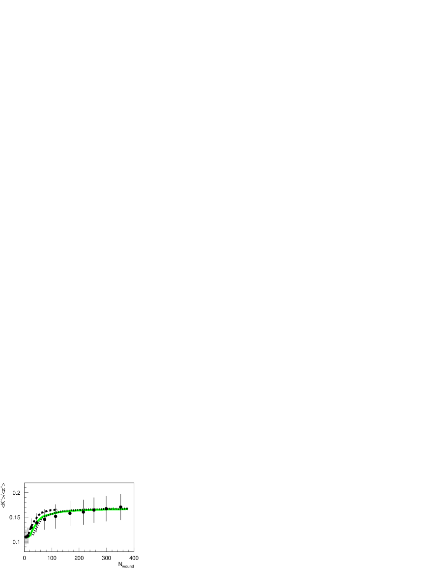
Figure 31: The mid-rapidity $K^{+}$ to $\pi^{+}$ ratio vs. $N_{part}$ in minimum bias Au+Au collisions at $\sqrt{s}=200\>GeV$, compared to the percolation model 120 (solid line); a prediction of which for Cu+Cu at similar energy is given by the long dashed line (see text for detail).

The above direct translation of coherent fireball volume to participant number is problematic 120 as it assumes that all participating nucleons enter into a single primordially coherent fireball. This is, however, not the case 120 particularly in the relative small scattering systems that cover the initial, steep increase of $\eta(s)$, where several local high density clusters are formed, each containing a fraction of $N_{part}$. This is revealed by a percolation model 120 of cluster overlapp attached to a Glauber calculation of the collision/energy density. At each $N_{part}$ an average cluster volume distribution results which can be transformed by equation 126 to an average $\{\eta(s,V)\}$ distribution whose weighted mean is the appropriate effective canonical suppression factor corresponding to $N_{part}$. On the latter scale, the SHM suppression curve thus shifts to higher $N_{part}$, as is shown in Fig. 31 for the $K^{+}/\pi^{+}$ ratio vs. $N_{part}$, measured at mid-rapidity by PHENIX in Au+Au collisions at $\sqrt{s}=200\>GeV$, which is reproduced by the percolation model 120 . Also included is a prediction for Cu+Cu at this energy which rises more steeply on the common $N_{part}$ scale because the collision and energy density reached in central Cu+Cu collisions, at $N_{part}\approx 100$, exceeds that in peripheral Au+Au collisions (at the same $N_{part}$) which share a more prominent contribution from the dilute surface regions of the nuclear density profile. We note, finally, that this deviation from universal $N_{part}$ scaling does not contradict the observations of a perfect such scaling as far as overall charged particle multiplicity densities are concerned (recall Fig. 15) which are dominated by pions, not subject to size dependent canonical suppression.

4.3 Origin of hadro-chemical equilibrium

The statistical hadronization model (SHM) is not a model of the QCD confinement process leading to hadrons, which occurs once the dynamical cooling evolution of the system arrives at $T_{c}$. At this stage the partonic reaction volume, small in elementary collisions but extended in A+A collisions, will decay (by whatever elementary QCD process) to on-shell hadrons and resonances. This coherent quantum mechanical decay results in a de-coherent quasi-classical, primordial on-shell hadron-resonance population which, at the instant of its formation, lends itself to a quasi-classical Gibbs ensemble description. Its detailed modalities (canonical for small decaying systems, grand canonical for extended fireballs in A+A collisions), and its derived parameters [$T,\mu_{B}$] merely recast the conditions, prevailing at hadronization. The success of SHM analysis thus implies that the QCD hadronization process ends in statistical equilibrium concerning the hadron-resonance species population.

In order to identify mechanisms in QCD hadronization that introduce the hadro-chemical equilibrium we refer to jet hadronization in $e^{+}e^{-}$ annihilation reactions, which we showed in Fig. 19 to be well described by the canonical SHM. In di-jet formation at LEP energy, $\sqrt{s}=92\>GeV$, we find a charged particle multiplicity of about 10 per jet, and we estimate that, likewise, about 10 primordial partons participate on either side of the back-to-back di-jet 85 . There is thus no chance for either a partonic or hadronic, extensive rescattering toward chemical equilibrium. However, in the jet hadronization models developed by Amati and Veneziano 83 , Webber 121 and Ellis and Geiger 85 the period of QCD DGLAP parton shower evolution (and of perturbative QCD, in general) ends with local color neutralization, by formation of spatial partonic singlet clusters. This QCD ”color pre-confinement” 83 process reminds of a coalescence mechanism, in which the momenta and the initial virtual masses of the individual clustering partons get converted to internal, invariant virtual mass of color neutral, spatially extended objects. Their mass spectrum 121 extends from about 0.5 to 10 $GeV$. This cluster mass distribution, shown in Fig. 32, represents the first stochastic element in this hadronization model.

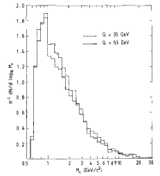
Figure 32: Invariant mass spectrum of color neutralization clusters in the Veneziano-Webber hadronization model 83 ; 121 .

The clusters are then re-interpreted within non-perturbative QCD: their internal, initially perturbative QCD vacuum energy gets replaced by non-perturbative quark and gluon condensates, making the clusters appear like hadronic resonances. Their subsequent quantum mechanical decay to on-shell hadrons is governed by the phase space weights given by the hadron and resonance spectrum 85 ; 121 . I.e. the clusters decay under ”phase space dominance” 85 , the outcome being a micro-canonical or a canonical hadron and resonance ensemble 84 ; 107 . The apparent hadro-chemical equilibrium thus is the consequence of QCD color neutralization to clusters, and their quantum mechanical decay under local quantum number conservation and phase space weights. We note that the alternative description of hadronization, by string decay 122 , contains a quantum mechanical tunneling mechanism, leading to a similar phase space dominance 123 .

Hadronization in $e^{+}e^{-}$ annihilation thus occurs from local clusters (or strings), isolated in vacuum, of different mass but similar energy density corresponding to QCD confinement. These clusters are boosted with respect to each other but it was shown 124 that for a Lorentz invariant scalar, such as multiplicity, the contributions of each cluster (at similar $T$) can be represented by a single canonical system with volume equal to the sum of clusters. In the fit of Fig. 19 this volume sum amounts to about 25 $fm^{3}$ 84 ; the individual cluster volumes are thus quite small, of magnitude a few $fm^{3}$ 85 . This implies maximum canonical strangeness suppression but may, in fact, require a micro-canonical treatment of strangeness 109 , implying a further suppression. These MC effects are oftentimes included 125 in the canonical partition functions by an extra strangeness fugacity parameter $\gamma_{s}<1$ which suppresses $s=1,2,3$ in a hierarchical manner, $\left<N_{i}(s)\right>\approx(\gamma_{s})^{s_{i}}$. The fit of Fig. 19 requires $\gamma_{s}=0.66$, a value typical of canonical multiplicity analysis in $p+p,\>p+\overline{p}$ and $e^{+}e^{-}$ annihilation collisions 109 at $\sqrt{s}\geq 30\>GeV$.

The above picture, of hadrochemical equilibrium resulting from the combined stochastic features of QCD color neutralization by cluster formation, and subsequent quantum mechanical decay to the on-shell hadron and resonance spectrum (under phase space governance) lends itself to a straight forward extension to A+A collisions. The essential new features, of grand canonical hadronization including strangeness enhancement, should result from the fact that extended space-time volumes of $\epsilon>\epsilon_{crit}$ are formed in the course of primordial partonic shower evolution, an overlap effect increasing both with $\sqrt{s}$ and with the size of the primordial interaction volume. As the volume of the elementary hadronization clusters amounts to several $fm^{3}$ it is inevitable that the clusters coalesce, to form extended ”super-cluster” volumes prior to hadronization 120 . As these super-clusters develop toward hadronization via non perturbative QCD dynamics, it is plausible to assume an overall quantum mechanical coherence to arise over the entire extended volume, which will thus decay to hadrons under global quantum number conservation, the decay products thus modeled by the GC ensemble.

Our expectation that space-time coalescence of individual hadronization clusters will lead to a global, quantum mechanically coherent extended super-cluster volume, that decays under phase space dominance, appears as an analogy to the dynamics and quantum mechanics governing low energy nuclear fission from a preceding “compound nucleus” 126 . Note that the observation of a smooth transition from canonical strangeness suppression to grand canonical saturation (Figs. 30, 31) lends further support to the above picture of a percolative growth 120 of the volume that is about to undergo hadronization.

An extended, coherent quark gluon plasma state would, of course, represent an ideal example of such a volume 127 and, in fact, we could imagine that the spatial extension of the plasma state results from a percolative overlap of primordial zones of high energy density, which becomes more prominent with increasing $\sqrt{s}$ and $N_{part}$. A QGP state preceding hadronization will thus lead to all the observed features. However, to be precise: the hadronizing QCD system of extended matter decaying quantum coherently, could still be a non-equilibrium precursor of the ideal equilibrium QGP, because we have seen above that hadrochemical equilibrium also occurs in $e^{+}e^{-}$ annihilation, where no partonic equilibrium exists. It gets established in the course of hadronization, irrespective of the degree of equilibrium prevailing in the preceding partonic phase.

4.4 Hadronization vs. rapidity and $\sqrt{s}$

We have argued in section 4.1 that, at relatively low $\sqrt{s}$, the total rapidity gap $\Delta y$ does not significantly exceed the natural thermal rapidity spreading width $\Gamma_{i}\approx 2.35\>(\Gamma/m_{i})^{1/2}$ of a single, isotropically decaying fireball, centered at mid-rapidity and emitting hadrons of mass $m_{i}$ 110 . However, this procedure involves an idealization because in the real Pb+Pb collision the intersecting dilute surface sections of the nuclear density profiles will lead to a significant contribution of single-scattering NN collisions, outside the central high density fireball. The leading hadron properties of such ”corona collisions” result in wider proper rapidity distributions, quite different from those of the central fireball decay hadrons. Their contribution will thus be prominent near target/projectile rapidity, and will feature a canonically suppressed strangeness. The one-fireball assumption, although inevitable at small $\Delta y$, does not quite resemble the physical reality. This may explain the need for an additional strangeness suppression factor in the GC one-particle partition function (equation 113) that has, unfortunately, also been labeled $\gamma_{s}$ but expresses physics reasons quite different from the extra suppression factor that reflects micro-canonical phase space constraints in elementary collisions. It turns out that all GC analysis of central A+A collisions at low $\sqrt{s}$, and addressed to total $4\pi$ multiplicities, requires a $\gamma_{s}$ of 0.7 - 0.85 19 ; in the fit of Fig. 26 $\gamma_{s}=0.84$.

At RHIC, $\Delta y\approx 11\gg\Gamma_{i}$, and such difficulties disappear: $\gamma_{s}\approx 1$ at midrapidity and, moreover, the wide gap permits a SHM analysis which is differential in $y$. Fig. 33 shows the $y$-dependence of the ratios $\pi^{-}/\pi^{+},\>K^{-}/K^{+}$ and $\overline{p}/p$ as obtained by BRAHMS 128 in central Au+Au collisions at $\sqrt{s}=200\>GeV$. The figure shows a dramatic dependence of the $\overline{p}/p$ ratio, which reflects the local baryochemical potential according to equation 119. At $y_{CM}>1$ the $\overline{p}/p$ ratio drops down steeply, to about 0.2 at $y\approx 3.5$, thus making close contact to the top SPS energy value obtained by NA49 129 . The $K^{-}/K^{+}$ ratio follows a similar but weaker drop-off pattern, to about 0.65 again matching with the top SPS energy value of about 0.6 130 . The deviation from unity of these ratios reflects the rapidity densities of initial valence $u,d$ quarks, relative to the densities of newly created light and strange quark-antiquark pairs, i.e. the $y$ distribution of the net baryon number density, and of the related baryo-chemical potential of the GC ensemble. Thus, in analyzing successive bins of the rapidity distributions in Fig. 33, the major variation in the GC fit concerns the baryo-chemical potential $\mu_{B}$(y) which increases from about 20 $MeV$ (Fig. 27) at mid-rapidity, to about 150 $MeV$ at $y\geq 3$ while the hadronization temperature stays constant, at $T=160\>MeV$. This interplay between $K^{-}/K^{+},\>\overline{p}/p$ and $\mu_{B}$ is illustrated 128 in the right hand panel of Fig. 33, and shown to be well accounted for by the GC statistical model 131 .

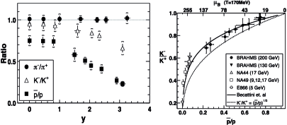
Figure 33: (left) Anti-hadron to hadron ratios as a function of rapidity in central Au+Au collisions at $\sqrt{s}=200\>GeV$. The right panel shows an interpretation of the correlation between $\overline{p}/p$ and $K^{-}/K^{+}$ in terms of baryo-chemical potential $\mu_{B}$ variation in the grand canonical statistical model. From 128 .

These considerations imply that hadronization at RHIC (and LHC) energy occurs local in $y$-space and late in time. The density distribution of net baryon number results from the primordial pQCD shower evolution (c.f. section 3.4), and is thus fixed at formation time, $t_{0}\leq 0.5\>fm/c$ at RHIC. Hadronization of the bulk partonic matter occurs later, at $t\geq 3\>fm/c$ 86 ; 95 , and transmits the local conditions in rapidity space by preserving the local net baryon quantum number density. Most importantly we conclude that hadronization occurs, not from a single longitudinally boosted fireball but from a succession of ”super-clusters”, of different partonic composition depending on $y$, and decaying at different time due to the Lorentz-boost that increases with $y$, in an ”inside-outside” pattern (c.f. Fig. 2). We are thus whitnessing at hadronization a Hubble expanding system of local fireballs. The detailed implications of this picture have not been analyzed yet. Note that a central RHIC collision thus does not correspond to a single hadronization ”point” in the [$T,\>\mu$] plane of Fig. 1 but samples $\{T,\>\mu\}$ along the QCD parton-hadron coexistence line 132 .

Throughout this section we have discussed hadronic freeze-out at high $\sqrt{s}$ only (top SPS to RHIC energy), because of the proximity of the chemical freeze-out parameters [$T,\>\mu_{b}$] to the QCD phase boundary from lattice QCD, which suggests an overall picture of hadronization, to occur directly from a partonic cluster or super-cluster. Our discussion of the GC statistical hadronization model has been explicitly or implicitly based on the assumption that hadronic freeze-out coincides with hadronization. However, the GC model has also been applied successfully to hadro-chemical freeze-out at $\sqrt{s}$ down to a few $GeV$ 19 ; 107 ; 108 where it is not expected that the dynamical evolution traverses the phase boundary at all, but grand canonical multiplicity distributions, and their characteristic strangeness enhancement pattern, are observed throughout. Toward lower $\sqrt{s},\>T$ decreases while $\mu_{b}$ increases, as is shown in Fig. 34 which presents a compilation of all reported freeze-out parameters 108 .

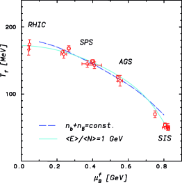
Figure 34: Energy dependence of the hadro-chemical freeze-out points obtained by grand canonical statistical model analysis in the plane [$T,\>\mu_{B}$], with interpolating curve at fixed energy per particle of about 1 $GeV$ 107 ; 139 .

These points have also been included in the phase diagram of Fig. 1 which shows that they are gradually branching away from the phase separation boundary line that could recently be predicted by lattice QCD once new methods had been developed to extend the theory to finite $\mu_{B}$ 9 ; 10 . At $\sqrt{s}\geq 20\>GeV$ we see that

$$\epsilon_{c}(QCD)\approx\epsilon_{H}\approx\epsilon_{GC}$$ (127)

where $\epsilon_{GC}$ is the freeze-out density inferred from GC analysis 19 ; 107 ; 108 .

In turn, the GC hadronic freeze-out points drop below the lattice QCD coexistence line at lower $\sqrt{s}$, implying that chemical freeze-out now occurs within the hadronic expansion phase. This requires a model of freeze-out, now governed by the properties of a high density hadronic medium, upon expansive cooling and dilution. Holding on to the model of a quantum mechanical de-coherence decay to on-shell hadrons that we discussed in section 4.3, we argue that an initial, extended high density hadronic fireball, given sufficient life-time at $T$ smaller, but not far below $T_{c}$, could also be seen as a quantum mechanically coherent super-cluster, as governed by effective mean fields 133 . In such a medium hadrons, at $T$ near $T_{c}$, acquire effective masses and/or decay widths far off their corresponding properties in vacuum: they are off-shell, approaching conditions of QCD chiral symmetry restoration as $T\rightarrow T_{c}$ 134 . This symmetry is inherent in the elementary QCD Langrangian, and ”softly” broken within the light quark sector by the small non-zero current quark masses, but severely broken at $T\rightarrow 0$ by the high effective constituent quark masses that get dressed by non perturbative QCD vacuum condensates. Pictorially speaking, hadrons gradually loose this dressing as $T\rightarrow T_{c}$ 135 , introducing a change, away from in vacuum properties, in the hadronic mass and width spectrum. Such in-medium chiral restoration effects have, in fact, been observed in relativistic A+A collisions, by means of reconstructing the in-medium decay of the $\rho$ vector meson to an observed $e^{+}e^{-}$ pair 136 .

A dense, high $T$ hadronic system, with mean-field induced off-shell constituents is also, clearly, quantum mechanically coherent. At a certain characteristic density, $\epsilon<\epsilon_{c}$, and temperature $T<T_{c}$, as reached in the course of overall hadronic expansion, this extended medium will undergo a decoherence transition to classical on-shell hadrons. Its frozen-out hadronic multiplicity distribution should be, again, characterized by the phase space weights of a grand canonical ensemble at $T<T_{c}$. Theoretical studies of such a mean field hadronic expansion mode 137 have also shown that such mechanisms play essentially no role at $\sqrt{s}\geq 20\>GeV$ because the expanding system is already in rapid flow once it traverses the phase boundary, with an expansion time scale shorter than the formation time scale of mean field phenomena. At lower energies, on the other hand, the system might not even dive into the deconfined phase but spend a comparatively long time in its direct vicinity, at the turning point between compression and re-expansion where all dynamical time constants are large, and the hadron density is high, such that the inelastic hadronic transmutation rate becomes high (particularly in collisions of more than two hadronic reactants, with reaction rates 138 proportional to $\epsilon^{n}$), and sufficiently so for maintaining hadronic chemical equilibrium after it is first established at maximum hadron density, in low $\sqrt{s}$ systems that do not cross the phase boundary at all.

The GC freeze-out parameters [$T,\mu$] at various $\sqrt{s}$ in Fig. 34 permit a smooth interpolation in the $T,\mu$ plane 139 , which, in turn, allows for GC model predictions which are continuous in $\sqrt{s}$. Such a curve is shown in Fig. 29 compared to the $4\pi$ data points for the $K^{+}/\pi^{+}$ multiplicity ratio in central collisions Au+Au/Pb+Pb, at all $\sqrt{s}$ investigated thus far. It exhibits a smooth maximum, due to the interplay of $T$ saturation and $\mu_{B}$ fall-off to zero, but does not account for the sharp peak structure seen in the data at $\sqrt{s}\approx 7\>GeV$ and $\mu_{B}\approx 480\>MeV$. This behavior is not a pecularity of the $K^{+}$ channel only; it also is reflected in an unusually high Wroblewski ratio (see equation 120) obtained at $\sqrt{s}=7.6\>GeV$, of $\lambda_{s}=0.60$ 19 . This sharp strangeness maximum is unexplained as of yet. It implies that hadron formation at this $\sqrt{s}$ reflects influences that are less prominent above and below, and most attempts to understand the effect 141 ; 142 ; 143 are centered at the assumption that at this particular $\sqrt{s}$ the overall bulk dynamics will settle directly at the phase boundary where, moreover, finite $\mu_{B}$ lattice theory also expects a QCD critical point 9 ; 10 ; 11 . This would cause a softest point to occur in the equation of state, i.e. a minimum in the relation of expansion pressure vs. energy density, slowing down the dynamical evolution 144 ; 145 , and thus increasing the sensitivity to expansion modes characteristic of a first order phase transition 143 , which occurs at $\mu_{b}\geq\mu_{b}^{crit}$. Such conditions may modify the K/$\pi$ ratio (Fig. 29) 143 .

It thus appears that the interval from top AGS to lower SPS energy, $5\leq\sqrt{s}\leq 10\>GeV$, promises highly interesting information regarding the QCD phase diagram (Fig. 1) in the direct vicinity of the parton-hadron coexistence line. In particular, the physics of a critical point of QCD matter deserves further study. Observable consequences also comprise so-called ”critical fluctuations” 146 ; 147 of multiplicity density, mean transverse momentum and hadron-chemical composition 148 , the latter in fact being observed near $\sqrt{s}=7\>GeV$ in an event by event study of the $K/\pi$ ratio in central Pb+Pb collisions 149 .

References

- (1) J. C. Collins and M. J. Perry, Phys. Rev. Lett. 34 (1975) 1353
-
(2)
E. V. Shuryak, Phys. Rept. 61 (1980) 71;
B. Müller, The Physics of the Quark-Gluon-Plasma, Springer Lecture Notes in Physics Vol.225, 1985;
L. McLerran, The Physics of the Quark-Gluon Plasma, Rev. Mod. Phys.58 (1986) 1012 - (3) S. Weinberg, The first three minutes, Basic Books Publ. 1977
- (4) R. Hagedorn, Suppl. Nuovo Cimento 3 (1965) 147
-
(5)
B. A. Freedman and L. McLerran, Phys. Rev. D16 (1977)
1169;
E. V. Shuryak, Zh. Eksp. Teor. Fiz.74 (1978) 408;
J. I. Kapusta, Nucl. Phys. B148 (1979) 461 - (6) L. Susskind, Phys. Rev. D20 (1979) 2610
- (7) J. Kuti, J. Polonyi and K. Szalachanyi, Phys. Lett. B98 (1981) 199
- (8) J. Engels, F. Karsch. I. Montvay and H. Satz, Phys. Lett. B101 (1981) 89
- (9) F. R. Brown, F. P. Butler, H. Chen, N. H. Christ, Z. Dong, W. Schaffer, L. I. Unger and A. Vaccarino, Phys. Rev. Lett. 65 (1990) 2491
- (10) F. Karsch, Nucl. Phys. A590 (1995) 372; R. Stock, hep-ph/9901415
-
(11)
Z. Fodor and S. D. Katz, JHEP 0203 (2002) 014;
Ph. de Forcrand and O. Philipsen, Nucl. Phys. B642 (2002) 290 - (12) C. R. Allton et al., Phys. Rev. D68 (2003) 014507
- (13) F. Karsch and E. Laerman, in Quark-Gluon Plasma 3, eds. R. C. Hwa and X. N. Wang, World Scientific 2004, p.1
- (14) S. L. Shapiro and S. Teukolsky, Black Holes, White Dwarfs and Neutron Stars, Wiley Publ., 1983
- (15) F. Weber, Pulsars as Astrophysical Laboratories, Inst. of Physics Publ., 1999
- (16) R. Oechslin, H. T. Janka and A. Marek, astro-ph/0611047
- (17) R. Rapp, T. Schäfer and E. V. Shuryak, Annals Phys. 280 (2000) 35
- (18) R. D. Pisarski and F. Wilczek, Phys. Rev. D29 (1984) 338
-
(19)
E. Witten, Phys. Rev. D30 (1984) 272;
H. Kurki-Suonio, R. A. Matzner, K.A. Olive and D. N. Schramm, Astrophys. J. 353 (1990) 406 - (20) K. Kajantie and H. Kurki-Suonio, Phys. Rev. D34 (1986) 1719
- (21) F. Becattini et al., Phys. Rev. C69 (2004) 024905
-
(22)
M. G. Alford, K. Rajagopal and F. Wilczek, Nucl. Phys.
B537 (1999) 443;
D. H. Rischke, Progr. Part. Nucl. Phys. 52 (2004) 197 - (23) J. P. Blaizot, E. Iancu and A. Rebhan, in Quark-Gluon Plasma 3, eds. R. C. Hwa and X. N. Wang, World Scientific 2004, p.60
-
(24)
G. Baym, B. L. Friman, J. P. Blaizot, M. Soyeur and W.
Czyz, Nucl. Phys. A407 (1983) 541;
H. Stöcker and W. Greiner, Phys. Rept. 137 (1986) 277;
L. P. Csernai, Introduction to relativistic heavy ion collisions, Wiley 1994;
P. Huovinen, P. F. Kolb and U. Heinz, Nucl. Phys. A698 (2002) 475 - (25) N. Cabibbo and G. Parisi, Phys. Lett. B59 (1975) 67
- (26) G. Veneziano, Nucl. Phys. B159 (1979) 213
-
(27)
G. T’Hooft, Nucl. Phys. B138 (1978) 1, and B190 (1981)
455;
A. Di Giacomo, Proc. Intern. School Enrico Fermi, Course 43, edit. A. Molinari and L. Riccati, IOS Press Anmsterdam 2003, p.401 - (28) B.B. Back et al.: The PHOBOS Perspectives on Discoveries at RHIC, Nuclear Physics A 757 (2005) 28
- (29) L. Van Hove: Phys. Lett. B 118, 138 (1982)
- (30) J. Gosset et al., Phys. Rev. C 16, 629 (1977)
- (31) T. Alber et al., NA49 Coll., Phys. Rev. Lett 75 (1995) 3814
- (32) M. Agarwal et al., WA98 Coll., Eur. Phys. J. C18 (2001) 651
- (33) F. Karsch, E. Laermann and A. Peikert, Nucl. Phys. B605 (2001) 579
- (34) J. D. Bjorken, Phys. Rev. D27 (1983) 140
- (35) J. Adams et al., STAR Coll., Nucl. Phys. A757 (2005) 102
-
(36)
K. J. Eskola, K. Kajantie, P. Ruuskanen and K.
Tuominen, Nucl. Phys. B570 (2000) 379;
E. V. Shuryak and L. Xiong, Phys. Rev. Lett. 70 (1993) 2241 -
(37)
M. D. Baker et al., PHOBOS Coll., Nucl. Phys. A715
(2003) 65;
P. A. Steinberg et al., PHOBOS Coll., ibidem p.490 -
(38)
F. Karsch, E. Laerman and A. Peikert, Phys. Lett. B478
(2000) 447;
S. Hands, Contemp. Phys. 42 (2001) 209 - (39) P. Abreu et al., Phys. Lett. B459 (1999) 597
- (40) M. Basile et al., Phys. Lett. B92 (1980) 367 and Phys. Lett. B95 (1980) 311
- (41) G. Panduri and C. Rubbia UA1 Coll., Nucl. Phys. A418 (1984) 117
- (42) G. Roland et al., PHOBOS Coll., Nucl. Phys. A774 (2006) 113
- (43) J. Jalilian-Marian, J. Phys. G30 (2004) 751
- (44) Ch. Blume, J. Phys. G31 (2005) 57, and references therein
-
(45)
L. D. Landau, Izv. Akad. Nauk. SSSR 17 (1953) 52;
P. Carruthers and M. Duong-Van, Phys. Rev. D8 (1973) 859 - (46) I. G. Baerden et al., BRAHMS Coll., Phys. Rev. Lett. 93 (2004) 102301, and references to the other data therein
- (47) Ch. Blume et al., NA49 Coll., nucl-ex/0701042
- (48) P. Drijard et al., Nucl. Phys. B155 (1979) 269
- (49) A. Bialas, M. Bleszynski and W. Czyz, Nucl. Phys. B111 (1976) 461
- (50) A. Bialas and W. Czyz, Acta Phys. Pol. 36 (2005) 905
- (51) M. Gyulassy and L. McLerran, Nucl. Phys. A750 (2005) 30
- (52) A. H. Müller, Nucl. Phys. A715 (2003) 20, and references therein
- (53) N. Armestro, C. A. Salgado and U. A. Wiedemann, Phys. Rev. Lett. 94 (2005) 022002
- (54) D. Kharzeev, E. Levin and M. Nardi, hep-ph/0408050
- (55) S. Afanasiev et al., NA49 Coll., Nucl. Instr. Meth. A430 (1999) 210
- (56) K. Werner, Phys. Rept. 232 (1993) 87
- (57) B. Lungwitz, NA49 Coll., Frankfurt Thesis 2004
- (58) L. D. McLerran and R. Venugopalan, Phys. Rev. D49 (1994) 2233 and ibid. 3352
- (59) U. V. Gribov, E. M. Levin and M. G. Ryskin, Phys. Rept. 100 (1983) 1
-
(60)
A. H. Müller J. Qiu, Nucl. Phys. B268 (1986) 427;
J. P. Blaizot and A. H. Müller, Nucl. Phys. B289 (1987) 847 - (61) J. Breitweg et al., Eur. Phys. J. 67 (1999) 609, and references therein
- (62) S. J. Brodsky, H. C. Pauli and S. S. Pinsky, Phys. Rept. 301 (1998) 299
- (63) R. K. Ellis, W. J. Stirling and B. R. Webber, QCD and Collider Physics, Cambridge Monographs 1996
- (64) For a review see E. Iancu and R. Venugopalan in Quark-Gluon Plasma 3, eds. R. C. Hwa and N. X. Wang, p. 249, World Scientific 2004
-
(65)
Y. L. Dokshitzer, Sov. Phys. JETP 46 (1977) 641;
G. Altarelli and G. Parisi, Nucl. Phys. B126 (1977) 298 - (66) D. Kharzeev, E. Levin and M. Nardi, hep-ph/0111315
-
(67)
A. M. Stasto, K. Golec-Biernat and J. Kwiecinski,
Phys. Rev. Lett. 86 (2001) 596;
K. Golec-Biernat and M. Wüsthoff, Phys. Rev. D59 (1999) 3006 -
(68)
C. Adloff et al., Eur. Phys. J. C21 (2001) 33;
J. Breitweg et al., Phys. Lett. B487 (2000) 53 -
(69)
M. R. Adams et al., Z. Phys. C67 (1995) 403;
M. Arneodo et al., Nucl. Phys. B481 (1996) 3 and 23 - (70) R. Baier, A. H. Müller and D. Schiff, hep-ph/0403201, and references therein
- (71) B. B. Back et al., PHOBOS Coll., Phys. Rev. C65 (2002) 061901; nucl-ex/0405027
- (72) D. Amati and G. Veneziano, Phys. Lett. B83 (1979) 87
- (73) F. Becattini, Nucl. Phys. A702 (2002) 336
- (74) J. Ellis and K. Geiger, Phys. Rev. D54 (1996) 1967
-
(75)
K. Geiger and B. Müller, Nucl. Phys. B369 (1992) 600;
K. Geiger and D. K. Shrivastava, Nucl. Phys. A661 (1999) 592 - (76) R. Stock, Phys. Lett. B456 (1999) 277
- (77) U. Heinz, Nucl. Phys. A610 (1996) 264
- (78) Y. M. Sinyukov, Nucl. Phys. A498 (1989) 151
- (79) H. Appelshäuser et al., NA49 Coll., Eur. Phys. J. C2 (1998) 611
- (80) J. Rafelski and B. Müller, Phys. Rev. Lett. 48 (1982) 1066
- (81) D. Molnar and M. Gyulassy, Nucl. Phys. A697 (2002) 495, and Nucl. Phys. A698 (2002) 379
-
(82)
S. A. Voloshin and A. M. Poskanzer, Phys. Lett. B474
(2000) 27;
S. A. Voloshin, Nucl. Phys. A715 (2003) 379 - (83) R. A. Lacey and A. Taranenko, nucl-ex/0610029
- (84) D. Teaney, J. Laurent and E. V. Shuryak, Nucl. Phys. A698 (2002) 479, and nucl-th/0110037
- (85) J. L. Klay et al., STAR Coll., Nucl. Phys. A715 (2003) 733
- (86) K. Alpgard et al., Phys. Lett. B107 (1981) 310
- (87) R. Hagedorn and J. Ranft, Nuovo Cim. Suppl. 6 (1968) 169
-
(88)
M. Gazdzicki et al., NA49 Coll., J. Phys. G30 (2004)
701;
M. Gazdzicki et al., Braz. Journal of Physics 34 (2004) 322 - (89) P. F. Kolb and U. Heinz, in Quark-Gluon Plasma 3, edit. R. C. Hwa and Y. N. Wang, World Scientific 2004, p. 634, and references therein
- (90) C. Nonaka and M. Asakawa, Phys. Rev. C71 (2005) 044904
- (91) G. Bertsch and P. Cuguon, Phys. Rev. C24 (1981) 269
- (92) N. Xu, J. Phys. G32 (2006) 123, and references therein
- (93) E. Schnedermann, J. Sollfrank and U. Heinz, Phys. Rev. C48 (1993) 2462
- (94) U. Wiedemann and U. Heinz, Phys. Rev. C56 (1997) 3265
-
(95)
R. Stock, nucl-th/0703050;
P. Braun-Munzinger, K. Redlich and J. Stachel, in Quark-Gluon Plasma 3, eds. R. C. Hwa and X. N. Wang, World Scientific 2004, p. 491 - (96) A. Andronic, P. Braun-Munzinger and J. Stachel, nucl-th/0511071
- (97) F. Becattini and U. Heinz, Z. Phys. C76 (1997) 269
- (98) U. Heinz, nucl-th/9810056
- (99) F. Cooper and G. Frye, Phys. Rev. D10 (1974) 186
- (100) H. Sorge, Z. Phys. C67 (1995) 479
- (101) M. Bleicher et al., J. Phys. G25 (1999) 1859
- (102) S. A. Bass and A. Dimitru, Phys. Rev. C61 (2000) 064909
- (103) M. Mitrovski et al., NA49 Coll., J. Phys. G32 (2006) 43
- (104) A. Tounsi and K. Redlich, J. Phys. G28 (2002) 2095
- (105) R. V. Gavai and S. Gupta, J. Phys. G30 (2004) 1333
- (106) E. V. Shuryak, Phys. Lett. B42 (1972) 357
- (107) J. Rafelski and M. Danos, Phys. Lett. B97 (1980) 279
- (108) C. Hoehne, F. Puehlhofer and R. Stock, Phys. Lett. B640 (2006) 96
- (109) B. R. Webber, Nucl. Phys. B238 (1984) 492
- (110) B. Andersson, G. Gustafsson, G. Ingelman and T. Sjöstrand, Phys. Rept. 97 (1983) 33
- (111) H. Satz, hep-ph/0612151; P. Castorina, D. Kharzeev and H. Satz, hep-ph/0704.1426
- (112) F. Becattini and G. Passaleva, Eur. Phys. Journ. C23 (2002) 551
- (113) J. Rafelski, Phys. Lett. B262 (1991) 333
- (114) W. S. C. Williams, Nuclear and Particle Physics, Oxford Univ. Press 1991
- (115) B. Müller and J. Rafelski, Phys. Rev. Lett. 48 (1982) 1066
- (116) I. G. Baerden et al., BRAHMS Coll., Phys. Rev. Lett. 90 (2003)102301
- (117) C. Alt et al., NA49 Coll., Phys. Rev. C73 (2006) 044910
- (118) S. V. Afanasiev et al., NA49 Coll., Phys. Rev. C69 (2004) 024902
- (119) F. Becattini et al., Phys. Rev. C64 (2001) 024901
- (120) D. Röhrich, Florenz
- (121) P. Braun-Munzinger, J. Cleymans, H. Oeschler and K. Redlich, Nucl. Phys. A697 (2002) 902
- (122) R. Rapp, J. Phys. G31 (2005) 217
- (123) G. E. Brown and M. Rho, Phys. Rept. 269 (1996) 333
- (124) R. Rapp and J. Wambach, Adv. Nucl. Phys. 25 (2000) 1
- (125) S. Damjanovic et al., NA60 Coll., Nucl. Phys. A774 (2006) 715
- (126) D. Zschiesche et al., Nucl. Phys. A681 (2001) 34
- (127) C. Greiner et al., J. Phys. G31 (2005) 61
- (128) M. Gazdzicki and M. I. Gorenstein, Acta Phys. Polon B30 (1999) 2705
- (129) R. Stock, J. Phys. G30 (2004) 633
- (130) V. Koch, A. Majumder and J. Randrup, nucl-th/0509030
- (131) E. G. Nikonow, A. A. Shanenko and V. D. Toneev, Heavy Ion Physics 8 (1998) 89
-
(132)
C. M. Hung and E. V. Shuryak, Phys. Rev. C57 (1998)
1891;
M. Bleicher, hep-ph/0509314 - (133) M. Stephanov, K. Rajagopal and E. V. Shuryak, Phys. Rev. Lett. 81 (1998) 4816
- (134) M. Stephanov, K. Rajagopal and E. V. Shuryak, Phys. Rev. D60 (1999) 114028
- (135) V. Koch, A. Majumder and J. Randrup, nucl-th/0505052
- (136) Ch. Roland et al., NA49 Coll., J. Phys. G30 (2004) 1371