Discussion on some characteristics of the Charged Brane-world Black holes

Abstract

Several physical natures of charged brane-world black holes have been investigated. At first, time-like and null geodesics of the charged brane-world black holes are presented. We also analyze all the possible motions by plotting the effective potentials for various parameters for circular and radial geodesics. Secondly, we investigate the motion of test particles in the gravitational field of charged brane-world black holes using Hamilton-Jacobi ( H-J ) formalism. We have considered charged and uncharged test particles and examine its behavior both in static and non-static cases. Thirdly, thermodynamics of the charged brane-world black holes are studied. Finally, it has been also shown that there is no phenomenon of superradiance for an incident massless scalar field for this black hole.

1. Introduction

In recent, scientists have given their attention to brane world gravity. In brane world models, the ordinary matter fields are confined on a three dimensional subspace, called brane embedded in 1+3+d dimensions in which the gravity can propagate in the d-extra dimensions. Here, the d-extra dimensions need not all be small or even compact. Most of the recent studies consider a simple version of the brane world scenario where all matters ( except gravity ) are confined to a 3-brane embedded in a five dimensional space-time ( bulk ) while gravity can propagate in the bulk. Recently, Dadhich et. al [1] have presented a spherically symmetric solution which describes a black hole localized on a three brane in five dimensional gravity in the brane world scenario. This black hole ( without electric charge ) is termed as tidal charged black hole. In this case, tidal charge is arising via gravitational effects from the fifth dimension i.e. it is arising from the projection on to the brane of free gravitational field effects in the bulk. Chamblin et. al [2] studied charged brane world black holes in Randall and Sundrum model. In this model, they assumed our universe as a domain wall in asymtotically anti-de Sitter space. This type of black holes can have two types of ”charge”, one comes from the bulk Weyl tensor and the other from a gauge field trapped on the wall. By using the brane-world Einstein equations, a $Reissner-Norstr\ddot{o}m$ (RN) geometry can be found on the domain wall provided that only the bulk Weyl charge is present [3]. Chamblin et. al showed that the extent of the horizon in the fifth dimension for a charged black hole is usually less than for an uncharge black hole that has the same mass or the same horizon radius on the wall.

In this paper, we will discuss the behavior of the time-like and null geodesics of the charged brane-world black holes.We will analyze all the possible motions by plotting the effective potentials for various parameters for circular and radial geodesics. Also we will investigate the motion of test particles in the gravitational field of charged brane-world black holes using Hamilton-Jacobi method. We have considered charged and uncharged test particles and examine its behaviour both in static and non-static cases. Thermodynamics of the charged brane-world black holes are studied. It has been also checked that if there is any phenomenon of superradiance or not for an incident massless scalar field for this black hole.

2. Charged Brane-World Black holes metric

A Charged Brane-World Black holes metric can be written as[2]

$$ds^{2}=-f(r)dt^{2}+\frac{dr^{2}}{f(r)}+r^{2}(d\theta^{2}+sin^{2}\theta d\phi^{2})$$ (1)

where

$$f(r)=1-\frac{2GM}{r}+\frac{Q^{2}+\beta}{r^{2}}+\frac{l^{2}Q^{4}}{20r^{6}}$$

M,Q and $\beta$ corresponds to Mass,electro-magnetic charge and tidal charge of the black hole respectively.
The electric gauge potential have the form $A_{i}=-\Phi(r)dt$ with $\Phi(r)=\frac{Q}{r}$.

3. The Geodesics

Let us now write down the equation for the geodesics in the metric (1) . From

$$\frac{d^{2}x^{\mu}}{d\tau^{2}}+\Gamma^{\mu}_{\nu\lambda}\frac{dx^{\nu}}{d\tau}\frac{dx^{\lambda}}{d\tau}=0$$ (2)

we have

$$\frac{1}{f(r)}\left(\frac{dr}{d\tau}\right)^{2}=\frac{E^{2}}{f(r)}-\frac{J^{2}}{r^{2}}-L$$ (3)

$$r^{2}\left(\frac{d\phi}{d\tau}\right)=J$$ (4)

$$\frac{dt}{d\tau}=\frac{E}{f(r)}$$ (5)

where the motion is considered in the $\theta=\frac{\pi}{2}$ plane and constants E and J are identified as the energy per unit mass and angular momentum, respectively , about an axis perpendicular to the invariant plane $\theta=\frac{\pi}{2}$. Here $\tau$ is the affine parameter and L is the Lagrangian having values 0 and 1, respectively, for massless and massive particles.
The equation for radial geodesic ( $J=0$):

$$\dot{r}^{2}\equiv\left(\frac{dr}{d\tau}\right)^{2}=E^{2}-Lf(r)$$ (6)

Using eqn.(5) and eqn.(3) we get

$$\left(\frac{dr}{dt}\right)^{2}=\left(1-\frac{2GM}{r}+\frac{Q^{2}+\beta}{r^{2}}+\frac{l^{2}Q^{4}}{20r^{6}}\right)^{2}\left[1-\frac{L}{E^{2}}\left(1-\frac{2GM}{r}+\frac{Q^{2}+\beta}{r^{2}}+\frac{l^{2}Q^{4}}{20r^{6}}\right)\right]$$ (7)

3.1 Motion of Massless Particle ( L=0 )

In this case,

$$\left(\frac{dr}{dt}\right)^{2}=\left(1-\frac{2GM}{r}+\frac{Q^{2}+\beta}{r^{2}}+\frac{l^{2}Q^{4}}{20r^{6}}\right)^{2}$$ (8)

Neglecting the higher order of $(Q^{2}+\beta)$ , $l^{2}Q^{4}$ , $GM$ and after integrating, we get the $t-r$ relationship as

$\pm t=r+2GMlnr+\frac{Q^{2}+\beta}{r}+\frac{l^{2}Q^{4}}{100r^{5}}-\frac{4G^{2}M^{2}}{r}-\frac{(Q^{2}+\beta)^{2}}{3r^{3}}-\frac{l^{4}Q^{8}}{4400r^{11}}+\frac{GM(Q^{2}+\beta)}{r^{2}}-\frac{l^{2}Q^{4}(Q^{2}+\linebreak\beta)}{70r^{7}}+\frac{GMl^{2}Q^{4}}{30r^{6}}$ .

The $t-r$ relationship is depicted in Fig. 1.

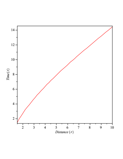
Figure 1: $t-r$ relationship for massless particle( choosing $G=M=Q=l=1$, $\beta=1$ )

Again, from equation (6) we get

$$\dot{r}^{2}\equiv\left(\frac{dr}{d\tau}\right)^{2}=E^{2}$$ (9)

After integrating, we get the $\tau-r$ relationship as

$$\pm E\tau=r$$ (10)

We show graphically (see Fig. 2 ) the variation of proper-time ($\tau$) with respect to radial co-ordinates (r) .

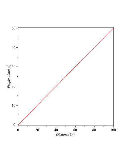
Figure 2: $\tau-r$ relationship for massless particle ( choosing $E=2$ )

3.2 Motion of Massive Particles ( L=1 )

In this case,

$$\left(\frac{dr}{dt}\right)^{2}=\left(1-\frac{2GM}{r}+\frac{Q^{2}+\beta}{r^{2}}+\frac{l^{2}Q^{4}}{20r^{6}}\right)^{2}.\frac{1}{E^{2}}\left(E^{2}-1+\frac{2GM}{r}-\frac{Q^{2}+\beta}{r^{2}}-\frac{l^{2}Q^{4}}{20r^{6}}\right)$$ (11)

After integrating, we get

$$\pm t=\int\frac{Edr}{\left(1-\frac{2GM}{r}+\frac{Q^{2}+\beta}{r^{2}}+\frac{l^{2}Q^{4}}{20r^{6}}\right)\sqrt{E^{2}-1+\frac{2GM}{r}-\frac{Q^{2}+\beta}{r^{2}}-\frac{l^{2}Q^{4}}{20r^{6}}}}$$ (12)

This gives the $t-r$ relationship as (neglecting the higher order of $(Q^{2}+\beta)$ and $l^{2}Q^{4}$)
(see graphical Fig. (3))

$\pm t=\frac{E}{\sqrt{E^{2}-1}}[r+\left(2GM-\frac{GM}{E^{2}-1}\right)lnr-\left(4G^{2}M^{2}-(Q^{2}+\beta)+\frac{Q^{2}+\beta}{2(E^{2}-1)}+\frac{3}{2}\frac{G^{2}M^{2}}{(E^{2}-1)^{2}}-\frac{2G^{2}M^{2}}{E^{2}-1}\right)\frac{1}{r}\linebreak-\frac{1}{r^{2}}(4G^{3}M^{3}-2GM(Q^{2}+\beta)-\frac{3}{4}\frac{GM(Q^{2}+\beta)}{(E^{2}-1)^{2}}-\frac{5}{4}\frac{G^{3}M^{3}}{(E^{2}-1)^{3}}+GM(\frac{Q^{2}+\beta}{2(E^{2}-1)}+\frac{3}{2}\frac{G^{2}M^{2}}{(E^{2}-1)^{2}})-\frac{GM}{E^{2}-1}(4G^{2}M^{2}-(Q^{2}+\beta)))+..............]$

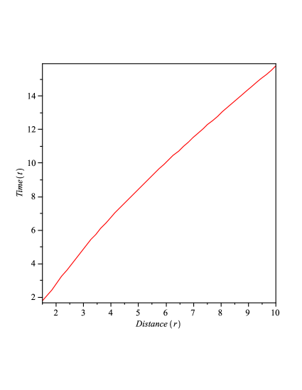
Figure 3: $t-r$ relationship for massive particle( choosing $G=M=Q=l=1,E=2$, $\beta=1$ )

Again, from equation (6) we get

$$\dot{r}^{2}\equiv\left(\frac{dr}{d\tau}\right)^{2}=E^{2}-\left(1-\frac{2GM}{r}+\frac{Q^{2}+\beta}{r^{2}}+\frac{l^{2}Q^{4}}{20r^{6}}\right)$$

After simplification, we get

$$\pm\int d\tau=\int\frac{dr}{\sqrt{E^{2}-\left(1-\frac{2GM}{r}+\frac{Q^{2}+\beta}{r^{2}}+\frac{l^{2}Q^{4}}{20r^{6}}\right)}}$$

Neglecting the higher order of $(Q^{2}+\beta)$ and $l^{2}Q^{4}$ gives the $\tau-r$ relationship as

$\pm\tau=\frac{1}{\sqrt{E^{2}-1}}[r-\frac{GM}{E^{2}-1}lnr-\left(\frac{Q^{2}+\beta}{2(E^{2}-1)}+\frac{3G^{2}M^{2}}{(E^{2}-1)^{2}}\right)\frac{1}{r}+\frac{3}{4}\frac{GM(Q^{2}+\beta)}{(E^{2}-1)^{2}}\frac{1}{r^{2}}-\frac{(Q^{2}+\beta)^{2}}{8(E^{2}-1)^{2}}\frac{1}{r^{3}}\linebreak-\frac{l^{2}Q^{4}}{200(E^{2}-1)}\frac{1}{r^{5}}+\frac{GMl^{2}Q^{4}}{80(E^{2}-1)^{2}}\frac{1}{r^{6}}-\frac{3l^{2}Q^{4}(Q^{2}+\beta)}{560(E^{2}-1)^{2}}\frac{1}{r^{7}}-\frac{3l^{4}Q^{8}}{35200(E^{2}-1)^{2}}\frac{1}{r^{11}}]$

We show graphically (see Fig. 4 ) the variation of proper-time ($\tau$) with respect to radial co-ordinates (r) .

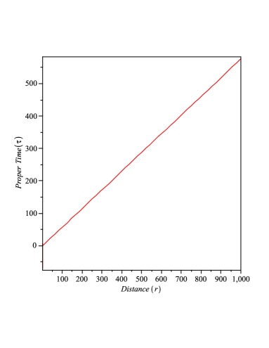
Figure 4: $\tau-r$ relationship for massive particle ( choosing $G=M=Q=l=1$, $\beta=1$ and $E=2$ )

4. EFFECTIVE POTENTIAL

From the Geodesic equation (3),(4) and (5) we can write

$$\frac{1}{2}\left(\frac{dr}{d\tau}\right)^{2}=\frac{1}{2}\left[E^{2}-f(r)\left(\frac{J^{2}}{r^{2}}+L\right)\right]$$ (13)

Comparing eqn.(13) with $\frac{\dot{r}^{2}}{2}+V_{eff}=0$, one can get the effective potential,which depends on E and L as follows :

$$V_{eff}=-\frac{1}{2}\left[E^{2}-f(r)\left(\frac{J^{2}}{r^{2}}+L\right)\right]$$ (14)

4.1 For Massless Particle ( L=0 )

At first consider, at the radial geodesics where J=0. The corresponding $V_{eff}$ is given by

$$V_{eff}=-\frac{E^{2}}{2}$$

If, $E=0$, then $V_{eff}=0$ i.e. the particle behaves like a ”free particle”. The graph of $V_{eff}$ for $E\neq 0$ is shown in Fig. 5. It is obvious that the behaviour of these geodesics is independent on the charge and mass of the black hole.

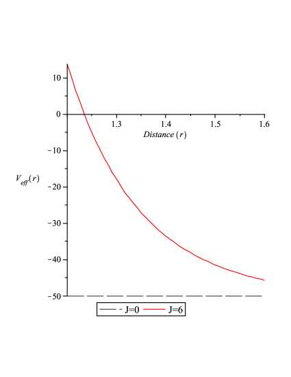
Figure 5: The effective potential for photons for M=2,G=1,$\beta=1$,$Q=\sqrt{2},l^{2}=80$,E=10.

Now consider, for circular geodesics where $J\neq 0$. The corresponding effective potential is,

$$V_{eff}=-\frac{E^{2}}{2}+\frac{J^{2}}{2r^{2}}\left(1-\frac{2GM}{r}+\frac{Q^{2}+\beta}{r^{2}}+\frac{l^{2}Q^{4}}{20r^{6}}\right)$$ (15)

For $r\rightarrow 0$, the effective potential,$V_{eff}(r)$ is very large and approaches $-\frac{E^{2}}{2}$ when $r\rightarrow\infty$. At the horizons, $V_{eff}=-\frac{E^{2}}{2}$. Let us consider, the effective potential for $E=0$ [put E=0 in eqn.(15)]. The roots of the potential coincide with the horizon values for this case. The potential is negative between the horizons. Hence, the particle would be bounded between the horizons. Again, since potential has a minimum between the horizons, stable circular orbits do exists. Fig.6 is an example for such a case.

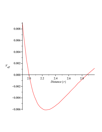
Figure 6: The effective potential for photons for M=2,G=1,$\beta=1$,$Q=\sqrt{2},l^{2}=80$,J=1.

Furthermore, there will be three sign changes in the $V_{eff}$. Hence, there will be at most three positive roots for $V_{eff}$. If we put E=0, then according to Descarte’s rule of signs, the effective potential has at most two positive roots.

4.2 For Massive Particle ( L=1 )

The corresponding potential is given by,

$$V_{eff}=-\frac{E^{2}}{2}+\frac{1}{2}f(r)\left(1+\frac{J^{2}}{r^{2}}\right)$$ (16)

where $f(r)=\left(1-\frac{2GM}{r}+\frac{Q^{2}+\beta}{r^{2}}+\frac{l^{2}Q^{4}}{20r^{6}}\right).$

It is to be mentioned that the roots of $f(r)$ are the horizons. First, consider for radial geodesics with J = 0. As $f(r)>0$ in the region $0\leq r<r_{-}$, $V_{eff}$ will vanish for some finite value of r in that region. Therefore, a time-like geodesic will not reach the singularity. The massive particle will avoid the singularity and would emerge in other regions. The space-time is geodesically complete. We can analyze the various cases of motion as follows: If we take E=0, then $V_{eff}$ becomes

$$V_{eff}=\frac{1}{2}\left(1-\frac{2GM}{r}+\frac{Q^{2}+\beta}{r^{2}}+\frac{l^{2}Q^{4}}{20r^{6}}\right)$$ (17)

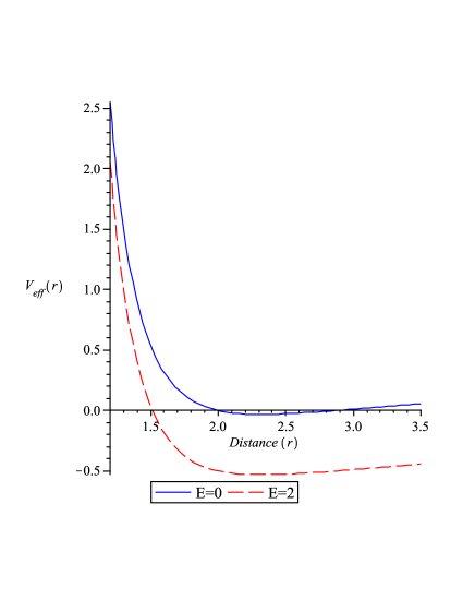
Figure 7: The effective potential (for radial geodesic) for massive particles for M=2,G=1,$\beta=1$,$Q=\sqrt{2},l^{2}=80$.

The zeros of the $V_{eff}$ coincide with the horizons. An example of such a case is shown in Fig.7 .

From the shape of the potential, it is clear that the particle can move only inside the black hole. Secondly, one can investigate the behaviour of $V_{eff}$ for $E\neq 0$. The corresponding $V_{eff}$ is given by eqn.(16). In this case, for $r\rightarrow 0$ the effective potential becomes

$$V_{eff}\rightarrow\frac{l^{2}Q^{4}}{20r^{6}}+\frac{Q^{2}+\beta}{r^{2}}-\frac{2GM}{r}$$

For large r, $V_{eff}\rightarrow\frac{1-E^{2}}{2}$. For a black hole with two horizons, in the two ranges, $0\leq r<r_{-}$ and $r_{+}<r$, the function $f(r)>0$. Hence it is possible for $V_{eff}$ to have roots in those two regions. Examples for two roots are given in Fig.7.
Now we will consider the particles with angular momentum ( $J\neq 0$). For E=0, the roots of the potential coincides with the two horizons and the shape of the $V_{eff}$ is given in Fig. 8. Hence the massive particle with ”zero energy” would not escape the black hole and would describe bounded orbits. The particle could have circular stable orbits since the potential has a minimum.

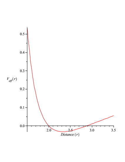
Figure 8: The effective potential for massive particles for M=2,G=1,$\beta=1$,$Q=\sqrt{2},l^{2}=80$,J=1.

Now for $E\neq 0$, $V_{eff}\rightarrow\frac{1-E^{2}}{2}$ for large r.

For $r\rightarrow 0$,

$$V_{eff}\rightarrow\frac{J^{2}}{2r^{2}}\left(1-\frac{2GM}{r}+\frac{Q^{2}+\beta}{r^{2}}+\frac{l^{2}Q^{4}}{20r^{6}}\right).$$

Similar to the arguments given for radial geodesics, it is possible for $V_{eff}$ to have finite roots in the regions $0\leq r<r_{-}$ and $r_{+}<r$. $V_{eff}$ will have two or three roots due to it’s behaviour around $r=0$. In both the cases a massive particle would describe bounded orbits.

An example is shown in Fig.8 for two root cases. The two horizons lie inside the region of the two roots of the potential. Hence the particle will describe elliptic orbits. There is a minimum for the potential as visible from Fig.8. Therefore it is possible for a particle to have a stable circular orbit inside the black hole.

5. Motion of test particle

Let us consider a test particle having mass,$m_{0}$ and charge, $e$ moving in the gravitational field of the Charged Brane-world black hole described by the metric ansatz(1). So the Hamilton-Jacobi [ H-J ] equation for the test particle is [4]

$$g^{ik}\left(\frac{\partial S}{\partial x^{i}}+eA_{i}\right)\left(\frac{\partial S}{\partial x^{k}}+eA_{k}\right)+m_{0}^{2}=0$$

where $g_{ik}$, $A_{i}$(gauge potential) are the classical background fields (1) and S is the standard Hamilton’s characteristic function.

For the metric (1) the explicit form of H-J equation is [5]

$$-\frac{1}{f}\left(\frac{\partial S}{\partial t}+\frac{eQ}{r}\right)^{2}+f\left(\frac{\partial S}{\partial r}\right)^{2}+\frac{1}{r^{2}}\left(\frac{\partial S}{\partial\theta}\right)^{2}+\frac{1}{r^{2}\sin^{2}\theta}\left(\frac{\partial S}{\partial\phi}\right)^{2}+m_{0}^{2}=0$$ (18)

In order to solve this partial differential equation, let us choose the $H-J$ function $S$ as [5]

$$S(t,r,\theta,\phi)=-E.t+S_{1}(r)+S_{2}(\theta)+{J.\phi}$$

where $E$ is identified as the energy of the particle and $J$ is the angular momentum of the particle.

The radial velocity of the particle is ( for detailed calculations, see $ref.[6]$ )

$$\frac{dr}{dt}=f^{2}\left(E-\frac{eQ}{r^{2}}\right)^{-1}\sqrt{\frac{1}{f^{2}}\left(E-\frac{eQ}{r}\right)^{2}-\frac{m_{0}^{2}}{f}-\frac{p^{2}}{fr^{2}}}$$ (19)

where $p$ is the separation constant and termed as momentum of the particle.

The turning points of the trajectory are given by $\left(\frac{dr}{dt}\right)=0$ and we get

$$\left(E-\frac{eQ}{r}\right)^{2}-m_{0}^{2}f-\frac{p^{2}}{r^{2}}f=0$$

Solving

$$E=\frac{eQ}{r}+\sqrt{f}\left(m_{0}^{2}+\frac{p^{2}}{r^{2}}\right)^{1/2}$$

The potential curve is given by

$$V(r)\equiv\frac{E}{m_{0}}=\frac{eQ}{m_{0}r}+\sqrt{f}\left(1+\frac{p^{2}}{m_{0}^{2}r^{2}}\right)^{1/2}$$

i.e.

$$V(r)=\frac{eQ}{m_{0}r}+\left(1+\frac{p^{2}}{m_{0}^{2}r^{2}}\right)^{1/2}\sqrt{1-\frac{2GM}{r}+\frac{Q^{2}+\beta}{r^{2}}+\frac{l^{2}Q^{4}}{20r^{6}}}$$

In a stationary system, $E$ i.e. $V(r)$ must have an extremal value. Hence the value of $r$ for which energy attains the extremal value is given by the equation

$$\frac{dV}{dr}=0$$ (20)

which gives

$$\frac{dV}{dr}=-\frac{eQ}{m_{0}r^{2}}+\frac{1}{2\sqrt{f}}\left(1+\frac{p^{2}}{m_{0}^{2}r^{2}}\right)^{1/2}f^{\prime}(r)-\sqrt{f}\left(1+\frac{p^{2}}{m_{0}^{2}r^{2}}\right)^{-1/2}\frac{p^{2}}{m_{0}^{2}r^{3}}=0$$

We obtain

$$\frac{eQ}{m_{0}r^{2}}\sqrt{f}\left(1+\frac{p^{2}}{m_{0}^{2}r^{2}}\right)^{1/2}=\frac{1}{2}\left(1+\frac{p^{2}}{m_{0}^{2}r^{2}}\right)f^{\prime}(r)-f\frac{p^{2}}{m_{0}^{2}r^{3}}$$

Putting the expression of $f$ we obtain

$$\begin{split}\frac{eQ}{m_{0}}\left(1-\frac{2GM}{r}+\right.&\left.\frac{Q^{2}+\beta}{r^{2}}+\frac{l^{2}Q^{4}}{20r^{6}}\right)^{1/2}\left(1+\frac{p^{2}}{m_{0}^{2}r^{2}}\right)^{1/2}=\\ &\left(GM-\frac{Q^{2}+\beta}{r}-\frac{3}{20}\frac{l^{2}Q^{4}}{r^{5}}\right)\left(1+\frac{p^{2}}{m_{0}^{2}r^{2}}\right)-\frac{p^{2}}{m_{0}^{2}r}\left(1-\frac{2GM}{r}+\frac{Q^{2}+\beta}{r^{2}}+\frac{l^{2}Q^{4}}{20r^{6}}\right)\end{split}$$ (21)

5.1 Test particle in Static Equilibrium

In static equilibrium, momentum $p$ must be zero. So, the value of $r$ for which potential will be an extremal is given by

$$\frac{eQ}{m_{0}}\left(1-\frac{2GM}{r}+\frac{Q^{2}+\beta}{r^{2}}+\frac{l^{2}Q^{4}}{20r^{6}}\right)^{1/2}=\left(GM-\frac{Q^{2}+\beta}{r}-\frac{3}{20}\frac{l^{2}Q^{4}}{r^{5}}\right)$$

From this, we get

$$\begin{split}\left(G^{2}M^{2}-\frac{e^{2}Q^{2}}{m_{0}^{2}}\right)r^{10}&+2GM\left[\frac{e^{2}Q^{2}}{m_{0}^{2}}-(Q^{2}+\beta)\right]r^{9}+(Q^{2}+\beta)\left[(Q^{2}+\beta)-\frac{e^{2}Q^{2}}{m_{0}^{2}}\right]r^{8}\\ &-\frac{3}{10}GMl^{2}Q^{4}r^{5}+l^{2}Q^{4}\left[\frac{6(Q^{2}+\beta)}{m_{0}^{2}}-\frac{e^{2}Q^{2}}{20m_{0}^{2}}\right]r^{4}+\frac{9}{400}l^{2}Q^{8}=0\end{split}$$

If $\frac{e^{2}Q^{2}}{m_{0}^{2}}>G^{2}M^{2}$,we see that last term of the equation is negative. So this equation has at least one positive real root. Again, if $\frac{e^{2}Q^{2}}{m_{0}^{2}}=G^{2}M^{2}$ and $\frac{e^{2}Q^{2}}{m_{0}^{2}}<(Q^{2}+\beta)$, then the above equation changed to nine degree equation with negative last term implies a real positive root exists.Therefore, it is possible to have bound orbit for the test particle i.e. the test particle can be trapped by the charged Brane-world black hole. In other words, the charged Brane-world black hole exerts an attractive gravitational force towards matter.

5.2 Test particle in Non-Static Equilibrium

Case I : Uncharged test particle $(e=0)$

Now the expression (21) simplifies to

$$\left(\frac{GM}{r^{2}}-\frac{Q^{2}+\beta}{r^{3}}-\frac{3}{20}\frac{l^{2}Q^{4}}{r^{7}}\right)\left(1+\frac{p^{2}}{m_{0}^{2}r^{2}}\right)=\frac{p^{2}}{m_{0}^{2}r^{3}}\left(1-\frac{2GM}{r}+\frac{Q^{2}+\beta}{r^{2}}+\frac{l^{2}Q^{4}}{20r^{6}}\right)$$

Thus we get the following algebraic equation as

$$5m_{0}^{2}GMr^{7}-5m_{0}^{2}\left[(Q^{2}+\beta)+\frac{p^{2}}{m_{0}^{2}}\right]r^{6}+15p^{2}GMr^{5}-10p^{2}(Q^{2}+\beta)r^{4}-15l^{2}Q^{2}m_{0}^{2}r^{2}-p^{2}l^{2}Q^{4}=0$$ (22)

Obviously, this equation has at least one positive real root since the last term of the above expression is negative. So it is possible to have a bound orbit for the test particle.

Case II : Test particle with charge $(e\neq 0)$

From eqn.(21), we have the algebraic equation

$$\begin{split}\frac{eQ}{m_{0}r^{2}}&\left(1-\frac{2GM}{r}+\frac{Q^{2}+\beta}{r^{2}}+\frac{l^{2}Q^{4}}{20r^{6}}\right)^{1/2}\left(1+\frac{p^{2}}{m_{0}^{2}r^{2}}\right)^{1/2}\\ &=\left(\frac{GM}{r^{2}}-\frac{Q^{2}+\beta}{r^{3}}-\frac{3}{20}\frac{l^{2}Q^{4}}{r^{7}}\right)\left(1+\frac{p^{2}}{m_{0}^{2}r^{2}}\right)-\frac{p^{2}}{m_{0}^{2}r^{3}}\left(1-\frac{2GM}{r}+\frac{Q^{2}+\beta}{r^{2}}+\frac{l^{2}Q^{4}}{20r^{6}}\right)\end{split}$$

After simplifying the earlier eqn. we get

$$\begin{split}\left(G^{2}M^{2}-\frac{e^{2}Q^{2}}{m_{0}^{2}}\right)r^{14}&+2GM\left[\frac{e^{2}Q^{2}}{m_{0}^{2}}-(Q^{2}+\beta+\frac{p^{2}}{m_{0}^{2}})\right]r^{13}\\ &+\left[(Q^{2}+\beta+\frac{p^{2}}{m_{0}^{2}})^{2}+\frac{6p^{2}G^{2}M^{2}}{m_{0}^{2}}-\frac{e^{2}Q^{2}(Q^{2}+\beta)}{m_{0}^{2}}-\frac{e^{2}Q^{2}p^{2}}{m_{0}^{4}}\right]r^{12}\\ &+\left[\frac{2GMe^{2}p^{2}Q^{2}}{m_{0}^{4}}-\frac{6p^{2}GM(Q^{2}+\beta+\frac{p^{2}}{m_{0}^{2}})}{m_{0}^{2}}-\frac{4p^{2}GM(Q^{2}+\beta)}{m_{0}^{2}}\right]r^{11}\\ &+\left[\frac{9G^{2}M^{2}p^{4}}{m_{0}^{4}}+\frac{4p^{2}(Q^{2}+\beta)(Q^{2}+\beta+\frac{p^{2}}{m_{0}^{2}})}{m_{0}^{2}}-\frac{e^{2}p^{2}Q^{2}(Q^{2}+\beta)}{m_{0}^{4}}\right]r^{10}\\ &-\left[\frac{3GMl^{2}Q^{4}}{10}+\frac{12p^{4}GMQ^{2}(Q^{2}+\beta)}{m_{0}^{4}}\right]r^{9}\\ &+\left[\frac{4p^{4}(Q^{2}+\beta)^{2}}{m_{0}^{4}}+\frac{6l^{2}Q^{4}(Q^{2}+\beta+\frac{p^{2}}{m_{0}^{2}})}{m_{0}^{2}}-\frac{e^{2}l^{2}Q^{6}}{20m_{0}^{2}}\right]r^{8}-\frac{13p^{2}GMl^{2}Q^{4}}{20m_{0}^{2}}r^{7}\\ &+\left[-\frac{e^{2}l^{2}p^{2}Q^{6}}{20m_{0}^{4}}+\frac{2p^{2}l^{2}Q^{4}(Q^{2}+\beta+\frac{p^{2}}{m_{0}^{2}})}{5m_{0}^{2}}+\frac{12p^{2}l^{2}Q^{4}(Q^{2}+\beta)}{20m_{0}^{2}}\right]r^{6}\\ &-\frac{6GMl^{2}p^{4}Q^{4}}{5m_{0}^{4}}r^{5}+\left[\frac{9l^{2}Q^{8}}{400}+\frac{4p^{4}l^{2}Q^{4}(Q^{2}+\beta)}{5m_{0}^{4}}\right]r^{4}+\frac{6p^{2}l^{2}Q^{8}}{100m_{0}^{2}}r^{2}+\frac{p^{4}l^{4}Q^{8}}{25m_{0}^{4}}=0\end{split}$$

If $\frac{e^{2}Q^{2}}{m_{0}^{2}}>G^{2}M^{2}$,we see that last term of the equation is negative. So this equation has at least one positive real root. Again,if $\frac{e^{2}Q^{2}}{m_{0}^{2}}=G^{2}M^{2}$ and $\frac{e^{2}Q^{2}}{m_{0}^{2}}<(Q^{2}+\beta+\frac{p^{2}}{m_{0}^{2}})$, then the above equation changed to thirteen degree equation with negative last term implies a real positive root exists.Therefore, it is possible to have bound orbit for the test particle i.e. the test particle can be trapped by the charged Brane-world black hole. In other words, the charged Brane-world black hole exerts an attractive gravitational force towards matter in this case also.

6. Thermodynamics

For a static black hole, Hawking temperature $T_{H}$ is an important thermodynamical quantity. For the Charged brane-world black hole metric $T_{H}$ is given by

$$T_{H}=\frac{1}{\sqrt{-g_{tt}g_{rr}}}\frac{d}{dr}(-g_{tt})\mid_{r=r_{h}}$$

Now $g_{tt}=f(r)=0$ yields ( See details in Annexure )

$$r^{3}+a_{1}r^{2}+a_{2}r+a_{3}=0$$ (23)

where $a_{1}=-\left[GM+\sqrt{G^{2}M^{2}-Q^{2}-\beta}\right]$ ; $a_{2}=\frac{lQ^{2}}{\sqrt{20}\sqrt{G^{2}M^{2}-Q^{2}-\beta}}$ ; $a_{3}=-\frac{lQ^{2}}{\sqrt{20}}$ .

A straightforward analysis shows that there are three possible cases for Eqn.(23). The first case corresponds to

$$12a_{2}^{3}+81a_{3}^{2}+12a_{3}a_{1}^{3}<3a_{2}^{2}a_{1}^{2}+54a_{1}a_{2}a_{3}$$

for which Eqn.(23) has no real root. So the singularity is naked.

The second case corresponds to

$$12a_{2}^{3}+81a_{3}^{2}+12a_{3}a_{1}^{3}=3a_{2}^{2}a_{1}^{2}+54a_{1}a_{2}a_{3}$$

and has one real positive root, which corresponds to an extremal black hole.

Finally, if

$$12a_{2}^{3}+81a_{3}^{2}+12a_{3}a_{1}^{3}>3a_{2}^{2}a_{1}^{2}+54a_{1}a_{2}a_{3},$$

there are two real positive roots and the black hole has both an outer and inner horizon.

Obviously, the roots of Eqn.(23) are given by

$$r=r_{h}=S+T-\frac{a_{1}}{3}$$

With $S=\sqrt[3]{R+\sqrt{P^{3}+R^{2}}}$, $T=\sqrt[3]{R-\sqrt{P^{3}+R^{2}}}$

where $P=\frac{3a_{2}-a_{1}^{2}}{9}$; $R=\frac{9a_{1}a_{2}-27a_{3}-2a_{1}^{3}}{54}$.

Using Eqn.(1) the Hawking temperature becomes

$$T_{H}=\frac{1}{2\pi}\left[\frac{GM}{r_{h}^{2}}-\frac{Q^{2}+\beta}{r_{h}^{3}}-\frac{3l^{2}Q^{4}}{20r_{h}^{7}}\right]$$

with $r_{h}$ is the location of the (outer) event horizon. If $GM=\frac{Q^{2}+\beta}{r_{h}}+\frac{3l^{2}Q^{4}}{20r_{h}^{5}}$, then $T_{H}=0$. Thus in that case they are stable end points of Hawking evaporation.

Also, the entropy is given by $S=\frac{(area)}{4}=\pi r_{h}^{2}$ and the surface gravity is given by

$$\chi=\frac{1}{2}\left[\frac{\partial f(r)}{\partial r}\right]_{r=r_{h}}=\left[\frac{GM}{r_{h}^{2}}-\frac{Q^{2}+\beta}{r_{h}^{3}}-\frac{3l^{2}Q^{4}}{20r_{h}^{7}}\right].$$

7. Solution of massless Scalar Wave Equation in Charged brane-world black hole metric

Here, we shall analysis the scalar wave equation for charged brane-world black hole geometry following Brill et. al [7]. The wave equation for a massless particle is given by

$$g^{-1/2}\frac{\partial}{\partial x^{\mu}}\left(g^{1/2}g^{\mu\nu}\frac{\partial}{\partial x^{\nu}}\right)\chi=0$$

Here $g_{\mu\nu}$is given by Eq. (1). Putting all the values we get

$$-\frac{r^{4}\sin\theta}{\Delta}\frac{\partial^{2}\chi}{\partial t^{2}}+\sin\theta\frac{\partial}{\partial r}\left(\Delta\frac{\partial\chi}{\partial r}\right)+\frac{\partial}{\partial\theta}\left(\sin\theta\frac{\partial}{\partial\theta}\right)\chi+\frac{1}{\sin\theta}\frac{\partial^{2}\chi}{\partial\phi^{2}}=0$$

Where $\Delta=r^{2}-2GMr+(Q^{2}+\beta)+\frac{l^{2}Q^{4}}{20r^{4}}$.

This equation can be solved by using separation of variable with the ansatz

$$\chi=e^{-i\omega t}e^{im\phi}R(r)\Theta(\theta)$$

Substituting this in the wave equation we get

$$\frac{r^{4}\sin\theta}{\Delta}\omega^{2}\chi+\frac{\sin\theta}{R}\frac{\partial}{\partial r}\left(\Delta\frac{\partial R}{\partial r}\right)\chi+\frac{1}{\Theta}\frac{\partial}{\partial\theta}\left(\sin\theta\frac{\partial\Theta}{\partial\theta}\right)\chi-\frac{m^{2}}{\sin\theta}\chi=0$$

The radial equation reduces to

$$\Delta\frac{\partial}{\partial r}\left(\Delta\frac{\partial R}{\partial r}\right)+(r^{4}\omega^{2}-\Delta\lambda)R=0$$

The angular part becomes

$$\frac{1}{\sin\theta}\frac{\partial}{\partial\theta}\left(\sin\theta\frac{\partial\Theta}{\partial\theta}\right)-\frac{m^{2}}{\sin^{2}\theta}\Theta+\lambda\Theta=0$$

Substituting $x=\cos\theta$, the equation becomes

$$(1-x^{2})\frac{d^{2}\Theta}{dx^{2}}-2x\frac{d\Theta}{dx}-\left(\frac{m^{2}}{1-x^{2}}-\lambda\right)\Theta=0$$

If we now write $\lambda=l(l+1)$ where $l$ is an integer then the equation

$$(1-x^{2})\frac{d^{2}\Theta}{dx^{2}}-2x\frac{d\Theta}{dx}+\left(l(l+1)-\frac{m^{2}}{1-x^{2}}\right)\Theta=0$$

is Associated Legendre equation and the solution is given by the associated Legender polynomial $P^{m}_{l}(x)$ and is expressed as

$$\Theta^{m}_{l}(\cos\theta)=P^{m}_{l}(x)=\frac{(-1)^{m}}{2^{l}l!}\left(1-x^{2}\right)^{m/2}\frac{d^{l+m}}{dx^{l+m}}\left(x^{2}-1\right)^{l}$$

7.1 The Radial Equation:Absence of Superradiance

No energy extraction is possible for Schwarzschild black hole. Whereas Kerr-Newman black hole allows energy extraction. An explicit process (Penrose process) by which this can be achieved was first outlined by Roger Penrose in 1969. Superradiance is nothing but the wave analogue of the Penrose process on Black Hole. If a bosonic or fermionic wave is incident upon a black hole, normally the reflected wave carries less energy than the incident wave. But under certain condition the transmitted wave, absorbed by the black hole carries negative energy into the black hole making the reflection coefficient for the wave greater than unity. That implies that the reflected wave will carry more energy than the incident wave. This phenomenon is called superradiance by Misner [15] and also analyzed by Zel dovich and Starobinsky [10, 11]. Through this process energy can be extracted from a black hole in expense of its angular momentum. The condition is given by [12]

$$0<\omega<m\Omega_{H},$$

where $\Omega_{H}$ is the angular velocity of the horizon [9]. By considering Kerr geometry, Chandrasekhar [8] has analyzed this phenomenon and has shown that this phenomenon occurs only for incident waves of integral spins, i.e., for scalar, electromagnetic waves and gravitational cases. Also, he has shown its absence for the fermionic waves, i.e. Dirac wave or neutrino waves. Basak and Majumdar discussed this phenomenon for acoustic analogue of Kerr Black Hole [13, 14]. It is argued that superradiance phenomenon is possible if the black hole rotates or is charged [16]. Now we check whether the superradiance phenomenon will happen for charged brane-world black hole.

The radial equation is given by

$$\Delta\frac{d}{dr}\left(\Delta\frac{dR}{dr}\right)+\left(\omega^{2}r^{4}-l(l+1)\Delta\right)R=0$$

Let us introduce the familiar $r^{\ast}$ coordinate (the tortoise coordinate) defined by

$$\frac{dr^{\ast}}{dr}=\frac{r^{2}}{\Delta},$$

thus giving

$$\Delta\frac{d}{dr}=r^{2}\frac{d}{dr^{\ast}}.$$

Note that though the variable $r^{\ast}$ is defined in the same manner as in Schwarzschild or in Kerr metric, in this case the variable is non-integrable. Still the basic purpose is satisfied, the coordinate spans over the real line and pushes the horizon to minus infinity.

The introduction of another function $u(r)=rR$ reduces the radial equation as

$$\frac{d^{2}u}{{d}r^{\ast 2}}+\left[\frac{2\Delta^{2}}{r^{6}}-\frac{\Delta}{r^{5}}\frac{d\Delta}{dr}-\frac{\lambda\Delta}{r^{4}}+\omega^{2}\right]u=0$$

Putting the value of $d\Delta/dr$ we get

$$\frac{d^{2}u}{{d}r^{\ast 2}}+\left[\frac{l^{2}Q^{4}\Delta}{5r^{10}}+\frac{2\Delta^{2}}{r^{6}}+\frac{2M\Delta}{r^{5}}-\left(2+l(l+1)\right)\frac{\Delta}{r^{4}}+\omega^{2}\right]u=0$$

Thus a potential barrier remains where

$$V(r)=-\left[\frac{l^{2}Q^{4}\Delta}{5r^{10}}+\frac{2\Delta^{2}}{r^{6}}+\frac{2M\Delta}{r^{5}}-\left(2+l(l+1)\right)\frac{\Delta}{r^{4}}+\omega^{2}\right]$$

At horizon ($\Delta\rightarrow 0,r^{\ast}\rightarrow-\infty$), the radial equation becomes

$$\frac{d^{2}u_{H}}{dr{\ast^{2}}}+\omega^{2}u_{H}=0$$

with $V(r)=-\omega^{2}$.

Now asymptotically, $r\rightarrow\infty$ implying $r^{\ast}\rightarrow\infty$. The equation has the same form as in the previous case

$$\frac{d^{2}u_{\infty}}{dr^{\ast 2}}+\omega^{2}u_{\infty}=0$$

Thus $u_{H}=u_{\infty}$, where $u_{H}$ is the radial solution at horizon and $u_{\infty}$ is the solution at $\infty$. This equality shows that for a charged Brane-world black hole metric there is no phenomenon of superradiance for an incident massless scalar field.

8. Concluding Remarks

In the present investigation, we have analyzed the behavior of the time-like and null geodesics of the charged brane-world black holes. Two types of charge can arise on the brain, one from the bulk Weyl tensor and another from a Maxwell field trapped on the brane. Figures (1) and (3) indicate that the nature of ordinary time w.r.t. radial distance for the massless and massive particle in the gravitational field of charged brane-world black hole have the same nature. Here, one can see that ordinary time increases with increase of radial distance. Figures (2) and (4) shows the similar kind of nature for proper time-distance graph. For radial geodesics, the effective potential for massless particle is independent on the charge and mass of the black hole where as from the shape of potential, it is clear that the time-like particle can move only inside the black hole. For circular geodesics, the roots of the effective potential coincide with the horizon and also as the potential has a minima between the horizons, the photon-like as well as time-like particles would be bounded in a stable circular orbit.
In this paper, we also investigate the motion of test particles in the gravitational field of charged brane-world black holes using Hamilton-Jacobi ( H-J ) formalism. The test particle is considered to be both static and non-static as well as charged or uncharged.
In static case, we have seen that the test particle can be trapped by the charged brane-world black hole provided that either $\frac{e^{2}Q^{2}}{m_{0}^{2}}>G^{2}M^{2}$ or ( $\frac{e^{2}Q^{2}}{m_{0}^{2}}=G^{2}M^{2}$ and $\frac{e^{2}Q^{2}}{m_{0}^{2}}<(Q^{2}+\beta)$ ). For non-static equilibrium, uncharged test particle always be trapped where as charged test particle can be trapped provided that either $\frac{e^{2}Q^{2}}{m_{0}^{2}}>G^{2}M^{2}$ or ( $\frac{e^{2}Q^{2}}{m_{0}^{2}}=G^{2}M^{2}$ and $\frac{e^{2}Q^{2}}{m_{0}^{2}}<(Q^{2}+\beta+\frac{p^{2}}{m_{0}^{2}})$ ).
It is known that Superradiance phenomenon could be seen in charged or rotating black holes [16 ]. In this study, we have shown that Superradiance phenomenon is absent in charged brane-world black hole.
We have also studied the thermodynamics of the charged brane-world black hole. One can see that the charged brane-world black hole exhibits a non zero entropy at zero temperature under a certain condition, say, $GM=\frac{Q^{2}+\beta}{r_{h}}+\frac{3l^{2}Q^{4}}{20r_{h}^{5}}$. Also at this particular situation, the surface gravity would vanish. It is observed that mass of the charged brane-world black hole plays a crucial role to increase the horizon in other words, to increase the entropy. Finally, one can note that for $M=0$, the solution (1) describes a naked singularity.

Acknowledgments

MK has been partially supported by UGC, Government of India under MRP scheme. FR is thankful to DST , Government of India for providing financial support. BR likes to thank The Inter-University Centre for Astronomy and Astrophysics (IUCAA), Pune, India for hospitality during a visit under the Associateship programme.

Appendix

At the horizon ($r=r_{h}$), $f(r)=0$ implies

$$1-\frac{2GM}{r}+\frac{Q^{2}+\beta}{r^{2}}+\frac{l^{2}Q^{4}}{20r^{6}}=0$$

i.e.

$$r^{6}-2GMr^{5}+(Q^{2}+\beta)r^{4}+\frac{l^{2}Q^{4}}{20}=0$$ (24)

One can write the above equation as

$$(r^{3}-GMr^{2}+A)^{2}-(Br^{2}+Cr+D)^{2}=0$$ (25)

After simplification we get

$$r^{6}-2GMr^{5}+(G^{2}M^{2}-B^{2})r^{4}+(2A-2BC)r^{3}-(2GMA+2BD+C^{2})r^{2}-2CDr+(A^{2}-D^{2})=0$$ (26)

Comparing eqn.(24) and eqn.(26) we get

$$G^{2}M^{2}-B^{2}=Q^{2}+\beta$$ (27)

$$2A-2BC=0$$ (28)

$$2GMA+2BD+C^{2}=0$$ (29)

$$-2CD=0$$ (30)

$$A^{2}-D^{2}=\frac{l^{2}Q^{4}}{20}$$ (31)

Eqn.(30) implies either $C=0$ or $D=0$. But eqn.(28) implies if $C=0$, then $A=0$. Therefore, we take $C\neq 0$ and $D=0$.

Now, eqn.(27),(31) implies $B=\sqrt{G^{2}M^{2}-Q^{2}-\beta}$ and $A=-\frac{lQ^{2}}{\sqrt{20}}$
Again, Eqn.(28) implies

$$C=A/B=-\frac{lQ^{2}}{\sqrt{20(G^{2}M^{2}-Q^{2}-\beta)}}$$

Consistency Condition : Putting all values in eqn.(29), we get

$$2GMBC+C^{2}=0\Rightarrow 2GMB^{2}+A=0$$

i.e.

$$2GM(G^{2}M^{2}-Q^{2}-\beta)=\frac{lQ^{2}}{\sqrt{20}}$$

Now, from eqn.(25) we get

$$r^{3}-GMr^{2}+A=\pm(Br^{2}+Cr)$$

Taking only $+ve$ sign, we get

$$r^{3}-(GM+B)r^{2}-Cr+A=0$$ (32)

Here, we note that $A<0$ and $C<0$. Hence, eqn.(32) has three changes of sign. From the Descarte’s rule of sign, the above equation has at most three $+ve$ roots. Putting all the values of B,C,A, we get

$$r^{3}+a_{1}r^{2}+a_{2}r+a_{3}=0$$

where $a_{1}=-\left[GM+\sqrt{G^{2}M^{2}-Q^{2}-\beta}\right]$ ; $a_{2}=\frac{lQ^{2}}{\sqrt{20}\sqrt{G^{2}M^{2}-Q^{2}-\beta}}$ ; $a_{3}=-\frac{lQ^{2}}{\sqrt{20}}$ .

Obviously, the roots of the above equation are given by

$$r=r_{h}=S+T-\frac{a_{1}}{3}$$

With $S=\sqrt[3]{R+\sqrt{P^{3}+R^{2}}}$, $T=\sqrt[3]{R-\sqrt{P^{3}+R^{2}}}$
where $P=\frac{3a_{2}-a_{1}^{2}}{9}$; $R=\frac{9a_{1}a_{2}-27a_{3}-2a_{1}^{3}}{54}$.

For Graphical representation :
Values are taken following the Consistency Condition as $G=\beta=1,M=2,Q=\sqrt{2},l^{2}=80$. Hence, the equation becomes

$$f(r)\equiv r^{6}-4r^{5}+3r^{4}+16\equiv 0$$

The roots are shown in Fig.9.

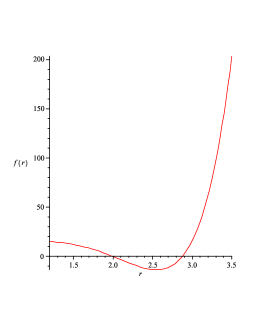
Figure 9: The roots of $f(r)$ for M=2,G=1,$\beta=1$,$Q=\sqrt{2},l^{2}=80$.

References

[1] N. Dadhich, R. Maartens, P. Papadopolous and V. Rezania, Phys. Lett. B487, 1(2000).
[2] A. Chamblin, H.S. Reall, H.A. Shinkai and T. Shiromizu, Phys.Rev.D63, 064015(2001).
[3] T. Shiromizu, K. Maeda and M. Sasaki, Phys.Rev.D62, 024012(2000).
[4] L. D. Landau, The Classical Theory of Fields, (Pergamon, 1973).
[5] F. Rahaman, Int. J. Mod. Phys. D, 9(5), 627-632
(2000) ; F. Rahaman et al, Czech.J.Phys.53,115(2003).
[6] S. Chakraborty, Gen. Rel. Grav. 28, 1115(1996);
S. Chakraborty, F. Rahaman, Pramana 51, 689(1998).
[7] D. R. Brill, P. L. Chrzanowski, C. M. Pereira, E. D. Fackerell, and J. R. Ipser, Phys. Rev. D, 5, 1913 (1972).
[8] S. Chandrasekhar, The Mathematical Theory of Black Holes.
[9] Bryce. s. DeWitt, Quantum Field Theory in Curved Spacetime, Phys. Rep., 19(6),p.295-357, Aug 1975.
[10] Ya. B. Zel dovich, Soviet Phys. JEPT, 35, 1085 1087, (1972).
[11] A. A. Starobinskii, Soviet Phys. JEPT, 37, 28 32, (1973).
[12] R. M. Wald, General Relativity, (Overseas India, New Delhi, 2006).
[13] S. Basak, P. Majumdar, Class.Quant.Grav. 20, 2929-2936 (2003).
[14] S. Basak, P. Majumdar, Class.Quant.Grav. 20, 3907-3914 (2003).
[15] C. Misner, Phys.Rev.Lett.28, 994 (1972)
[16] K Shiraishi, Mod.Phys.Lett.A, 37, 3449 (1992); M H
Ali, Gen.Rel.Grav., 37, 977 (2007).