Ergodic Properties of Fractional Brownian-Langevin Motion

Abstract

We investigate the time average mean square displacement $\overline{\delta^{2}}(x(t))=\int_{0}^{t-\Delta}[x(t^{\prime}+\Delta)-x(t^{\prime})]^{2}dt^{\prime}/(t-\Delta)$ for fractional Brownian and Langevin motion. Unlike the previously investigated continuous time random walk model $\overline{\delta^{2}}$ converges to the ensemble average $\langle x^{2}\rangle\sim t^{2H}$ in the long measurement time limit. The convergence to ergodic behavior is however slow, and surprisingly the Hurst exponent $H=3/4$ marks the critical point of the speed of convergence. When $H<3/4$, the ergodicity breaking parameter $\mbox{EB}=\mbox{Var}(\overline{\delta^{2}})/\langle\overline{\delta^{2}}\rangle^{2}\sim k(H)\cdot\Delta\cdot t^{-1}$, when $H=3/4$, $\mbox{EB}\sim(9/16)(\ln t)\cdot\Delta\cdot t^{-1}$, and when $3/4<H<1,\mbox{EB}\sim k(H)\Delta^{4-4H}t^{4H-4}$. In the ballistic limit $H\to 1$ ergodicity is broken and $\mbox{EB}\sim 2$. The critical point $H=3/4$ is marked by the divergence of the coefficient $k(H)$. Fractional Brownian motion as a model for recent experiments of sub-diffusion of mRNA in the cell is briefly discussed and comparison with the continuous time random walk model is made.

I Introduction

Fractional calculus, e.g. $d^{1/2}/dt^{1/2}$, is a powerful mathematical tool for the investigation of physical and biological phenomena with long-range correlations or long memory Metzler:00 . For example fractional calculus describes the mechanical memory of viscoelastic materials Mainardi:88 . An important application of fractional calculus is in the stochastic modeling of anomalous diffusion. Fractional Fokker-Planck equations describe the long time behavior of the continuous time random walk (CTRW) model, when waiting times and/or jump lengths have power-law distributions Barkai:00 ; Barkai:01 ; Metzler:00 ; Deng:07 . A different stochastic approach to anomalous diffusion is based on fractional Brownian motion (fBM) Mandelbrot:68 which is related to recently investigated fractional Langevin equations (see details below) Goychuk:07 ; Min:05 ; Burov:08 .

Recent single particle tracking of mRNA molecules Golding:06 and lipid granules Tolic:04 in living cells revealed that time averaged mean square displacement $\overline{\delta^{2}}$ (defined below more precisely) of individual particles remains a random variable while indicating that the particle motion is sub-diffusive. This means that the time averages are not identical to ensemble averages. Such breaking of ergodicity was investigated within the sub-diffusive CTRW model He:08 ; Klafter:08 . It was shown that transport and diffusion constants extracted from single particle trajectories remain random variables, even in the long measurement time limit. For a non-technical point of view on this problem see Sokolov:08 . Here we consider three stochastic models of anomalous diffusion: fBM and the under-damped and the over-damped fractional Langevin equation. Except for limiting cases (i.e. ballistic diffusion) we find that the time average $\overline{\delta^{2}}$, in the long measurement time limit, is identical to the ensemble average $\langle x^{2}\rangle$, indicating that these models are ergodic. Note however, that experiments on anomalous dynamics of particles in the cell are always conducted for finite times (due to the life time of the cell). Here we find the finite time corrections to ergodic behavior, namely we give estimates on how far will a finite time measurement of anomalous diffusion deviate from the ensemble average. Since the convergence to ergodic behavior is slow our results seem particularly important to finite time experiments. The problem of estimating diffusion constants from single particle tracking, for normal diffusion, is already well investigated Saxton:97 .

In recent years there was much interest in non-ergodicity of anomalous diffusion processes. A well investigated system are blinking quantum dots Dahan:03 ; Margolin:05 , which exhibit a Lévy walk type of dynamics (a super-diffusive process). Very general formula for the distribution of time averages for weakly non ergodic systems was derived in Rebenshtok:07 , and this framework was shown to describe the sub-diffusive CTRW Bel:05 . Bao et al have investigated ergodicity breaking for stochastic dynamics described by the generalized Langevin equation Bao:05 . They considered the time averaged velocity variance. The latter converges to $k_{B}T/m$ in thermal equilibrium if the process is ergodic. It was shown Bao:05 that under certain conditions the generalized Langevin equation is non ergodic (see also Lee:01 ; Oliv:03 ; Costa:06 ; Dhar:07 ; Plyukhin:08 ). Our work, following the recent experiments Tolic:04 ; Golding:06 , considers the time average of the mean square displacements which yields information on diffusion constants. In contrast with Bao:05 , we consider an out of equilibrium situation, because our observable: the coordinate of the particle does not reach an equilibrium, since the system is infinite.

II Stochastic Models

II.1 Fractional Brownian Motion

Fractional Brownian motion is generated from fractional Gaussian noise, like Brownian motion from white noise. Mandelbrot and van Ness Mandelbrot:68 defined fBM with

$$\begin{array}[]{c}\displaystyle B_{H}(t):=\frac{1}{\Gamma(H+\frac{1}{2})}\left(\int_{0}^{t}(t-\tau)^{H-\frac{1}{2}}dB(\tau)\right.\\ \displaystyle\left.+\int_{-\infty}^{0}[(t-\tau)^{H-\frac{1}{2}}-(-\tau)^{H-\frac{1}{2}}]dB(\tau)\right),\end{array}$$ (1)

where $\Gamma$ represents the Gamma function and $0<H<1$ is called the Hurst parameter. The integrator $B$ is ordinary Brownian motion. Note that $B$ is recovered when taking $H=1/2$. The right hand side of Eq. (1) is the sum of two independent Gaussian processes. In the definition, for the first Gaussian process, we identify the so-called fBM of Riemann-Liouville type Lim:02 . Standard fBM, i.e. Eq. (1), is the only Gaussian self-similar process with stationary increments Mandelbrot:68 . The variance of $B_{H}(t)$ is $2D_{H}t^{2H}$, where $D_{H}=(\Gamma(1-2H)\cos(H\pi))/(2H\pi)$. In the following, for some given $H$, we denote the trajectory sample of fBM $x(t)$. The properties that uniquely characterize the fBM can be summarized as follows: $x(t)$ has stationary increments; $x(0)=0$ and $\langle x(t)\rangle=0$ for $t\geq 0$; $\langle x^{2}(t)\rangle=2D_{H}t^{2H}$ for $t\geq 0$; $x(t)$ has a Gaussian distribution for $t>0$. From the above properties, the covariance function is Samorodnitsky:94 ,

$$\langle x(t_{1})x(t_{2})\rangle=D_{H}(t_{1}^{2H}+t_{2}^{2H}-|t_{1}-t_{2}|^{2H}),~{}~{}t_{1},t_{2}>0.$$ (2)

The non-independent increment process of fBM, called fractional Gaussian noise (fGn), is given by

$$\xi(t)=\frac{dx(t)}{dt},~{}~{}t>0,$$ (3)

which is a stationary Gaussian process and has a standard normal distribution for any $t>0$. The mean $\langle\xi(t)\rangle=0$ and the covariance is

$$\langle\xi(t_{1})\xi(t_{2})\rangle=2D_{H}H(2H-1)|t_{1}-t_{2}|^{2H-2},~{}~{}t_{1},t_{2}>0.$$ (4)

II.2 Fractional Langevin Equation

The standard Langevin equation with white noise can be extended to a generalized Langevin equation with a power-law memory kernel. Such an approach was recently used to model dynamics of single proteins by the group of Xie Min:05 and can be derived from the Kac-Zwanzig model of Brownian motion Kupferman:04 . The under-damped fractional Langevin equation reads

$$m\frac{d^{2}y(t)}{dt^{2}}=-\bar{\gamma}\int_{0}^{t}(t-\tau)^{2H-2}\frac{dy}{d\tau}d\tau+\eta\cdot\xi(t),$$ (5)

where according to the fluctuation dissipation theorem

$$\eta=\sqrt{\frac{k_{B}T\bar{\gamma}}{2D_{H}H(2H-1)}},$$

$\xi(t)$ is fGn defined in Eqs. (3) and (4), $1/2<H<1$ is the Hurst parameter, $\bar{\gamma}>0$ is a generalized friction constant. Eq. (5) is called a fractional Langevin equation since the memory kernel yields a fractional derivative of the velocity (hint use Laplace transform or see Metzler:00 ; Li:07 ). Note that if $0<H<1/2$ the integral over the memory kernel diverges, and hence it is assumed that $1/2<H<1$. This leads to sub-diffusive behavior $\langle y^{2}\rangle\sim t^{2-2H}$. An over-damped fractional Langevin equation, where Newton’s acceleration term is neglected reads Min:05

$$0=-\bar{\gamma}\int_{0}^{t}(t-\tau)^{2H-2}\frac{dz}{d\tau}d\tau+\eta\cdot\xi(t).$$ (6)

In what follows we investigate ergodic properties of the processes $x(t),y(t)$ and $z(t)$.

III Ergodic Properties

We consider the time average

$$\overline{\delta^{2}}(x(t))=\frac{\int_{0}^{t-\Delta}[x(t^{\prime}+\Delta)-x(t^{\prime})]^{2}dt^{\prime}}{t-\Delta},$$ (7)

which is a random variable depending on the stochastic path $x(t)$. Here $\Delta$ is called the lag time. As is well-known, for normal Brownian motion, the ensemble average mean square displacement is $\langle x^{2}(t)\rangle=2D_{1}t$ while the time average mean square displacement of the single trajectory $\overline{\delta^{2}}(x(t))=2D_{1}\Delta$ in statistical sense and in the long measurement time limit. Hence we may use in experiment a single trajectory of a Brownian particle to estimate the diffusion constant $D_{1}$. Will similar ergodic behavior be found also for fBM?

III.1 Fractional Brownian Motion

If the average of the random variable $\overline{\delta^{2}}$ is equal to the ensemble average $\langle x^{2}\rangle$, and if the variance of $\overline{\delta^{2}}$ tends to zero when the measurement time is long the process is ergodic, since then the distribution of $\overline{\delta^{2}}$ tends to a delta function centered on the ensemble average. For fBM, using Eqs. (2) and (7)

$$\langle\overline{\delta^{2}}(x(t))\rangle=\frac{\int_{0}^{t-\Delta}\langle[x(t^{\prime}+\Delta)-x(t^{\prime})]^{2}\rangle\textrm{d}t^{\prime}}{t-\Delta}=2D_{H}\Delta^{2H},$$ (8)

hence $\langle\overline{\delta^{2}}\rangle=\langle x^{2}\rangle$ for all times. The variance of $\overline{\delta^{2}}(x(t))$ is,

$${\rm Var}(\overline{\delta^{2}}(x(t)))=\left\langle\left(\overline{\delta^{2}}(x(t))\right)^{2}\right\rangle-\left\langle\overline{\delta^{2}}(x(t))\right\rangle^{2}.$$ (9)

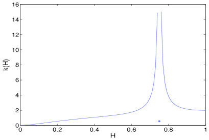
Figure 1: The function of $k(H)$ Eq. (12).

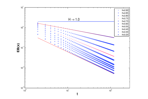
Figure 2: The EB parameter Eq. (11) for fractional Brownian motion $x(t)$ versus time $t$, for different values of Hurst exponent. Here we present exact results obtained directly by calculating Eqs. (8,16,16). The two solid lines (red on line) are the asymptotic theory Eq. (11) for $H=0.2$ and $H=0.9$. In the ballistic limit $H\to 1$ we get non-ergodic behavior. Notice that for $H<3/4$, and long $t$ the curves are parallel to each other due to the ${\rm EB}\sim t^{-1}$ law valid for $H<3/4$, while for $H>3/4$ the slopes are changing as we vary $H$. The lag time is $\Delta=1$.

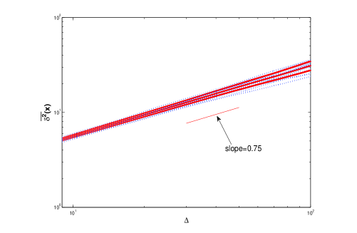
Figure 3: We simulate fBM and present the time average $\overline{\delta^{2}}(x(t))$ versus $\Delta$ (dotted curves blue on line). We show $23$ trajectories, the solid line in the middle being the average of the trajectories. We observe $\overline{\delta^{2}}(x(t))\propto\Delta^{3/4}$, similar to that in Tolic:04 ; Golding:06 . The measurement time is $t=10^{4},~{}H=3/8,~{}D_{H}=1/2$. Line with a slope of $0.75$ is drawn to guide the eye. We also show $\langle\overline{\delta}^{2}\rangle\pm\sqrt{\mbox{Var}(\overline{\delta^{2}})}$ (two solid lines red on line) obtained from Eqs. (8, 23) which give an analytical estimate on the scatter of the data.

A dimensionless measure of ergodicity breaking (EB) is the parameter,

$${\rm EB}(x(t))=\frac{{\rm Var}(\overline{\delta^{2}}(x(t)))}{\left\langle\overline{\delta^{2}}(x(t))\right\rangle^{2}},$$ (10)

which is zero in the limit $t\to\infty$ if the process is ergodic. In the next sub-section we derive our main result, valid for large $t$, we find:

$${\rm EB}(x(t))\thicksim\left\{\begin{array}[]{ll}k(H)\frac{\Delta}{t},&0<H<\frac{3}{4},\\ \\ k(H)\frac{\Delta}{t}\ln t,&H=\frac{3}{4},\\ \\ k(H)(\frac{\Delta}{t})^{4-4H},&\frac{3}{4}<H<1,\end{array}\right.$$ (11)

where

$$k(H)=\left\{\begin{array}[]{ll}\int_{0}^{\infty}((\tau+1)^{2H}+|\tau-1|^{2H}-2\tau^{2H})^{2}d\tau,&0<H<\frac{3}{4},\\ \\ 4H^{2}(2H-1)^{2}=\frac{9}{16},&H=\frac{3}{4},\\ \\ (\frac{4}{4H-3}-\frac{4}{4H-2})H^{2}(2H-1)^{2},&\frac{3}{4}<H<1.\end{array}\right.$$ (12)

The most remarkable result is that $k(H)$ diverges when $H\to 3/4$, $H=3/4$ marks a non smooth transition in the properties of fractional Brownian motion, see Fig. 1. Notice that $k(H)\to 0$ when $H\to 0$ so the asymptotic convergence is expected to hold only after very long times when $H$ is small, since then the diffusion process is very slow. When $H\to 1$ we have ${\rm EB}(x(t))\sim 2$ indicating ergodicity breaking, see Fig. 2.

Fig. 3 displays the simulations of $\overline{\delta^{2}}(x(t))$ showing the randomness of the time average for finite time measurements. In this simulation we generate single trajectories using the Hosking method Hosking:84 , and then perform the time average to find $\overline{\delta^{2}}$. The Fig. mimics the experimental results on single lipid granule in a yeast cell and of mRNA molecules inside a living E-coli cells Tolic:04 ; Golding:06 , where $H=3/8$ was recorded. Note however that the scatter of the experiments data seems larger (see Figs. in Tolic:04 ; Golding:06 ), at least with the naked eye. Further we did not consider in our simulations the effect of the cell boundary. Direct comparison at this stage between experiments and stochastic theory is impossible, since the number of measured trajectories is small.

III.2 Derivation of Main Result Eq.(11)

From Eq. (8),

$$\left\langle\left(\overline{\delta^{2}}(x(t))\right)^{2}\right\rangle=\frac{\int_{0}^{t-\Delta}\textrm{d}t_{1}\int_{0}^{t-\Delta}\textrm{d}t_{2}\langle[x(t_{1}+\Delta)-x(t_{1})]^{2}[x(t_{2}+\Delta)-x(t_{2})]^{2}\rangle}{(t-\Delta)^{2}}.$$ (13)

Using Eq. (2) and the following formula for Gaussian process with mean zero Kubo:95 ,

$$\langle x(t_{1})x(t_{2})x(t_{3})x(t_{4})\rangle=\langle x(t_{1})x(t_{2})\rangle\langle x(t_{3})x(t_{4})\rangle+\langle x(t_{1})x(t_{3})\rangle\langle x(t_{2})x(t_{4})\rangle+\langle x(t_{1})x(t_{4})\rangle\langle x(t_{2})x(t_{3})\rangle,$$

we obtain

$$\langle[x(t_{1}+\Delta)-x(t_{1})]^{2}[x(t_{2}+\Delta)-x(t_{2})]^{2}\rangle=4D_{H}^{2}\Delta^{4H}+2D_{H}^{2}\{|t_{1}+\Delta-t_{2}|^{2H}+|t_{2}+\Delta-t_{1}|^{2H}-2|t_{1}-t_{2}|^{2H}\}^{2}.$$ (14)

From Eqs. (8,9,13,14), we have

$${\rm Var}(\overline{\delta^{2}}(x(t))) = \underbrace{4D_{H}^{2}\left\{\int_{0}^{2\Delta}(t-\Delta-t^{\prime})\{(t^{\prime}+\Delta)^{2H}+|t^{\prime}-\Delta|^{2H}-2{t^{\prime}}^{2H}\}^{2}\textrm{d}t^{\prime}\right\}/(t-\Delta)^{2}}_{V_{1}}$$ (16)

$$+\underbrace{4D_{H}^{2}\left\{\int_{2\Delta}^{t-\Delta}(t-\Delta-t^{\prime})\{(t^{\prime}+\Delta)^{2H}+(t^{\prime}-\Delta)^{2H}-2{t^{\prime}}^{2H}\}^{2}\textrm{d}t^{\prime}\right\}/(t-\Delta)^{2}}_{V_{2}}.$$

When $t>>\Delta$ we may approximate the upper limit in the integral of $V_{2}$ with $t$, and $1/(t-\Delta)^{2}\to 1/t$. We then make a change of variables according to $x=(t-t^{\prime})/t$ and find

$$V_{2}=4D_{H}^{2}t^{4H}\int_{0}^{1}x(1-x)^{4H}\left[\left(1+{\Delta\over t(1-x)}\right)^{2H}+\left|1-{\Delta\over t(1-x)}\right|^{2H}-2\right]^{2}{\rm d}x.$$ (17)

We expand in $\Delta/t$ to second order and find

$$V_{2}\sim 4D_{H}^{2}t^{4H}\left({\Delta\over t}\right)^{4}H^{2}\left(2H-1\right)^{2}\int_{0}^{1}x(1-x)^{4H-4}{\rm d}x.$$ (18)

The integral is finite only if $H>3/4$ hence for $H\leqslant 3/4$ we will soon use a different approach. We see that $V_{2}\sim t^{4H-4}$ while it is easy to show that $V_{1}\sim 1/t$ hence for $H>3/4$ we find after solving the integral

$${\rm Var}(\overline{\delta^{2}}(x(t)))\sim 16D_{H}^{2}t^{4H}\left({\Delta\over t}\right)^{4}H^{2}(2H-1)^{2}\left({1\over 4H-3}-{1\over 4H-2}\right).$$ (19)

Now we write the variance as

$${\rm Var}(\overline{\delta^{2}}(x(t)))={4D_{H}^{2}\over(t-\Delta)^{2}}\int_{0}^{t-\Delta}\left(t-\Delta-t^{\prime}\right)\left[\left(t^{\prime}+\Delta\right)^{2H}+|t^{\prime}-\Delta|^{2H}-2{t^{\prime}}^{2H}\right]^{2}{\rm d}t^{\prime}.$$ (20)

Changing variables according to $\tau=t^{\prime}/\Delta$ we find

$${\rm Var}(\overline{\delta^{2}}(x(t)))={4D_{H}^{2}\over(t-\Delta)}\Delta^{4H+1}\int_{0}^{t/\Delta-1}{\rm d}\tau\left[\left(1+\tau\right)^{2H}+|1-\tau|^{2H}-2\tau^{2H}\right]^{2}+{\rm Corr}.$$ (21)

The correction term is

$$\mbox{Corr}=-{4D_{H}^{2}\over(t-\Delta)^{2}}\Delta^{4H+2}\int_{0}^{t/\Delta-1}{\rm d}\tau\left[\left(1+\tau\right)^{2H}+|1-\tau|^{2H}-2\tau^{2H}\right]^{2}\tau.$$ (22)

Taking the upper limit of the integral in Eq. (21) to $\infty$ we find that for $H<3/4$ and long times

$${\rm Var}(\overline{\delta^{2}}(x(t)))\sim 4D_{H}^{2}\Delta^{4H}\left({\Delta\over t}\right)\int_{0}^{\infty}{\rm d}\tau\left[\left(1+\tau\right)^{2H}+|1-\tau|^{2H}-2\tau^{2H}\right]^{2}.$$ (23)

This is because ${\rm Corr}\sim t^{\max\{4H-4,-2\}}$ (we prove this in the following) and this term is smaller than the leading term which has a $1/t$ decay, since $H<3/4$.

Now we estimate the correction term Eq. (22)

$$\frac{1}{t^{2}}\int_{0}^{t/\Delta-1}{\rm d}\tau\left[\left(1+\tau\right)^{2H}+|1-\tau|^{2H}-2\tau^{2H}\right]^{2}\tau=\frac{1}{t^{2}}\left(\int_{0}^{2}{\rm d}\tau+\int_{2}^{t/\Delta-1}{\rm d}\tau\right)\left[\left(1+\tau\right)^{2H}+|1-\tau|^{2H}-2\tau^{2H}\right]^{2}\tau.$$ (24)

Using the Lagrange reminder of Taylor expansion in $1/\tau$, when $H\leqslant\frac{3}{4}$ we have

$$\begin{array}[]{l}\displaystyle\frac{1}{t^{2}}\int_{2}^{t/\Delta-1}{\rm d}\tau\left[\left(1+\tau\right)^{2H}+|1-\tau|^{2H}-2\tau^{2H}\right]^{2}\tau\\ \\ \displaystyle=\frac{1}{t^{2}}\int_{2}^{t/\Delta-1}{\rm d}\tau\left[\left(1+\frac{1}{\tau}\right)^{2H}+\left|1-\frac{1}{\tau}\right|^{2H}-2\right]^{2}\tau^{4H+1}\\ \\ \displaystyle=\frac{1}{t^{2}}\int_{2}^{t/\Delta-1}{\rm d}\tau\left[(1+\xi)^{2H-2}+(1-\xi)^{2H-2}\right]2H(2H-1)\tau^{4H-3},~{}~{}~{}~{}\xi\in[0,\frac{1}{2}]\\ \\ \displaystyle\sim t^{\max\{4H-4,-2\}}.\end{array}$$ (25)

For $H=\frac{3}{4}$ we use Eq. (21), however now we expand to third order and find

$${\rm Var}(\overline{\delta^{2}}(x(t)))\sim 16D_{H}^{2}H^{2}(2H-1)^{2}\Delta^{3}\ln t\left(\frac{\Delta}{t}\right),$$ (26)

while the correction term ${\rm Corr}\sim t^{-1}$ [see Eq. (25)] is negligible. Using Eqs. (19,23,26) we derive Eq. (11).

III.3 Over Damped Fractional Langevin Equation

We now analyze the over-damped fractional Langevin Eq. (6), we can rewrite it in a convenient way as

$$\bar{\gamma}\Gamma(2H-1)D^{1-2H}Dz(t)=\eta\cdot\xi(t),$$ (27)

where $D=d/dt$, and $D^{1-2H}$ is the Riemann-Liouville fractional integral of $2H-1$ order. Using the tools of fractional calculus Li:07 , we get

$$\bar{\gamma}\Gamma(2H-1)z(t)=\eta\cdot D^{2H-2}\xi(t).$$ (28)

Then since $\langle\xi(t)\rangle=0$ we have $\langle z(t)\rangle=0$, and

$$\langle z(t_{1})z(t_{2})\rangle=D_{F}(t_{1}^{2-2H}+t_{2}^{2-2H}-|t_{1}-t_{2}|^{2-2H}),$$ (29)

where

$$D_{F}=\frac{k_{B}T\pi\csc[\pi({2-2H})]}{\bar{\gamma}(2-2H)\Gamma^{2}(2H-1)\Gamma^{2}(2-2H)}.$$

From Eq. (29) we learn that Eq. (27) exhibits the same behavior as fBM Eq. (1) in the sub-diffusion case. Note that for fBM $\langle x^{2}\rangle\sim t^{\alpha}$ with $\alpha=2H$ while for the fractional Langevin equation $\langle z^{2}\rangle\sim t^{\alpha}$ with $\alpha=2-2H$, and of course

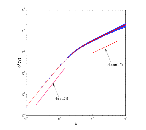
Figure 4: The time average $\overline{\delta^{2}}(y(t))$ is a random variable depending on the underlying trajectory. Total 23 trajectories, besides the solid line with mark $\circ$ being the average of the 23 trajectories, are plotted. The measurement time is $t=10^{4},2-2H=0.75,~{}D_{H}=1/2,~{}k_{B}=1,~{}m=1,~{}\bar{\gamma}=1,~{}v_{0}=1,~{}T=1$. Lines with slopes of $2.0$ (ballistic motion in short times) and $0.75$ (sub-diffusion for long times) are drawn to guide the eye. For long $\Delta$ the behavior of the under-damped motion is similar to usual fractional Brownian motion.

the diffusion constants have different dependencies on parameters of the noise. However these minor modifications do not change our main result for $0<H<1/2$ obtained in the previous section (only switch the value $2H$ to $2-2H$). See this note that the EB parameter depends on the behavior of correlation function Eq. (2) and the latter are identical for the processes $x(t)$ and $z(t)$ in the sub-diffusion case, so ${\rm EB}(z)\sim{\rm EB}(x)$.

III.4 Under Damped Fractional Langevin Equation

We now analyze the fractional Langevin equation with power-law kernel, namely, Eq. (5),

$$m\frac{d^{2}y(t)}{dt^{2}}=-\bar{\gamma}\int_{0}^{t}(t-\tau)^{2H-2}\frac{dy}{d\tau}d\tau+\eta\cdot\xi(t),$$ (30)

with $dy(0)/dt=v_{0}$, $y(0)=0$, where $v_{0}$ is the initial velocity. The solution of the stochastic Eq. (30) is

$$\begin{array}[]{lll}y(t)&=&v_{0}\cdot t\cdot E_{2H,2}(-\gamma\cdot t^{2H})\\ &&+\frac{\eta}{m}\int_{0}^{t}(t-\tau)\cdot E_{2H,2}(-\gamma\cdot(t-\tau)^{2H})\xi(\tau)d\tau,\end{array}$$

where $\gamma=(\bar{\gamma}\Gamma(2H-1))/m$ and the generalized Mittag-Leffler function is

$$E_{\alpha,\beta}(t)=\sum\limits_{n=1}^{\infty}\frac{t^{n}}{\Gamma(\alpha n+\beta)},$$

and $E_{\alpha,\beta}(-t)\thicksim(t\Gamma(\beta-\alpha))^{-1}$ when $t\rightarrow+\infty$.

We have

$$\langle y(t)\rangle=v_{0}\cdot t\cdot E_{2H,2}(-\gamma\cdot t^{2H})\thicksim\frac{v_{0}}{\gamma}\frac{t^{1-2H}}{\Gamma(2-2H)},$$ (31)

and

$$\begin{array}[]{lll}\langle y^{2}(t)\rangle&=&\frac{2k_{B}T}{m}t^{2}E_{2H,3}(-\gamma\cdot t^{2H})\\ \\ &\thicksim&\frac{2k_{B}T}{\bar{\gamma}\Gamma(2H-1)\Gamma(3-2H)}\cdot t^{2-2H},\end{array}$$ (32)

where the thermal initial condition: $v_{0}^{2}=k_{B}T/m$ is assumed.

Note that for short times we have $\langle y^{2}(t)\rangle\sim(k_{B}T/m)t^{2}$. Eqs. (31) and (32) were found Lutz:01 ; BarkaiSilbey:00 .

The covariance function of $y(t)$ reads

$$\begin{array}[]{lll}\langle y(t_{1})y(t_{2})\rangle&=&v_{0}^{2}t_{1}t_{2}E_{2H,2}(-\gamma t_{1}^{2H})E_{2H,2}(-\gamma t_{2}^{2H})\\ \\ &&\displaystyle+\frac{k_{B}T\bar{\gamma}}{m^{2}}\int_{0}^{t_{2}}\int_{0}^{t_{1}}d\tau ds\cdot(t_{1}-\tau)E_{2H,2}(-\gamma(t_{1}-\tau)^{2H})(t_{2}-s)E_{2H,2}(-\gamma(t_{2}-s)^{2H})|\tau-s|^{2H-2}.\end{array}$$ (33)

When $t_{1},\,t_{2}$ tend to infinity,

$$\langle y(t_{1})y(t_{2})\rangle\thicksim\frac{k_{B}T}{\bar{\gamma}\Gamma^{2}(2H-1)\Gamma^{2}(2-2H)}\int_{0}^{t_{2}}\int_{0}^{t_{1}}d\tau ds\cdot(t_{1}-\tau)^{1-2H}(t_{2}-s)^{1-2H}|\tau-s|^{2H-2},$$ (34)

i.e., the covariance of $y(t)$ approximates to the ones of $z(t)$, so we can expect in the long-time limit

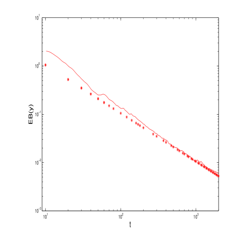
Figure 5: The ergodicity breaking parameter ${\rm EB}(y)$ versus $t$. Simulations of $200$ trajectories were used with $2-2H=0.75,~{}\Delta=10,~{}k_{B}=1,~{}m=1,~{}\bar{\gamma}=1,~{}v_{0}=1,~{}T=1$. The stars $*$ is the theoretical result Eq. (11) with corresponding parameter values (without fitting).

$$\langle\overline{\delta^{2}}(y)\rangle\thicksim\langle\overline{\delta^{2}}(z)\rangle\thicksim\langle\overline{\delta^{2}}(x)\rangle,$$ (35)

and

$${\rm EB}(y)\thicksim{\rm EB}(z)\thicksim{\rm EB}(x).$$ (36)

The simulations Numerical:08 , Fig. 4, confirms Eq. (35) and Figs. 5 and 6, support Eq. (36). Note that for short times we have a ballistic behavior for $y(t)$ (see Fig. 4), but not for $z(t)$ and $x(t)$, so clearly both $\Delta$ and $t$ must be large for Eq. (36) to hold.

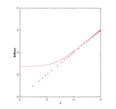
Figure 6: The ergodicity breaking parameter ${\rm EB}(y)$ versus $\Delta$. Total 200 trajectories are used to compute the average and variance, the measurement time $t=10^{4}$, $2-2H=0.75,~{}k_{B}=1,~{}m=1,~{}\bar{\gamma}=1,~{}v_{0}=1,~{}T=1$. The stars $*$ are the theoretical result Eq. (11) with corresponding parameter values. We see that results found from the under-damped Langevin equation converge to our analytical theory based on fBM.

IV Discussion

We showed that the fractional processes $x(t)$, $y(t)$ and $z(t)$ are ergodic. The ergodicity breaking parameter decays as a power-law to zero. In the ballistic limit $\langle x^{2}\rangle\sim t^{2}$ non ergodicity is found. For the opposite localization limit $\langle x^{2}\rangle\sim t^{0}$ (i.e. $H\to 0$ for fBM) the asymptotic convergence is reached only after very long times. Our most surprising result is that the transition between the localization limit and ballistic limit is not smooth. When $H=3/4$ the EB is changed and the amplitude $k(H)$ diverges. Other very different critical exponents of fractional Langevin equations were recently found in Burov:08 . There the critical exponents mark transitions between over-damped and under-damped motion. So stochastic fractional processes possess a zoo of critical exponents. Let us now compare between our results and those derived based on the CTRW model He:08 . The most striking difference is that for the CTRW model we have non ergodic behavior even in the long time limit. It is attempting to conclude that this indicates that the underlying stochastic motion for the mentioned experiments in the cell is of CTRW nature. However, as mentioned in the introduction experiments are conducted for finite times, and hence what may seem as a deviation from ergodic behavior may actually be a finite time effect. Here we gave analytical predictions for the deviations from ergodicity for finite time measurement, based on three fractional models. The EB parameter depends on measurement time and lag time, and can be used to compare experimental data with predictions of fractional equations (the EB parameter for the CTRW is given in He:08 ). It should be noted however that for sub-diffusion in the cell, effects of the boundary of the cell, may be important, and these effects where not considered in this text. Another important difference is that for an infinite system we have for the CTRW $\langle\overline{\delta^{2}}\rangle\sim\Delta/t^{\alpha}$, so the time average procedure yields a linear dependence on $\Delta$ and an aging effect with respect to the measurement time. Hence for CTRW an anomalous diffusion process may seem normal with respect to $\Delta$ He:08 ; Barkai:03a ; Barkai:03b ; Klafter:08 . In contrast for the fractional models we investigated here, we have $\langle\overline{\delta^{2}}\rangle\sim\Delta^{\alpha}$ which is the same as the ensemble average $\langle x^{2}\rangle\sim t^{\alpha}$. The main difference between the two approaches, is that the CTRW process is non-stationary. It would be interesting to investigate fractional Riemann-Liouville Brownian motion (Eq. (1) without the integral from $-\infty$ to $0$) which is a non-stationary process.

Acknowledgement This work was supported by the Israel Science Foundation. EB thanks S. Burov for discussions.

References

- (1) R. Metzler and J. Klafter, Phys. Rep. 339, 1 (2000).
- (2) F. Mainardi and E. Bonetti, Rheologica Acta 26, 64 (1988).
- (3) R. Metzler, E. Barkai, J. Klafter, Phys. Rev. Lett. 82, 3563 (1999).
- (4) E. Barkai, R. Metzler, and J. Klafter, Phys. Rev. E 61, 132 (2000). E. Barkai, ibid 63, 046118 (2001).
- (5) W.H. Deng, J. Comput. Phys. 227, 1510 (2007).
- (6) B.B. Mandelbrot and J.W. van Ness, SIAM Review 10, 422 (1968).
- (7) I. Goychuk and P. Hänggi, Phys. Rev. Lett. 99, 200601 (2007).
- (8) W. Min, G. Luo, B.J. Cherayil, S.C. Kou, and X.S. Xie, Phys. Rev. Lett. 94, 198302, (2005).
- (9) S. Burov and E. Barkai, Phys. Rev. Lett. 100, 070601 (2008).
- (10) I. Golding and E.C. Cox, Phys. Rev. Lett. 96, 098102, (2006).
- (11) I.M. Tolić-Nørrelykke, E.L. Munteanu, G. Thon, L. Oddershede, and K. Berg-Sorensen, Phys. Rev. Lett. 93, 078102 (2004).
- (12) Y. He, S. Burov, R. Metzler, and E. Barkai, Phys. Rev. Lett. 101, 058101 (2008).
- (13) A. Lubelski I. M. Sokolov, and J. Klafter, Phys. Rev. Lett. 100 250602 (2008).
- (14) I.M. Sokolov, Physics 1, 8 (2008).
- (15) J. Saxton, Biophys. J. 72, 1744 (1997).
- (16) X. Brokmann, et al, Phys. Rev. Lett. 90, 120601 (2003).
- (17) G. Margolin and E. Barkai, Phys. Rev. Lett. 94, 080601 (2005).
- (18) A. Rebenshtok and E. Barkai, Phys. Rev. Lett. 99, 210601 (2007).
- (19) G. Bel and E. Barkai, Phys. Rev. Lett. 94, 240602 (2005).
- (20) J.D. Bao, P. Hänggi, and Y.Z. Zhuo, Phys. Rev. E 72, 061107 (2005).
- (21) M.H. Lee, Phys. Rev. Lett. 87, 250601 (2001).
- (22) I.V.L. Costa, R. Morgado, M.V.B.T. Lima, and F.A. Oliveira, Europhys. Lett. 63, 173 (2003).
- (23) I.V.L Costa, et al, Physica A 371, 130 (2006).
- (24) A. Dhar and K. Wagh, Europhys. Lett. 79, 60003 (2007).
- (25) A.V. Plyukhin, Phys. Rev. E. 77, 061136 (2008).
- (26) S.C. Lim and S.V. Muniandy, Phys. Rev. E 66, 021114 (2002).
- (27) G. Samorodnitsky and M. Taqqu, Stable Non-Gaussian Random Processes: Stochastic Models with Infinite Variance (Chapman and Hall, New York, 1994).
- (28) R. Kupferman, J. Stat. Phys. 114, 291 (2004).
- (29) C.P. Li and W.H. Deng, Appl. Math. Comput. 187, 777, (2007).
- (30) W.T. Coffey, Yu.P. Kalmykov, and J.T. Waldron, The Langevin Equation (World Scientific, New Jersey, 2004).
- (31) R. Kubo, M. Toda, and N. Hashitsume, Statistical Physics II: Nonequilibrium statistical mechanics (Springer-Verlag, Heidelberg, 1995).
- (32) E. Lutz, Phys. Rev. E 64, 051106 (2001).
- (33) E. Barkai and R.J. Silbey, J. Phys. Chem. B 104, 3866, (2000).
- (34) J.R.M. Hosking, Water resources research 20, 1898, (1984).
- (35) The detailed numerical scheme and error analysis will be presented in the coming publication.
- (36) E. Barkai and Y.C. Cheng, J. Chem. Phys. 118 6167 (2003),
- (37) E. Barkai, Phys. Rev. Lett. 90 104101 (2003).