On Coxeter diagrams of complex reflection groups

Author : Tathagata Basak

Address : Iowa State University, Department of mathematics, Carver Hall, Ames, IA 50011.

email : tathastu@gmail.com

Abstract: We study Coxeter diagrams of some unitary reflection groups. Using solely the combinatorics of diagrams, we give a new proof of the classification of root lattices defined over $\mathcal{E}=\mathbb{Z}[e^{2\pi i/3}]$: there are only four such lattices, namely, the $\mathcal{E}$–lattices whose real forms are $A_{2}$, $D_{4}$, $E_{6}$ and $E_{8}$. Next, we address the issue of characterizing the diagrams for unitary reflection groups, a question that was raised by Broué, Malle and Rouquier. To this end, we describe an algorithm which, given a unitary reflection group $G$, picks out a set of complex reflections. The algorithm is based on an analogy with Weyl groups. If $G$ is a Weyl group, the algorithm immediately yields a set of simple roots. Experimentally we observe that if $G$ is primitive and $G$ has a set of roots whose $\mathbb{Z}$–span is a discrete subset of the ambient vector space, then the algorithm selects a minimal generating set for $G$. The group $G$ has a presentation on these generators such that if we forget that the generators have finite order then we get a (Coxeter-like) presentation of the corresponding braid group. For some groups, such as $G_{33}$ and $G_{34}$, new diagrams are obtained. For $G_{34}$, our new diagram extends to an “affine diagram” with $\mathbb{Z}/7\mathbb{Z}$ symmetry.

Keywords: Unitary reflection group, Coxeter diagram, Weyl group, simple root.
2000 Mathematics subject classification: 20F55, 20F05, 20F65, 51F25.

1. Introduction

1.1.

Background on unitary reflection groups: Let $G$ be a finite subgroup of the unitary group $U(n)$ generated by complex reflections, such that $G$ acts irreducibly on $\mathbb{C}^{n}$. We shall simply say that $G$ is an unitary reflection group. Let $\mathcal{M}$ be the union of the fixed point sets of the complex reflections in $G$ and let $X_{G}=\mathbb{C}^{n}\setminus\mathcal{M}$. The fundamental group $\operatorname{Braid}(G):=\pi_{1}(X_{G}/G)$ is called the (generalized) braid group associated to $G$. Let $k$ be the minimum number of complex reflections needed to generate $G$. We say that $G$ is well generated if $k=n$. The smallest subfield $F$ of $\mathbb{C}$ that contains all the complex character values of $G$, is called the field of definition of $G$. We say that $G$ is defined over $F$.

Unitary reflection groups were classified by Shephard and Todd in [13]. For a self-contained proof of the classification, which is similar in spirit to part of our work, see [7]. A convenient table of all these groups and their properties may be found in [6]. There is an infinite series, denoted by $G(de,e,r)$, and $34$ others, denoted by $G_{4},G_{5},\dotsb,G_{37}$. Unitary reflection groups have many invariant theoretic properties that are similar to those of the orthogonal reflection groups. Most of these properties were initially established for the unitary reflection groups, via case by case verification through Shephard and Todd’s list. Recently, there has been a lot of progress in trying to find unified and more conceptual proofs. (For example, see [4] and the references therein). However, a coherent theory, like that of the classical Coxeter groups and Weyl groups, is still not in place and many mysteries still remain. One of these mysteries involve the diagrams for unitary reflection groups.

Coxeter presentations of orthogonal reflection groups are encoded in their Coxeter-Dynkin diagrams. Similarly, for each unitary reflection group $G$, there is a diagram $D_{G}$, that encodes a presentation of $G$ (Such a $D_{G}$ is given in [6] for all but six groups. For the remaining six groups presentations of the corresponding braid group were conjectured in [5], in terms of certain diagrams. The proof of this conjecture was completed in [4]). Most of these diagrams were first introduced by Coxeter in [10]. The vertices of $D_{G}$ correspond to complex reflections that form a minimal set of generators for $G$. Other than that, the definition of $D_{G}$ is ad-hoc and case by case. It is curious that even though these diagrams do not have any uniform definition, they contain a lot of non-trivial information about the group $G$. We quote two sample results which state that the weak homotopy type of $X_{G}/G$ and the invariant degrees of $G$ can be recovered from the diagram $D_{G}$.

1.2 Theorem ([4]).

(a) The universal cover of $X_{G}/G$ is contractible.

(b) $G$ has a minimal generating set of complex reflections, $\bar{\mathbf{b}}=\{\bar{b}_{1},\dotsb,\bar{b}_{k}\}$, which can be lifted to a set of generators $\mathbf{b}=\{b_{1},\dotsb,b_{k}\}$ of $\operatorname{Braid}(G)$, with the following property: There is a set of positive homogeneous relations $R^{\prime}_{G}(\mathbf{b})$ in the alphabet $\mathbf{b}$ such that $\operatorname{Braid}(G)$ and $G$ have the following presentations:

$$\operatorname{Braid}(G)\simeq\langle\mathbf{b}|R^{\prime}_{G}(\mathbf{b})\rangle,\text{\; \;}G\simeq\langle\bar{\mathbf{b}}|R^{\prime}_{G}(\bar{\mathbf{b}}),\bar{b}_{i}^{n_{i}}=1\text{\; for all \;}i\rangle,$$

where $n_{i}$ is the order of $\bar{b}_{i}$ in $G$. (These presentations are encoded by a diagram $D_{G}$ with vertex set $\mathbf{b}$, the edges indicating the relations in $R^{\prime}_{G}$).

1.3 Theorem (Th. 5.5 of [12], [5], [4]).

Let $G$ be a well generated unitary reflection group. The Coxeter number of $G$ is defined to be the largest positive integer $h$ such that $e^{2\pi i/h}$ is an eigenvalue of an element of $G$. Then the product of the generators of $G$ corresponding to the vertices of $D_{G}$, in certain order, has eigenvalues $e^{2\pi i(d_{j}-1)/h}$ where $d_{j}$ are the invariant degrees of $G$.

If $G$ is a Weyl group and $V$ is the complexification of the standard representation of $G$, then both 1.2 (due to Briskorn, Saito, Deligne) and 1.3 (probably due to Borel, Chevalley, Steinberg) are classical. These results were first verified for most of the groups in Shephard and Todd’s list by arguments split into many separate cases. Essentially classification free proofs are now known, by recent work of David Bessis (see [4], where the long standing task of showing that $X_{G}$ is $K(\pi,1)$ and finding Coxeter-like presentation for $\operatorname{Braid}(G)$ were completed). But we still do not know of a way to characterize the diagrams for unitary reflection groups.

In this article, we study the diagrams of a few unitary reflection groups. The main results are discussed below. They are motivated by analogies with Weyl groups.

1.4.

Summary of results: Our approach is to view unitary reflection groups as sets of automorphisms of “complex lattices”. Let $\mathcal{E}=\mathbb{Z}[e^{2\pi i/3}]$. The main examples of unitary reflection groups, that we want to study, act as automorphisms of a sequence of $\mathcal{E}$–lattices, namely, $A_{2}^{\mathcal{E}}\subseteq D_{4}^{\mathcal{E}}\subseteq E_{6}^{\mathcal{E}}\subseteq E_{8}^{\mathcal{E}}$. Our interest in these lattices stems from their importance in studying the complex hyperbolic reflection group with $Y_{555}$ diagram and its conjectured connection with the bimonster (see [1], [3]). In section 2, we present a new proof of theorem 2.2 of [1], which states that $A_{2}^{\mathcal{E}},D_{4}^{\mathcal{E}},E_{6}^{\mathcal{E}},E_{8}^{\mathcal{E}}$ are the only “$\mathcal{E}$–root lattices”. Our proof is like the $A$–$D$–$E$ classification of Euclidean root lattices and is similar in spirit to the arguments in [7] and [11]. It is purely a linear algebra argument that only uses the diagrams for the complex reflection groups. This proof should be viewed as an illustration of the usefulness of the “complex diagrams”.

In Section 3 we address the following question, that was raised in [6]: How to characterize the diagrams for the unitary reflection groups? To this end, we describe an algorithm (in 3.8 and 3.9) which, given the group $G$, the integer $k$ and a random vector in $V$, selects a set $\bar{\mathbf{a}}=\{\bar{a}_{1},\dotsb,\bar{a}_{k}\}$ of reflections in $G$. Our algorithm is based on a generalization of a “Weyl vector”. We show that “Weyl vectors” exist for all unitary reflection groups (see theorem 3.5). If $G$ is a Weyl group, then one can easily check that $\bar{\mathbf{a}}$ is a set of simple roots of $G$.

If $G$ is primitive and defined over an imaginary quadratic extension of $\mathbb{Q}$, then we experimentally observe that $\bar{\mathbf{a}}$ is a minimal set of generators of $G$. There exists a set of positive homogeneous relations $R_{G}(\mathbf{a})$ in the alphabet $\mathbf{a}=\{a_{1},\dotsb,a_{k}\}$ such that:

In every execution of the algorithm, the generators $\bar{\mathbf{a}}$ satisfy the relations $R_{G}(\bar{\mathbf{a}})$.

We find that the reflections $\bar{\mathbf{a}}$ form Coxeter’s diagram in the examples of our main interest, namely, the reflection groups related to the $\mathcal{E}$–root lattices. For some groups $G$, namely, $G_{12}$, $G_{29}$, $G_{31}$, $G_{33}$ and $G_{34}$, new diagrams are obtained. More precisely, the generators $\bar{\mathbf{a}}$ selected by the algorithm 3.9 do not satisfy the relations $R^{\prime}_{G}$ known from [6], [5]. In section 4, we verify that:

The group $\operatorname{Braid}(G)$ has a presentation given by $\langle\mathbf{a}|R_{G}(\mathbf{a})\rangle$ and $G$ has a presentation given by $\langle\bar{\mathbf{a}}|R_{G}(\bar{\mathbf{a}}),\bar{a}_{i}^{n_{i}}=1\text{\; for all \;}i\rangle$, that is, Theorem 1.2(b) holds for the new diagrams (see 4.6).

We have verified that Theorem 1.3 also holds for the new diagrams for $G_{29}$, $G_{33}$ and $G_{34}$. The other two groups $G_{12}$ and $G_{31}$ are not well-generated.

Let $G\in\{G_{29},G_{31},G_{33},G_{34}\}$. For these groups, the relations $R_{G}$ that our generators satisfy are different from those previously known. We note that all the relations in $R_{G}$ (i.e. those needed to present $\operatorname{Braid}(G)$) are of the form $x_{0}x_{1}\dotsb x_{m-1}=x_{1}x_{2}\dotsb x_{m}$, for a set of generators $\{x_{i}\colon i\in\mathbb{Z}/k\mathbb{Z}\}$, which form a minimal cycle in the diagram. When $k=2$, these are the Coxeter relations. For most $G$, the group $\operatorname{Braid}(G)$ has a presentation consisting of only this kind of relations (see the table in [6]). Following Conway [8], we call these deflation relations. The deflation relations encountered in $G_{33}$ and $G_{34}$ are, moreover, all “cyclic” (see 4.3, 4.4). For $G_{29}$, $G_{33}$ or $G_{34}$, a presentation of the corresponding braid group is obtained by taking one braid relation for each edge and one deflation relation for each minimal cycle in the diagram. This makes us wonder if the right notion of a diagram for these groups is the $2$ dimensional polyhedral complex obtained by attaching $2$-cells to the minimal cycles in the graphs $D_{G}$, so that, finiteness of $G$ translates into the vanishing of the first homology of the polyhedral complex.

Note that $G_{33}$ and $G_{34}$, are part of a few exceptional cases, in which, the diagrams known in the literature do not have some of the desirable properties. (For example, see question 2.28 in [6] and the remark following it). So there seems to be some doubt whether the diagrams known in the literature for these examples, are the “right ones”.

In section 5 we describe affine diagrams for unitary reflection groups defined over $\mathcal{E}$. The affine diagrams are obtained from the unitary diagrams by adding an extra node. They encode presentations for the corresponding affine complex reflection groups. For each affine diagram, we describe a “balanced numbering” on its vertices, like the $\begin{smallmatrix}&&3&&&&&\\ 2&4&6&5&4&3&2&1\end{smallmatrix}$ numbering on the affine $E_{8}$ diagram. The existence of a balanced numbering on a diagram implies that the corresponding reflection group is not finite. So an affine diagram cannot occur as a full sub-graph of a diagram for a unitary reflection group. These facts, coupled with a combinatorial argument, complete the classification of $\mathcal{E}$–root lattices. The affine diagrams are often more symmetric compared to the unitary diagrams, like in the real case. For example, for $G_{34}$, (which is the reflection group of the Coxeter-Todd lattice $K_{12}^{\mathcal{E}}$), we get an affine diagram with rotational $\mathbb{Z}/7\mathbb{Z}$ symmetry.

The complex root systems that we use in computer experiments are described in the appendix A. Appendix B contains details of proofs of statements made in section 4.

1.5.

Shortcomings of algorithm 3.9: If $G$ is imprimitive or not defined over $\mathbb{Q}$ or an imaginary quadratic extension of $\mathbb{Q}$, then our algorithm does not work, in the sense that the set $\bar{\mathbf{a}}$ of reflections chosen by the algorithm usually do not form a minimal set of generators of $G$. Also, one knows from [6] and [5] that the braid groups of $G_{12}$ and $G_{24}$ can be presented using cyclic deflation relations, but we were unable to find such presentations of these braid groups on the generators selected by our algorithm. So while the algorithm 3.9 does not provide a definite characterization of the diagrams for the unitary reflection groups, the observations in the previous paragraphs seem to indicate that the diagrams have a geometric origin.

We finish this section by introducing some basic definitions and notations to be used.

1.6.

Reflection groups and root systems: Let $V$ be a complex vector space with an hermitian form (always assumed to be linear in the second variable). If $x\in V$, then $\lvert x\rvert^{2}=\langle x,x\rangle$ is called the norm of $x$. Given a vector $x$ of non-zero norm and a root of unity $u\neq 1$, let

$$\phi_{x}^{u}(y)=y-(1-u)\langle x,y\rangle\lvert x\rvert^{-2}x.$$

The automorphism $\phi_{x}^{u}$ of the hermitian vector space $V$ is called an $u$–reflection in $x$, or simply, a complex reflection. The hyperplane $x^{\bot}$ (or its image in the projective space $\mathbb{P}(V)$), fixed by $\phi_{x}^{u}$, is called the mirror of reflection. A complex reflection group $G$ is a discrete subgroup of $\operatorname{Aut}(V,\langle\;,\>\rangle)$, generated by complex reflections. A mirror of $G$ is a hyperplane fixed by a reflection in $G$. A complex reflection (resp. complex reflection group) is called a unitary reflection (resp. unitary reflection group) if the hermitian form on $V$ is positive definite. We shall omit the words “complex” or “unitary”, if they are clear from context. A unitary reflection group $G$ acting on $V$ is reducible (resp. imprimitive) if $V$ is a direct sum $V=V_{1}\oplus\dotsb\oplus V_{l}$ such that $0\neq V_{1}\neq V$ and each $V_{j}$ is fixed by $G$ (resp. the collection of $V_{j}$ is stabilized by $G$). Otherwise $G$ is irreducible (resp. primitive). Unless otherwise stated, we always assume that $G$ is irreducible.

Let $G$ be a unitary reflection group acting on $\mathbb{C}^{k}$ with the standard hermitian form. Let $F$ be the field of definition of $G$. Let $\mathcal{O}$ be the ring of integers in $F$. Let $\mathcal{O}^{*}$ be the group of units of $\mathcal{O}$. A vector $r$ in an $\mathcal{O}$–module $K$ is primitive if $r=mr^{\prime}$ with $m\in\mathcal{O}$ and $r^{\prime}\in K$ implies that $m\in\mathcal{O}^{*}$. Let $\Phi$ be a set of primitive vectors in $\mathcal{O}^{k}$ such that:

• $\Phi$ is stable under the action of $G$,

• $\{r^{\bot}\colon r\in\Phi\}$ is equal to the set of mirrors of $G$, and

• given $r\in\Phi$, $ur\in\Phi$ if and only if $u$ is an unit of $\mathcal{O}$.

Such a set of vectors will be called a (unitary) root system for $G$, defined over $\mathcal{O}$. The group $\mathcal{O}^{*}$ acts on $\Phi$ by multiplication. An orbit is called a projective root. A set of projective roots for $G$ is denoted by $\Phi_{*}$ or $\Phi_{*}(G)$.

1.7.

Lattices and their reflection groups: Let $F$ be a number field. Let $\mathcal{O}$ be the ring of integers of $F$. Assume that $\mathcal{O}$ is a unique factorization domain. Fix an embedding of $F$ in $\mathbb{C}$ and identify $F$ and $\mathcal{O}$ as subsets of $\mathbb{C}$ via this embedding. Assume that $\mathcal{O}$ forms a discrete set in $\mathbb{C}$. The examples that will be important to us are the integers, the Gaussian integers $\mathcal{G}=\mathbb{Z}[i]$ and the Eisenstein integers $\mathcal{E}=\mathbb{Z}[e^{2\pi i/3}]$. (we also briefly consider $\mathbb{Z}[\sqrt{-2}]$ and $\mathbb{Z}[(\sqrt{-7}+1)/2]$). To fix ideas, one may take $\mathcal{O}=\mathcal{E}$. In the next section we only work over this ring.

A lattice $K$, defined over $\mathcal{O}$, is a free $\mathcal{O}$–module of finite rank with an $\mathcal{O}$–valued hermitian form. Let $V=\mathbb{C}\otimes_{\mathcal{O}}K$ be the complex vector space underlying $K$. The dual lattice of $K$, denoted by $K^{\prime}$, is the set of vectors $y\in V$ such that $\langle y,x\rangle\in\mathcal{O}$ for all $x\in K$.

A root of $K$ is a primitive vector $r\in K$ of non-zero norm such that $\phi_{r}^{u}\in\operatorname{Aut}(K)$ for some root of unity $u\neq 1$. The reflection group of $K$, denoted by $R(K)$, is the subgroup of $\operatorname{Aut}(K)$ generated by reflections in the roots of $K$. The projective roots of $K$ are in bijection with the mirrors of $R(K)$. If $K$ is positive definite, then the roots of $K$ form a unitary root system, denoted by $\Phi_{K}$, for the unitary reflection group $R(K)$.

1.8.

(Root) diagrams: Consider the permutation matrices acting on $k\times k$ hermitian matrices by conjugation. An orbit $D$ of this action is called a (root) diagram or simply a diagram. (There is a closely related notion of Coxeter diagram defined in section 4). If $M=(\!(m_{ij})\!)$ is a representative of an orbit $D$, then we say that $M$ is a gram matrix of $D$. Let $\Delta=\{r_{1},\dotsb,r_{k}\}$ be a subset of a hermitian vector space $V$. Let $m_{ij}=\langle r_{i},r_{j}\rangle$. The matrix $(\!(m_{ij})\!)$ is called a gram matrix of $\Delta$ and the corresponding diagram is denoted by $D(\Delta)$. Let $\Phi$ be a root system for a unitary reflection group $G$. If $\Delta$ is a subset of $\Phi$ such that $\{\phi_{r}^{u_{r}}\colon r\in\Delta\}$ is a minimal generating set for $G$ (for some units $u_{r}$), then we say that $D(\Delta)$ is a root diagram for $G$.

Pictorially, a diagram $D$ is conveniently represented by drawing a directed graph $D$ with labeling of vertices and edges, as follows: Let $v(D)=\{x_{1},\dotsb,x_{k}\}$ be the set of vertices of $D$. We remember the entry $m_{ii}$ by labeling the vertex $x_{i}$ with $m_{ii}$. We remember the entry $m_{ij}$ by drawing a directed edge from $x_{j}$ to $x_{i}$ labeled with $m_{ij}$ or equivalently, by drawing a directed edge from $x_{i}$ to $x_{j}$ labeled with $\bar{m}_{ij}$ (but not both).

Let $D$ be a diagram with gram matrix $(\!(m_{ij})\!)$. Assume that $m_{ij}\in\mathcal{O}$ for all $i$ and $j$. Define $L(D)$ to be the $\mathcal{O}$–lattice generated by linearly independent vectors $\{x_{1},\dotsb,x_{k}\}$ with $\langle x_{i},x_{j}\rangle=m_{ij}$. Conversely, let $L$ be an $\mathcal{O}$–lattice having a set of roots $\Delta$ which form a minimal spanning set for $L$ as an $\mathcal{O}$–module. Then the diagram $D(\Delta)$ is called a root diagram or simply a diagram for $L$. Let $D$ be a diagram for $L$. Then $L(D)$ surjects onto $L$ preserving the hermitian form. If the gram matrix of $D$ is positive definite, then $L(D)\simeq L$. We shall usually denote the vertices of $D$ and the corresponding vectors of $L$ by the same symbol.

Two diagrams $D$ and $D^{\prime}$ are equivalent if $L(D)\simeq L(D^{\prime})$. In this case, we write $D\simeq D^{\prime}$. Let $L=L(D)$, $v(D)=\{x_{1},\dotsb,x_{k}\}$ and $u_{1},\dotsb,u_{k}$ be units. Then there is a diagram for $L$ whose vertices correspond to the generators $\{u_{1}x_{1},\dotsb,u_{k}x_{k}\}$. These two diagrams are equivalent. The only difference between them is in the edge labeling, which may differ by units.

Acknowledgments: I would like to thank Prof. Daniel Allcock, Prof. Jon Alperin, Prof. Michel Broué, Prof. George Glauberman and Prof. Kyoji Saito for useful discussions and my advisor Prof. Richard Borcherds for his help and encouragement in the early stages of this work. I would like to thank IPMU, Japan for their wonderful hospitality while final part of the work was done. Most of all I am grateful to the referee for many detailed and helpful comments. In the review of an early draft, he pointed out that Theorem 1.2(b) holds for the new diagram for $G_{29}$ (suitably modified) and suggested investigating the same question for the other cases in which algorithm 3.9 yields new diagrams. Section 4 is the result of this investigation.

2. The Eisenstein root lattices

Let $\omega=e^{2\pi i/3}$, $\theta=\omega-\bar{\omega}$ and $p=1-\bar{\omega}$. Let $\mathcal{E}=\mathbb{Z}[\omega]$. In this section we shall classify the $\mathcal{E}$–root lattices, which we define following Daniel Allcock (see [1]).

2.1 Definition.

An Eisenstein root lattice or $\mathcal{E}$–root lattice is a positive definite $\mathcal{E}$–lattice $K$, generated by vectors of norm $3$, such that $K\subseteq\theta K^{\prime}$ (see [1]). A root lattice is indecomposable if it is not a direct sum of two proper non-zero root lattices.

Let $D$ be a diagram with gram matrix $(\!(m_{ij})\!)$. The following assumptions about $D$ will remain in force for the rest of this section. We assume that $m_{ij}\in\mathcal{E}$ for all $i$ and $j$. We assume that $m_{ii}=3$ for all $i$. So we omit the labels on the vertices. If $m_{ij}=-p$, we omit the label on the edge going from $j$ to $i$. If $m_{ij}=0$, we omit the edge $\{i,j\}$. These conventions are adopted when we discuss connectedness of a diagram. Each $\mathcal{E}$–root lattice has at-least one diagram. Any diagram for an indecomposable $\mathcal{E}$–root lattice is connected.

2.2 Remark.

Let $K$ be a positive definite $\mathcal{E}$–lattice satisfying $K\subseteq\theta K^{\prime}$. The following observations are immediate: If $r\in K$ has norm $3$, then $r$ is a root of $K$. The order $3$ reflections in $r$, denoted by $\phi_{r}=\phi_{r}^{\omega}$ and $\phi_{r}^{-1}=\phi_{r}^{\bar{\omega}}$, belong to the reflection group of $K$. Let $x$ and $y$ be two linearly independent vectors of $K$ of norm $3$. The gram matrix of $\{x,y\}$ must be positive definite, that is, $(\lvert x\rvert^{2}\lvert y\rvert^{2}-\lvert\langle x,y\rangle\rvert^{2})>0$. Since $\langle x,y\rangle\in\theta\mathcal{E}$, one has $\lvert\langle x,y\rangle\rvert\leq\sqrt{3}$. So either $\langle x,y\rangle=0$, which implies $\phi_{x}\phi_{y}=\phi_{y}\phi_{x}$, or $\langle x,y\rangle\in\theta\mathcal{E}^{*}$, which implies $\phi_{x}\phi_{y}\phi_{x}=\phi_{y}\phi_{x}\phi_{y}$.

2.3 Definition.

Let $E_{2k}^{\mathcal{E}}$ be the $\mathcal{E}$–lattice having a basis $x_{1},\dotsb,x_{k}$ such that $\lvert x_{i}\rvert^{2}=3$ for $i=1,\dotsb,k$, $\langle x_{i},x_{i+1}\rangle=-p$ for $i=1,\dotsb,k-1$ and $\langle x_{i},x_{j}\rangle=0$ if $j>i+1$. The lattice $E_{2k}^{\mathcal{E}}$ has a diagram $D_{E_{2k}^{\mathcal{E}}}=(x_{1}\leftarrow x_{2}\leftarrow\dotsb\leftarrow x_{k})$. The $\mathbb{Z}$–modules underlying $E_{2}^{\mathcal{E}}$, $E_{4}^{\mathcal{E}}$, $E_{6}^{\mathcal{E}}$ and $E_{8}^{\mathcal{E}}$, with the bilinear form $\tfrac{2}{3}\operatorname{Re}\langle x,y\rangle$, are the lattices $A_{2}$, $D_{4}$, $E_{6}$ and $E_{8}$ respectively (this can be easily checked by computing the discriminant and explicitly exhibiting the root systems $A_{2}$, $D_{4}$, $E_{6}$ and $E_{8}$ inside the real forms of these lattices).

We use the complex diagrams to give a new proof of the following Theorem (Theorem 2.2 of [1]):

2.4 Theorem.

The only indecomposable Eisenstein root lattices are $E_{2i}^{\mathcal{E}}$ with $i=1,2,3,4$.

The lattices $E_{2}^{\mathcal{E}}$, $E_{4}^{\mathcal{E}}$, $E_{6}^{\mathcal{E}}$ and $E_{8}^{\mathcal{E}}$ are positive definite. So if some Eisenstein lattice $L$ has the root diagram of $E_{2j}^{\mathcal{E}}$, for some $1\leq j\leq 4$, then $L\simeq E_{2j}^{\mathcal{E}}$. Thus it suffices to classify the equivalence classes of root diagrams of indecomposable $\mathcal{E}$–root lattices and show that there are only four classes. The proof of this classification, given below, is like the well-known classification of $A$-$D$-$E$ root systems.

2.5 Definition.

Let $D$ be a connected root diagram for an $\mathcal{E}$–lattice $L$. A balanced numbering on $D$ is a function from $v(D)$ to $\mathcal{E}$, denoted by $x\mapsto n_{x}$, such that $n_{x}=1$ for some $x\in v(D)$ and

$$\sum_{x\in v(D)}n_{x}\langle a,x\rangle=0$$ (1)

for each $a\in v(D)$. If $\{n_{x}\colon x\in v(D)\}$ is a balanced numbering on $D$, then the vector $y=\sum_{x\in v(D)}n_{x}.x\in L$ is orthogonal to each $x\in v(D)$. So $\lvert y\rvert^{2}=0$. A diagram $D$ is called an affine diagram if $D$ admits a balanced numbering but no sub-diagram of $D$ admits one.

Figure 1 shows a few affine diagrams, each with a balanced numbering. The number shown next to a vertex $x$ is $n_{x}$. Given $a\in v(D)$, suppose $b_{1},\dotsb,b_{m}$ are the vertices connected to $a$ and $c_{j}$ is the label on the directed edge going from $b_{j}$ to $a$. Then equation (1) becomes $-3n_{a}=\sum_{j=1}^{m}c_{j}n_{b_{j}}$. This is easily verified.

We say that a connected diagram $D$ is indefinite if $D$ cannot appear as a full sub-graph of a diagram of an Eisenstein root lattice. Otherwise, we say that $D$ is definite.

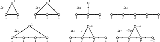
Figure 1. A few affine diagrams with balanced numbering. Choose any vertex $v$ of $\Delta_{i}$ such that $\Delta_{i}\setminus\{v\}$ is connected. Then $\Delta_{i}\setminus\{v\}$ is a root diagram for $E_{4}^{\mathcal{E}}$ if $i=1$, $E_{6}^{\mathcal{E}}$ if $i=2,3$ and $E_{8}^{\mathcal{E}}$ if $i=4,5,6,7$.

2.6 Lemma.

Let $D$ be a diagram that admits a numbering $\{n_{x}:x\in v(D)\}$ such that $y=\sum_{x\in v(D)}n_{x}.x$ is a norm zero vector of $L(D)$ and $n_{x_{j}}=1$ for some $x_{j}\in v(D)$. Then $D$ is indefinite. In particular, if $D$ admits a balanced numbering, then $D$ is indefinite.

Proof.

Suppose $K$ is an $\mathcal{E}$–root lattice with a root diagram $D_{K}$. If $D\subseteq D_{K}$, then $y=\sum_{x\in v(D)}n_{x}.x\in K$ has norm $0$. Since $K$ is positive definite, $y=0$. If $n_{x_{j}}=1$, then $x_{j}=-\sum_{x\neq x_{j}}n_{x}.x$, contradicting the fact that $v(D_{K})$ is a minimal generating set for $K$. ∎

2.7 Definition.

Let $D$ be a diagram with vertices $x_{1},\dotsb,x_{k}$ and edges $\{x_{1},x_{2}\}$, $\{x_{2},x_{3}\},\dotsb,\{x_{k-1},x_{k}\}$ and $\{x_{k},x_{1}\}$, that is, a circuit of length $k$. Changing the vectors $x_{1},\dotsb,x_{k}$ by units if necessary, we may assume that $\langle x_{i},x_{i+1}\rangle=-p$ for $1\leq i\leq k-1$ and $\langle x_{1},x_{k}\rangle=-up$ for some $u\in\mathcal{E}^{*}$. We denote this diagram by $\operatorname{Circ}_{k,u}$.

2.8 Lemma.

(a) Let $D=\operatorname{Circ}_{3,-1}$ or $D=\operatorname{Circ}_{3,\bar{\omega}}$. Then $D\simeq D_{E_{6}^{\mathcal{E}}}$.

(b) Let $D=\operatorname{Circ}_{4,\bar{\omega}}$. Then $D\simeq D_{E_{8}^{\mathcal{E}}}$.

(c) Suppose $D=\operatorname{Circ}_{k,u}$ with $k=3,4$ or $5$ but $D$ is not one of the three circuits considered in (a) and (b). Then $D$ is indefinite.

(d) Suppose $D$ is one of the diagrams given in figure 1. Then $D$ is indefinite.

Proof.

(a) Let $v(D)=\{x_{1},x_{2},x_{3}\}$. Note that $\langle x_{1},\bar{u}x_{3}\rangle=\langle x_{1},x_{2}\rangle=-p$. If we take $x_{3}^{\prime}=x_{2}-\bar{u}x_{3}$, then $\langle x_{1},x_{3}^{\prime}\rangle=0$. One checks that $\lvert x_{3}^{\prime}\rvert^{2}=6+2\operatorname{Re}(\bar{u}p)=3$ and $\langle x_{2},x_{3}^{\prime}\rangle=3+\bar{u}p\in p\mathcal{E}^{*}$, for $u=-1$ and $\bar{\omega}$. So $D$ is equivalent to the diagram $D_{E_{6}^{\mathcal{E}}}$ formed by the roots $x_{1},x_{2},x_{3}^{\prime}$.

(b) Let $x_{4}^{\prime}=\bar{\omega}x_{2}-px_{3}-x_{4}$. One checks that $x_{1},x_{2},x_{3}$ and $x_{4}^{\prime}$ form the diagram $D_{E_{8}^{\mathcal{E}}}$.

(c) For $\nu=1,\dotsb,6$, let $(n_{1,\nu},\dotsb,n_{5,\nu})$ be equal to $(1,-\omega,\bar{\omega},\bar{\omega},\bar{\omega})$, $(1,-\omega,\bar{\omega},-1,-1)$, $(1,-\omega,\bar{\omega},-1,\omega)$, $(1,-\omega,\bar{\omega},-1,\omega)$, $(1,1,1,1,1)$ and $(1,-\omega,-\omega,-\omega,-\omega)$ respectively. One checks that the vector $y=\sum_{i=1}^{k}n_{i,\nu}x_{i}$ has norm zero in $L(\operatorname{Circ}_{k,e^{2\pi i\nu/6}})$, for $k=3,4,5$ and $\nu=1,\dotsb,6$, except for the three cases considered in part (a) and (b). Part (c) now follows from lemma 2.6. Part (d) also follows from lemma 2.6. ∎

Proof of the Theorem 2.4.

Let $D$ be a root diagram for an indecomposable $\mathcal{E}$–root lattice $K$. We shall repeatedly use lemma 2.8 in two ways. First, it implies that $D$ cannot contain the diagrams mentioned in part (c) and (d) of the lemma. Secondly, from the proof of lemma 2.8, we observe the following:

If $\operatorname{Circ}_{3,u}$ or $\operatorname{Circ}_{4,u}$ is a sub-graph of $D$, then we are in one of the cases considered in part (a) or (b) of lemma 2.8 and we can change one of the vertices to get an equivalent diagram, where one of the edges has been removed. However this may introduce new edges elsewhere in the graph.

Since $K$ is indecomposable, $D$ must be connected. Let $v(D)=\{x_{1},\dotsb,x_{k}\}$. If $k=1$ (resp. $k=2$), then clearly $K\simeq E_{2}^{\mathcal{E}}$ (resp. $K\simeq E_{4}^{\mathcal{E}}$). If $k=3$, then either $D\simeq D_{E_{6}^{\mathcal{E}}}$ or $D\simeq\operatorname{Circ}_{3,u}$ with $u=-1$ or $\bar{\omega}$, which are again equivalent to $D_{E_{6}^{\mathcal{E}}}$.

Let $k=4$. We may assume that the diagram $D^{\prime}$ formed by $\{x_{1},x_{2},x_{3}\}$ is $D_{E_{6}^{\mathcal{E}}}$. If possible, suppose $D$ is not equivalent to $D_{E_{8}^{\mathcal{E}}}$. Also suppose that $\{x_{2},x_{4}\}$ is an edge of $D$. Since $D$ cannot be the affine diagram $\Delta_{3}$, either $\{x_{1},x_{2},x_{4}\}$ or $\{x_{2},x_{3},x_{4}\}$ is a circuit in $D$. Without loss, suppose $\{x_{1},x_{2},x_{4}\}$ is a circuit. Then we can change $x_{4}$ by adding a multiple of $x_{1}$ to get an equivalent diagram where $\{x_{2},x_{4}\}$ is not an edge. So $D\simeq E_{8}^{\mathcal{E}}$ or $D$ is a circuit. In the latter case, $D\simeq\operatorname{Circ}_{4,\bar{\omega}}$, since all other circuits of length $4$ are indefinite, by lemma 2.8(c). Lemma 2.8(b) implies that $\operatorname{Circ}_{4,\bar{\omega}}\simeq E_{8}^{\mathcal{E}}$.

Let $k=5$. We may assume that the diagram $D^{\prime}$ formed by $\{x_{1},x_{2},x_{3},x_{4}\}$ is $D_{E_{8}^{\mathcal{E}}}$. Since $D$ cannot be the affine diagram $\Delta_{4}$, there must be at-least two edges joining $x_{5}$ with $D^{\prime}$. Since the diagrams of the form $\operatorname{Circ}_{5,u}$ are not definite, $D$ must contain a circuit of length 3 or 4. If $\{x_{1},x_{5}\}$ is an edge, it is part of a circuit of length 3 or 4 and as before, we can remove it by shifting to an equivalent diagram. The remaining possibilities are shown in figure 2.

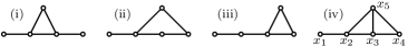
Figure 2. An undirected edge between $x_{i}$ and $x_{j}$ means $\lvert\langle x_{i},x_{j}\rangle\rvert=\lvert p\rvert$.

(The arrows on edges are not important here, so they have been omitted). In cases (iii) and (iv), we may add a multiple of $x_{3}$ to $x_{5}$ and disconnect $x_{4}$ from $x_{5}$ (note that this does not introduce an edge between $x_{1}$ and $x_{5}$). So we are reduced to the first two cases. But (i) is affine (either $\Delta_{6}$ or $\Delta_{7}$) and (ii) contains the affine diagram $\Delta_{3}$ (See figure 1). ∎

3. An attempt to characterize the diagrams for unitary reflection groups

In this section we want to address a question that was raised in [6]: How to characterize the diagrams for unitary reflection groups? We maintain the definitions and notations introduced in 1.6, 1.7 and 1.8. In 3.8-3.9, we shall describe an algorithm which, given a unitary reflection group $G$, picks out a set of reflections. As mentioned in the introduction, these reflections generate $G$ (and lift to a set of generators for $\operatorname{Braid}(G)$), if the field of definition of $G$ is $\mathbb{Q}$ or a quadratic imaginary extension of $\mathbb{Q}$. There are four fields to consider, namely, $\mathbb{Q}(\sqrt{-d})$, where $d=-1,-2,-3,-7$ and there are $12$ groups to consider. Most of these can be viewed as sets of automorphisms of certain complex lattices defined over $\mathcal{E}$ or $\mathcal{G}$, namely, $D_{4}^{\mathcal{E}},E_{6}^{\mathcal{E}},E_{8}^{\mathcal{E}},K_{10}^{\mathcal{E}},K_{12}^{\mathcal{E}}$, $D_{4}^{\mathcal{G}}$ and $E_{8}^{\mathcal{G}}$. For a description of $E_{8}^{\mathcal{E}}$, $E_{8}^{\mathcal{G}}$ and $K_{12}^{\mathcal{E}}$, see example 11b, 13b and 10a respectively, in chapter 7, section 8 of [9]). The lattice $K_{10}^{\mathcal{E}}$ is the orthogonal complement of any root in $K_{12}^{\mathcal{E}}$.

We take cue from the fact that for a Weyl group, vertices of the Dynkin diagram correspond to the simple roots, which are the positive roots having minimal inner product with a Weyl vector. Our algorithm is based on a generalization of the notion of Weyl vector.

3.1 Definition.

Let $G$ be an irreducible unitary reflection group with a root system $\Phi$ defined over $\mathcal{O}$. Let $\Phi_{*}=\Phi/\mathcal{O}^{*}$ be the set of projective roots. Given a projective root $r$, let $o(r)$ denote the order of the subgroup of $G$ generated by reflections in $r$. Let $K$ be the $\mathcal{O}$–lattice spanned by $\Phi$. Let $V$ be the complex vector space underlying $K$ and $\mathcal{M}=\cup_{r\in\Phi_{*}}r^{\bot}$ be the union of the mirrors. Define a function $\alpha:V\setminus\mathcal{M}\to V$, by

$$\alpha(w)=\sum_{r\in\Phi_{*}}o(r)^{-2}\frac{\langle r,w\rangle}{\lvert\langle r,w\rangle\rvert}\frac{r}{\lvert r\rvert}$$ (2)

3.2 Remark.

1. Note that the quantity $o(r)^{-2}\frac{\langle r,w\rangle}{\lvert\langle r,w\rangle\rvert}\frac{r}{\lvert r\rvert}$ does not change if we change $r$ by a scalar. So the function $\alpha$ is well defined and only depends on the reflection group $G$ and not on the choice of the roots. The function $\alpha$ descends to a function $\bar{\alpha}\colon\mathbb{P}(V\setminus\mathcal{M})\to\mathbb{P}(V)$. Also note that $\alpha$ is $G$–equivariant, that is, $\alpha(gw)=g\alpha(w)$ for all $g\in G$. So $\alpha$ induces a function from $\mathbb{P}(V\setminus\mathcal{M})/G$ to $\mathbb{P}(V)/G$.

2. If all the roots have the same norm, then the factor $\lvert r\rvert$ in the denominator is unnecessary and can be omitted from the definition of $\alpha$.

3. The exponent $-2$ on $o(r)$ was found by experimenting with the example $G_{26}$, which has reflections of order two and three. We have included it to indicate one of the ways in which equation (2) may be modified to possibly include other examples. If the stabilizer of each mirror has the same order, then the factor $o(r)^{-2}$ can be omitted from the definition of $\alpha$. For example, if we consider reflection group of an Euclidean root lattice (resp. $\mathcal{E}$–root lattice), then $o(r)$ is always equal to $2$ (resp. $3$).

3.3.

The case of Weyl groups: Let $W$ be a Weyl group acting on a real vector space $V_{\mathbb{R}}$ via its standard representation. Let $\mathcal{M}_{\mathbb{R}}$ be the union of the mirrors of $W$. Then $W$ can be viewed as a unitary reflection group acting on $V=V_{\mathbb{R}}\otimes\mathbb{C}$.
Claim: Let $w,w^{\prime}\in V_{\mathbb{R}}\setminus\mathcal{M}_{\mathbb{R}}$. If $w$ and $w^{\prime}$ are in the same Weyl chamber, then $\alpha(w)=\alpha(w^{\prime})$. Further, $w$ and $\alpha(w)$ belong to the same Weyl chamber. So $\alpha(w)$ is a fixed point of $\alpha$.

Proof.

The statement is invariant upon scaling $\alpha$ by a positive factor, so we do the computation omitting the factor $o(r)^{-2}=1/4$. Let $\Phi_{+}(w)$ be the set of roots having strictly positive inner product with $w$. Then $\Phi_{+}(w)$ can be chosen as a set of representatives for the projective roots, so $\alpha(w)=\sum_{r\in\Phi_{+}(w)}r/\lvert r\rvert$. Now, $w$ and $w^{\prime}$ are in the same Weyl chamber if and only if $\Phi_{+}(w)=\Phi_{+}(w^{\prime})$, so $\alpha(w)=\alpha(w^{\prime})$.

To check that $w$ and $\alpha(w)$ belong to the same Weyl chamber, first, let $\Phi$ be a root system of type $A_{n}$, $D_{n}$, $E_{6}$, $E_{7}$ or $E_{8}$. Let $w\in V_{\mathbb{R}}\setminus\mathcal{M}_{\mathbb{R}}$. Then $\rho=\tfrac{1}{2}\sum_{r\in\Phi_{+}(w)}r$ is a Weyl vector which belong to the same Weyl chamber as $w$. Note that $\alpha(w)=\sqrt{2}\rho$ and $\alpha(\sqrt{2}\rho)=\sqrt{2}\rho$.

Now consider the non-simply laced case. Since $\alpha$ is $G$–equivariant, it is enough to check that $w$ and $\alpha(w)$ are in the same Weyl chamber, for a single chamber. We show the calculation for $B_{n}$. The Weyl group of type $C_{n}$ is isomorphic to the group of type $B_{n}$. Calculations for type $G_{2}$ and $F_{4}$ are only little more complicated and will be omitted.

Let $e_{j}$ be the $j$–th unit vector in $\mathbb{Z}^{n}$. The roots of $B_{n}$ are $\{\pm e_{j},\pm e_{i}\pm e_{j}:j<i\}$. Choose $w=(w_{1},\dotsb,w_{n})$ such that $0<w_{1}<\dotsb<w_{n}$. Then $\Phi_{+}(w)=\{e_{j},e_{i}\pm e_{j}:j<i\}$. So

$$\rho^{(n)}=\alpha(w)=\sum_{r\colon\langle r,w\rangle>0}r/\lvert r\rvert=(1,1+\sqrt{2},1+2\sqrt{2},\dotsb,1+(n-1)\sqrt{2}).$$ (3)

Observe that $\rho^{(n)}$ and $w$ are in the same Weyl chamber. So $\alpha(\rho^{(n)})=\alpha(w)=\rho^{(n)}$. ∎

3.4 Definition.

Let $\Phi$ be a unitary root system defined over $\mathcal{O}$. In view of 3.3, a fixed point of $\alpha$ will be called a Weyl vector, when the root system is not defined over $\mathbb{Z}$. One may try to find a fixed point of $\alpha$ by iterating the function. Our method for selecting a set of generating reflections for $G$, is based on this notion of Weyl vector. Before describing it we show that Weyl vectors exist.

3.5 Theorem.

Let $\Phi$ be a root system for a unitary reflection group $G$. Then the function $\alpha$, defined in (2), has a fixed point.

For notational simplicity, let $\mu_{r}=\lvert r\rvert^{-1}.o(r)^{-2}$, so that,

$$\alpha(w)=\sum_{r\in\Phi_{*}}\mu_{r}\lvert\langle r,w\rangle\rvert^{-1}\langle r,w\rangle r.$$ (4)

The argument given below actually shows, that for any sequence of non-zero positive numbers $\mu_{r}$, a function of the form (4) has a fixed point. We need a lemma, which converts the problem of finding a fixed point of $\alpha$ to a maximization problem.

3.6 Lemma.

Let $\Phi$ be a unitary root system and let $\mathcal{M}$ be the union of mirrors. Consider the function $\operatorname{S}:\mathbb{P}(V)\to\mathbb{R}$, defined by

$$\operatorname{S}(w)=\lvert w\rvert^{-1}\langle\alpha(w),w\rangle=\sum_{r\in\Phi_{*}}\mu_{r}\lvert w\rvert^{-1}\lvert\langle r,w\rangle\rvert.$$ (5)

For $w\notin\mathcal{M}$, one has $\partial_{w}(\operatorname{S})=0$ if and only if $\alpha(w)=\lvert w\rvert^{-1}\operatorname{S}(w)w$. (here $\partial_{w}$ denotes the holomorphic derivative with respect to $w$).

Proof.

Let $n(w)=\langle\alpha(w),w\rangle$, so that $\operatorname{S}(w)=n(w)/\lvert w\rvert$. We fix a basis for the vector space $V$ and write $\langle r,w\rangle=r^{*}Mw$, where $r^{*}$ is the conjugate transpose of $r$ and $M$ is the matrix of the hermitian form. Differentiating, we get $\partial_{w}(\lvert\langle r,w\rangle\rvert^{2})=\langle w,r\rangle r^{*}M$. So

$$\partial_{w}(\mu_{r}\lvert\langle r,w\rangle\rvert)=\mu_{r}(2\lvert\langle r,w\rangle\rvert)^{-1}\langle w,r\rangle r^{*}M.$$

Summing over $\Phi_{*}$, one gets, $\partial_{w}n(w)=\tfrac{1}{2}\alpha(w)^{*}M$. Similarly we get $\partial_{w}(\lvert w\rvert)=\tfrac{1}{2\lvert w\rvert}w^{*}M$. It follows that

$$\partial_{w}(\operatorname{S}(w))=\partial_{w}\Bigl{(}\frac{n(w)}{\lvert w\rvert}\Bigr{)}=\frac{\tfrac{1}{2}\lvert w\rvert\alpha(w)^{*}M-\tfrac{1}{2\lvert w\rvert}n(w)w^{*}M}{\lvert w\rvert^{2}}=\frac{\alpha(w)^{*}-\frac{\operatorname{S}(w)}{\lvert w\rvert}w^{*}}{2\lvert w\rvert}M.$$

Since $M$ is an invertible matrix, the lemma follows. ∎

Proof of Theorem 3.5.

We first prove the following claim:
Claim: If $w\in V$ lies on a mirror, then the function $\operatorname{S}$ can not have a local maximum at $w$.
Fix a root $r_{0}\in\Phi$ and $w\in r_{0}^{\bot}$. Assume $\lvert w\rvert=1$. Take $w^{\prime}=w+\epsilon\xi r_{0}$ , where $\xi$ is a complex root of unity and $\epsilon$ is a small positive real number so that $\epsilon^{2}$ is negligible. We shall show that $\operatorname{S}(w^{\prime})>\operatorname{S}(w)$, for suitable choice of $\xi$. Ignoring terms of order $\epsilon^{2}$, we have $\lvert w^{\prime}\rvert^{2}=\lvert w\rvert^{2}+2\operatorname{Re}(\epsilon\langle w,r_{0}\rangle)=\lvert w\rvert^{2}=1$. Let $\Psi_{0}=\Phi_{*}\cap w^{\bot}$ and $\Psi_{1}=\Phi_{*}\setminus\Psi_{0}$. Then

$$\operatorname{S}(w^{\prime})=\sum_{r\in\Psi_{0}}\mu_{r}\lvert\langle r,w^{\prime}\rangle\rvert+\sum_{r\in\Psi_{1}}\mu_{r}\lvert\langle r,w^{\prime}\rangle\rvert=\epsilon\sum_{\Psi_{0}}\mu_{r}\lvert\langle r,r_{0}\rangle\rvert+\sum_{\Psi_{1}}\mu_{r}\bigl{|}\langle r,w\rangle+\epsilon\xi\langle r,r_{0}\rangle\bigr{|}.$$

Let $a=\langle r,w\rangle\neq 0$ and $b=\xi\langle r,r_{0}\rangle$. Using the first order expansion of $(1+x)^{1/2}$, we have,

$$\lvert a+\epsilon b\rvert=\sqrt{\lvert a\rvert^{2}+2\operatorname{Re}(\epsilon b\bar{a})}=\lvert a\rvert+\operatorname{Re}(\epsilon b\bar{a}\lvert a\rvert^{-1}).$$

It follows that

$$\operatorname{S}(w^{\prime})=\operatorname{S}(w)+\epsilon\sum_{\Psi_{0}}\mu_{r}\lvert\langle r,r_{0}\rangle\rvert+\epsilon\operatorname{Re}\Bigl{(}\xi\sum_{\Psi_{1}}\mu_{r}\langle r,r_{0}\rangle\overline{\langle r,w\rangle}\lvert\langle r,w\rangle\rvert^{-1}\Bigr{)}.$$

Note that the third term can be made non-negative by choosing $\xi$ suitably, and the second term is positive, since $r_{0}\in\Psi_{0}$. This proves the claim.

The function $\operatorname{S}$ is continuous on $\mathbb{P}(V)$, so it attains its global maximum, say at $w_{0}$. The claim we just proved implies that $w_{0}\notin\mathcal{M}$, so $\partial_{w_{0}}(\operatorname{S})=0$. Let $w_{1}=\lvert w_{0}\rvert^{-1}\operatorname{S}(w_{0})w_{0}$. Lemma 3.6 implies that $\alpha(w_{1})=\alpha(w_{0})=w_{1}$. ∎

3.7 Definition.

Let $(\mathcal{O},G,\Phi,K,V)$ be as in 3.1. Given $w\in V$, let $(r_{1},\dotsb,r_{N})$ be the projective roots of $G$ arranged so that $d(r_{1}^{\bot},w)\leq\dotsb\leq d(r_{N}^{\bot},w)$, where $d$ is the Fubini-Study metric on $\mathbb{P}(V)$. So

$$d(r^{\bot},w)=\sin^{-1}(\lvert\langle r,w\rangle\rvert/\lvert r\rvert\lvert w\rvert).$$

Let $k$ be the minimum number of reflections needed to generate $G$. Define $\Delta(w)=\{r_{1},\dotsb,r_{k}\}$. In other words, $\Delta(w)$ consists of $k$ projective roots, whose mirrors are closest to $w$.

3.8.

Method to obtain a set of “simple reflections”: We now describe a computational procedure in which, the input is a unitary reflection group $G$, (or equivalently, a projective root system $\Phi_{*}$ for $G$ and the numbers $\{o(r)\colon r\in\Phi_{*}\}$) and the output is either the empty set or a non-empty set of projective roots, to be called the simple roots. The reflections in the simple roots are called simple reflections. A set of simple reflections form a simple system.

1. From the set $\{w\colon\alpha(w)=w\}$, choose $w$ such that $\operatorname{S}(w)$, defined in (5), is maximum.

2. Let $\Delta(w)=\{r_{1},r_{2},\dotsb,r_{k}\}$.

3. If $r_{1},\dotsb,r_{k}$ are linearly dependent, then return the empty set.

4. If $r_{1},\dotsb,r_{k}$ are linearly independent, then return $\Delta(w)$ (the simple roots).

In practice, for each group $G$ to be studied, we execute the following algorithm many times.

3.9.

Algorithm: Start with a random vector $w_{0}\in V$. Generate a sequence $w_{n}$ by $w_{n}=\alpha(w_{n-1})$. If the sequence stabilizes, then say that the algorithm converges and let $w=\lim w_{n}$. Note down $\Delta(w)$ and $\operatorname{S}(w)$.

For computer calculation, we assume that $w_{n}$ stabilizes if $\lvert w_{n+1}-w_{n}\rvert^{2}/\lvert w_{n}\rvert^{2}$ becomes small, say less than $10^{-8}$, and remains small and decreasing for many successive values of $n$. Note that if $\alpha(w)=w$, then $\operatorname{S}(w)=\lvert w\rvert$. From the values of $\operatorname{S}(w)$, the maximum, denoted by $\operatorname{S}_{\mathrm{max}}^{G}$, can be found. (In all the examples that we have studied, $\operatorname{S}(w)$ takes at-most two values on the set of fixed points of $\alpha$ found experimentally, so finding the maximum is not difficult). Each instance of the algorithm, that produced a vector $w$ with $\operatorname{S}(w)=\operatorname{S}_{\mathrm{max}}^{G}$, now yields a simple system $\Delta(w)$ provided that $\Delta(w)$ is a linearly independent set.

3.10.

Observations for Weyl groups: First, suppose that $\Phi$ is a root system for a Weyl group $W$. We maintain the notations of 3.3 and ignore the factor $o(r)^{-2}=\tfrac{1}{4}$ in the definition of $\alpha$. Given $w\in V_{\mathbb{R}}$, let $\delta_{w}(r)=\lvert\langle r,w\rangle\rvert/\lvert r\rvert$. Arranging the roots according to increasing distance from $w$ (according to the spherical metric or the Fubini-Study metric) is equivalent to arranging them according to increasing order of $\delta_{w}(r)$.
Claim: Let $W$ be a Weyl group, $w_{0}\in V_{\mathbb{R}}\setminus\mathcal{M}_{\mathbb{R}}$ and $w=\alpha(w_{0})$. Then the algorithm 3.9 converges in one iteration and yields a simple system $\Delta(w)$. For Weyl groups, the definition of a set of simple roots given in 3.8 agrees with the classical notion. Further, for each simple root $r\in\Delta(w)$, we have $\delta_{w}(r)=1$. So the simple mirrors are equidistant from $w$.

Proof.

We saw in 3.3 that $w=\alpha(w_{0})$ is a fixed point of $\alpha$, so $w=\alpha(w_{0})=\alpha^{2}(w_{0})=\dotsb$, that is, the algorithm converges in one iteration.

Suppose $\Phi$ is a root system of type $A$, $D$ or $E$. Then $w=\alpha(w_{0})=\sqrt{2}\rho$, where $\rho$ is a Weyl vector. So $\Delta(w)=\Delta(\rho)$ consists of a set of simple roots and for each $r\in\Delta(w)$, one has $\langle r,\rho\rangle=1$, so $\delta_{w}(r)=1$.

In type $B_{n}$, if $w_{0}$ is in the Weyl chamber containing the vector $\rho^{(n)}$ given in equation (3), then one has $w=\rho^{(n)}=\alpha(\rho^{(n)})=\dotsb$. Observe that the function $\delta_{w}(r)$ attains its minimum for the simple roots $\Delta(w)=\{e_{1},e_{2}-e_{1},\dotsb,e_{n}-e_{n-1}\}$ and $\delta(r)=1$ for each $r\in\Delta(w)$. The claim was verified for $G_{2}$ and $F_{4}$ without difficulty. ∎

3.11.

Observations for complex root systems: In the following discussion, let $G$ be one of the unitary reflection groups from the set $\{G_{4},G_{5},G_{25},G_{26},G_{32},G_{33},G_{34}\}\cup\{G_{8},G_{29},G_{31}\}\cup\{G_{12}\}\cup\{G_{24}\}$. The groups given in four subsets are defined over $\mathbb{Q}(\sqrt{-3})$, $\mathbb{Q}(\sqrt{-1})$, $\mathbb{Q}(\sqrt{-2})$ and $\mathbb{Q}(\sqrt{-7})$ respectively. In each case, a projective root system $\Phi_{*}(G)$ for $G$ is chosen. These are described in the appendix A. For each of these groups $G$, we have run algorithm 3.9 at-least one thousand times and obtained many simple systems by method 3.8. The calculations were performed using the GP/PARI calculator. The main observations made from the computer experiments are the following:

The sequence $\{w_{n}\}$ stabilizes in each trial for each $G$ mentioned above. The simple reflections generate $G$ and satisfy the same set of relations $R_{G}$, every time. In other words, the simple roots form the same “diagram” every time. For $G_{4}$, $G_{5}$, $G_{8}$, $G_{25}$, $G_{26}$, $G_{32}$, these are Coxeter’s diagrams, (see [6]). For $G_{24}$, the relations $R_{G}$ are given in A.5 (this is the third presentation given in [5]). For $G_{29}$, $G_{31}$, $G_{33}$ and $G_{34}$ new diagrams are obtained. These diagrams are given in figure 3 and corresponding presentations for the braid groups are given in 4.5, 4.6. Finally, for $G_{12}$ a presentation is given in A.4.

Further observations from the computer experiments are summarized below.

1. If $G$ is not $G_{29}$, $G_{31}$ or $G_{32}$, then for all $w$ such that $\alpha(w)=w$, the function $S(w)$ attains the same value. So each trial of the algorithm yields a maxima $w$ for $\operatorname{S}$. For $G_{29}$, $G_{31}$ and $G_{32}$, the function $\operatorname{S}(w)$ attains two values on the fixed point set of $\alpha$. In these three cases, the $\mathbb{Z}$–span of the roots form the $E_{8}$ lattice.

2. If $G\neq G_{33}$ and $G$ is well generated, then in each trial of the algorithm, we find that the vectors $\{r_{1},\dotsb,r_{k}\}$ are linearly independent. So each choice of a maxima $w$ for the function $\operatorname{S}$ yields a set of simple roots $\Delta(w)$. For $G_{33}=R(K_{10}^{\mathcal{E}})$, in most of the trials, we find that $\{r_{1},\dotsb,r_{5}\}$ are linearly dependent. So most trials do not yield a set of simple roots $\Delta(w)$. In an experiment with $5000$ trials, only $297$ yielded simple systems.

3. Let $G\in\{G_{33},G_{34},G_{29}\}$. These are the three well generated groups for which the diagrams obtained by method 3.8 are different from the ones in the literature. Let $g_{1},\dotsb,g_{k}$ be a set of simple reflections of $G$ obtained by method 3.8. For these three groups, we have verified the following result. (almost a re-statement of 1.2):
   
   Fix a permutation $\pi$ so that the order of the product $p=g_{\pi_{1}}\dotsb g_{\pi_{k}}$ is maximum (over all permutations). Then, the order of $p$ is equal to the Coxeter number of $G$ (denoted by $h$) and the eigenvalues of either $p$ or $p^{-1}$ are $e^{2\pi i(d_{1}-1)/h},\dotsb,e^{2\pi i(d_{k}-1)/h}$, where $d_{1},\dotsb,d_{k}$ are the invariant degrees of $G$.
   
   The invariant degrees of $G_{29}$, $G_{33}$ and $G_{34}$ are $(4,8,12,20)$, $(4,6,10,12,18)$ and $(6,12,18,24,30,42)$ respectively. In all three cases, $h$ is equal to the maximum degree.

4. Start with $w_{0}\in V$ and consider the sequence defined by $w_{n}=\alpha(w_{n-1})$. Roughly speaking, each iteration of the function $\alpha$ makes the vector $w_{n}$ more symmetric with respect to the set of projective roots $\Phi_{*}$. The function $\operatorname{S}$ measures this symmetry. So the fixed points $w$ of $\alpha$ are often the vectors that are most symmetrically located with respect to $\Phi_{*}$.

   Based on the above discussion, an alternative definition of a Weyl vector may be suggested, namely, a vector $w\in V$, such that $d(w,\mathcal{M})$ is maximum. (This was suggested to me by Daniel Allcock). It seems harder to compute these vectors, so we have not experimented much with this alternative definition. However, we would like to remark that for some complex and quaternionic Lorentzian lattices, similar analogs of Weyl vectors and simple roots, are useful. (One such example is studied in [3]; other examples are studied in [2]. In these examples of complex and quaternionic Lorentzian lattices, the simple roots are again defined as those whose mirrors are closest to the “Weyl vector”.)

5. The method 3.8 fails for the primitive unitary reflection groups that are not defined over $\mathbb{Q}$ or a imaginary quadratic extension of $\mathbb{Q}$ and for the imprimitive groups $G(de,e,n)$, except when they are defined over $\mathbb{Q}$, that is, for the cases $G(1,1,n+1)\simeq A_{n}$, $G(2,1,n)\simeq BC_{n}$ and $G(2,2,n)\simeq D_{n}$. It fails in the sense that the set $\Delta(w)$ does not in general form a minimal set of generators for the group. This was found by experimenting with $G(de,e,n)$ for small values of $(d,e,n)$ and also with $G_{6}$ and $G_{9}$ (see appendix A.4). Although method 3.8 fails, the following observation holds for $G(de,e,n)$:

   Let $k$ be the minimum number of reflections needed to generate $G(de,e,n)$ ($k=n$ or $n+1$). There exists a vector $w\in V$ such that, if $r_{1}^{\bot},\dotsb,r_{k}^{\bot}$ are the mirrors closest to $w$, then reflections in $\{r_{1},\dotsb,r_{k}\}$ generate $G(de,e,n)$.

   For $G(de,e,n)$, one can take $w=\rho^{(n)}$ (the vector we obtained for the Weyl group $B_{n}$; see equation (3)). It is easy to check that $\Delta(\rho^{(n)})$ forms the known diagrams for $G(de,e,n)$. We found $\rho^{(n)}$ by using an algorithm that tries to find a point in $V$ whose distance from $\mathcal{M}$ is at a local maximum. For small values of $d$, $e$ and $n$, we find that this algorithm always converge to $\rho^{(n)}$.

4. The braid groups for $G_{29}$, $G_{31}$, $G_{33}$, $G_{34}$.

4.1.

For this section, let $N\in\{29,31,33,34\}$. Algorithm 3.9, applied to $G_{N}$, yields new diagrams, denoted by $D_{N}$ (see figure 3). Before stating the main result, proposition 4.6, we need some notations.

4.2.

Notations: Let $\{x_{i}\colon i\in\mathbb{Z}/k\mathbb{Z}\}$ be elements of a monoid $M$. Let $\mathcal{C}_{m}\langle x_{0},\dotsb,x_{k-1}\rangle$ denote the positive and homogeneous relation

$$x_{0}x_{1}\dotsb x_{m-1}=x_{1}x_{2}\dotsb x_{m}.$$ (6)

For example $\mathcal{C}_{2}\langle a,b\rangle$ (resp. $\mathcal{C}_{3}\langle a,b\rangle$) says that $a$ and $b$ commutes (resp. braids); while $\mathcal{C}_{5}\langle a,b\rangle$ (resp. $\mathcal{C}_{4}\langle a,b,c\rangle$) stands for the relation $ababa=babab$ and (resp. $abca=bcab$). If $x,y$ are elements in a group, let $c_{x}(y):=xyx^{-1}$.

Given a diagram $D$ (such as in figure 3) let $\operatorname{Cox}(D,\infty)$ be the group defined by generators and relations as follows: The generators of $\operatorname{Cox}(D,\infty)$ correspond to the vertices of $D$. The relations are encoded by the edges of $D$: $k$ edges between vertices $p$ and $q$ encodes the relation $\mathcal{C}_{k+2}\langle p,q\rangle$. In particular, no edge between $p$ and $q$ indicates that $p$ and $q$ commute, while an edge marked with $\infty$ indicates that $\operatorname{Cox}(D,\infty)$ has no defining relation involving only the generators $p$ and $q$. Let $\operatorname{Cox}(D,n)$ be the quotient of $\operatorname{Cox}(D,\infty)$ obtained by imposing the relation $p^{n}=1$ for each vertex $p$ of $D$. Let $\operatorname{Cox.Rel}(D)$ be the defining relations of $\operatorname{Cox}(D,\infty)$.

Let $\tilde{A}_{n}$ denote the affine Dynkin diagram of type $A_{n}$. (Picture it as a regular polygon with $(n+1)$ vertices). Fix an automorphism $\rho$ of $\tilde{A}_{n}$ (hence of $\operatorname{Cox}(\tilde{A}_{n},\infty)$), that rotates the Dynkin diagram $\tilde{A}_{n}$ by an angle $2\pi/n$. Let $x$ be a vertex of $\tilde{A}_{n}$. We say that the relation $\mathcal{C}_{m}\langle x,\rho(x),\dotsb,\rho^{n}(x)\rangle$ is cyclic in $\operatorname{Cox}(\tilde{A}_{n},\infty)$ if the relation $\mathcal{C}_{m}\langle\rho(x),\dotsb,\rho^{n}(x),x\rangle$ holds in the quotient $\operatorname{Cox}(\tilde{A}_{n},\infty)/\langle\mathcal{C}_{m}\langle x,\rho(x),\dotsb,\rho^{n}(x)\rangle\rangle$ (so $\mathcal{C}_{m}\langle y,\rho(y),\dotsb,\rho^{n}(y)\rangle$ holds for each vertex $y\in\tilde{A}_{n}$).

The two lemmas stated below help us verify proposition 4.6. But these might be of independent interest for studying groups satisfying relations of the form (6). The proofs are straight-forward and given in B.2 and B.3. It is easy to write down more general statements than those stated below and give an uniform proof, at-least for Lemma 4.4. To keep things simple, we have resisted this impulse to generalize.

4.3 Lemma.

Let $(x_{0},\dotsb,x_{n})=(x,\rho(x),\dotsb,\rho^{n}(x))$ be the vertices of $\tilde{A}_{n}$.

(a) $\mathcal{C}_{n}\langle x_{0},\dotsb,x_{n}\rangle$ is cyclic in $\operatorname{Cox}(\tilde{A}_{n},\infty)$ for all $n$.

(b) $\mathcal{C}_{n+2}\langle x_{0},\dotsb,x_{n}\rangle$ (resp. $\mathcal{C}_{2n+2}\langle x_{0},\dotsb,x_{n}\rangle$) is cyclic in $\operatorname{Cox}(\tilde{A}_{n},\infty)$ if and only if $x_{n}=x_{2}$ (resp. $x_{n-1}=x_{1}$). In particular $\mathcal{C}_{4}\langle x_{0},x_{1},x_{2}\rangle$ and $\mathcal{C}_{6}\langle x_{0},x_{1},x_{2}\rangle$ are cyclic in $\operatorname{Cox}(\tilde{A}_{2},\infty)$.

(c) Let $n>2$. Then $\mathcal{C}_{2n+3}\langle x_{0},\dotsb,x_{n}\rangle$ is cyclic in $\operatorname{Cox}(\tilde{A}_{n},\infty)$ if and only if $x_{n-1}=x_{2}$. In particular $\mathcal{C}_{9}\langle x_{0},x_{1},x_{2},x_{3}\rangle$ is cyclic in $\operatorname{Cox}(\tilde{A}_{3},\infty)$.

4.4 Lemma.

(a) Assume $x$ braids with $y$ in a group $G$. Then the following are equivalent:

(i) $\mathcal{C}_{4}\langle x,y,z\rangle$ (ii) $c_{x}(y)$ commutes with $z$. (iii) $c_{y}(z)$ commutes with $x$.

If $x$ also braids with $z$ then (i),(ii), (iii) are equivalent to (iv): $c_{z}(x)$ commutes with $y$.

(b) Assume $x$ braids with $y$ and $z$ in a group $G$. Then the following are equivalent:

(i) $\mathcal{C}_{6}\langle x,y,z\rangle$ (ii) $c_{x}(y)$ braids with $z$. (iii) $c_{y}(z)$ braids with $x$. (iv) $c_{z}(x)$ braids with $y$.

(c) Suppose $x,y,z,w$ are the Coxeter generators of $\operatorname{Cox}(\tilde{A}_{3},\infty)$. Then $\mathcal{C}_{9}\langle x,y,z,w\rangle$ holds if and only if $c_{xy}(z)$ braids with $w$.

4.5.

The relations: Let $N\in\{29,31,33,34\}$. The vertices of the diagram $D_{N}$ and $D^{\prime}_{N}$ given in figure 3 correspond to generators of $\operatorname{Braid}(G_{N})$. The edges indicate the Coxeter relations. However some more relations are needed to obtain a presentation of $\operatorname{Braid}(G_{N})$. These relations are given below. All of them are of the form (6).

$$E_{34} =\{\mathcal{C}_{4}\langle a_{2},a_{3},a_{4}\rangle,\mathcal{C}_{4}\langle a_{3},a_{4},a_{5}\rangle,\mathcal{C}_{9}\langle a_{3},a_{2},a_{1},a_{5}\rangle,$$

$$\;\;\;\;\;\;\;\;\mathcal{C}_{4}\langle a_{2},a_{1},a_{6}\rangle,\mathcal{C}_{4}\langle a_{2},a_{3},a_{6}\rangle,\mathcal{C}_{9}\langle a_{1},a_{5},a_{3},a_{6}\rangle\},\;\;\;\;\;\;\;\;\;E^{\prime}_{34}=\{\mathcal{C}_{6}\langle t,u,w\rangle\},$$

$$E_{29} =\{\mathcal{C}_{4}\langle a_{4},a_{2},a_{1}\rangle,\mathcal{C}_{4}\langle a_{3},a_{1},a_{4}\rangle,\mathcal{C}_{6}\langle a_{3},a_{1},a_{2}\rangle\},\;\;\;\;\;\;\;\;\;\;\;\;\;\;\;\;E^{\prime}_{29}=\{\mathcal{C}_{6}\langle u,t,v\rangle\},$$

$$E_{31} =\{\mathcal{C}_{4}\langle a_{4},a_{2},a_{1}\rangle,\;\;\mathcal{C}_{6}\langle a_{2},a_{3},a_{4}\rangle,\mathcal{C}_{3}\langle a_{3},a_{5},a_{4}\rangle,$$

$$\mathcal{C}_{3}\langle a_{5},a_{4},a_{3}\rangle,\mathcal{C}_{4}\langle a_{1},a_{5},a_{2}\rangle,\mathcal{C}_{4}\langle a_{3},a_{1},a_{4}\rangle,\mathcal{C}_{4}\langle a_{4},a_{2},a_{5}\rangle\},\;\;E^{\prime}_{31}=\{\mathcal{C}_{3}\langle s,u,w\rangle,\mathcal{C}_{3}\langle u,w,s\rangle\}.$$

Let $E_{33}$ (resp. $E^{\prime}_{33})$ be the relations in $E_{34}$ (resp. $E^{\prime}_{34}$) that does not involve $a_{6}$ (resp. $x$). Let $R_{N}=\operatorname{Cox.Rel}(D_{N})\cup E_{N}$ and $R^{\prime}_{N}=\operatorname{Cox.Rel}(D^{\prime}_{N})\cup E^{\prime}_{N}$. Let $B_{N}$ (resp. $B^{\prime}_{N}$) be the group generated by the vertices of the diagram $D_{N}$ (resp. $D^{\prime}_{N}$) satisfying the relations $R_{N}$ (resp. $R^{\prime}_{N}$). It was conjectured in [5] and proved in [4] that $\operatorname{Braid}(G_{N})\simeq B^{\prime}_{N}$.

Figure 3. Let $D_{33}=D_{34}\setminus\{a_{6}\}$ and $D^{\prime}_{33}=D^{\prime}_{34}\setminus\{x\}$. The diagrams $D_{N}$ and $D^{\prime}_{N}$ encode presentations for $\operatorname{Braid}(G_{N})$.

4.6 Proposition.

Assume the setup given in 4.5. The presentations $B_{N}$ and $B^{\prime}_{N}$ are equivalent. So $B_{N}$ gives a presentation of $\operatorname{Braid}(G_{N})$. The quotient of $B_{N}$ obtained by imposing the relations $a_{i}^{2}=1$, for all $i$, is isomorphic to $G_{N}$.

sketch of proof.

We define the maps $\varphi_{N}:B^{\prime}_{N}\to B_{N}$ and $\psi_{N}:B_{N}\to B^{\prime}_{N}$ on the generators. Let

$$\varphi_{29}:(s,t,v,u)\mapsto(c_{(a_{2}a_{3}a_{1})^{-1}}(a_{4}),a_{1},a_{2},a_{3}),\;\;\;\;\psi_{29}:(a_{1},a_{2},a_{3},a_{4})\mapsto(t,v,u,c_{vut}(s)).$$

$$\varphi_{31}:(s,t,u,w,v)\mapsto(a_{5},a_{1},a_{3},c_{a_{3}^{-1}}(a_{4}),c_{a_{4}}(a_{2})),$$

$$\psi_{31}:(a_{5},a_{1},a_{3},a_{4},a_{2})\mapsto(s,t,u,c_{u}(w),c_{uw^{-1}u^{-1}}(v)).$$

$$\varphi_{34}:(s,t,u,v,w)\mapsto(a_{1},a_{2},a_{3},c_{a_{3}}(a_{4}),c_{a_{2}a_{1}}(a_{5}),c_{a_{4}a_{2}a_{1}a_{5}a_{3}}(a_{6})),$$

$$\psi_{34}:(a_{1},a_{2},a_{3},a_{4},a_{5})\mapsto(s,t,u,c_{u^{-1}}(v),c_{(ts)^{-1}}(w),c_{(vuwtsu)^{-1}}(x)).$$

Let $\varphi_{33}$ and $\psi_{33}$ be the restrictions of $\varphi_{34}$ and $\psi_{34}$ respectively.

To check that $\varphi_{N}$ (resp. $\psi_{N}$) is a well defined group homomorphism, we have to verify that $(\varphi_{N}(s),\varphi_{N}(t),\dotsb,)$ (resp. $(\psi_{N}(a_{1}),\psi_{N}(a_{2}),\dotsb)$) satisfy the relations $R^{\prime}_{N}$ (resp. $R_{N}$). This verification was done by hand using lemmas 4.3 and 4.4. The details, given in B.5, B.6 and B.7, are rather tedious. It is easy to see that $\varphi_{N}$ and $\psi_{N}$ are mutual inverses, so $B_{N}\simeq B^{\prime}_{N}$.

The generators $a_{i}$ for $B_{N}$ were found as follows. We first found generators $\bar{a}_{i}$ of order $2$ in $G_{N}$ using algorithm 3.9 and then let $a_{i}$ be a lift of $\bar{a}_{i}$, that is, we chose $R_{N}$ to be an appropriate subset of the relations satisfied by $\{\bar{a}_{1},\bar{a}_{2},\dotsb\}$ in $G_{N}$. So, from our construction, we know that there are reflections of order $2$ in $G_{N}$ that satisfy the relations $R_{N}$, that is, $G_{N}$ is a quotient of $\bar{B}_{N}:=B_{N}/\langle a_{i}^{2}=1\text{\; for all \;}i\rangle$. Using coset enumeration on the computer algebra system MAGMA, we verified that $\bar{B}_{N}$ has the same order as $G_{N}$. ∎

4.7 Remark.

Here are some concluding remarks for this section.

1. The transformations, $\varphi_{N}$ and $\psi_{N}$, given in the proof of 4.6 were found first by computing inside the reflection group $G_{N}$ and then choosing appropriate lifts to $\operatorname{Braid}(G)$.

2. It is interesting to note that all the relations encountered in the presentations of the braid groups of type $G_{33}$ and $G_{34}$ are cyclic relations (see 4.3) of the form $\mathcal{C}_{n}\langle x_{1},\dotsb,x_{m}\rangle$ where $x_{1},\dotsb,x_{m}$ is a minimal cycle (actually a triangle or a square) inside the diagrams.

3. The relation $\mathcal{C}_{9}\langle a_{4},a_{2},a_{1},a_{5}\rangle$ (resp. $\mathcal{C}_{6}\langle a_{2},a_{3},a_{4}\rangle$) hold as a consequence of the relations $R_{33}$ (resp. $R_{29}$) (see B.8). So the content of Prop. 4.6 for $N=29,33$ and $34$ can be succinctly stated as follows: The relations needed to present $\operatorname{Braid}(G_{N})$ are $\operatorname{Cox.Rel}(D_{N})$ and one relation of the form $\mathcal{C}_{n}\langle x_{1},\dotsb,x_{m}\rangle$ for each minimal cycle $x_{1},\dotsb,x_{m}$ in $D_{N}$. Further, this $n$ is the smallest integer for which the relation $\mathcal{C}_{n}\langle x_{1},\dotsb,x_{m}\rangle$ holds in $G_{N}$. It might be interesting to find out all the unitary reflection groups for which a similar statement is true.

4. The situation with the non-well generated group $G_{31}$ is not as nice. First of all, we were not able to verify the previous remark for $\operatorname{Braid}(G_{31})$. Further, deleting the relations involving $a_{5}$ from $R_{31}$ only yields a proper subset of $R_{29}$. The problem is that the relations $\mathcal{C}_{4}\langle a_{1},a_{2}\rangle,\mathcal{C}_{4}\langle a_{1},a_{4}\rangle,\mathcal{C}_{4}\langle a_{2},a_{5}\rangle,\mathcal{C}_{4}\langle a_{3},a_{4}\rangle,\mathcal{C}_{4}\langle a_{3},a_{5}\rangle,\mathcal{C}_{4}\langle a_{4},a_{5}\rangle$ hold in $G_{31}$, but we were not able to check whether these relations are implied by $R_{31}$. This would be equivalent to checking whether the relations $\mathcal{C}_{4}\langle s,u\rangle,\mathcal{C}_{4}\langle u,w\rangle,\mathcal{C}_{4}\langle s,w\rangle$ are implied by $R^{\prime}_{31}$.

5. Some relations of the form $\mathcal{C}_{k}\langle x_{0},\dotsb,x_{n}\rangle$ were studied in [8]. Conway called them deflation relations, because they often “deflate” infinite Coxeter groups to finite groups. The groups studied in this section provide some examples of this. We mention two other examples: (i) the quotient of the affine Weyl group $\operatorname{Cox}(\tilde{A}_{n},2)$ obtained by the adding the cyclic (see 4.3(a)) relation $\mathcal{C}_{n}\langle x_{0},\dotsb,x_{n}\rangle$ is the finite Weyl group $\operatorname{Cox}(A_{n},2)$. (ii) There is a graph $D$ with $26$ vertices such that the quotient of the infinite Coxeter group $\operatorname{Cox}(D,2)$ obtained by adding the cyclic deflation relations $\mathcal{C}_{11}\langle x_{0},\dotsb,x_{10}\rangle$, for each minimal cycle with $12$ vertices in $D$, is the wreath product of the monster simple group with $\mathbb{Z}/2\mathbb{Z}$ (see [8]).

5. the affine reflection groups

5.1.

In this section we shall describe affine diagrams for the primitive unitary reflection groups defined over $\mathcal{E}$, except for $G_{5}$. (Including $G_{5}$ would further complicate notations). An affine diagram is obtained by adding an extra node to the corresponding “unitary diagram”. Each affine diagram admits a balanced numbering. A unitary diagram can be extended to an affine diagram in many ways. We have chosen one that makes the diagram more symmetric. The Weyl vector, that yielded the unitary diagram, is often fixed by the affine diagram automorphisms.

The discussion below and the lemma following it are direct analogs of the corresponding results for Euclidean root lattices. We have included a proof since we could not find a convenient reference.

Let $\Phi$ be a unitary root system defined over $\mathcal{E}$, for an unitary reflection group $G$. Let $K$ be the $\mathcal{E}$–lattice spanned by $\Phi$. Assume that the subgroup of $\operatorname{Aut}(K)$ generated by reflections in $\Phi$ is equal to $G$. Let $\mathcal{E}_{0}$ be the one dimensional free module over $\mathcal{E}$ with zero hermitian form. Let $\tilde{K}=K\oplus\mathcal{E}_{0}$. Let us write the elements of $\tilde{K}$ in the form $(y,m)$ with $y\in K$ and $m\in\mathcal{E}$. Let $\tilde{G}$ be the subgroup of $\operatorname{Aut}(\tilde{K})$ generated by reflections in $\tilde{\Phi}=\{(x,m)\colon x\in\Phi,m\in\mathcal{E}\}$. Note that $\phi_{(x,m)}^{\omega}\in\tilde{G}$ if and only if $\phi_{x}^{\omega}\in G$. Consider the semi-direct product $K\rtimes G$, in which the product is defined by $(x,g).(y,h)=(x+gy,gh)$. The faithful action of $K\rtimes G$ on $K$ via affine transformations is given by $(x,g)y=x+gy$.

5.2 Lemma.

Given the setup above, assume that $\lvert r\rvert^{2}=3$ for all $r\in\Phi$ and $K^{\prime}\supseteq p^{-1}K$.

(a) The affine reflection group $\tilde{G}$ is isomorphic to the semi-direct product $K\rtimes G$.

(b) Let $r_{0}$ be a root of $\Phi$ such that the orbit $Gr_{0}$ spans $K$ as a $\mathbb{Z}$–module. If $\phi^{\omega}_{r_{1}},\dotsb,\phi^{\omega}_{r_{k}}$ generate $G$, then $\phi^{\omega}_{(r_{1},0)},\dotsb,\phi^{\omega}_{(r_{k},0)}$, together with $\phi^{\omega}_{(r_{0},1)}$ generate $\tilde{G}$.

(c) If $\phi^{\omega}_{r_{0}}$ commutes (resp. braids) with $\phi^{\omega}_{r_{j}}$, then $\phi^{\omega}_{(r_{0},1)}$ commutes (resp. braids) with $\phi^{\omega}_{(r_{j},0)}$.

Proof.

(a) Identify $K$ (resp. $G$) inside $\tilde{K}$ (resp. $\tilde{G}$) via $y\mapsto(y,0)$ (resp. $\phi^{\omega}_{x}\mapsto\phi^{\omega}_{(x,0)}$ ). Recall $p=2+\omega$. For $x\in K$, define

$$t_{x}(y,n)=(y,n-p^{-1}\langle x,y\rangle).$$ (7)

The automorphisms $t_{x}$ of $\tilde{K}$ are called translations. The subgroup of $\operatorname{Aut}(\tilde{K})$ generated by translations is isomorphic to the additive group of $K$. For any root $(x,m)\in\tilde{\Phi}$, one has,

$$\phi_{(x,m)}^{\omega}(y,n)=(\phi_{x}^{\omega}(y),n-mp^{-1}\langle x,y\rangle)=\phi_{(x,0)}^{\omega}\circ t_{\bar{m}x}(y,n).$$

Let us write $\phi^{\omega}_{(x,0)}=\phi^{\omega}_{x}$. From the above equation, one has, in particular,

$$t_{x}=(\phi^{\omega}_{x})^{-1}\circ\phi^{\omega}_{(x,1)}.$$ (8)

From equation (8), it follows that $\phi^{\omega}_{a}t_{x}(\phi^{\omega}_{a})^{-1}=t_{\phi^{\omega}_{a}(x)}$. So $(x,g)\mapsto t_{x}\circ g$ is an isomorphism from $K\rtimes G$ onto $\tilde{G}$.

(b) Let $G_{1}$ be the subgroup of $\tilde{G}$ generated by $\phi^{\omega}_{r_{1}},\dotsb,\phi^{\omega}_{r_{k}}$ and $\phi^{\omega}_{(r_{0},1)}$. Then $G\subseteq G_{1}$. Let $x=gr_{0}$ be a root in the $G$–orbit of $r_{0}$. Then $t_{x}=(\phi^{\omega}_{x})^{-1}\phi^{\omega}_{(x,1)}=(\phi^{\omega}_{x})^{-1}g\phi^{\omega}_{(r_{0},1)}g^{-1}\in G_{1}$. Since the roots in the $G$–orbit of $r_{0}$ span $K$ as a $\mathbb{Z}$–module, it follows that $t_{x}\in G_{1}$ for all $x\in K$. The translations, together with $G$, generate $\tilde{G}$. So $\tilde{G}=G_{1}$.

Part (c) follows from 2.2 since $\{(r_{0},1),(r_{j},0)\}$ and $\{r_{0},r_{j}\}$ have same gram matrix. ∎

5.3.

Method to get an affine diagram: Lemma 5.2 applies to the root systems $\Phi(G_{4})$, $\Phi(G_{25})$ and $\Phi(G_{32})$ and the corresponding lattices $D_{4}^{\mathcal{E}}$, $E_{6}^{\mathcal{E}}$ and $E_{8}^{\mathcal{E}}$. Similar result holds for the root systems $\Phi(G_{33})$ and $\Phi(G_{34})$ and the corresponding lattices $K_{10}^{\mathcal{E}}$ and $K_{12}^{\mathcal{E}}$, if one replaces order three reflections by order two reflections and $p$ by $-\omega$. In each of these cases, any root can be chosen as $r_{0}$ in part (b) of 5.2.

Further modifications are necessary for $G_{26}$. In this case $p^{-1}K$ is not a subset of $K^{\prime}$ but there is a sub-lattice $E_{6}^{\mathcal{E}}\subseteq K$ such that $p^{-1}E_{6}^{\mathcal{E}}\subseteq K^{\prime}$. Accordingly, the translations $t_{x}$, given in (7), define automorphisms of $\tilde{K}$ only for $x\in E_{6}^{\mathcal{E}}$. The conclusion in part (a) is that $\tilde{G}\simeq E_{6}^{\mathcal{E}}\rtimes G$. In part (b), any root of an order $3$ reflection can be chosen as $r_{0}$. The details are omitted.

Let $G\in\{G_{4},G_{25},G_{26},G_{32},G_{33},G_{34}\}$. We take the diagram for $G$ obtained by method 3.8 and extend it by adding an extra node corresponding to a suitable root, thus obtaining an affine diagram. These are shown in figure 4. The extending node is joined with dotted lines. The vertices of an affine diagram of type $G$ correspond to a minimal set of generators for the affine reflection group $\tilde{G}$. The edges indicate the Coxeter relations among the generators. Additional relations may be needed to obtain a presentation of $\tilde{G}$ (like those given in 4.5).

Figure 4. Affine diagrams with balanced numbering (shown next to the vertices). The number shown inside the vertex is the norm of the root as well as the order of a reflection in that root. An edge (resp. a double edge) between $x$ and $y$ implies the Coxeter relation $\phi_{x}\phi_{y}\phi_{x}=\phi_{y}\phi_{x}\phi_{y}$ (resp. $\phi_{x}\phi_{y}\phi_{x}\phi_{y}=\phi_{y}\phi_{x}\phi_{y}\phi_{x}$). An unmarked directed edge or double edge from $y$ to $x$ means that $\langle x,y\rangle=-p$ for $G_{4}$, $G_{25}$, $G_{26}$, $G_{32}$ and it means $\langle x,y\rangle=\omega$ for $G_{33}$, $G_{34}$.

Appendix A Root systems for some unitary reflection groups

We describe a root system for each unitary reflection group considered in section 3. Notation: a set of co-ordinates marked with a line (resp. an arrow) above, means that these co-ordinates can be permuted (resp. cyclically permuted).

A.1.

$\mathbf{G_{4},G_{5},G_{25},G_{26},G_{32}}$: For each of these groups, a set of projective roots and the lattices spanned by these roots are given in table 1. The groups $G_{5}$, $G_{25}$ and $G_{32}$ are reflection groups of the $\mathcal{E}$–root lattices $D_{4}^{\mathcal{E}}$, $E_{6}^{\mathcal{E}}$ and $E_{8}^{\mathcal{E}}$ respectively.

$G$	$\lvert\Phi_{*}(G)\rvert$	$\Phi_{*}(G)$	$K$
$G_{4}$	$4$	$(1,1,\omega^{j})$, $(0,0,p)$	$D_{4}^{\mathcal{E}}$
$G_{5}$	$4+4$	$\Phi_{*}(G_{4})$ and $(p,p,0)$, $(1,1,-2\omega^{j})$	$D_{4}^{\mathcal{E}}$
$G_{25}$	$12$	$(\overline{p,0,0})$, $(1,\omega^{j},\bar{\omega}^{k})$	$E_{6}^{\mathcal{E}}$
$G_{26}$	$9+12$	$(\overline{1,-\omega^{j},0})$ and $\Phi_{*}(G_{25})$
$G_{32}$	$40$	$(0,1,\omega^{j},\bar{\omega}^{k})$, $(1,\overrightarrow{\omega^{j},-\bar{\omega}^{k},0})$	$E_{8}^{\mathcal{E}}$

Table 1.

A.2.

$\mathbf{G_{33},G_{34}}$: These are reflection groups of the $\mathcal{E}$–lattices $K_{10}^{\mathcal{E}}$ and $K_{12}^{\mathcal{E}}$ respectively, where $K_{12}^{\mathcal{E}}$ is a complex form of the Coxeter–Todd lattice (see example 10a in chapter 7, section 8 of [9]) and $K_{10}^{\mathcal{E}}$ is the orthogonal complement of any vector of minimal norm in $K_{12}^{\mathcal{E}}$. The minimal norm vectors of $K_{10}^{\mathcal{E}}$ and $K_{12}^{\mathcal{E}}$ form root systems of type $G_{33}$ and $G_{34}$ respectively.

A.3.

$\mathbf{G_{8},G_{29},G_{31}}$: These are the primitive unitary reflection groups defined over $\mathcal{G}=\mathbb{Z}[i]$. Let $q=1+i$.

The reflection group of the two dimensional $\mathcal{G}$–lattice $D_{4}^{\mathcal{G}}=\{(x,y)\in\mathcal{G}^{2}:x+y\equiv 0\bmod q\}$ is $G_{8}$. The six projective roots are $(q,0)$, $(0,q)$ and $(1,i^{j})$. The reflection group contains order $4$ and order $2$ reflections in these roots.

A set of projective roots for $G_{29}$ can be chosen to be

$$\Phi_{*}(G_{29})=\{(\overline{2,0,0,0}),(1,\overline{\pm 1,i,i}),(1,\overline{\pm 1,-i,-i}),(\overline{q,\pm q,0,0}),(1,\overline{\pm 1,i,-i})\}.$$

There are a total of $4+6+6+12+12=40$ projective roots. They span the $\mathcal{G}$–lattice $E_{8}^{\mathcal{G}}=\{(x_{1},\dotsb,x_{4})\in\mathcal{G}^{4}\colon x_{i}\equiv x_{j}\bmod q,\sum_{i}x_{i}\equiv 0\bmod 2\}$ whose real form is $E_{8}$. The minimal norm vectors of $E_{8}^{\mathcal{G}}$ form a root system for $G_{31}$. The projective roots of $G_{31}$ can be chosen to be

$$\Phi_{*}(G_{31})=\{(1,\pm 1,\pm 1,\pm 1),(1,\overline{\mp 1,\pm 1,\pm 1}),(\overline{q,\pm iq,0,0})\}\cup\Phi_{*}(G_{29}).$$

There are $2+6+12+40=60$ projective roots.

A.4.

$\mathbf{G_{12}}:$ following is a set of projective roots of $G_{12}$, defined over $\mathbb{Z}[\sqrt{-2}]$:

$$\Phi_{*}(G_{12})=\{(\overline{2,0}),(\overline{1,\pm 1\pm\sqrt{-2}}),(\overline{\sqrt{-2},\pm\sqrt{-2}})\}.$$

There are $2+8+2=12$ projective roots of norm $4$ and $G_{12}$ contains order $2$ reflections in these.

The algorithm 3.9, applied to $G_{12}$, yields three generators $s,t,v$ which satisfy the relations $\{stsv=tsvt,tsvs=vtsv\}$ in each trial. These relations are equivalent to the relations $\{stus=tust=ustu\}$ given in [6] using the substitution $u=c_{s}(v)$. So $\operatorname{Braid}(G_{12})$ has a presentation given by $\langle s,t,v|stsv=tsvt,tsvs=vtsv\rangle$.

A.5.

$\mathbf{G_{24}}:$ The following is a set of projective roots of $G_{12}$, defined over $\mathbb{Z}[(1+\sqrt{-7})/2]$:

$$\Phi_{*}(G_{24})=\{(\overline{2,0,0}),(\overline{(1-\sqrt{-7})/2,\pm(1-\sqrt{-7})/2,0}),(\overline{(1+\sqrt{-7})/2,\pm 1,\pm 1})\}.$$

The order $2$ reflections in these $(3+6+12)=21$ roots of norm $4$ generate $G_{24}$.

The generators $s,t,u$ chosen by algorithm 3.9 satisfy the following relations:

$$sts=tst,\;stst=usus,\;utut=tutu,\;(sut)^{2}s=u(sut)^{2}.$$

This happen to be the third presentation of $\operatorname{Braid}(G_{24})$ given in [5]. (note: the last relation above can be replaced by saying that $u$ braids with $sts^{-1}$).

A.6.

$\mathbf{G_{6},G_{9}}:$ Let $\zeta_{m}=e^{2\pi i/m}$. The projective roots of $G_{6}$ (defined over $\mathbb{Z}[\zeta_{12}]$) can be chosen to be

$$\Phi_{*}(G_{6})=\{(\overline{2,0}),(\pm\zeta_{12}q,q),(\pm\omega q,q)\}\cup\{(\pm 1,1+\zeta_{12}),(1+\bar{\zeta}_{12},\pm i)\}.$$

The group $G_{6}$ contains order $2$ reflections in the six projective roots of norm $4$ and order $3$ reflections in the four projective roots of norm $(3+\sqrt{3})$.

The projective roots of $G_{9}$ (defined over $\mathbb{Z}[\zeta_{8}]$) can be chosen to be

$$\Phi_{*}(G_{9})=\Phi_{*}(G_{12})\cup\{(\pm 1,1+\sqrt{2}),(1+\zeta_{8},\pm i(1+\zeta_{8}))\}$$

There are $12$ projective roots of norm $4$ (those of $G_{12}$) and six of norm $(4+2\sqrt{2})$. The group $G_{9}$ contains order $2$ reflections in all the roots and order $4$ reflections in the roots of norm $(4+2\sqrt{2})$.

A.7.

$\mathbf{G(de,e,n)}$: Let $\zeta_{m}=e^{2\pi i/m}$ and let $e_{j}$ be the $j$-th unit vector in $\mathbb{C}^{n}$. The projective roots of $G(de,e,n)$ can be chosen to be $\{e_{j},e_{j}-\zeta_{de}^{t}e_{k}:1\leq j<k\leq n,1\leq t\leq de\}$. For a detailed study of these groups, see [6].

Appendix B Proofs of some statements in section 4

B.1.

Notations: We adopt the following notations. If $x$ and $y$ are elements in a group, we write $\bar{x}=x^{-1}$, $c_{x}(y):=xyx^{-1}$. We write $x\between y$ (resp. $x\perp y$) as an abbreviation for “$x$ braids with $y$” (resp. “$x$ commutes with $y$”).

In the proof of proposition 4.6, say, while working in the group $B_{31}$, instead of writing $\varphi(w)=c_{\bar{a}_{3}}(a_{4})$, we simply write $w=c_{\bar{a}_{3}}(a_{4})$. Similar abuse of notation is used consistently because it significantly simplifies writing.

B.2.

Proof of Lemma 4.3.

Proof.

Work in $\operatorname{Cox}(\tilde{A}_{n},\infty)$. Let $h_{n}=(x_{0}x_{1}\dotsb x_{n})$ and $y_{n}=h_{n}x_{0}$.

Step 1. Observe that

$$y_{n}x_{n}=x_{0}\dotsb x_{n-1}\;x_{n}x_{0}x_{n}=x_{0}\dotsb x_{n-1}\;x_{0}x_{n}x_{0}=x_{0}x_{1}x_{0}\;x_{2}\dotsb x_{n}\;x_{0}=x_{1}y_{n}.$$ (9)

Since $\rho^{2}(y_{n})=x_{1}^{-1}\rho(y_{n})x_{2}$, it follows that

$$\rho(y_{n})=y_{n}\iff\rho^{2}(y_{n})=x_{1}^{-1}y_{n}x_{2}=y_{n}x_{n}^{-1}x_{2}.$$ (10)

Suppose $\mathcal{C}_{n+2}\langle x_{0},\dotsb,x_{n}\rangle$ is cyclic. Then $\rho(y_{n})=y_{n}$ implies $\rho^{2}(y_{n})=y_{n}$, hence $x_{n}=x_{2}$ (from (10)). Conversely, if $n=2$, then $\rho(y_{n})=y_{n}$ implies $\rho^{2}(y_{n})=y_{n}$ (by (10)). So $\mathcal{C}_{n+2}\langle x_{0},\dotsb,x_{n}\rangle$ is cyclic.

Step 2. Using (9), we have,

$$h_{n}^{2}x_{n-1}=y_{n}\;x_{1}\dotsb x_{n-2}\;x_{n}x_{n-1}x_{n}=y_{n}x_{n}(x_{1}\dotsb x_{n})=x_{1}h_{n}^{2}.$$ (11)

It follows that

$$\rho(h_{n}^{2})=h_{n}^{2}\iff\rho^{2}(h_{n}^{2})=x_{1}^{-1}h_{n}^{2}x_{1}=h_{n}^{2}x_{n-1}^{-1}x_{1}.$$ (12)

As in Step 1, (but using (12) in place of (10)) we conclude that $\mathcal{C}_{2n+2}\langle x_{0},\dotsb,x_{n}\rangle$ is cyclic if and only if $x_{n-1}=x_{1}$. This proves part (b).

(c) Let $z_{n}=h_{n}^{2}x_{0}$. From (11), it follows that

$$\rho(z_{n})=z_{n}\iff\rho^{2}(z_{n})=x_{1}^{-1}z_{n}x_{2}=x_{1}^{-1}h_{n}^{2}x_{0}x_{2}=h_{n}^{2}x_{n-1}^{-1}x_{0}x_{2}=z_{n}x_{n-1}^{-1}x_{2}$$

where the last equality is obtained by commuting $x_{n-1}$ and $x_{0}$, which holds since $n>2$. Part (c) follows. ∎

B.3.

Proof of Lemma 4.4.

Proof.

(a) $c_{x}(y)\perp z\iff zxy\bar{x}=xy\bar{x}z=\bar{y}xyz$ or equivalently $yzxy=xyzx$. Further $z\perp c_{x}(y)=c_{\bar{y}}(x)\iff c_{y}(z)\perp x$. If $x\between z$, then $c_{x}(y)\perp z\iff y\perp c_{\bar{x}}(z)=c_{z}(x)$.

(b) Let $u=c_{x}(y)$. Then $c_{u}(z)=c_{xy\bar{x}}(z)=c_{xyz}(x)$ and $c_{\bar{z}}(u)=c_{\bar{z}x}(y)=c_{\bar{z}\bar{y}}(x)$. So

$$u\between z\iff c_{u}(z)=c_{\bar{z}}(u)\iff c_{xyz}(x)=c_{\bar{z}\bar{y}}(x)\iff\mathcal{C}_{6}\langle x,y,z\rangle.$$

Since $x$ braids with $y$ and $z$, one has

$$x\between c_{y}(z)\iff c_{\bar{y}}(x)\between z\iff c_{x}(y)\between z\iff y\between c_{\bar{x}}(z)\iff y\between c_{z}(x).$$

(c) Let $u=c_{xy}(z)$. Then $c_{u}(w)=c_{xyz\bar{y}\bar{x}}(w)=c_{xyz\bar{y}w}(x)=c_{xyzw\bar{y}}(x)=c_{xyzwx}(y)$; and $c_{\bar{w}}(u)=c_{\bar{w}xy}(z)=c_{\bar{w}x\bar{z}}(y)=c_{\bar{w}\bar{z}x}(y)=c_{\bar{w}\bar{z}\bar{y}}(x)$. So

$$u\between w\iff c_{u}(w)=c_{\bar{w}}(u)\iff c_{xyzwx}(y)=c_{\bar{w}\bar{z}\bar{y}}(x)\iff\mathcal{C}_{9}\langle x,y,z,w\rangle.\qed$$

B.4 Remark.

Note that Lemma 4.3 implies that the relations of the form $\mathcal{C}_{m}\langle x_{0},\dotsb,x_{n}\rangle$ considered in Lemma 4.4 are cyclic if $x,y,\dotsb$ satisfy the Coxeter relations of $\operatorname{Cox}(\tilde{A}_{n},\infty)$.

B.5.

Proof of proposition 4.6 for $G_{33}$ and $G_{34}$:

Proof.

(a) Work in the group generated by $a_{1},a_{2},a_{3},a_{4},a_{5},s,t,u,v,w$ subject to the relations:

$$s=a_{1},\text{\; \;}t=a_{2},\text{\; \;}u=a_{3},\text{\; \;}v=c_{a_{3}}(a_{4}),\text{\;\;}w=c_{a_{2}a_{1}}(a_{5}).$$ (13)

We find a sequence $R_{33,0}\subseteq R_{33,1}\subseteq\dotsb\subseteq R_{33,10}=R_{33}$ such that $R_{33,j}$ is a set of relations in the alphabet $a_{1},a_{2},\dotsb$ and $R_{33,j}$ is obtained from $R_{33,j-1}$ by adding a single relation $w_{j}(a_{1},a_{2},\dotsb)$. We find another sequence $R^{\prime}_{33,0}\subseteq R^{\prime}_{33,1}\subseteq\dotsb\subseteq R^{\prime}_{33,10}=R^{\prime}_{33}$ such that $R^{\prime}_{33,j}$ is a set of relations in the alphabet $s,t,\dotsb$ and $R^{\prime}_{33,j}$ is obtained from $R^{\prime}_{33,j-1}$ by adding a single relation $w^{\prime}_{j}(s,t,\dotsb)$.

For each successive $j\geq 1$, we assume $R_{33,j-1}$ (or equivalently $R^{\prime}_{33,j-1}$) and show that the relation $w_{j}$ is equivalent to the relation $w^{\prime}_{j}$, hence $R_{33,j}$ is equivalent to $R^{\prime}_{33,j}$. After $10$ such steps we find that $R_{33}$ is equivalent to $R^{\prime}_{33}$.

Let $R^{\prime}_{33,0}$ (resp. $R_{33,0}$) be the relations in $R^{\prime}_{33}$ (resp. $R_{33}$) that only involve $s,t,u$ (resp. $a_{1},a_{2},a_{3}$). Clearly $R^{\prime}_{33,0}$ and $R_{33,0}$ are equivalent under (13). Assume $R^{\prime}_{33,0}$, or equivalently $R_{33,0}$. The chain of equivalences below correspond to $j=1,2,3,\dotsb$. In the following chain of equivalences it is understood that the leftmost relation is $w_{j}$ and the rightmost one is $w^{\prime}_{j}$. The implicit assumptions in the $j$-th step are the relations $R_{33,j-1}$ and $R^{\prime}_{33,j-1}$.

$$j=1:\;\;\;\;a_{4}\perp a_{1}\iff c_{\bar{u}}(v)\perp s\iff v\perp s.$$

$$j=2:\;\;\;\;a_{4}\between a_{3}\iff c_{\bar{u}}(v)\between u\iff v\between u.$$

$$j=3:\;\;\;\;\mathcal{C}_{4}\langle a_{3},a_{4},a_{2}\rangle\iff c_{a_{3}}(a_{4})\perp a_{2}\iff v\perp t.$$

$$j=4:\;\;\;\;a_{4}\between a_{2}\iff c_{\bar{u}}(v)\between t\iff v\between c_{u}(t)=c_{\bar{t}}(u)\iff v\between u.$$

Note that $R^{\prime}_{33,4}$ is the set of relations in $R^{\prime}_{33}$ not involving $w$ and $R_{33,4}$ is the set of relations in $R_{33}$ not involving $a_{5}$. At this stage we have shown that $R^{\prime}_{33,4}$ is equivalent to $R_{33,4}$. These are our implicit assumptions in the next step given below:

$$a_{5}\perp a_{2}\iff c_{\bar{s}\bar{t}}(w)\perp t\iff w\perp c_{ts}(t)\iff w\perp s.$$

$$a_{5}\between a_{1}\iff c_{\bar{s}\bar{t}}(w)\between s\iff w\between c_{t}(s)=c_{\bar{s}}(t)\iff w\between t.$$

$$a_{5}\between a_{3}\iff c_{\bar{s}\bar{t}}(w)\between u\iff w\between c_{t}(u)\iff\mathcal{C}_{6}\langle t,u,w\rangle.$$

$$\mathcal{C}_{9}\langle a_{3},a_{2},a_{1},a_{5}\rangle\iff a_{5}\between c_{a_{3}a_{2}}(a_{1})\iff c_{\bar{s}\bar{t}}(w)\between c_{ut}(s)=c_{u\bar{s}}(t)=c_{\bar{s}\bar{t}}(u)\iff w\between u.$$

$$\mathcal{C}_{4}\langle a_{3},a_{4},a_{5}\rangle\iff a_{5}\perp c_{a_{3}}(a_{4})\iff c_{\bar{s}\bar{t}}(w)\perp v\iff w\perp v.$$

$$a_{5}\between a_{4}\iff c_{\bar{s}\bar{t}}(w)\between c_{\bar{u}}(v)\iff c_{\bar{t}}(w)\between c_{v}(u)\iff c_{\bar{t}}(w)\between u \iff w\between c_{t}(u)$$

$$\iff\mathcal{C}_{6}\langle t,u,w\rangle.$$

This proves 4.6 for $G_{33}$.

(b) Step 1: Assume the relations $R_{34}$. Let $s,t,u,v,w$ be as in (13). Let

$$x=c_{a_{4}a_{2}a_{1}a_{5}a_{3}}(a_{6}).$$ (14)

We have to check that $\{s,t,u,v,w,x\}$ satisfy $R^{\prime}_{34}$. Part (a) implies that $\{s,t,u,v,w\}$ satisfy the relations in $R^{\prime}_{34}$ that does not involve $x$. The following observation is helpful in checking the relations involving $x$. Let

$$\alpha=c_{a_{5}a_{3}}(a_{6}),\text{\; \;}\delta=\bar{a}_{1}\bar{a}_{2}\bar{a}_{4},\text{\; so that \;}x=c_{\bar{\delta}}(\alpha).$$

Claim: $\alpha$ commutes with $a_{2}$, $a_{3}$ and $a_{4}$ and braids with $a_{5}$.

proof of claim.

$$a_{2}\perp c_{a_{5}a_{3}}(a_{6})\iff a_{2}\perp c_{a_{3}}(a_{6})\iff\mathcal{C}_{4}\langle a_{2},a_{3},a_{6}\rangle.$$

$$c_{a_{5}a_{3}}(a_{6})\perp a_{3}\iff c_{a_{3}}(a_{6})\perp c_{\bar{a_{5}}}(a_{3})=c_{a_{3}}(a_{5})\iff a_{6}\perp a_{5}.$$

$$a_{4}\perp c_{a_{5}a_{3}}(a_{6})=c_{a_{5}\bar{a}_{6}}(a_{3})=c_{\bar{a}_{6}a_{5}}(a_{3})\iff a_{4}\perp c_{a_{5}}(a_{3})\iff\mathcal{C}_{4}\langle a_{3},a_{4},a_{5}\rangle.$$

$$a_{5}\between c_{a_{5}a_{3}}(a_{6})\iff a_{5}\between c_{a_{3}}(a_{6})=c_{\bar{a}_{6}}(a_{3})\iff a_{5}\between a_{3}.\qed$$

Now we can check the relations in $R_{34}^{\prime}$ involving $x$. Note that

$$c_{\delta}(a_{1})=c_{\bar{a}_{1}\bar{a}_{2}}(a_{1})=a_{2},\;\;c_{\delta}(a_{2})=c_{\bar{a}_{1}}(a_{4})=a_{4},\;\;c_{\delta}(a_{3})=c_{\bar{a}_{1}\bar{a}_{2}a_{3}}(a_{4})=c_{\bar{a}_{1}a_{3}}(a_{4})=c_{a_{3}}(a_{4}).$$

Conjugating by $\delta$, we find that $x$ commutes with $s=a_{1}$ (resp. $t=a_{2}$ or $u=a_{3}$) if and only if $\alpha$ commutes with $c_{\delta}(a_{1})=a_{2}$ (resp. $c_{\delta}(a_{2})=a_{4}$, or $c_{\delta}(a_{3})=c_{a_{3}}(a_{4})$).

Since $x$ and $a_{3}$ commutes, $x$ braids with $v=c_{a_{3}}(a_{4})$ if and only $x$ braids with $a_{4}$. Note that $c_{\delta}(a_{4})=c_{\bar{a}_{1}\bar{a}_{2}}(a_{4})=c_{\bar{a}_{1}a_{4}}(a_{2})=c_{a_{4}\bar{a}_{1}}(a_{2})=c_{a_{4}a_{2}}(a_{1})$. It follows that

$$x\between v\iff x\between a_{4}\iff\alpha\between c_{\delta}(a_{4})=c_{a_{4}a_{2}}(a_{1}) \iff\alpha=c_{a_{5}a_{3}}(a_{6})\between a_{1}$$

$$\iff\mathcal{C}_{9}\langle a_{5},a_{3},a_{6},a_{1}\rangle.$$

Since $x$ commutes with $a_{1}$ and $a_{2}$, one has $x\perp w=c_{a_{2}a_{1}}(a_{5})$ if and only if $x\perp a_{5}$. Using the relations satisfied by $\alpha$, one obtains $x=c_{a_{4}a_{2}a_{1}}(\alpha)=c_{a_{4}a_{2}\bar{\alpha}}(a_{1})=c_{\bar{\alpha}a_{4}a_{2}}(a_{1})$, so $c_{\alpha}(x)=c_{a_{4}a_{2}}(a_{1})$. Also $c_{\alpha}(a_{5})=c_{\bar{a}_{5}}(\alpha)=c_{a_{3}}(a_{6})=c_{\bar{a}_{6}}(a_{3})$. So

$$a_{5}\perp x\iff c_{\bar{a}_{6}}(a_{3})\perp c_{a_{4}a_{2}}(a_{1}) \iff c_{\bar{a}_{4}}(a_{3})\perp c_{a_{6}}(c_{a_{2}}(a_{1}))=c_{a_{2}}(a_{1})$$

$$\iff c_{\bar{a}_{2}}(c_{a_{3}}(a_{4}))=c_{a_{3}}(a_{4})\perp a_{1}.$$

Step 2: Conversely, assume the relations $R^{\prime}_{34}$. Let

$$a_{1}=s,\text{\; \;}a_{2}=s,\text{\; \;}a_{3}=u,\text{\; \;}a_{4}=c_{\bar{u}}(v),\text{\;\;}a_{5}=c_{\bar{s}\bar{t}}(w),\text{\; \;}a_{6}=c_{\bar{u}\bar{s}\bar{t}\bar{w}\bar{u}\bar{v}}(x).$$

Let

$$\beta=c_{vu}(w),\;\;\gamma=tsu\bar{x}.$$

It is useful to note the following relations:

$$\text{$\beta$ commutes with $s$ and $u$, and $\beta$ braids with $c_{t}(s)$ and $c_{t}(u)$}.$$ (15)

proof of (15).

Since $s$ commutes with $u,v$ and $w$, it commutes with $\beta$. Next, $\beta=c_{vu}(w)\perp u$ if and only if $w\perp c_{\bar{u}\bar{v}}(u)=v$. Now, $\beta$ braids with $c_{t}(s)=c_{\bar{s}}(t)$ (resp. $c_{t}(u)=c_{\bar{u}}(t)$) if and only if $\beta$ braids with $t$. Finally $\beta=c_{vu}(w)\between t\iff c_{u}(w)\between t\iff\mathcal{C}_{6}\langle t,u,w\rangle$. ∎

Note that

$$\beta=c_{v\bar{w}}(u)=c_{\bar{w}v}(u)=c_{\bar{w}\bar{u}}(v);\text{ so \;}x=c_{x\bar{u}\bar{s}\bar{t}\;\bar{w}\bar{u}}(v)=c_{\bar{\gamma}}(\beta).$$

Now we verify that $a_{1},\dotsb,a_{6}$ satisfies the relations in $R_{34}$ involving $a_{6}$ by reducing them to the relations in $R^{\prime}_{34}$ or those mentioned in (15).

$$a_{6}\between a_{1}\overset{c_{\gamma}}{\iff}\beta\between c_{tsu\bar{x}}(s)=c_{t}(s).$$

$$a_{6}\between a_{2}\overset{c_{s\gamma}}{\iff}c_{s}(\beta)\between c_{stsu\bar{x}}(t)\iff\beta\between c_{stsu}(t)=c_{sts\bar{t}}(u)=c_{ts}(u)=c_{t}(u).$$

$$a_{6}\between a_{3}\overset{c_{\gamma}}{\iff}\beta\between c_{tsu\bar{x}}(u)=c_{t}(u).$$

$$a_{6}\perp a_{4}\iff x\perp c_{vuwstu\;\bar{u}}(v)=c_{vuwst}(v)=c_{vu}(v)=u.$$

$$a_{6}\perp a_{5}\overset{c_{\gamma}}{\iff}c_{\bar{w}\bar{u}}(v)\perp c_{tsu\bar{x}\bar{s}\bar{t}}(w)=c_{tu\bar{t}}(w)=c_{c_{t}(u)}(w)=c_{\bar{w}}(c_{t}(u))=c_{\bar{w}\bar{u}}(t)\iff v\perp t.$$

$$\mathcal{C}_{4}\langle a_{2},a_{3},a_{6}\rangle\iff a_{6}\perp c_{a_{2}}(a_{3})=c_{t}(u)\overset{c_{\gamma}}{\iff}\beta\perp c_{tsu\bar{x}t}(u)=c_{ts}(t)=s.$$

$$\mathcal{C}_{4}\langle a_{2},a_{1},a_{6}\rangle\iff a_{6}\perp c_{a_{2}}(a_{1})=c_{t}(s)\overset{c_{\gamma}}{\iff}\beta\perp c_{tust}(s)=c_{tu}(t)=u.$$

$$\mathcal{C}_{9}\langle a_{5},a_{3},a_{6},a_{1}\rangle\iff c_{a_{5}a_{3}}(a_{6})\between a_{1}\iff a_{6}\between c_{\bar{a}_{3}\bar{a}_{5}}(a_{1})=c_{\bar{u}\bar{s}\bar{t}\bar{w}ts}(s)=c_{\bar{u}\bar{s}\bar{t}\bar{w}\bar{s}}(t)$$

$$\iff c_{\bar{u}\bar{v}}(x)\between c_{\bar{s}}(t)\iff c_{xv}(u)\between t\iff u\between t.$$

∎

B.6.

Proof of proposition 4.6 for $G_{29}$.

Proof.

Step 1: Define $s,\dot{s},t,v,u$ in $B_{29}$ by

$$s=c_{a_{4}a_{2}a_{3}}(a_{1}),\;\;\dot{s}=c_{\bar{a}_{1}\bar{a}_{3}\bar{a}_{2}}(a_{4}),\;\;t=a_{1},\;\;v=a_{2},\;\;u=a_{3}.$$

One has

$$c_{\bar{a}_{4}\bar{a}_{1}\bar{a}_{3}\bar{a}_{2}}(a_{4}) =c_{a_{3}\bar{a}_{1}\bar{a}_{3}\bar{a}_{4}\bar{a}_{1}\bar{a}_{2}}(a_{4})\text{\;\; (using $\mathcal{C}_{4}\langle a_{3},a_{1},a_{4}\rangle$ in the form $\bar{a}_{4}\bar{a}_{1}\bar{a}_{3}=a_{3}\bar{a}_{1}\bar{a}_{3}\bar{a}_{4}\bar{a}_{1}$ ) }$$

$$=c_{a_{3}\bar{a}_{1}\bar{a}_{3}}(a_{2})\text{\;\; (using $\mathcal{C}_{4}\langle a_{4},a_{1},a_{2}\rangle$ in the form $c_{\bar{a}_{4}\bar{a}_{1}\bar{a}_{2}}(a_{4})=a_{2}$ )}$$

$$=c_{a_{2}a_{3}}(a_{1})\text{\;\; (using $\mathcal{C}_{6}\langle a_{3},a_{1},a_{2}\rangle$ in the form $a_{2}\between c_{a_{3}}(a_{1})$ )},$$

that is,

$$s=\dot{s}.$$

Now we verify that $s,t,v,u$ satisfy $R^{\prime}_{29}$. Only the relations involving $s$ require some work.

$$s\perp v\iff c_{a_{4}a_{2}a_{3}}(a_{1})\perp a_{2}\iff c_{a_{2}a_{3}}(a_{1})\perp c_{\bar{a}_{4}}(a_{2})=c_{a_{2}}(a_{4}) \iff c_{a_{3}}(a_{1})\perp a_{4}$$

$$\iff\mathcal{C}_{4}\langle a_{3},a_{1},a_{4}\rangle.$$

$$s\perp u\iff c_{\bar{a}_{1}\bar{a}_{3}\bar{a}_{2}}(a_{4})\perp a_{3}\iff c_{\bar{a}_{3}\bar{a}_{2}}(a_{4})\perp c_{a_{1}}(a_{3})=c_{\bar{a}_{3}}(a_{1}) \iff c_{\bar{a}_{2}}(a_{4})\perp a_{1}$$

$$\iff\mathcal{C}_{4}\langle a_{4},a_{2},a_{1}\rangle.$$

$$c_{\dot{s}}(a_{1})=c_{\bar{a}_{1}\bar{a}_{3}\bar{a}_{2}a_{4}a_{2}a_{3}a_{1}}(a_{1})=c_{\bar{a}_{1}\bar{a}_{3}\bar{a}_{2}a_{4}a_{2}a_{3}}(1)=c_{\bar{a}_{1}\bar{a}_{3}\bar{a}_{2}}(s)=c_{\bar{a}_{1}}(s);$$

where the last equality uses $s\perp a_{2}$ and $s\perp a_{3}$. So $s\between t$.

Step 2: Conversely, define $a_{1},a_{2},a_{3},a_{4}\in B^{\prime}_{29}$, by

$$a_{1}=t,\;\;a_{2}=v,\;\;a_{3}=u,\text{\; and \;}a_{4}=c_{vut}(s)=c_{vu\bar{s}}(t)=c_{\bar{s}vu}(t).$$

We have to check that $a_{1},a_{2},a_{3},a_{4}$ satisfies $R_{29}$. Only the relations involving $a_{4}$ require some verification, which is done below. (We write $t\between_{4}v$ to denote the relation $\mathcal{C}_{4}\langle t,v\rangle$).

$$a_{4}\between a_{2}\iff c_{\bar{s}vu}(t)\between v\iff c_{u}(t)\between v\iff\mathcal{C}_{6}\langle u,t,v\rangle.$$

$$a_{4}\between_{4}a_{3}\iff c_{\bar{s}vu}(t)\between_{4}u\iff t\between_{4}c_{\bar{u}\bar{v}}(u)=v.$$

$$a_{4}\between_{4}a_{1} \iff c_{s}(t)\between_{4}c_{vu}(t)=c_{c_{u}(\bar{t})}(v)\text{\; \; (since $c_{u}(t)\between v$)}$$

$$\iff c_{\bar{t}}(s)\between_{4}c_{\bar{t}\bar{u}t}(v)\iff s\between_{4}c_{t}(v)\iff c_{s}(t)=c_{\bar{t}}(s)\between_{4}v\iff t\between_{4}v.$$

∎

B.7.

Proof of proposition 4.6 for $G_{31}$:

Proof.

Step 1: Assume $a_{1},\dotsb,a_{5}$ satisfy $R_{31}$. Define $s,t,u,v,w$ by

$$s=a_{5},\;\;t=a_{1},\;\;u=a_{3},\;\;w=c_{\bar{a}_{3}}(a_{4}),\;\;v=c_{a_{4}}(a_{2}).$$ (16)

One has to check that $s,t,\dotsb$ satisfy $R^{\prime}_{31}$. The braid relations between $s,t,u$ in $R^{\prime}_{31}$ are the same as the braid relations between $a_{5},a_{1},a_{3}$ in $R_{31}$. The rest of $R^{\prime}_{31}$ is verified below.

$$t\perp w\iff 1\perp c_{\bar{a}_{3}}(a_{4})\iff c_{a_{3}}(a_{1})\perp a_{4}\iff\mathcal{C}_{4}\langle a_{3},a_{1},a_{4}\rangle.$$

$$s\perp v\iff a_{5}\perp c_{a_{4}}(a_{2})\iff\mathcal{C}_{4}\langle a_{4},a_{2},a_{5}\rangle.$$

$$t\perp v\iff a_{1}\perp c_{a_{4}}(a_{2})\iff\mathcal{C}_{4}\langle a_{4},a_{2},a_{1}\rangle.$$

$$u\between v\iff a_{3}\between c_{a_{4}}(a_{2})\iff\mathcal{C}_{6}\langle a_{2},a_{3},a_{4}\rangle\text{\; \; (see lemma \ref{l-rel}(b))}.$$

$$v\between w\iff c_{a_{4}}(a_{2})\between c_{\bar{a}_{3}}(a_{4})\iff c_{a_{3}a_{4}}(a_{2})\between a_{4} \iff c_{c_{a_{4}}(\bar{a}_{2})}(a_{3})\between a_{4}\text{\;(using $\mathcal{C}_{6}\langle a_{2},a_{3},a_{4}\rangle$)}$$

$$\iff a_{3}\between c_{a_{4}a_{2}\bar{a}_{4}}(a_{4})=c_{a_{4}a_{2}}(a_{4})=a_{2}.$$

Finally $suw=uws=wsu$ follows from $\mathcal{C}_{3}\langle a_{5},a_{4},a_{3}\rangle$ and $\mathcal{C}_{3}\langle a_{4},a_{3},a_{5}\rangle$ as shown below:

$$suw=a_{5}a_{3}c_{\bar{a}_{3}}(a_{4})=a_{5}a_{4}a_{3},\;\;uws=a_{3}c_{\bar{a}_{3}}(a_{4})a_{5}=a_{4}a_{3}a_{5},$$

$$wsu=\bar{a}_{3}\;a_{4}a_{3}a_{5}\;a_{3}=\bar{a}_{3}a_{3}a_{5}a_{4}a_{3}=a_{5}a_{4}a_{3}.$$

Step 2: Conversely assume that $s,t,u,v,w$ satisfies $R^{\prime}_{31}$. Invert the equations in (16) to obtain

$$a_{5}=s,\;\;a_{1}=t,\;\;a_{3}=u,\;\;a_{4}=c_{u}(w)=c_{\bar{s}}(w),\;\;a_{2}=c_{u\bar{w}\bar{u}}(v)=c_{\bar{s}\bar{w}}(v).$$

Again, The braid relations between $a_{5},a_{1},a_{3}$ are the same as the braid relations between $s,t,u$. The rest of $R_{31}$ is verified below.

$$a_{3}\between a_{2}\iff u\between c_{\bar{s}\bar{w}}(v)\iff c_{ws}(u)\between v\iff u\between v\text{\;\; (since $wsu=uws$ implies $c_{ws}(u)=u$)}.$$

$$a_{4}\between a_{2}\iff c_{\bar{s}}(w)\between c_{\bar{s}\bar{w}}(v)\iff w\between v.$$

Now, since we know the braid relations between $a_{1},\dotsb,a_{5}$, lemma 4.4 can be applied to conclude $\mathcal{C}_{4}\langle a_{3},a_{1},a_{4}\rangle\iff c_{a_{3}}(a_{1})\between a_{4}$ etc. So the equivalences given in step 1, show that $\mathcal{C}_{4}\langle a_{3},a_{1},a_{4}\rangle,\mathcal{C}_{4}\langle a_{4},a_{2},a_{5}\rangle,\mathcal{C}_{4}\langle a_{4},a_{2},a_{1}\rangle$ and $\mathcal{C}_{6}\langle a_{2},a_{3},a_{4}\rangle$ holds. One has

$$\mathcal{C}_{4}\langle a_{1},a_{5},a_{2}\rangle\iff a_{2}\perp c_{a_{1}}(a_{5})\iff c_{\bar{s}\bar{w}}(v)\perp c_{t}(s)=c_{\bar{s}}(t)\iff c_{\bar{w}}(v)\perp t.$$

Finally

$$a_{3}a_{5}a_{4}=usc_{u}(w)=u\;suw\;\bar{u}=uwsu\bar{u}=uws,\;\;a_{5}a_{4}a_{3}=sc_{u}(w)u=suw,\;\;a_{4}a_{3}a_{5}=uws.$$

∎

B.8 Remark.

(1) The relation $\mathcal{C}_{9}\langle a_{4},a_{2},a_{1},a_{5}\rangle$ holds in $B_{33}$.

Proof.

In the notation of B.5, one has $\mathcal{C}_{9}\langle a_{4},a_{2},a_{1},a_{5}\rangle\iff a_{5}\between c_{a_{4}a_{2}}(a_{1})\iff c_{\bar{s}\bar{t}}(w)\between c_{\bar{u}vut}(s)=c_{vu\bar{v}t}(s)=c_{vut}(s)=c_{v\bar{s}u}(t)=c_{v\bar{s}\bar{t}}(u)\iff w\between u$. ∎

(2) In step 2 of B.6, we showed $a_{1}\between s$. So one has

$$a_{1}\between c_{\bar{a}_{1}\bar{a}_{3}\bar{a}_{2}}(a_{4})\iff a_{1}\between c_{\bar{a}_{3}\bar{a}_{2}}(a_{4}) \iff c_{\bar{a}_{1}}(a_{3})=c_{a_{3}}(a_{1})\between c_{a_{4}}(a_{2})$$

$$\iff a_{3}\between c_{a_{4}}(a_{2})\text{\;(using $a_{1}\perp c_{a_{4}}(a_{2})$)}.$$

So $\mathcal{C}_{6}\langle a_{2},a_{3},a_{4}\rangle$ holds in $B_{29}$. It follows that there is an automorphism $\sigma$ of $B_{29}$ such that $\sigma^{2}=1$, $\sigma(a_{1})=a_{4}^{-1}$, $\sigma(a_{2})=a_{3}^{-1}$ (a lift of the diagram automorphism of $D_{29}$).

Let $B_{29,+}$ be the monoid generated by $a_{1},a_{2},a_{3},a_{4}$ subject to the relations $R_{29}$. Then $\tilde{\sigma}(x)=\sigma(x)^{-1}$ is an anti-automorphism of the monoid $B_{29,+}$ of order $2$. To apply $\tilde{\sigma}$ to a word representing an element of $B_{29,+}$ one interchanges the occurrences of $a_{1}$ and $a_{4}$ (resp. $a_{2}$ and $a_{3}$) and writes the word from right to left. In other words, the diagram automorphism of $D_{29}$ lifts to an automorphism from $B_{29,+}$ to its opposite monoid $B_{29,+}^{op}$.

Observe that $\dot{s}=s$ translates into $\sigma(s)=s$. The verification of $s\perp u$ in B.6 is just application of $\sigma$ to the verification of $s\perp v$.

References

- [1] D. Allcock, on the complex reflection group, Journal of Algebra 322 (2009), no. 5, 1454-1465.
- [2] T. Basak, Complex reflection groups and Dynkin diagrams, U.C. Berkeley, PhD thesis, 2006.
- [3] T. Basak, Complex Lorentzian Leech lattice and bimonster, Journal of Algebra 309 (2007) 32-56.
- [4] D. Bessis, Finite complex reflection arrangements are , Preprint, arXiv:math.GT/0610777.
- [5] D. Bessis, J. Michel, Explicit presentations for exceptional braid groups, Experiment. Math. 13 (2004), no. 3, 257-266.
- [6] M. Broué, G. Malle, R. Rouquier, Complex reflection groups, braid groups, Hecke algebras, J. reine angew. Math. 500 (1998), 127-190.
- [7] A. M. Cohen, Finite complex reflection groups, Ann. Scient. Ec. Norm. Sup. 9 (1976), 379-436.
- [8] J. H. Conway, C. S. Simons, implies the bimonster, Journal of Algebra 235 (2001), 805-814.
- [9] J. H. Conway, N. Sloane, Sphere Packings, Lattices and Groups 3rd ed., Springer-Verlag (1998).
- [10] H. S. M. Coxeter, Finite groups generated by unitary reflections, Abh. math. Sem. Univ. Hamburg 31 (1967), 125-135.
- [11] M. C. Hughes, Complex reflection groups, Communications in algebra, 18(12), (1990) 3999-4029.
- [12] P. Orlik, L. Solomon, Unitary reflection groups and cohomology, Invent. Math. 59 (1980) 77-94.
- [13] G. C. Shephard, J. A. Todd, Finite unitary reflection groups, Canad. J. Math. 6 (1954), 274-304.