The fully connected N dimensional Skeleton:
probing the evolution of the cosmic web

Abstract

A method to compute the full hierarchy of the critical subsets of a density field is presented. It is based on a watershed technique and uses a probability propagation scheme to improve the quality of the segmentation by circumventing the discreteness of the sampling. It can be applied within spaces of arbitrary dimensions and geometry. This recursive segmentation of space yields, for a $d$-dimensional space, a $d-1$ succession of $n$-dimensional subspaces that fully characterize the topology of the density field. The final 1D manifold of the hierarchy is the fully connected network of the primary critical lines of the field : the skeleton. It corresponds to the subset of lines linking maxima to saddle points, and provides a definition of the filaments that compose the cosmic web as a precise physical object, which makes it possible to compute any of its properties such as its length, curvature, connectivity etc…

When the skeleton extraction is applied to initial conditions of cosmological N-body simulations and their present day non linear counterparts, it is shown that the time evolution of the cosmic web, as traced by the skeleton, is well accounted for by the Zel’dovich approximation. Comparing this skeleton to the initial skeleton undergoing the Zel’dovich mapping shows that two effects are competing during the formation of the cosmic web: a general dilation of the larger filaments that is captured by a simple deformation of the skeleton of the initial conditions on the one hand, and the shrinking, fusion and disappearance of the more numerous smaller filaments on the other hand. Other applications of the N dimensional skeleton and its peak patch hierarchy are discussed.

1 Introduction

The web-like pattern certainly is the most striking feature of matter distribution on megaparsecs scale in the Universe. The existence of the “cosmic web” (Zel’Dovich, 1970) (Bond & Myers, 1996) has been confirmed more than twenty years ago by the first CfA catalog (de Lapparent et al., 1986) and the more recent catalogs such as SDSS (Adelman-McCarthy et al., 2008) or 2dFGRS (Colless et al., 2003). These observations, together with the dramatic improvement of computer simulations (e.g. Teyssier et al. (2008) Ocvirk et al. (2008)) have largely improved the picture of a Universe formed by an intricate network of voids (i.e. globular under-dense regions) embedded in a complex filamentary web which nodes are the location of denser halos. The traditional way of understanding large scale structures (LSS) formation and evolution relies on Friedman equations and assumes that LSS are the outcome of the growth of very small primordial quantum fluctuations by gravitational instability (see e.g. Peebles (1980) or Peebles (1993) and references therein). In this theory, the solution for structure formation is described in terms of a mass distribution that one needs to grasp (i.e. by following the evolution of its most important features) and compare these to observations. Comprehending the mass distribution as a whole, especially at non-linear stages, is a very difficult task. A possible solution therefore consists in extracting and studying simple characteristic features of matter distribution such as voids, halos and filaments as individual physical objects. So far, mainly because of the relatively higher complexity of the filaments, most theoretical and computational researches have focused on the voids and halos.

The dark matter halos have arguably been the most studied component of the cosmic web. Their density profiles for instance are very well described by so-called NFW profiles (Navarro et al., 1997) and non-parametric models are still under investigation (Merritt et al., 2006). The dependence of these density profiles on the halos mass (e.g. Bond & Myers (1996), Lacey & Cole (1993)) has also been investigated thoroughly and its relationship with redshift and environmental properties are a very active topics (e.g. Harker et al. (2006), Aubert & Pichon (2006), Wang et al. (2007), Aragón-Calvo et al. (2007), Sousbie et al. (2008a) or Hahn et al. (2007)). From a computational point of view, much effort has been put into the development of various algorithms to identify halos in simulations and galaxies in spectroscopic redshift galaxy surveys. The friend-of-friend algorithm (Huchra & Geller, 1982) is now widely spread, as well as more complex hierarchical sub-structures identifiers such as HFOF (Gottloeber, 1998), SUBFIND (Springel et al., 2001), VOBOZ (Neyrinck et al., 2005) or ADAPTAHOP (Aubert et al., 2004).

Voids are another feature of cosmological matter distribution that also have a long history of theoretical and computational modeling. The first voids were observed by Kirshner et al. (1981) and are in some sense the counterpart of halos: the initial quantum perturbations collapsing into halos at non-linear stages leave room to voids in the under-dense regions. The first theoretical voids models where developed by Hoffman & Shaham (1982), Icke (1984) or Bertschinger (1985) among others, while numerical void finders exist, such as the one described in El-Ad & Piran (1997), ZOBOV (Neyrinck, 2008), based on Voronoi tessellation, or the recent Watershed Void Finder, based on the Watershed transform (e.g. Beucher & Lantuejoul (1979), Beucher & Meyer (1993)), by Platen et al. (2007) (see the introduction and references therein for a more complete review of the subject). The improvements in our understanding of voids and halos properties led to the formulation of powerful theories such as the patches theory (Bond & Myers, 1996) the extended Press-Schechter theory (e.g. Bond et al. (1991) and Sheth (1998)) or the skeleton-tree formalism (Hanami, 2001).

But our investigation of the filaments as individual objects is not yet as thorough as for the halos and voids: the definition of a well established mathematical framework for their study could therefore lead to significant improvements in our understanding of matter distribution in the Universe. The first attempts date from Barrow et al. (1985), who used a graph-theory construction: the minimal spanning tree (MST). This method defines the cosmic web as the network linking galaxies (or particles from a numerical simulation), having the property of being loop-free and of minimal total length. This technique was later developed in order to try quantifying in an objective way the properties of the cosmic web (see e.g. Graham et al. (1995), Colberg (2007) and a review on the subject can be found in Martinez & Saar (2002)). The so-called shape finders (Sathyaprakash et al. (1996), Sahni et al. (1998) or Bharadwaj et al. (2000)) allow a statistical study of the filaments and another method, based on the CANDY model, commonly used to detect road networks, uses a marked point process and a simulated annealing algorithm to trace the filaments (Stoica et al., 2005). More recently, the skeleton formalism and its local approximation, that describe the filaments as particular field lines of the density field, was introduced by Novikov et al. (2006) and Sousbie et al. (2008a) with the advantage of framing a well-defined mathematical ground for theoretical predictions of the filaments properties as well as an efficient numerical identification algorithm. Finally, an interesting first attempt to unify halos, voids and filaments identification using the Multiscale Morphology Filter (MMF) technique was also proposed by Aragón-Calvo et al. (2007).

In this paper, we introduce a framework and algorithm to identify the full hierarchy of critical lines, surfaces, volumes… of density distribution in the general case of $d$-dimensional spaces. For 3D space, these critical subspaces can be identified to the void and peak patches, as well as filaments and other primary critical lines of the distribution. The algorithm extracts the filaments as a differentiable and, by definition, fully connected networks that traces the backbone of the cosmic web. This method is closely related to the skeleton formalism presented in Novikov et al. (2006) and Sousbie et al. (2008a) and is also based on both Morse theory (see e.g. Colombi et al. (2000), Milnor (1963) or Jost (1995)) and an improved Watershed segmentation algorithm that uses a probability propagation scheme.

This paper is organized as follows. In section 2, we present a general definition of the critical sub-spaces that we use as well as a method to extract them from sampled density field with a sub-pixel precision (focusing more specifically on the filaments in the 2D and 3D case). In section 3, we use this formalism to study the time evolution of the cosmic web, and understand the change of its properties as a specific object via the truncated Zel’dovich approximation (Zel’Dovich, 1970). Finally, in section 4, we summarize our findings and discuss a few possible applications to N-body simulations and observational spectroscopic galaxy surveys. The details of a general simplex minimization algorithm used in section 2 are presented in Appendix A while the general behavior of the inter-skeleton pseudo-distance as defined in section 3 is given in appendix B.

2 Method

The main goal of the algorithm presented here is to allow a robust extraction of the non-local primary critical lines (among which the skeleton) as introduced in Novikov et al. (2006) and Sousbie et al. (2008a). In these papers, the skeleton was defined as the set of points that can be reached by following the gradient of the field, starting from the filament type saddle points (i.e. those where only one eigenvalue of the Hessian is positive). Let $\rho(\mathbf{x})$ be the density field, and $\nabla\rho$ its gradient at position $\mathbf{x}$, the skeleton can be retrieved by solving the following differential Equation:

$$\frac{d\mathbf{x}}{dt}\equiv\mathbf{v}=\nabla\rho\,,$$ (1)

using the “filament” type saddle points as initial boundary conditions. Because of the difficulty of designing a robust algorithm to solve this equation, it was achieved only in $2D$ in Novikov et al. (2006) and a solution to a local approximation in $3D$ was proposed in Sousbie et al. (2008a). This local approximation allowed the extraction of a more general set of critical lines linking critical points together, the subset of this lines linking saddle points and maxima together corresponding to the skeleton (i.e. the “filaments” in the large scale distribution of matter in the universe). See Pogosyan et al. (in prep.) for a discussion of these various sets.

This method works in a very general framework and allows the extraction of a fully connected non-local skeleton as well as an extension of the primary critical lines introduced in Novikov et al. (2006) and Sousbie et al. (2008a) to a hierarchy of critical surface. Following the idea, already present in Equation (1), that the topology of a field can be expressed in terms of the properties its field lines, it takes ground in Morse theory (Jost, 1995) and is roughly based on an extension of the patches theory (Bond & Myers, 1996). For a sufficiently smooth and non-degenerate field

of dimension $d$, the peak patches – PP hereafter – (resp. void patches – VP hereafter) are defined as the set of points from which the field lines solution of Equation (1) all converge to the same maximum (resp. minimum) of the field. Within this framework, we shall qualitatively show that in a $d$-dimensional space, the skeleton can be thought of as the result of $d-1$ successive identifications of VPs or, equivalently, as the one dimensional interface between at least $d$ VPs (an actual rigorous demonstration can be found in e.g. Jost (1995)). Using this definition, extracting the skeleton of a distribution thus simply amounts to finding a way of robustly and consistently identifying the patches.

Whether considering a particle distribution obtained from a numerical simulation or a density field sampled on a grid, the major difficulty arises from the discrete nature of the data. In fact, even if the underlying density field is supposedly smooth and continuous, the discreteness of the sampling implies a relatively large uncertainty on the precise location of the patches boundaries, as sampling is limited by computational power, which is even more true when considering higher dimensions space. The algorithm we use is an improved version of the Watershed transform method (Beucher & Lantuejoul, 1979), based on a probability propagation scheme and aims at attributing a probability of belonging to a given patch to every sampled point of the density field. This scheme is very general and efficient as it allows dealing with discrete dataset in a naturally continuous fashion and on manifolds of arbitrary dimensions.

2.1 Probabilistic patches extraction

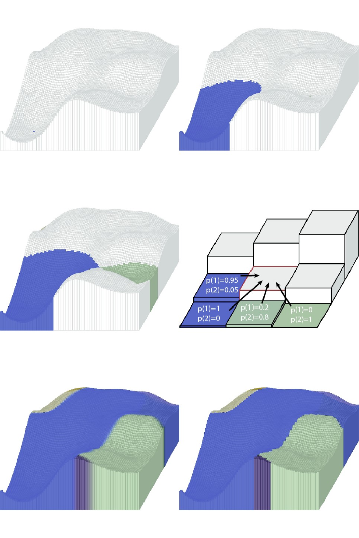
Figure 1: The different steps of the probabilistic algorithm for finding the patches. The height of the histograms is proportional to the density at each pixel of a $2D$ random field. Top-left: the pixel with lowest density is identified and tagged as belonging to the void-patch number $1$ (blue colour) with probability $P(1)=1$. Top-right: the pixels are then considered in ascending order and are tagged according to the tag of their already visited surrounding pixels. This is repeated until the level of the minimum with second lowest density is reached. As this pixel does not have any tagged neighbour, a new void-patch index is added and the pixel is tagged as belonging to it (green colour) with probability $P(2)=1$. Middle-left and middle-right: the process is repeated until one reaches the saddle point with lowest density, located at the border of two patches (middle-left). Above this threshold, a pixel can have several neighbours, each tagged with different patch indexes (middle-right). A list of probabilities associated to the different patch index of the neighbouring pixels is attributed to the current pixel by computing the density difference weighted average of the respective patches probabilities of the surrounding pixels. Bottom-left: repeating the process until all pixels have been visited, one obtains for each pixel a list of possible patches index together with their respective probabilities (hence the blurred borders between patches on the picture). Bottom-right: a clean border between the patches can be found by defining the index of the patch a pixel belongs to as the one with highest probability. It is very straightforward to extend this method to spaces with arbitrary number of dimensions.

The initial idea beyond our patches identification algorithm is that a patch can be defined as the set of field lines (i.e. curves that follow the gradient of a field) that originate from a given minimum (VP) or maximum (PP) of a field. Considering a sampled field, being able to identify the patches thus amounts to being able to decide, for any given pixel $p$, from which extremum all field lines that cross $p$ originate. It is therefore easy to understand that the discrete nature of the sampling rapidly plagues such a task: for each pixel, considering the measured gradient, one has to decide from which, in the fixed number of neighbouring pixels, the field line comes from. Within a $d$-dimensional space, having to select between only $3^{d}$ possibly different direction for field lines is a crude approximation that leads, because of accumulation, to a largely wrong answer for pixels located far away from the extrema.

Although we present the algorithm in the general case here, the reader can refer to figure 1 and its legend for a simpler and more visual explanation of the algorithm in the $2D$ case. More generally, our algorithm involves considering each pixel of a sampled field in the order of their increasing (resp. decreasing) value, depending on whether we want to compute the VPs or PPs and, for each of them, computing the probability that it belongs to a given VP (resp. PP). This probability map is simply computed by scanning the probability distribution of its $3^{d}-1$ neighbours (within a $d$-dimensional space, here $d=2$) and deducing the current pixel patch probability distribution from it. Two cases are possible:

1. none of the neighbours has already been considered (i.e their respective densities are all higher -resp. lower- than that of the current pixel). This means that the pixel is a local minimum (resp. maximum) of the field: a new VP (resp. PP) index is created and the probability that the current pixel belongs to it is set to $100\%$.

2. At least one neighbour has already been considered (i.e its density is lower -resp. higher- than that of the current pixel). The current pixel probability distribution is computed as a gradient weighted average of its lower -resp. higher- density neighbours’ probability distributions.

Once all pixels have been visited, a number $N$ of patches have thus been created and a list of $N$ probabilities $P_{i}^{k}$,$k\in\{1,..,N\}$, has been computed for each pixel, $i$. These probabilities quantify the odds that a given pixel $i$ belongs to a given patch $k$. Figure 2 illustrates the advantages of our probability list scheme compared to the naive approach: without it, the patches borders have a strong tendency to be aligned with the sampling grid and the problem tend to get much worse when considering lower sampling and of course higher dimensions.

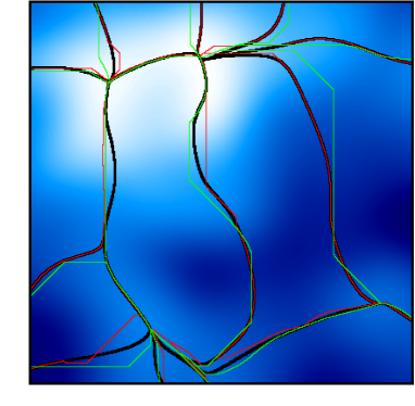
Figure 2: Illustration of the virtue of the probabilistic algorithm. These three curves represent the borders of the void patches obtained with the probabilistic algorithm, by limiting the maximum number of probabilities recorded for each pixel. The black line was derived without any limitation, while for the red one two probabilities were kept and only one for the green one. This last case is equivalent to not using any probability list, as only the values of neighbouring pixels is taken into account. Also note the tendency of the borders to be aligned with the major directions of the sampling grid (namely, the sides and diagonals) when not taking advantage of the probabilistic algorithm.

Figure 3(c) presents the results obtained by applying this algorithm to the $2D$ Gaussian random field of Figure 3(a). On this picture, each patch is assigned a different shade, and the colour of each pixel is the probability weighted average colour of its possible patches. As expected, a majority of pixels seems to belong to a definite void patch with high probability (close to $100\%$). In fact, considering two neighbouring void patches A and B, all the pixels that belong to one of these patches and have a value lower than that of the first kind saddle point(s) on their border (i.e. where the Hessian only has one positive eigenvalue) have a $100\%$ probability of belonging to either A or B. Hence, the probabilities of belonging to different patches only starts mixing above first kind saddle points. This can be seen on the top right zoomed panel of Figure 3(c) where probabilities only start blending mildly for densities above this threshold (the saddle point are represented by the probability “nodes” on the picture). This results in a complex distribution of patch index probabilities in the vicinity of higher density borders (see upper left panel of Figure 3(c)), and thus a higher uncertainty of the location of the void patches border. This uncertainty on the precise patch index is directly linked to the location of the skeleton. In fact, as explained in the next section, the skeleton can also be defined as the set of field lines that do not belong to any patch, or in other terms, where sampled pixels have an equal probability of belonging to several distinct patches.

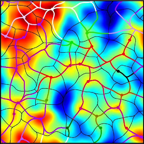
(a) density field

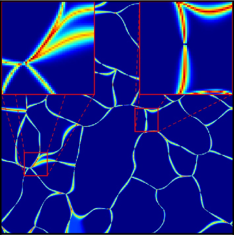
(b) skeleton presence probability

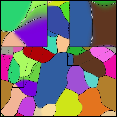
(c) void patches

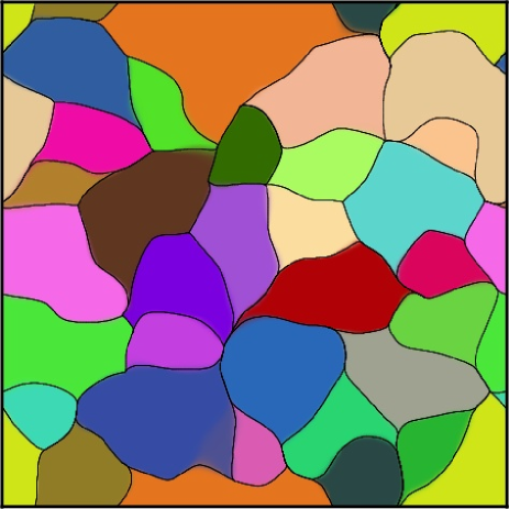
(d) peak patches

Figure 3: Figure 3(a) represents a 2D density field together with its anti-skeleton (black curve) and skeleton (thick coloured curve). The skeleton is coloured according to the value of the index of the underlying void patch, which allows the detection of the saddle points (intersection of the skeleton and void patch borders). A skeleton branch starts from a field maximum (large dots) and goes through one saddle point before reaching another maximum. Figure 3(b) represents, for each pixel, the value of the probability that it belongs to its most probable patch. By definition, the skeleton is the set of points that do not belong to any patch so the lower this value, the more probable the pixel belongs to the skeleton. Figure 3(c) was obtained by attributing a given random colour to each patch index and representing each field with the colour resulting from the probability weighted blend of all patches colours. The zoomed parts show patches borders where the uncertainty on the index of the most probable patch index is maximal. The skeleton is represented in white, together with its smoothed counterpart (black). Figure 3(d) represents the peak patches of the same field.

2.2 The d-dimensional skeleton

As one can easily see, the major strengths of this simple patch extraction algorithm are that it is robust and can be trivially extended to spaces of any dimensions and topology, the only requirement being that one needs to be able to define neighbouring relationships between pixels and measure distances between them. So we now have a robust algorithm for extracting the VP and PP of, in practice, nearly arbitrary scalar fields. In this subsection, we show that it is possible to generalize the definition of the skeleton (Novikov et al., 2006) to spaces of arbitrary dimension and present a simple method to compute the skeleton, as well as critical lines and surfaces, based on our patches extraction algorithm.

2.2.1 Definition

Let us first present important results of the Morse theory without demonstrating them. The more thorough reader can refer to Jost (1995) for a mathematical demonstration.

Let us consider the general case of a sufficiently smooth and non-degenerate $d$-dimensional scalar field $\Phi_{d}({\bf x})$, with ${\bf x}\in M_{d}$ and $M_{d}$ a manifold (i.e $\mathbb{R}^{d}$, the sphere $S^{2}$, …). Following Jost (1995), the field lines of $\Phi_{d}({\bf x})$ fill $M_{d}$ and a VP can be defined as the set of points that can be reached by following the field lines originating from a given minimum of $\Phi_{d}({\bf x})$. The VPs of $\Phi_{d}({\bf x})$ thus segment a set of $d$-dimensional volumes that completely fill $M_{d}$, each of them encompassing exactly one minimum of $\Phi_{d}({\bf x})$. The interface of the VPs, $M_{d-1}$, defines a $(d-1)$-surface (i.e. a surface of dimension $d-1$ embedded in $M_{d}$). It is therefore possible to apply our probabilistic algorithm to $\Phi_{d-1}({\bf x})$, the restriction of $\Phi_{d}({\bf x})$ to $M_{d-1}$, in order to extract the VPs on this interface. For clarity, we will call the VPs of $\Phi_{d-1}({\bf x})$ the first order VPs of $\Phi_{d}({\bf x})$, noted $1$-VPs hereafter. Recursively, the $1$-VPs define $(d-1)$-dimensional volumes that pave $M_{d-1}$, each of them encompassing, by definition of a VP, exactly one minimum of $\Phi_{d-1}({\bf x})$, with coordinates ${\bf m}\in M_{d-1}\subset M_{d}$, and the reasoning can be applied to the whole hierarchy of $\alpha$-VPs, $\alpha\in\{0,..,d-1\}$.

Starting from a $d$-dimensional $C^{2}$ scalar field $\Phi_{d}({\bf x})$, it is thus possible to define a complete hierarchy of sets of $\alpha$-VPs, $\alpha\in\{0,..,d-1\}$. These $\alpha$-VPs are $(d-\alpha)$-dimensional volumes that partition $M_{d-\alpha}$, where $M_{d-\alpha}$ is defined as the $(d-\alpha)$-dimensional interface of the $(d-\alpha+1)$-patches. Each set of $\alpha$-VPs is defined as the set of void patches of $\Phi_{d-\alpha}({\bf x})$, the restriction of $\Phi_{d}({\bf x})$ to $M_{d-\alpha}$. Let us call a critical point, ${\bf x}$, of kind $n$ a critical point with Morse index $\mu\left({\bf x}\right)=n$ (i.e. where the Hessian ${\cal H}\left({\bf x}\right)$ has exactly $n$ positive eigenvalues). Then, $M_{d-\alpha}$ encompasses the whole set of saddle points of kind $n\leq d-\alpha$, of $\Phi_{d}({\bf x})$, the minima of $\Phi_{d-\alpha}({\bf x})$ associated to each $\alpha$-patch being the saddle points of $\Phi_{d}({\bf x})$ of kind $d-\alpha$. The interface $M_{1}$ is thus a curve embedded in $M_{d}$ that links the maxima of $\Phi_{d}({\bf x})$ to its saddle points of kind $1$: the skeleton of $\Phi_{d}({\bf x})$. It is interesting to note that this approach also allows a rigorous definition of the whole set of critical lines similar to the one introduced with the local approximation of the skeleton in Novikov et al. (2006) (see also Sousbie et al. (2008a)), as well as their extension to critical hyper-surfaces of any number of dimensions.

Although we have only addressed the $\alpha$-VPs case so far, the exact same argumentation holds for the whole hierarchy of $\alpha$-PPs, which leads to $M_{d}$ being the skeleton of the voids that links minima to saddle points of kind $d-1$. Moreover, alternating a selection of $n_{v}$ $\alpha_{v}$-VPs and $n_{p}$ $\alpha_{p}$-VPs, $n_{v}+n_{p}=d$, leads to $M_{d}$ being the curve that links saddle points of kind $n_{p}$ to saddle points of kind $n_{p}+1$: a peculiar set of critical lines of the field. One can note that, as rigorously demonstrated in Morse theory (Jost, 1995), critical lines defined in such a way can only link critical points whose Morse index only differ by unity.

2.2.2 Implementation

The representation of the critical lines of a given scalar field as a peculiar limit of a peak or void patches hierarchy certainly has some mathematical appeal. From a practical point of view, although apparently straightforward, its direct numerical implementation can nevertheless be somewhat problematic. Let $G$ be an initial sampling grid and $\bar{G}$ its reciprocal (i.e. $G$ shifted by half the size of the pixels in every direction). Using our patch computation algorithm on a scalar field $\Phi_{d}({\bf x})$ sampled over $G$, we obtain for every pixel, $i$, of $G$ a probability $P_{i}^{k}$ that it belongs to a given patch, $k$. Those sets of probability distributions could be used to define a border between the patches and thus to compute the 1-PPs and 1-VPs. Nevertheless, this is in general not an easy task: one in fact first needs a very precise localization of the 1-PPs and 1-VPs (those living on the (hyper-)surface of the initial VPs or PPs) to be able to compute the following segmentation of the hierarchy (as opposed to a density probability). In order to overcome this issue, we chose first to base our implementation on a subset only of the different patches probabilities and only keep for every pixel the index of its most probable patch. This way, we are able to simply define the borders between patches as the set of pixels of $\bar{G}$ that overlap at least $2$ pixels of $G$ with different most probable patch index. The patches extraction algorithm can then be applied again over that border, restraining pixels examination to the ones that lie on its surface. Identifying pixels of $G$ that overlap at least $2$ pixels of $\bar{G}$ with different most probable patch index, one can thus identify the 2-PP or 2-VP and, repeating this procedure, all orders of the patches hierarchy.

For 2D Gaussian random fields, as pictured on figure 3(d) and 3(c), the skeleton (resp. anti-skeleton) are identical to the VP (resp. PP) borders and the direct implementation of this algorithm leads to a very precise and smooth skeleton. But the implementation in spaces of higher dimensions raises a critical issue with this simplified method, due to the fact that the borders of the $\alpha$-PPs and $\alpha$-VPs are only defined by the index of the pixels they cross: thus they are jagged and considered locally flat (on the scale of one pixel and its direct neighbourhood). Figure 4(a) presents the 1-VPs obtained by applying this algorithm to a 3D Gaussian random field, each colour corresponding to a different 1-VP index. The 1-VPs live on the 2D surface which is the border between the cells formed by the void patches of the field, each of this cell encompassing exactly one minimum of the field. This surface is complex: it can be multiply connected at the interface of more than two different void patches and its curvature is locally significant. Although neighbouring relationships between pixels are easily obtained even where the surface is multiply connected, only a rough approximation of the actual distances along the surface can be computed, as the local curvature is not taken into account. Figure 4(b) shows the corresponding skeleton, computed as the border of the 1-VPs of Figure 4(a). This skeleton is clearly not very well defined, the uncertainty in distance computation leading to errors in the probability propagation algorithm. This bias results in multiple skeleton branches that seem to oscillate and cross each other along the true skeleton location.

In the end, it appears that dropping the full probability distribution and approximating borders between patches is too coarse an approximation. One solution would involve trying to compute the precise location of the $\alpha$-VPs and $\alpha$-PPs using the full set of probabilities, but, as it will be discussed in section 2.3, this raises complex issues. As it is the patches interface computation that seems to be difficult, the alternative we chose to implement involves computing directly the skeleton from the $0-$VPs and $0-$PPs of the field, without having to consider the full hierarchy of $\alpha$-VPs and $\alpha$-VPs. A close examination of Figure 4(a) led us to formulate the conjecture that the $(d\!-\!1)$-VPs or $(d\!-\!1)$-PPs interface corresponds in fact to the subspace of $M_{d-1}$ where the manifold is sufficiently multiply connected (i.e. where the $(d-1)$-surface defined by $M_{d-1}$ folds onto itself). Equivalently, this locus can be defined in $3D$ as the interface of at least $3$ different PPs or VPs (see Figure 4(a)). This is formally demonstrated in Jost (1995). In the general case of $M_{d>3}$, the skeleton should thus be the 1D interface between at least $d$ VPs or PPs of $\Phi_{d}({\bf x})$. Figure 4(c) presents the skeleton obtained using this method on the same Gaussian random field as the one used for Figures 4(a) and 4(b). As expected, as there is no need to recursively compute the full hierarchy of VPs, the resulting skeleton is much more precise and well defined. Moreover, a quick comparison to Figure 4(b) confirms that it is in fact the approximation of the $\alpha$-patches interfaces by individual pixels that plagues the algorithm, each recursive step exponentially increasing the error.

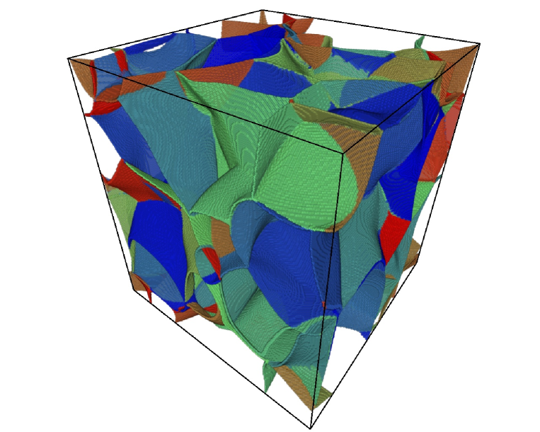
(a) The 1-VPs of a 3D Gaussian random field

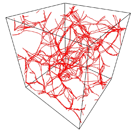
(b) Recursive algorithm

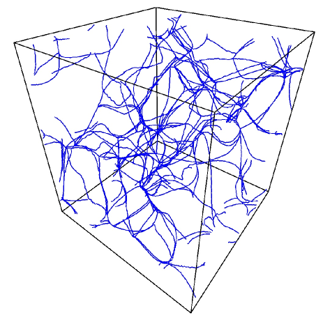
(c) Direct algorithm

Figure 4: Illustration of the computation of the skeleton as the 1D interface of the 1-VPs for a 3D field, $\Phi_{3}({\bf x})$. Figure 4(a) presents the $1$-VPs of $\Phi_{3}({\bf x})$. The 2D surface, $M_{2}$, is computed as the interface of the VPs of $\Phi_{3}({\bf x})$. The 1-VPs are the void patches of the restriction, $\Phi_{2}({\bf x})$, of $\Phi_{3}({\bf x})$ to $M_{2}$. Similarly to picture 3, each colour corresponds to a given 1-VP of $\Phi_{2}({\bf x})$, associated to a given minimum of $\Phi_{2}({\bf x})$ (which is also a saddle point of kind $1$ of $\Phi_{3}({\bf x})$). The rough appearance of $M_{2}$ is due to the fact that it is approximated by the set of pixels of the sampling grid crossed by the interface of the VPs. The skeleton of Figure 4(b) is defined as the interface of the 1-VPs of Figure 4(a): its location is not very precise and it seems to oscillate around its “true” location, mainly because only a locally flat approximation of $M_{2}$ is computed. Conversely, the skeleton of picture 4(c) is computed as the border between at least $3$ PPs of $\Phi_{3}({\bf x})$ or equivalently as the set of points of the surface $M_{2}$ (pictured on Figure 4(a)) which are multiply connected (i.e. where $M_{2}$ folds onto itself). This algorithmically simpler definition leads to a much better defined skeleton.

2.2.3 The skeleton as a set of individual filaments

The concepts introduced above allow the definition and extraction of the skeleton as a fully connected network that continuously link maxima and saddle-points of a scalar field together. It is certainly of interest to try understanding the topological and geometrical properties of this scalar field through the connectivity and hierarchy relationship that it introduces between the critical points. Applied to cosmology, it also allows a formal definition of the concept of individual filaments. Considering matter distribution on large scales in the Universe, a natural definition of a single filament would be a subset of the cosmic web that directly links two halos together. The transposition of such a definition to the skeleton would allow the introduction of useful concepts such as neighbouring relationship between halos in the cosmic web sense. It would also make possible the study of filaments as individual physical objects, similarly to what has been done for years in the literature with the halos and voids.

On Figure 3(a), the skeleton (coloured thick network, where the colour corresponds to the underlying PP index) and anti-skeleton (black network) are superimposed on the density field from which they where extracted. Let us define a filament as a subset of the skeleton continuously linking two maxima together while going through one - and only one - first kind saddle point. These saddle points can be easily extracted as they are located on the skeleton, at the border between the peak (resp. void) patches (i.e where the patch index along the skeleton changes, this definition being valid for any number of dimensions). This way, all the filaments of an N-dimensional distribution can be extracted individually by starting from each maximum of the field, following all the branches of the skeleton, and storing only the paths that cross one saddle point before reaching another maximum. This algorithm thus allows the individual extraction of filaments as well as a continuous wander of the filamentary structure of a distribution, which should be very useful in a wide range of applications in cosmology.

2.3 Sub-pixel resolution and skeleton smoothing

Let us first consider for simplicity a Cartesian sampling grid (even though this sub pixel smoothing does not critically depend on this geometry, see below). The implementation of the procedure of Section 2.2 naturally leads to a skeleton that lives along pixel edges and is thus jagged at the pixels scale. The differentiability of the skeleton is nonetheless a feature which may be critical for a number of its characteristics: its length, curvature, general connectivity … In order to enforce this differentiability, we developed two smoothing methods which we use in practice in turn. The first one is based on a multi-linear interpolation of the patches probability distribution which flows naturally from the original algorithm used to create the skeleton. It provides sub-pixel resolution consistently with the probabilistic framework, thus allowing a precise extraction of the skeleton even when the sampling is low. The other is used to control the level of smoothness away from fixed points (the maxima or the bifurcation points) and can be used to enforce sufficient differentiability.

2.3.1 Multi-linear sub-pixel skeleton

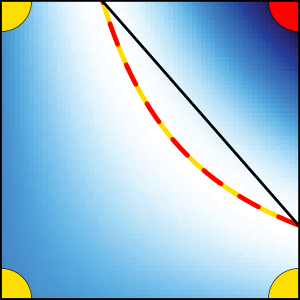
(a) Intersection of $2$ patches

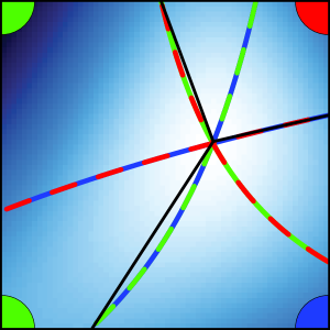
(b) Intersection of $3$ patches

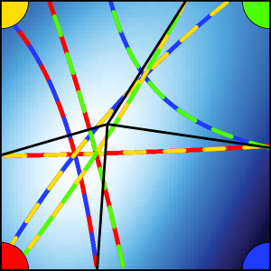
(c) Intersection of $4$ patches

Figure 5: Illustration of the computation of the sub-pixel skeleton in the case of a 2D bi-linearly interpolated pixel located at the border of $2$, $3$ and $4$ different patches. The colour of the pixels vertices represent the index of the dominant patch, while the two-coloured dotted lines are the quadrics, solutions of Equation (6). These lines are the regions where the probabilities corresponding to the patches with similar colours are equal. The underlying blue gradient corresponds to the value of $\tilde{P}({\bf x})$ (Equation (4)), light colours encoding lower value. Finally, the black lines represent our approximation of the smoothed intersection of the skeleton with the pixel.

Let us first find a way to obtain a sub-pixel resolution on the skeleton position based on the patches probability distribution of each pixel. The raw skeleton is made of individual segments located on the edges of the pixels of a Cartesian grid $G$. Each segment is defined by its two end points, and each of them is surrounded by $2^{d}$ pixels with a full list of possible patches index, together with their respective probabilities. Recall that the probabilistic algorithm we use works on individual pixels so the resulting skeleton position, defined as the position of the border between several patches, is computed with a precision of one pixel. This implies that the smoothing procedures may not move the skeleton on more than half the size of a pixel. In other words, if we consider the dual sampling grid, $\bar{G}$, of $G$, the skeleton can be freely moved within the pixels of $\bar{G}$ that its jagged approximation crosses. So it is sufficient to consider individually each of these pixels. Let $\bar{p}$ be one of these pixels. We then know for each of its vertices, $p_{i}$ with $i\in{1..2^{d}}$, the probability distribution of the different VPs, $P_{i}^{k}$, where k is the index of a VP. In order to obtain sub-pixel resolution, these probabilities can be interpolated within $\bar{p}$.

For simplicity, we will only use a multi-linear interpolation and define $P^{k}({\bf x})$, the probability distribution of patch $k$, interpolated at point ${\bf x}=(x_{1},..,x_{d})\in[0,1]^{d}$ within $\bar{p}$ as:

$$P^{k}({\bf x})=\sum_{i=1}^{2^{d}}P_{i}^{k}\prod_{j=1}^{d}\epsilon_{j}^{i}(x_{j}),$$ (2)

where $\epsilon_{j}^{i}(x)=x$ if the $j^{th}$ coordinate of $p_{i}$ within $\bar{p}$ is $1$ and $\epsilon_{j}^{i}(x)=(1-x)$ if it is $0$. Ideally, the skeleton should not belong to any VP, so it should be located where all the non null values of $P^{k}({\bf x})$ are equal. Let us define the arithmetic mean of the probability (over the VPs with index $k$) over the pixel

$$\left<P({\bf x})\right>=1/N\sum_{k}^{N}P^{k}({\bf x}),$$ (3)

and its root mean square,

$$\tilde{P}({\bf x})=\sqrt{\sum_{k}^{N}\left(P^{k}({\bf x})-\left<P({\bf x})\right>\right)^{2}},$$ (4)

where the sum is over all the $N$ subscripts $k$ such that there exist a pixel $p_{i}$ where $\forall l\neq k,P_{i}^{k}>P_{i}^{l}$. Clearly, all patches with dominating probabilities $P^{k}({\bf x})$ in $\bar{p}$ are equal when

$$\tilde{P}({\bf x})=0.$$ (5)

Equation (5) is of fourth order and is thus difficult to solve in general.

2.3.2 Approximate quadrics sub-pixel smoothing

Insights into the solution of Equation (5) can be found while considering the intersection sets of points where pairs of probabilities are equal instead of equating them all at the same time. These sets are solution of the set of equations

$$P^{k}({\bf x})=P^{k\prime}({\bf x}),\quad k\neq k\prime$$ (6)

where $k$ and $k\prime$ are subscripts of the patches that dominate on at least one vertex of $\bar{p}$.

For clarity, let us consider the $d=2$ case first. With a proper indexing of the four pixels $p_{i}$,

$$P^{k}({\bf x}) = P_{1}^{k}(1-x_{1})(1-x_{2})+P_{2}^{k}(x_{1})(1-x_{2})$$ (7)

$$+P_{3}^{k}(1-x_{1})(x_{2})+P_{4}^{k}(x_{1})(x_{2}),$$

Equation (6) writes in this case:

$$A\,x_{1}x_{2}+B\,x_{1}+C\,x_{2}+D=0\,,$$ (8)

where $A$, $B$, $C$ and $D$ only depend on the values of $P_{i}^{k}$. Equation (8) is quadratic and its solutions are well known curves of dimension $d-1=1$ called quadrics. Figure 5 illustrates solutions of Equation (8) when $\bar{p}$ is located at the intersection of $N_{p}=2$, $N_{p}=3$ or $N_{p}=4$ different VPs. In the most frequent configuration where $\bar{p}$ is at the intersection of $2$ VPs, Equation (8) directly gives the first order approximation of the intersection of the skeleton and $\bar{p}$, and we may approximate it by a straight segment. Finding the end points of this segment is easily achieved by computing the location of equal probability along the two sides of $\bar{p}$ that link vertices with different patches (Figure 5(a)). The $N_{p}=3$ configuration is rarer, and concerns only the maxima of the field as well as all bifurcation points of the skeleton. In this case, we know that three different branches of the skeleton merge within the pixel, at a point where all probabilities are equal. So, we may set the bifurcation point as the locus where all the $C_{2}^{3}=3$ quadrics of Equation (6) intersect (note that the three of them always intersect in a single point as $P^{1}({\bf x})=P^{2}({\bf x})$ and $P^{1}({\bf x})=P^{3}({\bf x})$ implies $P^{2}({\bf x})=P^{3}({\bf x})$). The three branches of the skeleton in $\bar{p}$ are thus obtained by linking the bifurcation point to the iso-probability along the three sides of $\bar{p}$ that link vertices associated to different patches (Figure 5(b)). Finally, the $N_{p}=4$ configuration is very rare and also more problematic. As previously, we know that there exist a bifurcation point within $\bar{p}$, but this time with $4$ different skeleton branches. Since there are now $C_{2}^{3}=6$ different Equations (6), and given that the solution of each of them is a 1D quadric, this system is clearly over constrained to find the precise location of the bifurcation point. A solution may well be to use a higher order interpolation, allowing more complex curves than quadrics for equal probabilities regions, or to try solving directly Equation (5). As this case is clearly rare, it would also be possible to approximate the bifurcation point as the barycenter of the three points of intersection of the subsets of Equations (6) taken in pairs. Again, the smoothed skeleton would therefore be derived by linking the bifurcation point to the four iso-probability points along the four sides of $\bar{p}$ (Figure 5(c)).

2.3.3 Actual recursive implementation

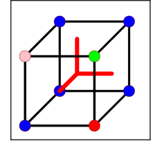
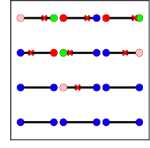
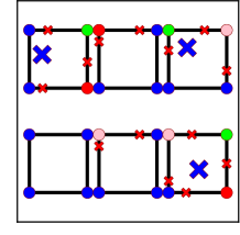
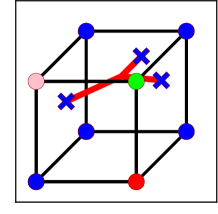
Figure 6: Illustration of different steps of the recursive algorithm used to obtain sub-pixel resolution for the skeleton, in 3D. The colour of the balls represent the index of the patch with maximal probability while the intersection of the skeleton and the cell is displayed in red. The algorithm consists in recursively considering the $n$-dimensional faces of the sampling unit volume (here an hypercube). For a 3D Cartesian sampling grid, one starts equating dominant probabilities on the vertices of edges, then faces and finally the cube.

Having discussed the underlying geometry of the sub-pixel multi linear interpolation, let us now turn to our actual sub-pixel smoothing algorithm. Indeed, in $d$-dimensions, Equation (6) is of order $d$ and is linear in each of the $d$ space coordinates $x_{i}$. Its solutions are thus $d-1$ dimensional quadrics whose intersections, as in $2D$, can be used to recover the skeleton position down to a sub-pixel precision. Finding intersections of quadrics in general remains nonetheless a highly difficult (or even untractable!) problem and even state-of-the-art solvers can only achieve such a performance for $d=3$ at most. To circumvent this difficulty, we thus opted in practice for a different solution that consists in a recursive numerical minimization of the value of $\tilde{P}({\bf x})$ over the hierarchy of n-cubes (i.e hypercubes of dimension $n$), $n\in\{1,..,d\}$, that are the faces of each cell of the sampling grid. The trick is to always reduce the problem to a 1D minimization of a polynomial of order $d$ (see appendix A). Figure 6 illustrates the full process in 3D. Let us consider the grid cell of Figure 6, located at the interface of $4$ different patches. The skeleton extraction algorithm produces the jagged skeleton represented in red. In order to improve its resolution, we first consider each of the $12$ edges individually (see Figure 6) and determine for each of them the point of equal probability for the two patches that dominate at the end points of segment. Of course this point only exists if different patches dominate at the end points of a segment and we thus obtain at most $12$ new points ($7$ in this instance, represented by the red crosses). The edges of a cube can be considered as its “one dimensional faces” or $1$-faces. The following step consists in examining the configuration of its $2$-faces, usually called faces for a 3D cube. Figure 6 illustrates the configuration of these $6$ faces together with the iso-probability points computed over their edges. We know that at least $3$ different patches have to dominate on at least one of the $4$ vertices of each face for a skeleton branch to enter the cell through this face. Using the minimization algorithm presented in Appendix A and the iso-probability points on the edges, it is thus possible to compute, over these faces, the location of the minimum of $\tilde{P}({\bf x})$ (represented as blue crosses on Figure 6). Finally, considering the $3$-face of the cell (i.e. the cube itself), one can determine the point of minimal value of $\tilde{P}({\bf x})$ over the cube, which is the point where the skeleton branches connect (see figure 6).

The generalization of this algorithm is relatively straightforward. Let us again consider a cell that is a hypercube of dimension $d$. We know that the skeleton intersects this cell if at least $d$ of its vertices have different maximal probability patches index. In that case, the sub-pixel resolved skeleton can be recovered by considering all the $n$-faces of the hypercube, $n\in\{1,..,d-1\}$, in ascending order of their dimension $n$. When considering a $p$-face, we minimize the value of $\tilde{P}({\bf x})$ in order to obtain the point where its vertices respective patches have equal probability, using the points obtained from the $(p-1)$-faces. This point only exist for a $p$-face if at least $(p+1)$ vertices most probably belong to different patches. In the end, one thus obtains a number of points from the $(d-1)$-faces that are the points where the skeleton enters the cell and one point for the $d$-face (i.e. the cell itself), which gives the location where different branches of the skeleton connect. Figure 7 illustrates the result of applying this algorithm in the $2D$ case.

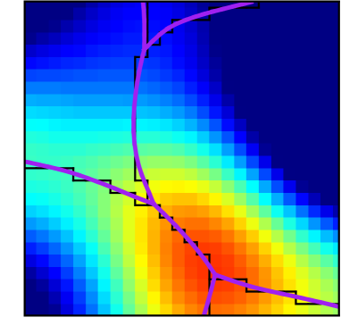
Figure 7: Illustration of the skeleton with a sub-pixel resolution in 2D. The background pixels colour represent the sampled density field while the black skeleton was obtained using our probabilistic algorithm. The purple skeleton is the post-treated version of the black one. Note how any sampling grid influence disappeared, especially in the originally vertical segment located in the upper-left corner of the image.

2.3.4 Artifacts correction and differentiability

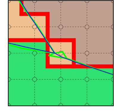
Figure 8: A failure of the skeleton sub-pixel algorithm due to the lack of sampling resolution. The dotted grid represents the reciprocal sampling grid, $\bar{G}$, while the pixels colour represents their dominating patches and the initial raw skeleton is represented in red. The green skeleton is the result of applying the sub-pixel resolution algorithm while the blue one was obtained from the green one, after removing one pixel sized loops and smoothing.

Though the method presented above to obtain sub-pixel resolution works most of the time, there nonetheless exist situations where it can fail due to sampling effects. Figure 8 illustrates such a situation, which can sometimes occur when the sampling grid pixel size is not totally negligible compared to the average extension of the patches. When the thickness of a peak or void patch is smaller than a pixel size, it can in fact lead to mistakingly isolated subregions of size one pixel, implying the creation of spurious loops in the skeleton (in red). This phenomenon, although rare, occurs in spaces of arbitrary dimension and triggers artifacts when applying our sub-pixel resolution algorithm. The green skeleton on Figure 8 presents such an example of a spurious skeleton loop.

In order to fix these anomalous segments, we chose to post-treat the skeletons by opening-up all one-pixel sized loops and smooth the resulting skeleton to enforce a desired level of differentiability in the skeleton trajectory (see the blue skeleton of Figure 8). The smoothing method that we use presents the advantage of being quite robust, and involve fixing some specific points of the skeleton, and averaging the position of each non-fixed segments end points with the position of its closest neighbouring end points a number of times. Let $x^{i}_{j}$ be the $j^{th}$ coordinates of the $i^{th}$ sampled skeleton location (among $N$) between two fixed points. Before smoothing, all $x^{i}_{j}$ are located on the edges of $G$ and we can define their smoothed counterparts as $y^{i}_{j}$, computed as:

$$y^{i}_{k}=A^{ij}x^{j}_{k},$$ (9)

with

$$A^{ij}=\left\{\begin{array}[]{l}3/4\quad{\rm if}\quad i=j=0\quad{\rm or}\quad i=j=N,\\ 1/2\quad{\rm if}\quad i=j,\\ 1/4\quad{\rm if}\quad i=j+1\quad{\rm or}\quad i=j-1,\\ 0\quad{\rm elsewhere,}\\ \end{array}\right.$$ (10)

where Equation (9) is applied $s$ times in order to smooth over $s$ segments. Basically, Equation (9) is used to compute smoothed coordinates $y^{i}_{j}$ as a weighted average of the original coordinates $x^{i}_{j}$ together with the coordinates of its $2$ direct neighbours, $x^{i-1}_{j}$ and $x^{i+1}_{j}$. Applying this scheme $s$ times thus produces the final smoothed coordinates $y^{i}_{j}$ to be a weighted average of $x^{i}_{j}$ and its $s$ closest neighbours along the skeleton.

This smoothing technique introduces two parameters of importance: the skeleton smoothing length $s$, and the type of fixed points. In order to determine the optimal value of $s$, it is possible to minimize the reduced $\chi^{2}$ corresponding to the discrepancy between $y^{i}_{j}$ and $x^{i}_{j}$ supplemented by a penalty corresponding to the total length of the skeleton (over-smoothing will increases the discrepancy, under-smoothing will increase the total length). In practice, though, as a post treatment to an already smooth skeleton (using the sub pixel probabilities), this choice is not critical.

The choice of the skeleton points that should be fixed before smoothing depends of the planned application; in practice, we implemented two possibilities: (i) fixing the field extrema, or (ii) the bifurcation points of the skeleton (i.e the points of the skeleton where two filaments merge into one). Figure 9 illustrates the influence of this choice on the shape of the smoothed skeleton. By fixing the extrema of the field, one ensures that the skeleton subsets that link these extrema are treated independently: this is the solution used to study the properties of individual filaments in the dark matter distribution on cosmological scales. One should note that, in this case, the parts of the skeleton that belong to several individual filaments are duplicated (see the red skeleton on Figure 9), affecting global properties of the skeleton such as its total skeleton length. In contrast, fixing bifurcation points enforces the smoothing of the skeleton while conserving its global properties.

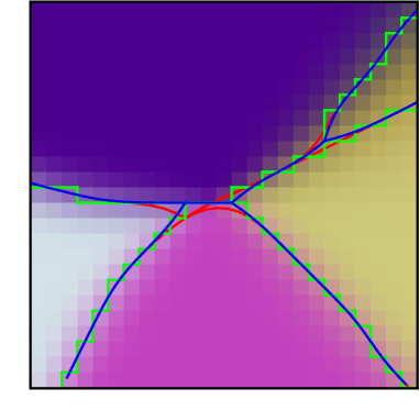
Figure 9: Influence of the choice of fixed points on the shape of the smoothed skeleton. The original skeleton is represented in green, while the red and blue skeletons are smoothed $s=6$ times, while fixing the field maxima and the bifurcation (i.e multiply connected) points respectively. In both cases, the smoothed versions always stay within half the size of a pixel distance from the original non-smoothed skeleton. On this illustration, the smoothed skeleton was computed directly from its raw jagged version to emphasize the effect of the choice of different fixed points. This discrepancy between the two options is considerably weakened if the skeleton is previously post-treated. The background colour corresponds to the weighted probability each pixel has to belong to a definite patch.

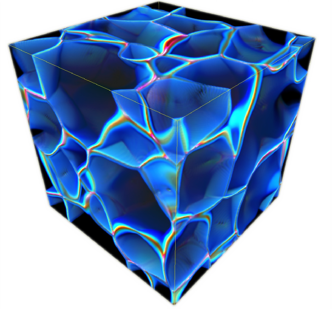
Figure 10: the 3D peakpatch colour coded probability function: warm colours correspond to equiprobability regions, dark colours to regions where one probability dominates (see also Figure 3(b)). This supplementary map complements the peakpatch map in the present algorithm and allow for a precise sub pixel segmentation and skeleton extraction. Note the extended equiprobability sheets corresponding to places where the exact position of the filament will be more uncertain.

2.4 Summary

Let us finally recap the main steps involved in the extraction of the fully connected skeleton in a $d$-dimensional space.

1. The density field is sampled and smoothed in order to ensure sufficient differentiability. A smoothing scale of at least $5$ pixels is recommended when using a Cartesian grid.

2. All pixels are considered in the order of their ascending (or descending) density. Depending on their neighbours, they are labelled as minima (or maxima), or assigned a list of probability to belong to a given VP (or PP) following the algorithm of section 2.1.

3. Considering only the patch index with highest probability for each pixel, skeleton segments are created on pixel edges when at least $d$ surrounding pixels among $2^{d}$ have a different most probable patch index.

4. Calling a vertex connected to more than two segments a node of the skeleton and considering each node, the sets of connected segments that link them to other nodes are recorded in order to later recover the information on the skeleton connectivity (and allow a continuous wander along the fully connected skeleton).

5. The sub-pixel smoothing procedure of Sec. 2.3.3 is implemented. All the vertices of the skeleton segments are considered one by one together with the value of the probability distribution in the center of the surrounding pixels. According to the sub-pixel algorithm, the extremities are moved in order to obtain a differentiable skeleton.

6. Configurations that are identified as problematic are corrected for following the method described in section 2.3.4, and the resulting skeleton is smoothed over a few pixels (usually $d$ of them) while fixing either bifurcation points or maxima/minima.

7. Eventually, individual filaments can be extracted (and tagged) following the method of section 2.2.3.

Figures 11 and 12 show a 3D skeleton computed from a simulated density field at $z=0$, sampled over only $128^{3}$ pixels.

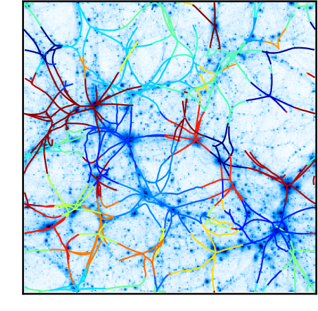
Figure 11: The 2D projection of a 3D skeleton computed on a simulation of the cosmological density density field in a $50h^{-1}$ Mpc box with gadget-2. This $20h^{-1}$ Mpc thick section of skeleton was computed from a $128^{3}$ pixels sampling grid smoothed over $5$ pixels ($\approx 2h^{-1}$ Mpc). The skeleton colour represents the index of the peak patch. Note that the 2D projection of a 3D skeleton differs from the skeleton of the 2D projection, hence the discrepancy between the skeleton and apparent filaments.

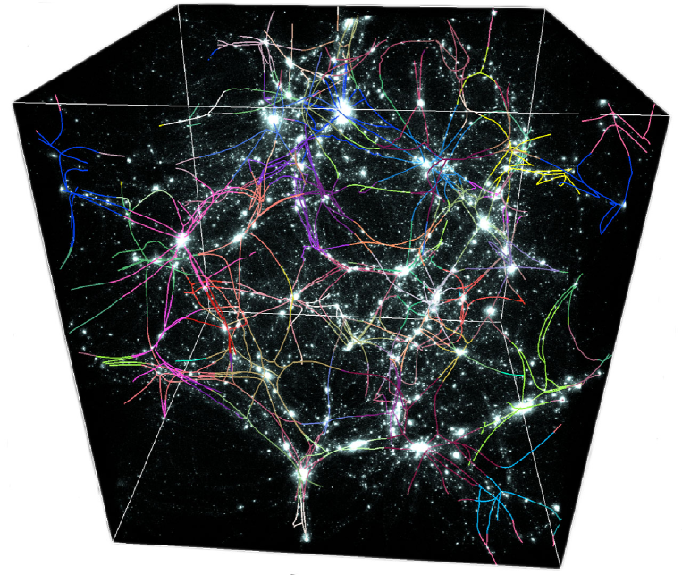
Figure 12: The 3D skeleton of the simulation of the cosmological density density field in a $50h^{-1}$ Mpc box with gadget-2 (see also Figure 11). This skeleton was computed from a $128^{3}$ pixels sampling grid smoothed over $5$ pixels ($\approx 2h^{-1}$ Mpc). The skeleton colour represents the index of the peak patch (which provide by construction the natural segmentation of filaments attached to the different clusters.). Movies of 3D skeletons can be downloaded at http://www2.iap.fr/users/sousbie/

Note that in this paper, we did not address the issue of shot noise that has for long been known to be a problem for most segmentation algorithms, and in particular for Watershed techniques (see e.g. Roerdink (1995) for a review on the subject). In fact, shot noise often leads to over segmentation, and numerous complex techniques have been developed to try and compensate for it. Instead, we chose here to follow the approach used in Novikov et al. (2006), Sousbie et al. (2008a) and Sousbie et al. (2008b), that involve simply filtering the sampled fields using a Gaussian kernel on large enough scales (in terms of number of sampled pixels) so that it is possible to consider that the sampled field is a smooth enough representation of the underlying field. A clear disadvantage of this method is that it introduces a particular smoothing scale and thus adds one parameter (the smoothing scale) to take into account when considering sets of critical lines an surfaces computed on a field. A short study of the robustness of the skeleton extraction in the case of a smoothed scalar field is presented in appendix C. Improvements over this shortcoming are postponed to further investigations.

Regarding performance, the computing time and memory consumption for the extraction of the skeleton mainly depends on three parameters: the number of pixels $N_{p}$, the smoothing length $L$ in units of pixel size and the number of dimensions $N_{d}$. Most of the computational power is spent during the first step of the process: the propagation of the probabilities to compute the patches. For a constant value of $L$ and $N_{d}$, the algorithm speed is linear in $N_{p}$, and so is the memory consumption. A smaller value of $L$ implies more smaller patches, which therefore have proportionally more borders with each other thus increasing the number of different probabilities to propagate. Indeed, for very small values of $L$, memory consumption is largely increased as well as the computational time; it seems reasonable to keep $L$ above a minimal threshold of $L\geq 5$ pixels (which in any case is also necessary to ensure sufficient differentiability of the sampled field). Finally, the value of $N_{d}$ is most critical to memory consumption and speed, not only because $N_{p}$ should increase with $N_{d}$ to keep a constant sampling resolution, but also because the number of neighbours for each pixels scales as $3^{N_{d}}$ for a Cartesian grid. The computational time and the memory consumption follows, as the number of different probabilities to keep track of is also much increased (each pixels having many more neighbours, the ratio of patches interface surface to their volume increases and so does the number of different probabilities to propagate, on larger distances). For the different skeletons presented in this paper, to give and order of magnitude, for a single modern CPU, $2D$ skeletons of $1024^{2}$ pixels smoothed over $l\approx 10$ pixels are computed in a matter of few seconds and the memory needed is of order $\approx 10$ MBytes. Computing a $3D$ skeleton on a $128^{3}$ pixels grid with $L\approx 6$ takes approximately $1$ minute and a hundred of MegaBytes of memory, while for a $512^{3}$ grid, it takes about an hour and around $14$ GBytes of memory are used. While $4D$ skeletons are still tractable at a descent resolution , higher dimensionality seems difficult to reach with present facilities without implementing a fully parallel version of the code.

3 An application: validating the Zel’dovich mapping

The scope of application of the algorithm presented in Sec. 2 is vast (see Sec. 4 for a discussion). Here we shall focus on a simple example which makes use of one of the clear virtues of the above implementation: it allows us to identify as physical objects the filaments present in the matter distribution on cosmological scales, and see how these objects evolve with time.

Specifically, we intend to show, using the skeleton as a diagnostic tool, that a relatively simple but powerful model, namely the truncated Zel’dovich approximation mapping (Zel’Dovich, 1970), can capture the main features of the cosmic evolution of the web. Indeed predicting the evolution of matter distribution from the point of view of the topology and the geometry of the cosmic web has been a recurrent issue in cosmology (e.g. Bond & Myers (1996)) and is becoming critical as the geometry of the cosmic environment is now believed to play a key role in shaping galaxies (see, e.g. Ocvirk et al. (2008)).

Being able to carry such an extrapolation from the initial condition to the present day distribution of filaments should lead to a simplified and broader understanding of large scale structures in the Universe, in the same way the concept of clusters as important physical objects gave birth to the hierarchical model of structure formation. The fully connected skeleton encompasses both the geometry and the topology of the cosmic web: it is therefore the ideal tool to validate this mapping between the initial condition and the present day distribution of filaments. Understanding and partially correcting for the distorsion induced by the proper motions of the structures is also of prime importance when dealing with observationnal data sets (see e.g. Pichon et al. (2001)).

The principle of the Zel’dovich approximation (ZA hereafter) is to make a first order approximation, in Lagrangian coordinates, of the motion of the collisionless dark matter (DM) particles. The motion of these particles from the initial mass distribution in Lagrangian coordinates ${\bf q}$ to their Eulerian coordinates ${{\bf x}}$ can therefore be described as:

$${\bf x}\left(z,t\right)={\bf q}+D\left(z\right)/D\left(z_{i}\right){\bf\Psi}_{i}\left({\bf q}\right),$$ (11)

where $z$ is the redshift, $D\left(z\right)$ the growth factor, and ${\bf\Psi}_{i}\left({\bf q}\right)$ the displacement field, computed in the initial matter distribution as:

$${\bf\Psi}_{i}\left({\bf q}\right)=\frac{-2D}{3{H_{\rm in}}^{2}\Omega_{\rm in}}{\bf\nabla_{{\bf q}}}\phi$$ (12)

where $H$ is the Hubble constant, $\Omega$ the quantity of energy in the Universe, $\phi$ the gravitational potential and the subscript “in” stands for initial conditions. The truncated Zel’dovich approximation simply consists in filtering short scale modes of the initial power spectrum before computing the displacement field in order to prevent shell crossing effects. It has been shown to improve the precision of the approximation (Coles et al., 1993). As we are mainly interested in the large scale behavior of the cosmic web, the smoothing scale, $L=L_{\rm NL}\approx 3.94$ Mpc, that we use hereafter to compute ${\bf\Psi}_{i}$ roughly corresponds to the scale of non linearity at $z=0$, as the so called truncated Zel’dovich approximation has been shown to work best above this scale (Kofman et al., 1992). It was computed as the scale at which, in the simulation, the smoothed density field, $\rho(L)$, is such that $\sigma^{2}(L_{\rm NL})=\left<(\rho(L_{\rm NL})-\bar{\rho}(L_{\rm NL}))^{2}\right>=1$ at $z=0$.

3.1 Simulation and skeletons

The numerical simulation that we use in this section was computed with the publicly available N-body code GADGET2 (Springel, 2005). It corresponds to a dark matter only cosmological simulation of $512^{3}$ particles within a $250h^{-1}$ Mpc cubic box, considering a $\Lambda$CDM concordant model ($H_{0}=70$, $\Omega_{b}=0.05$, $\sigma_{8}=0.92$, $\Omega_{\Lambda}=0.7$ & $\Omega_{0}=0.3$). In order to study the evolution of the cosmic web, a set of reference skeletons, ${\cal S}_{\rm simu}(z,L)$, were computed from different snapshots, at redshift $z=\{{0,0.15,0.3,0.5,0.66,1.15,3,5,10\}}$, where $z=z_{i}=10$ corresponds to the redshift of the initial conditions of the simulation. These skeletons were computed on density fields generated by sampling the particle distribution of the respective snapshots on a $512^{3}$ grid and after smoothing with a Gaussian kernel of size $L=L_{\rm NL}\approx 3.94$. In order to understand if the truncated Zel’dovich approximation is able to capture the essential features of cosmic web, these skeleton are compared to different sets of skeletons, generated using the truncated Zel’dovich approximation in different ways:

• ${\cal S}_{\rm ZA}(z,L_{\rm NL})$: This set of skeletons is generated by applying the Zel’dovich approximation to the DM particles of the simulation in the initial conditions. The displacement field is computed after smoothing over the scale $L_{\rm NL}$ and the resulting distribution is sampled and smoothed over the same scale to generate the skeletons.
  

• ${\cal S}_{\rm SZA}(z,L_{\rm NL})$: these skeletons are generated by applying the Zel’dovich approximation directly to the skeleton of the initial conditions. The initial condition simulation ($z_{i}=10$) is sampled and smoothed over the scale $L_{\rm NL}$ to compute its skeleton. The displacement field is computed on the same field, but smoothed over a scale $L_{\rm l}\approx 8.81$ Mpc (such that $\sigma^{2}(L_{\rm l})=0.5$ at $z=0$) and the Zel’dovich approximation is applied to each segment of the initial condition skeleton. We use a larger truncation scale for the Zel’dovich approximation here in order to prevent shell crossing, which can be tolerated when applied to particles but would result in a very fuzzy displaced skeleton.
  

• ${\cal S}_{\rm ZAL}(z,L_{\rm NL})$: same as ${\cal S}_{\rm ZA}(z,L_{\rm NL})$, but with a displacement field smoothed over the scale $L_{\rm l}$, in order to check the influence of this choice on ${\cal S}_{\rm SZA}(z,L_{\rm NL})$.
  

• ${\cal S}_{\rm ZA}(z,L_{\rm cor})$: same as ${\cal S}_{\rm ZA}(z,L_{\rm NL})$, but the sampled field is smoothed on a scale $L_{\rm cor}$ instead of $L_{\rm NL}$ to take into account that the Zel’dovich approximation introduces an artificial additional smoothing scale (see below).

3.2 Skeleton length

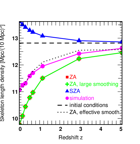
Figure 13: Measured length of the skeleton per unit volume as a function of redshift $z$. The length density was measured on the simulation (purple discs), its truncated Zel’dovich approximation whose displacement field was computed using a smoothing length $L\approx 3.94$ such that $\sigma(L,z=0)=1$ (red squares), or $L_{l}\approx 8.81$ such that $\sigma(L,z=0)=0.5$ (green crosses), and finally using the displacement field of the Zel’dovich approximation at scale $L_{l}$, applied directly to the skeleton of the initial condition, at $z=10$ (blue triangles). The black dashed line stands for the length of the skeleton in the initial conditions (at $z=10$), while the dotted line represents the length measured using the Zel’dovich approximation on the initial condition while taking into account the effective smoothing introduced by using the Zel’dovich approximation. This recipe yields the best match with the simulation. Except for this last case, the skeletons where computed after smoothing the density field with a Gaussian kernel of width $L$.

There exist many different ways to compare one dimensional sets of lines within a $3D$ space, but one of the simplest certainly involves comparing their lengths. Figure 13 presents the measured length per unit volume of the different sets of skeletons (described above) as a function of redshift. Let us first consider the length of ${\cal S}_{\rm simu}(z,L_{\rm NL})$ (purple curve with discs symbols). It was shown in Sousbie et al. (2008a) and Sousbie et al. (2008b) that, whereas for scale invariant fields such as the initial conditions of the simulation, the length of the skeleton is expected to grow as $L^{-2}$ ($L$ being the smoothing length), it grows in fact as $\approx L^{-1.75}$ around $z=0$ for $\Lambda$CDM simulation. Note that the fact that the length of ${\cal S}_{\rm simu}(z,L_{\rm NL})$ decreases with time seems consistent with the expected evolution of matter distribution in the case a cosmological constant, where the expansion accelerates around $z\approx 1$. In that case, matter in fact tends to form separate distant heavy halos: more numerous small filaments on smaller scales shrink and melt into each other as dark matter halos merge, while larger scale filaments tend to stretch: the net result is a total length decrease.

This process seems to be well captured by the Zel’dovich approximation as the length of ${\cal S}_{\rm ZA}(z,L_{\rm NL})$ (red curve, square markers) exhibits the same time evolution as the length of ${\cal S}_{\rm simu}(z,L)$. The discrepancy between the measured length in the simulation and with Zel’dovich’s approximation is nonetheless of the order of $\approx 10\%$ at $z=0$. This disagreement should be explained in part by the fact that the Zel’dovich approximation uses a displacement field computed from a smoothed version of the initial condition density field, thus introducing an additional smoothing that one should take into account when computing ${\cal S}_{\rm ZA}$.

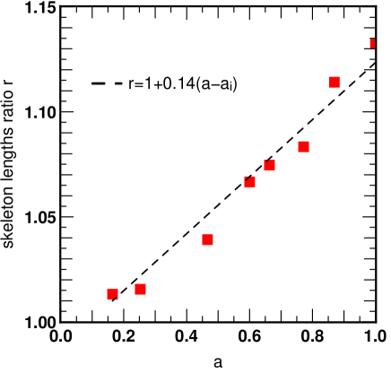
Figure 14: Ratio of the length of the skeleton measured in the simulation to the length of the skeleton of the Zel’dovich approximation as a function of time, a. The dashed line represents the best fit of the data (red squares).

The measure of the ratio, $r$, of the length of ${\cal S}_{\rm simu}(z,L_{\rm NL})$ to the length of ${\cal S}_{\rm ZA}(z,L_{\rm NL})$ as a function of time, $a$, is displayed on Figure 14. It appears that $r$ is approximately a linear function of time, $a$, and can thus be fitted as

$$r=1.00+0.14\left(a-a_{i}\right),$$ (13)

where $a_{i}=1/\left(1+z_{i}\right)\approx 0.09$ is the time of the initial conditions from which the Zel’dovich approximation was computed. Moreover, the fact that the value of $r$ is relatively close to unity confirms that the artificial smoothing introduced by the Zel’dovich approximation is small; we chose to model it as a convolution with a Gaussian kernel of size $L_{\rm ZA}$. The effective Gaussian smoothing used on Zel’dovich’s approximation has scale $L_{\rm eff}$ and is thus the result of the composition of two Gaussian smoothing of scale $L_{\rm ZA}$ and $L_{\rm NL}$:

$$L_{\rm eff}=\sqrt{{L_{\rm ZA}}^{2}+{L_{\rm NL}}^{2}}.$$ (14)

Using equations (13) and (14), and the fact that the skeleton length grows with smoothing scale as $\approx L^{-1.75}$ (Sousbie et al., 2008b), the value of $L_{\rm ZA}$ one should chose to get the best match with $\Lambda$CDM simulations is thus

$$L_{\rm ZA}\approx L_{\rm NL}\left(\frac{2\cdot 0.14}{1.75}\left(a-a_{i}\right)\right)^{1/2}=0.4L_{\rm NL}\sqrt{a-a_{i}}.$$ (15)

In order to compute a skeleton that is comparable to ${\cal S}_{\rm simu}(z,L_{\rm NL})$, one should therefore smooth the distribution obtained using the Zel’dovich approximation on a scale $L_{\rm cor}$ such that

$$L_{\rm cor}=\sqrt{{L_{\rm NL}}^{2}-{L_{\rm ZA}}^{2}}=L_{\rm NL}\sqrt{1.00-0.16\left(a-a_{i}\right)}.$$ (16)

On Figure 13, the dotted black curve represents the measure of the length of ${\cal S}_{\rm ZA}(z,L_{\rm cor})$, when the effective smoothing introduced by the Zel’dovich approximation is taken into account. The agreement with the measurements in the simulation is significantly improved compared to the naive approach; this suggest that the Zel’dovich approximation can be used to predict the shape of the evolved cosmic web from the initial conditions distribution only.

Of course, the length is only a global characteristic of the skeleton and it certainly does not fully constraint its shape. Higher order estimators that can compare the relative position and shapes of skeletons are needed to quantify how good an approximation the skeleton obtained by Zel’dovich’s approximation is.

Before doing so, let us consider an alternative form of the Zel’dovich approximation, where, instead of displacing the particles from the initial conditions of the simulation to derive the evolved density field, we directly use the displacement field to evolve the skeleton of the initial conditions. This method will be called here the skeleton Zel’dovich approximation (SZA hereafter), and the resulting skeleton ${\cal S}_{\rm SZA}$. Studying the properties of ${\cal S}_{\rm SZA}$ is interesting as it should make it possible to distinguish between two different processes that affect the properties of the cosmic web: the simple deformation of the initial cosmic web on the one hand and the creation or annihilation of filaments on the other hand. Indeed, ${\cal S}_{\rm SZA}$ reflects only the modification of the skeleton due to its deformation while ${\cal S}_{\rm ZA}$ also takes into account the merging and annihilation of filaments. Note nonetheless that by definition, the locus of the skeleton for the SZA is biased toward higher density regions; in these regions, non-linear effects inducing shell-crossings in the Zel’dovich approximation are more likely. To be conservative, we thus use a larger smoothing length than $L_{\rm NL}$ to compute the displacement field. This smoothing length, $L_{\rm l}\approx 8.81h^{-1}$ Mpc, was chosen such that $\sigma(L_{\rm l},z=0)=0.5$; the green curve (cross markers) of Figure 13 shows that using $L_{\rm l}$ or $L_{\rm NL}$ does not make any difference regarding the length of the skeleton. On this figure, the blue curve (triangle markers) depicts the evolution of the length of ${\cal S}_{\rm SZA}(z,L_{\rm NL})$: its behavior is clearly opposite to the ${\cal S}_{\rm ZA}$ case, as the length rises with time. Although surprising at first sight, this result only confirms our previous interpretation of the evolution of the cosmic web. In fact, if the SZA can nicely capture the large scale evolution of long filaments, the smaller ones cannot melt into each other, which induces several small scale filaments to be located at the same loci, where only one piece of filaments should have been measured. The disappearance of the smaller scale filaments does not compensate anymore for the expansion of large scale filament: the net result is thus an increase of the total measured length of ${\cal S}_{\rm SZA}$ with time.

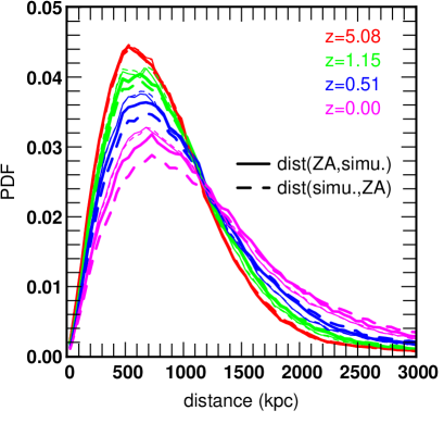
(a) ZA and simulation

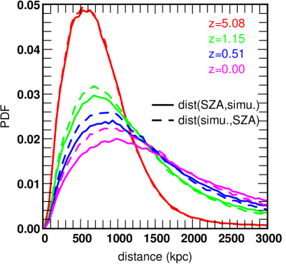
(b) ZA applied to the skeleton (SZA) and simulation

Figure 15: The inter-skeleton distance as defined in the main text and appendix B, applied to the skeletons of the simulation and the Zel’dovich approximation (Figure 15(a)) and the skeletons of the simulation and displaced initial conditions skeleton, SZA (Figure 15(b)). The displacement fields and skeletons are computed after smoothing the field on a scale $L\approx 3.94$ such that $\sigma(L,z=0)=1$, except for SZA, where the displacement field was obtained after smoothing over $L_{l}\approx 8.81$ Mpc, such that $\sigma(L,z=0)=0.5$. The full lines represent the distance from the simulation’s skeleton to the other, while the dotted lines represent the reciprocal distance. The thin lines on Figure 15(a) stand for the case where the effective smoothing introduced by the Zel’dovich approximation is taken into account. Note that SZA PDF is more skewed as the merging/annihilation of filaments is then not taken into account.

3.3 Inter-skeleton pseudo-distance

Let us now define a way to compute a pseudo-distance between two different skeletons (see also Caucci et al. (2008)). In practice, a skeleton ${\cal S}$ is always computed from a sampled density and thus has a maximal resolution $R_{s}$. It can therefore be described, without loss of information, as the union of a set of $N$ straight segments ${\cal S}^{i}$ of size $R_{s}$. We define a pseudo-distance from a skeleton ${\cal S}_{a}$ to a skeleton ${\cal S}_{b}$, ${\cal D}\!\left({\rm a},{\rm b}\right)$, as the probability distribution function (PDF) of the minimal distance from the $N^{a}$ segments ${\cal S}_{a}^{i}$ to any of the $N^{b}$ segments ${\cal S}_{b}^{j}$. In practice, our algorithm applied to a density field sampled on a Cartesian grid naturally leads to a skeleton described as a set of segments of size the order of the sampling resolution. Hence we directly use these segments to compute inter-skeleton distances.

Note that there is no reason, in general, for ${\cal D}\!\left({\rm a},{\rm b}\right)$ to be identical to ${\cal D}\!\left({\rm b},{\rm a}\right)$; this discrepancy, together with the value of the different modes of the PDFs, do in fact quantify the differences between ${\cal S}_{a}$ and ${\cal S}_{b}$ (see appendix B for details on how to interpret pseudo-distances PDFs). The upper and lower panels of Figure 15 present the pseudo distance measurements obtained by comparing ${\cal S}_{\rm simu}$ to ${\cal S}_{\rm ZA}$ and ${\cal S}_{\rm SZA}$ respectively. A close examination of Figure 15(a) confirms the hypothesis we made in previous subsection. First, the high correlation of ${\cal S}_{\rm ZA}$ and ${\cal S}_{\rm simu}$ (bold curves) for any redshift, is demonstrated by the localization of the mode around $d\approx 600h^{-1}$ kpc, well below the smoothing length $L_{\rm NL}=3.94$ Mpc. Second, the asymmetry between the PDFs of ${\cal D}\!\left({\rm ZA},{\rm simu}\right)$ and ${\cal D}\!\left({\rm simu},{\rm ZA}\right)$ follows from the fact that ${\cal S}_{\rm simu}$ has smaller scale filaments that have no counterpart in ${\cal S}_{\rm ZA}$ (the mode intensity is higher for ${\cal D}\!\left({\rm ZA},{\rm simu}\right)$ than ${\cal D}\!\left({\rm simu},{\rm ZA}\right)$). This is exactly what should happen if ${\cal S}_{\rm ZA}$ was effectively smoothed on a scale larger than ${\cal S}_{\rm simu}$. The thin curves, for which the effective Zel’dovich approximation smoothing was taken into account, confirms this, as the asymmetry is completely removed in that case.

It is also interesting to look at the distance PDFs between ${\cal S}_{\rm SZA}$ and ${\cal S}_{\rm simu}$ (see Figure 15(b)). Except for high redshifts ($z=5$), the general intensity of the modes are lower for ${\cal D}\!\left({\rm SZA},{\rm simu}\right)$ than for ${\cal D}\!\left({\rm ZA},{\rm simu}\right)$, suggesting that the Zel’dovich approximation is a better description of the evolution of the filaments on large scales, and that filaments mergers and creation are important processes. The general position of the modes is still comparable, which means that SZA is nonetheless successful in describing the evolution of the general shape of the cosmic web. Also, the asymmetry between ${\cal D}\!\left({\rm SZA},{\rm simu}\right)$ and ${\cal D}\!\left({\rm simu},{\rm SZA}\right)$ suggests that ${\cal S}_{\rm SZA}$ has more small scale filaments than ${\cal S}_{\rm simu}$. These observations confirm our previous assumption that although the cosmic web evolves in a simple inertial way on larger scales (a process captured by SZA), the shrinking and fusion of the more numerous smaller scale filaments is the cause of the general length decrease of the cosmic web (as suggested by a simple visual examination of a $(50h^{-1})^{3}$ ${\rm Mpc}^{3}$ subregion of ${\cal S}_{\rm simu}$, ${\cal S}_{\rm SZA}$ and ${\cal S}_{\rm ZA}$ on Figure 16).

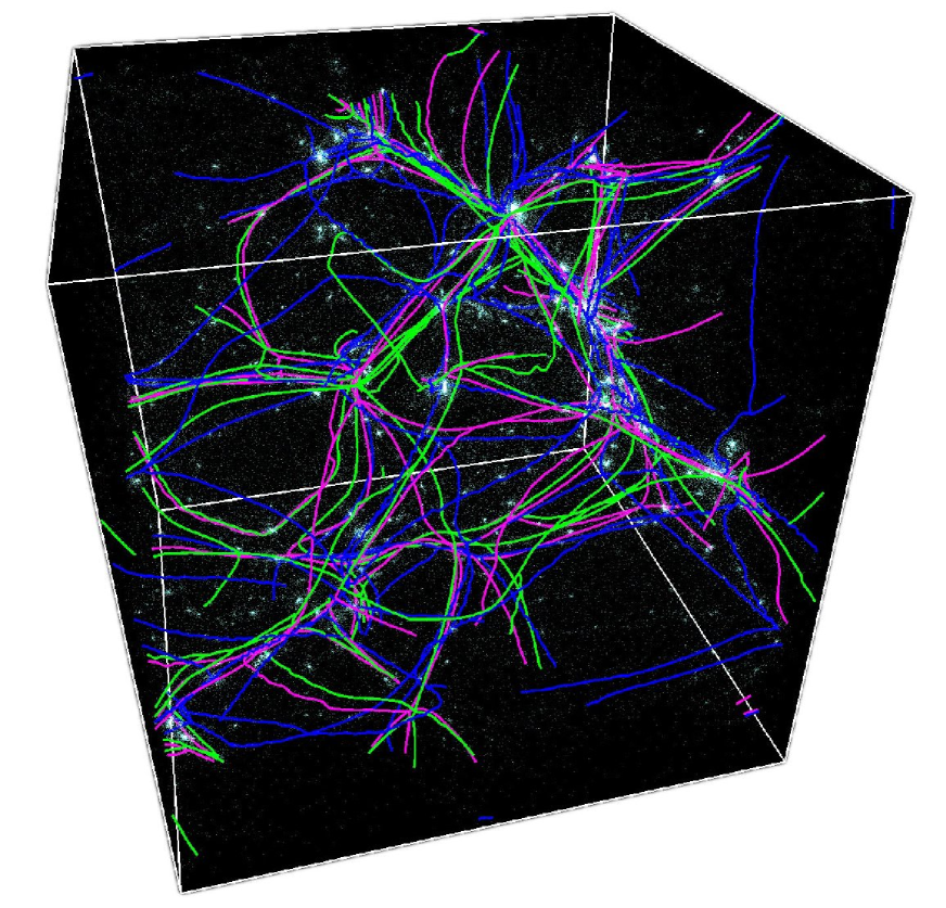
Figure 16: A $(50h^{-1})^{3}$ ${\rm Mpc}^{3}$ section of the $512^{3}$ particles simulation of a $250h^{-1}$ Mpc large box (only $1$ particle every $8$ is displayed). The purple skeleton is ${\cal S}_{\rm simu}(z,L)$ (computed from the simulation), the green one ${\cal S}_{\rm ZA}(z,L_{\rm cor})$ (computed on the Zel’dovich approximation using an effective smoothing length) and the blue one ${\cal S}_{\rm SZA}(z,L_{\rm NL})$ (computed by displacing the skeleton of the initial conditions). The simulation and corrected Zel’dovich approximation skeletons appear to be relatively close to each other and every individual filament has a counterpart in the other skeleton. The blue skeleton, computed from the skeleton Zel’dovich approximation, is more wiggly which reflects the small scale perturbation of the displacement field. Moreover, while many of its filaments have counterpart in the two other skeletons, others do not, as displacing the initial skeleton prevents the merging or disappearance of filaments. This results can be quantitatively measured, as shown on Figure 15 and explained in appendix B.

The above investigation opens the prospect of correcting for the peculiar velocities of galaxies induced by gravitational clustering, and carry an Alcock-Paczynski (AP) test (Alcock & Paczynski, 1979) on the skeleton of the large scale structures of the universe. In short, the AP test compares observed transverse and longitudinal distances to constrain the global geometry of the universe. Galaxy positions are usually observed in redshift space which induces an important distortion between the distances measured along and orthogonally to the line of sight, which plagues the regular AP-test. Our analysis suggests that it is in fact possible to correct through the Zel’dovich approximation for the distortions induced on the cosmic web. Having carried such a correction, we expect that the measure of the anisotropy of the observed skeleton length ratio could yield a good constraint on the value of the cosmological parameters. Note finally that The Zel’dovich mapping smoothed with $L_{\rm cor}$ (see Equation (16)) could be used to generate synthetically sets of extremely large cosmic skeletons probing exotic cosmologies using codes such as mpgrafic (Prunet et al., 2008) to generate the initial conditions and their Zel’dovich displacement. This construction could then be populated with halos and substructure using semi analytical models. Note finally that the total length and the skeleton’s distance are two probes amongst many on how to characterize the difference between two skeletons. Moreover, there are other means to quantify the evolution of the cosmic web. For instance, an interesting statistics would be to find out how often the reconnection of the skeleton occurs as a function of redshift.

4 Discussion and prospects

We have presented a method, based on an improved watershed technique, to efficicently compute the full hierarchy of critical subsets from a density field within spaces of arbitrary dimensions. Our algorithm uses a fast one pass probability propagation scheme that is able to improve significantly the quality of the segmentation by circumventing the discreteness of the sampling. We showed that, following Morse theory, a recursive segmentation of space yields, for a $d$-dimensional space, a succession of $d-1$ $n$-dimensional subspaces that characterize the topology of the density field. In 3D for cosmological matter density distribution, we particularly focused on the 3D subspaces which are the peak and void patches of the field (i.e. the attraction/repulsion pools) and the 1D critical lines which trace the filaments as well as the whole primary cosmic web structure (i.e. a fully-connected, non-local skeleton as defined in Novikov et al. (2006)). For the primary critical lines, we also demonstrated that it is possible to use the probabilities distribution from our algorithm to derive a smooth and differentiable skeleton with a sub-pixel level resolution. Thus this method allows us to consider the cosmic web as a precise physical object and makes it possible to compute any of its properties such as length, curvature, halos connectivity etc…

As an application, we used our algorithm to study the evolution of the cosmic web, while comparing the time evolution of the skeleton (a proxy to the cosmic web) of a simulation, to those corresponding to different versions of its Zel’dovich approximation. We first compared the evolution of the respective lengths of the different skeletons and then introduced a method to compute pseudo-distances between different skeletons. This pseudo distance makes it possible to compare different features of the skeleton such as the size of their filaments and the similarity of their locations. Using these measurements, we showed that two effects were competing, with net result a decrease of the cosmic length with time: a general dilation of the larger scales filaments that could be captured by a simple deformation of the skeleton of the initial conditions on the one hand, and the shrinking, fusion and disappearance of the more numerous smaller scales filaments on the other hand. We also showed that a simple Zel’dovich approximation could accurately capture most features of the evolution of the cosmic web for all scales larger than a few megaparsecs (provided an effective smoothing introduced by the approximation is taken into account). Hence in this context, the skeleton has proven to be a useful tool both for insight and as a quantitative probe and diagnostic. Conversely, the match between the simulated and the mapped skeleton confirms and extends geometrically the (point process elliptical) peak patch theory (Bond & Myers, 1996) since both the peaks and their frontiers (the skeleton in 2D and the peak patch volumes in 3D) are well mapped by the Zel’dovich approximation.

The domain of interest of the skeleton is quite vast and offer the prospect of a number of applications.

From a theoretical point of view, using the points presented in this paper and in Sousbie et al. (2008a), we are presently developing a general theory of the skeleton and its statistical properties (Pogosyan et al., in prep.) that aims to understand the properties of the critical lines of scale invariant Gaussian random fields as mathematical objects. In particular, this companion paper provides quantitative analytic predictions for the length per unit volume (resp. curvature) of the critical lines and its scaling with the shape parameter of the field, and checks successfully the current algorithm against these. In this paper we focussed on the skeleton. One could clearly investigate on the rest of the peak patch hierarchy and measure, say, the surface or volume of the (hyper)-surfaces of the recursion (whose last intersection is given by the primary critical lines). Another interesting issue would be to estimate the fraction of special (degenerate) points which do not satisfy the Morse condition, where the fields behaves pathologically (Pogosyan et al., in prep.).

For instance, one of the shortcoming of the present algorithm concerns special fields where critical lines disappear, a situation which occurs, say, in the context of tracing dendrites in a neural network, or blood vessels within a liver. Note also that there exist other sets of (geometrical) critical lines that are not topological invariants such as the lines of steepest ascent connecting directly minima to maxima which are not accounted for by the present formalism. In contrast, the algorithm is well suited to identify bifurcation points, and the connectivity of the network. In particular, in an astrophysical context, it would be worthwhile to make use of this feature and study statistically how the skeleton connects onto dark matter halos as a function of, say, they mass or spin, and investigate the details of local spin accretion in the context of the cosmic web superhighways, hence completing the spin alignment measurements of Sousbie et al. (2008a) on smaller scales. More generally, the algorithm provides a neat bridge, via the provided connectivity, between the theory of continuous fields on the one hand, and graph theory for discrete networks on the other. This could prove to be of importance in the context of percolation theory. For instance, the percolation threshold can be explained in terms of the properties of the connectivity of the relevant nodes (see e.g. Colombi et al. (2000)).
Here, as argued in section 2.4 we deliberately chose not to consider the issue of shot noise and its consequences on segmentation, for which no definitive solution yet exists, though many improvements have been proposed in the literature (see e.g. Roerdink (1995)). Instead, we followed the approach of Sousbie et al. (2008a), that simply involves convolving the sampled density field with a large enough (in terms of sampling scale) Gaussian kernel so that the field can be considered smooth and differentiable; the probabilistic algorithm allows for the removal of sampling effects and small intensity residual shot noise. In appendix C we show that the corresponding fully connected skeleton is nonetheless quite robust (the core of the network remains quasi unchanged), so long as the SNR is above one. A possible drawback of this method is that it introduces a smoothing scale attached to the skeleton. This is not necessarily a problem in cosmology as the scaling of the skeleton properties with scale yields information on the distribution over these scales. Moreover, one is usually interested by the properties of the skeleton on a given scale (typically larger than the halo scale, a few megaparsecs). Nonetheless, there exist more complex multi-scale sampling and smoothing techniques such as the one presented in Platen et al. (2007) or Colberg (2007) that could straightforwardly be adapted to our implementation. All the algorithm requires is a structured sampling grid where one can recover a one to one pixel neighbourhood (i.e. one needs to be able to find the neighbouring pixels of any pixel and these pixels must have the former as neighbour as well). For instance, we already implemented the algorithm for an Healpix (Górski et al., 2005) pixelisation of the sphere (see Figure 17), while a direct implementation on a delaunay tesselation network is clearly an option.
A natural extension of the theoretical component of this work would be to investigate numerically the properties of the bifurcation points in abstract space or anisotropic settings (see Pogosyan et al. (in prep.) for a theoretical discussion for isotropic Gaussian random fields). For instance, in the context of cosmic structure formation, Hanami (2001), relied on the parallel between the skeleton of the density field in position-time 4D space and in position-scale 4D space to relate the two. In the former, the skeleton is a natural way of computing what is known as a halos merger tree, commonly used in semi-analytical galaxy formation models (see Hatton et al. (2003) for instance): the skeleton traces the evolution of the critical points of the density field in time. The peak theory (Bond & Myers, 1996) tells us that the smoothing scale can be linked to time evolution on scales where gravitational effects remain weakly non-linear. A worthwhile goal is to establish the parallel between the properties of 4D skeleton in this position-smoothing scale space (which can be computed from the Gaussian initial conditions only) and the halo merger tree.Finally, note that classical bifurcation theory is concerned with the evolution of a critical point as a function of a control parameter. In the language of the skeleton, this evolution may correspond to the skeleton in the extended “phase space”.

From the physical and observational point of view, an other interesting venue would be to apply the skeleton to actual galaxy catalogs such as the SDSS (Adelman-McCarthy et al., 2008) to characterize the (universal) statistics of filaments as physical objects, like halos or voids, and describe them in terms of their thickness, length, curvature and environmental properties (galaxies types, halo proximity, color and morphology gradient…), both in virtual and observed catalogs. It could also be used as a diagnosis tool for inverse methods which aim at reconstructing the three dimensional distribution of the IGM from say QSO bundles (Caucci et al., 2008) or upcoming radio surveys (LOFAR, SKA etc…) Clearly the peak patch segmentation developed in this paper will also be useful in the context of the upcoming surveys such as the LSST, or the the SDSS-3 BAO surveys, for instance to identify rare events such as large walls or voids and study their shape. Its application to CMB related full sky data, such as WMAP or Planck should provide insight into, e.g. the level of non Gaussianity in these maps. Similarly, upcoming large scale weak lensing surveys (Dune, SNAP…) could be analysed in terms of these tools (see Pichon et al. (in prep.) for the validation of a reconstruction method in this context). Using the skeleton, the geometry of cold gas accretion that fuel stellar formation in the core of galaxies could be probed. The properties of the distribution of metals on smaller scales could be also investigated using peak patches, to see how they influence galactic properties; one could compare these statistical results to those obtained through WHIM detection by Oxygen emission lines (Aracil et al. (2004) Caucci et al. (2008)). Indeed it has been claimed (see e.g. Ocvirk et al. (2008) Dekel et al. (2008)) that the geometry of the cosmic inflow on a galaxy (its mass, temperature and entropy distribution, the connectivity of the local filaments network etc. ) is strongly correlated to its history and nature.

In closing, let us emphasize again that the scope of application of the algorithm presented in this paper extends well beyond the context of the large scale structure of the universe: it could be used in any scientific of engineering context (medical tomography, geophysics, drilling …) where the geometrical structure of a given field needs to be characterized.

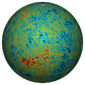
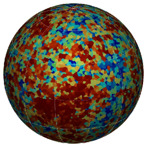
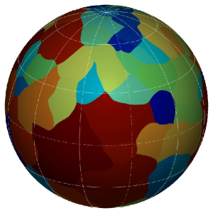
Figure 17: from left to right: the 5 year WMAP release of the CMB temperature map, the corresponding peak patches and the peak patches of the same field smoothed over a FHWM of 420 arcmin. Different colours represent different patches. The algorithm described in section 2 is implemented here on the healpix pixelisation.

Acknowledgements

We thank D. Pogosyan, D. Aubert, J. Devriendt, J. Blaizot, S. Peirani and S. Prunet for fruitful comments during the course of this work, and D. Munro for freely distributing his Yorick programming language and opengl interface (available at http://yorick.sourceforge.net/). This work was carried within the framework of the Horizon project, www.projet-horizon.fr.

Appendix A A generic minimization algorithm

In this appendix, we present a generic algorithm that aims at minimizing a multi-linear scalar function $f(x_{1},..,x_{d})$ of $d$ variables within a polygonal volume, in a $d$-dimensional space, by reducing the problem to finding the respective minima of a set of polynomials of order $d$. It takes as input the location of the minima, $M_{i}^{0}$, of $f(x_{1},..,x_{d})$ on the edges of the square and simply consists in recursively minimizing the value of $f(x_{1},..,x_{d})$ along the lines joining them.

Let us first consider the 2D case illustrated by Figure 18, where the cell is a square. In this case, three minima, $M_{1}^{0}$, $M_{2}^{0}$ and $M_{3}^{0}$ (represented by red crosses) can be easily found on the edges of the square from the linearly interpolated value of $f$ along them. One can then compute the location of the minima along the three lines linking them (the red triangle), noting that because of the multi-linearity of $f$, its value along a line can be expressed as a second order polynomial. One thus obtains $3$ new points, $M_{1}^{1}$, $M_{2}^{1}$ and $M_{3}^{1}$, and the process can be repeated, as represented by the blue and black sets of lines, until convergence to the solution, represented by the blue cross (i.e. when the three points are close enough to each other).

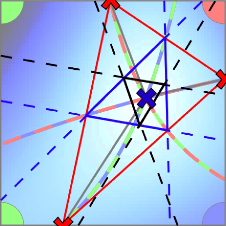
Figure 18: Illustration in the 2D case of the recursive minimization algorithm, applied to the case of Figure 5(b). The reader can refer to the legend of Figure 5 for more details. The scalar field to minimize is represented by the blue shading in the background while its minimum is located at the intersection of the 3 quadrics. The red crosses locate the field minima along the edges while the red, blue and black sets of lines result from the first three recursion steps.

This algorithm can be generalized to the case of the $p$-face of an $n$-cubic cell, $p\leq n$, thus providing the solution over the $p$-face from the $k$ solutions, $M_{i}^{0}\;i\in\{1,..,k\}$ , over the sets of $(p-1)$-faces that are its edges. As explained in section 2.3.3, this algorithm is thus recursively applied to the edges of the cell, starting from the $1$-faces, in the order of their increasing dimensionality. The $j^{th}$ step of the algorithm thus goes as follows:

1. Compute the equations of the $(k)(k-1)/2$ lines joining pairs of $M_{i}^{j-1}$.

2. Evaluate the value of $f(x_{1},..,x_{d})$ at $p+1$ points along these lines using multi-linear interpolation, and fit a polynomial of order $p$.

3. Find the minima of these polynomials that belong to the cell and keep the $k$ lowest among them, with coordinates $M_{i}^{j}$.

4. If these points are all contained in a sphere of radius a given fraction of the cell, stop, else start over.

Note that although only the case of a Cartesian sampling grid was presented here, the algorithm is easily transposable to any type of grid, such as the one produced by Voronoi tessellation on a manifold, which is composed of simplex shape cells.

Appendix B Inter-skeleton pseudo-distance

The inter-skeleton pseudo-distance from one skeleton ${\cal S}_{a}$ to another skeleton ${\cal S}_{b}$ was defined in the main text by the probability distribution function (PDF) of the minimum of the distance from each segment of ${\cal S}_{a}$ to any segments of ${\cal S}_{b}$. In this appendix, we show how this measure can be interpreted using realizations of scale invariant Gaussian random fields (GRFs) with different power spectrum index $n$ (such that $P\left(k\right)\propto k^{-n}$) and different smoothing lengths $L$. All the skeletons that we use were computed from $512^{3}$ pixels realizations of GRFs, smoothed over a scale $L=8$ pixels or $L_{L}=16$ pixels. These scales are defined as the width of the Gaussian kernel that we used to smooth the fields and the value of $L$ roughly corresponds, in number of pixels, to the smoothing scale we used in the main text, $L_{\rm NL}$. A total of six different skeletons were computed:

• ${\cal S}_{\rm GRF0}$ and ${\cal S}_{\rm GRF0^{\prime}}$: skeletons computed from two realizations (GRF0 and ${\rm GRF0}^{\prime}$) of GRFs with spectral index $n=0$, smoothed over a scale $L=8$ pixels.
  

• ${\cal S}_{\rm GRF3}$ and ${\cal S}_{\rm GRF3^{\prime}}$: skeletons computed from two realizations (GRF3 and ${\rm GRF3}^{\prime}$) of GRFs with spectral index $n=3$, smoothed over a scale $L=8$ pixels.
  

• ${\cal S}_{\rm GRF0_{T}}$: this skeleton was computed from the field GRF0, smoothed on scale $L$. The resulting skeleton was then translated by ${\bf v}=\left(L/2,0,0\right)$.
  

• ${\cal S}_{\rm GRF0_{L}}$: this skeleton was computed from the field GRF0, smoothed on scale $L_{L}=2L=16$ pixels.
  

(a) $n=0$

(b) $n=3$

(c) $n=0$ and $n=3$

(d) $n=0$ and its translation

(e) $n=0$, different smoothing lengths

(f) $n=0$, translation and different smoothing lengths

Figure 19: Measures of the inter-skeleton pseudo distances for Gaussian random fields with different power spectrum index $n$ and smoothing length $L$. These plots show how the pseudo-distances measurements can be used to assess the discrepancies between two skeletons.

Figure 19 presents the different pseudo-distances between these skeletons, ${\cal D}\!\left({\rm a},{\rm b}\right)$. Figures 19(a) and 19(b) present the results obtained when comparing uncorrelated fields (i.e. different realizations of GRFs). As expected in that case, ${\cal D}\!\left({\rm GRF0},{\rm GRF0^{\prime}}\right)={\cal D}\!\left({\rm GRF0^{\prime}},{\rm GRF0}\right)$ and ${\cal D}\!\left({\rm GRF3},{\rm GRF3^{\prime}}\right)={\cal D}\!\left({\rm GRF3^{\prime}},{\rm GRF3}\right)$ and the position of the mode is about the smoothing length. One should also note that the mode intensity differs between $n=0$ and $n=3$, which can be explained by the fact that in the latter case, small scale fluctuations are suppressed together with smaller scale filaments, thus making it less probable for a segment of one realization to be very close to one of the other realization. Figure 19(c) shows that these pseudo distance measurements make it possible to distinguish the different nature of two skeletons. In fact, whereas ${\cal S}_{\rm GRF0}$ has filaments on any scales, only the larger scales are present in ${\cal S}_{\rm GRF3}$, which translates into an asymmetry between ${\cal D}\!\left({\rm GRF0},{\rm GRF3}\right)$ and ${\cal D}\!\left({\rm GRF3},{\rm GRF0}\right)$. Whereas in the first case, there is no reason why every segment of ${\cal S}_{\rm GRF0}$ should be close to a segment of ${\cal S}_{\rm GRF3}$, the reciprocal is not true : ${\cal S}_{\rm GRF0}$ spreads on all scales and every segment of ${\cal S}_{\rm GRF3}$ should be as close as any other from a segment of ${\cal S}_{\rm GRF0}$ (hence the higher intensity of the mode for ${\cal D}\!\left({\rm GRF3},{\rm GRF0}\right)$). When comparing a skeleton ${\cal S}_{\rm a}$ with less filaments to a skeleton ${\cal S}_{\rm b}$ with more filaments, the intensity of the mode is thus expected to be higher for ${\cal D}\!\left({\rm a},{\rm b}\right)$ than for ${\cal D}\!\left({\rm b},{\rm a}\right)$.

This observation is confirmed by Figure 19(e) where ${\cal S}_{\rm GRF0_{L}}$ is compared to ${\cal S}_{\rm GRF0}$, which has small scale filaments that ${\cal S}_{\rm GRF0_{L}}$ does not have. But in that case, the two skeletons are correlated as only the smoothing length changes. This results in a higher intensity of the mode of ${\cal D}\!\left({\rm GRF0_{L}},{\rm GRF0}\right)$: the larger scale filaments are present in both skeletons. It also results in a shift in the position of the mode, located at a distance smaller than the smoothing length. Figure 19(d) illustrates the case of a simple translation of length half the smoothing length $L$: in that case, both PDFs are identical and a very asymmetric and high intensity mode is present at distance $L/2$. Finally, it is also interesting to note that the comparison of ${\cal S}_{\rm GRF0_{L}}$ to ${\cal S}_{\rm GRF0_{T}}$ almost gives the exact same result as the one for ${\cal S}_{\rm GRF0_{L}}$ to ${\cal S}_{\rm GRF0}$ and it is difficult to distinguish one from the other.

Appendix C Robustness of Fully connected skeleton

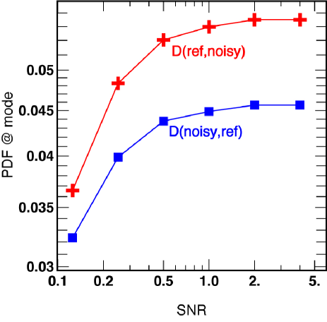
Figure 20: The evolution of the PDF of distances at the mode as a function of the SNR of a noisy field. Here the distance is computed between the reference skeleton and its noisy counter part. For SNR above one, only small differences between weak filaments account for the difference between the two distances. Conversely, for more noisy fields, the fraction of match between the two skeleton drops.

In order to investigate the robustness of the fully connected skeleton with respect to small changes in the underlying field, the following experiment is carried. A given 2D white random field of size $4096^{2}$ is generated. It is then smoothed over 10 pixels, and its reference skeleton, ${\cal S}_{\rm ref}$ is computed. A white random field of amplitude SNR is added to the reference field, and the corresponding skeleton, ${\cal S}_{\rm SNR}$, is computed after smoothing over 10 pixels. The PDF of the pseudo-distances ${\cal D}\!\left({\rm{\cal S}_{\rm ref}},{\rm{\cal S}_{SNR}}\right)$ and ${\cal D}\!\left({\rm{\cal S}_{\rm SNR}},{\rm{\cal S}_{ref}}\right)$ is then calculated (see Appendix B). The distance at the maximum (its mode) of both PDF remains unchanged for all the SNR considered ($1/8,1/4,1/2,1,2,4$), which demonstrates that the core of the skeleton is quite robust: the reference skeleton is always shadowed by its noisy counter part. The amplitude of the PDF at its maximum is plotted in Figure 20. This amplitude is sensitive to the high distance tail of mismatch between the two skeleton since the PDF is normalized. In short, within the network there is a small subset of filaments which are sensitive to any small variation of the field. For the vast majority of the network, the skeleton is globally only weakly affected by changes of the underlying field so long as the amplitude of the change has a SNR above one. When the SNR drops bellow one, spurious filaments occur more and more. The discrepancy between the two plateaux at larger SNR reflects the fact that weaker filaments will occur somewhat randomly from one realisation to another, depending on very small details in the field.

References

- Adelman-McCarthy et al. (2008) Adelman-McCarthy, J. K., et al. 2008, ApJ Sup., 175, 297
- Alcock & Paczynski (1979) Alcock, C., & Paczynski, B. 1979, Nature, 281, 358
- Aracil et al. (2004) Aracil B., Petitjean P., Pichon C., Bergeron J., 2004, A&A, 419, 811
- Aragón-Calvo et al. (2007) Aragón-Calvo, M. A., Jones, B. J. T., van de Weygaert, R., & van der Hulst, J. M. 2007, A&A, 474, 315
- Aragón-Calvo et al. (2007) Aragón-Calvo, M. A., van de Weygaert, R., Jones, B. J. T., & van der Hulst, J. M. 2007, ApJ Let., 655, L5
- Aubert & Pichon (2006) Aubert, D., & Pichon, C. 2006, EAS Publications Series, 20, 37
- Aubert et al. (2004) Aubert, D., Pichon, C., & Colombi, S. 2004, MNRAS, 352, 376
- Barrow et al. (1985) Barrow, J. D., Bhavsar, S. P., & Sonoda, D. H. 1985, MNRAS, 216, 17
- Bertschinger (1985) Bertschinger, E. 1985, ApJ Sup., 58, 1
- Beucher & Lantuejoul (1979) Beucher S., Lantuejoul C., 1979, in Proceedings International Workshop on Image Processing, CCETT/IRISA, Rennes, France
- Beucher & Meyer (1993) Beucher S., Meyer F., 1993, Mathematical Morphology in Image Processing , ed. M. Dekker, New York, Ch. 12, 433
- Bharadwaj et al. (2000) Bharadwaj, S., Sahni, V., Sathyaprakash, B. S., Shandarin, S. F., & Yess, C. 2000, ApJ, 528, 21
- Bond & Myers (1996) Bond, J. R., & Myers, S. T. 1996, ApJ Sup., 103, 1
- Bond et al. (1991) Bond, J. R., Cole, S., Efstathiou, G., & Kaiser, N. 1991, ApJ, 379, 440
- Colberg (2007) Colberg, J. M. 2007, MNRAS, 375, 337
- Coles et al. (1993) Coles, P., Melott, A. L., & Shandarin, S. F. 1993, MNRAS, 260, 765
- Colless et al. (2003) Colless, M., et al. 2003, ArXiv Astrophysics e-prints, arXiv:astro-ph/0306581
- Colombi et al. (2000) Colombi, S., Pogosyan, D., & Souradeep, T. 2000, Physical Review Letters, 85, 5515
- Caucci et al. (2008) Caucci S., Colombi S., Pichon C., Rollinde E., Petitjean P., Sousbie T., 2008, MNRAS in press, pp 000–000
- Dekel et al. (2008) Dekel A., Birnboim Y., Engel G., Freundlich J., Goerdt T., Mumcuoglu M., Neistein E., Pichon C., Teyssier R., Zinger E., 2008, ArXiv e-prints, 808
- de Lapparent et al. (1986) de Lapparent, V., Geller, M. J., & Huchra, J. P. 1986, ApJ Let., 302, L1
- El-Ad & Piran (1997) El-Ad, H., & Piran, T. 1997, ApJ, 491, 421
- Forero-Romero et al. (2008) Forero-Romero, J. E., Hoffman, Y., Gottloeber, S., Klypin, A., & Yepes, G. 2008, arXiv:0809.4135
- Gottloeber (1998) Gottloeber, S. 1998, Large Scale Structure: Tracks and Traces, 43
- Górski et al. (2005) Górski K. M., Hivon E., Banday A. J., Wandelt B. D., Hansen F. K., Reinecke M., Bartelmann M., 2005, ApJ, 622, 759
- Graham et al. (1995) Graham, M. J., Clowes, R. G., & Campusano, L. E. 1995, MNRAS, 275, 790
- Hahn et al. (2007) Hahn, O., Carollo, C. M., Porciani, C., & Dekel, A. 2007, MNRAS, 381, 41
- Hanami (2001) Hanami, H. 2001, MNRAS, 327, 721
- Harker et al. (2006) Harker, G., Cole, S., Helly, J., Frenk, C., & Jenkins, A. 2006, MNRAS, 367, 1039
- Hatton et al. (2003) Hatton S., Devriendt J. E. G., Ninin S., Bouchet F. R., Guiderdoni B., Vibert D., 2003, MNRAS, 343, 75
- Hoffman & Shaham (1982) Hoffman, Y., & Shaham, J. 1982, ApJ Let., 262, L23
- Huchra & Geller (1982) Huchra, J. P., & Geller, M. J. 1982, ApJ, 257, 423
- Icke (1984) Icke, V. 1984, MNRAS, 206, 1P
- Jost (1995) Jost , Jorgen., Riemannian Geometry and Geometric Analysis, Fourth Edition, 1995, Springer
- Kirshner et al. (1981) Kirshner, R. P., Oemler, A., Jr., Schechter, P. L., & Shectman, S. A. 1981, ApJ Let., 248, L57
- Kofman et al. (1992) Kofman, L., Pogosyan, D., Shandarin, S. F., & Melott0, A. L. 1992, ApJ, 393, 437
- Lacey & Cole (1993) Lacey, C., & Cole, S. 1993, MNRAS, 262, 627
- Martinez & Saar (2002) Martinez, V., & Saar, E. 2002, Proc. SPIE, 4847, 86
- Merritt et al. (2006) Merritt, D., Graham, A. W., Moore, B., Diemand, J., & Terzić, B. 2006, AJ, 132, 2685
- Milnor (1963) Milnor, J., 1963, Morse Theory (Princeton University, Princeton, NJ)
- Navarro et al. (1997) Navarro, J. F., Frenk, C. S., & White, S. D. M. 1997, ApJ, 490, 493
- Neyrinck (2008) Neyrinck, M. C. 2008, MNRAS, 386, 2101
- Neyrinck et al. (2005) Neyrinck, M. C., Gnedin, N. Y., & Hamilton, A. J. S. 2005, MNRAS, 356, 1222
- Novikov et al. (2006) Novikov, D., Colombi, S., & Doré, O. 2006, MNRAS, 366, 1201
- Ocvirk et al. (2008) Ocvirk P., Pichon C., Teyssier R., 2008, ArXiv e-prints, 803
- Peebles (1980) Peebles, P. J. E. 1980, Research supported by the National Science Foundation. Princeton, N.J., Princeton University Press, 1980. 435 p.,
- Peebles (1993) Peebles, P. J. E. 1993, Princeton Series in Physics, Princeton, NJ: Princeton University Press, —c1993,
- Pichon et al. (2001) Pichon C., Vergely J. L., Rollinde E., Colombi S., Petitjean P., 2001, MNRAS, 326, 597
- Pichon et al. (in prep.) Pichon C., Thiébaut E., Prunet S., Benabed K., Sousbie,T., Teyssier R., Colombi S. in prep.
- Pogosyan et al. (in prep.) Pogosyan D., Pichon C., Prunet S., Gay C., Sousbie,T., Colombi S. in prep.
- Platen et al. (2007) Platen, E., van de Weygaert, R., & Jones, B. J. T. 2007, MNRAS, 380, 551
- Prunet et al. (2008) Prunet S., Pichon C., Aubert D., Pogosyan D., Teyssier R., Gottloeber S., 2008, ArXiv e-prints, 804
- Roerdink (1995) Jos, B. T. M., Roerdink & Arnold Meijster, 2001, Fundamenta informaticae, 41, 187-228
- Sahni et al. (1998) Sahni, V., Sathyaprakash, B. S., & Shandarin, S. F. 1998, ApJ Let., 495, L5
- Sathyaprakash et al. (1996) Sathyaprakash, B. S., Sahni, V., & Shandarin, S. F. 1996, ApJ Let., 462, L5
- Sheth (1998) Sheth, R. K. 1998, MNRAS, 300, 1057
- Sousbie et al. (2008a) Sousbie, T., Pichon, C., Colombi, S., Novikov, D., & Pogosyan, D. 2008a, MNRAS, 383, 1655
- Sousbie et al. (2008b) Sousbie, T., Pichon, C., Courtois, H., Colombi, S., & Novikov, D. 2008b, ApJ Let., 672, L1
- Springel (2005) Springel, V. 2005, MNRAS, 364, 1105
- Springel et al. (2001) Springel, V., White, S. D. M., Tormen, G., & Kauffmann, G. 2001, MNRAS, 328, 726
- Stoica et al. (2005) Stoica, R. S., Martínez, V. J., Mateu, J., & Saar, E. 2005, A&A, 434, 423
- Teyssier et al. (2008) Teyssier, R, Pires, S, Prunet, S, Aubert, D. Pichon, C Prunet, Amara, A Benabed, K Colombi, S Refregier, A. & Starck, J.L. 2008, submitted.
- van de Weygaert & Schaap (2007) van de Weygaert, R., & Schaap, W. 2007, ArXiv e-prints, 708, arXiv:0708.1441
- Wang et al. (2007) Wang, H. Y., Mo, H. J., & Jing, Y. P. 2007, MNRAS, 375, 633
- Zel’Dovich (1970) Zel’Dovich, Y. B. 1970, A&A, 5, 84