Enlightening the structure and dynamics of Abell 1942.

Abstract

Aims. We present a dynamical analysis of the galaxy cluster Abell 1942 based on a set of 128 velocities obtained at the European Southern Observatory.

Methods. Data on individual galaxies are presented and the accuracy of the determined velocities is discussed as well as some properties of the cluster. We have also made use of publicly available Chandra X-ray data.

Results. We obtained an improved mean redshift value $z=0.22513\pm 0.0008$ and velocity dispersion $\sigma=908^{+147}_{-139}\ {\rm km\,s^{-1}}$. Our analysis indicates that inside a radius of $\sim 1.5h_{70}^{-1}\,$Mpc ($\sim 7\,$arcmin) the cluster is well relaxed, without any remarkable feature and the X-ray emission traces fairly well the galaxy distribution. Two possible optical substructures are seen at $\sim 5\,$arcmin from the centre towards the Northwest and the Southwest direction, but are not confirmed by the velocity field. These clumps are however, kinematically bound to the main structure of Abell 1942. X-ray spectroscopic analysis of Chandra data resulted in a temperature $kT=5.5\pm 0.5\,$keV and metal abundance $Z=0.33\pm 0.15Z_{\odot}$. The velocity dispersion corresponding to this temperature using the $T_{X}$–$\sigma$ scaling relation is in good agreement with the measured galaxies velocities. Our photometric redshift analysis suggests that the weak lensing signal observed at the south of the cluster and previously attributed to a “dark clump”, is produced by background sources, possibly distributed as a filamentary structure.

1 Introduction

In the hierarchical $\Lambda$CDM scenario for structure formation, clusters of galaxies are the largest coherent and gravitationally bound structures in the Universe, growing by accretion of nearby galaxy groups or even other clusters. These newcomers are often observed as substructures in the galaxy distribution and, indeed, substructures have been detected in a significant fraction of galaxy clusters (e.g., Flin & Krywult 2006). Clusters can then be used to trace the cosmological evolution of structure with time and to constrain cosmological parameters (e.g., Richstone et al. 1992; Kauffmann & White 1993).

However, clusters comprise a diverse family, presenting a large range of structural behaviour and, in order to be useful as cosmological probes, the structural and dynamical properties of individual systems should be determined. Clusters are also complex entities, containing both baryonic and non-baryonic matter. In the case of the former, most of the baryons occupy the cluster volume in the form of a hot gas emitting in X-rays. Consequently, studies of galaxy clusters aiming to unveil their actual properties are greatly benefited by multiwavelength observations, in particular in X-rays for the gas and in the optical for the galaxies and even the dark matter.

Here we present a study of the cluster of galaxies Abell 1942. It has richness class 3 and Bautz-Morgan type III. It is of particular interest since it has at first glance a quite symmetrical morphology, similar to Abell 586 which can be used as a laboratory to test different mass estimators and to analyze its dynamics (as in Cypriano et al. 2005). This cluster was observed in X-ray by several satellites, ASCA, ROSAT, and Chandra (see Section 4, below). Finally, A1942 has receive some attention because a putative mass concentration would have been detected by its shear effect at 7 arcmin southward from the cluster centre, with no obvious concentration of bright galaxies at this location (Erben et al. 2000; von der Linden et al. 2006): the dark clump. A ROSAT-HRI image was also analyzed by the same authors, showing that the brightest peak of the X-ray emission corresponds with the cluster centre and its central galaxy. A weak secondary source was also detected at 1 arcmin from the mass concentration. Using ASCA data, White (2000) gives 2 temperatures for this cluster: 5.6 keV for a broad band single temperature fit, and 15.6 keV for a cooling-flow fit, which would corresponds to a velocity dispersion $\simeq 1800\leavevmode\nobreak\ \ {\rm km\,s^{-1}}$ and also a huge cooling flow of 817 $M_{\odot}$/year.

From the optical data, only 2 velocities of galaxy members were available, one being the radio-source PKS 1435+038 (Kristian et al. 1978). Moreover, a deep image of the cluster centre (Smail et al. 1991) shows the existence of a few lensed arcs, with one being close to the central galaxy. Up to now, no detailed lens model is available to study the central mass distribution.

In this paper, we analyze Abell 1942 from its photometric, spectroscopic and X-ray properties. In Section 2, we give evidence of the structure and substructures of the cluster from its photometric data. Section 3 presents the spectroscopic survey of the cluster galaxies in order to study the velocity dispersion in the cluster centre, as well as its variations with the radius until the measured limit of the shear up to 8 arcmin (equivalent to a radius of $1.7h^{-1}_{70}$ Mpc at the cluster redshift). In Section 4 we analyze the X-ray data. The velocity analysis is detailed in Section 5. With such a set of velocities we build in Section 6 a detailed image of the cluster dynamics and mass distribution. Moreover we analyze the velocity distribution of the galaxies located close to the mass concentration area in order to know its nature as distant cluster or concentration of matter associated with the main cluster. We adopt here, whenever necessary, $H_{0}=70\,h_{70}\ {\rm km\,s^{-1}}$Mpc^-1, $\Omega_{M}=0.3$ and $\Omega_{\Lambda}=0.7$.

2 Abell 1942 photometric data

The Abell 1942 cluster of galaxies is within the area observed by the Sloan Digital Sky Survey (SDSS) . In this paper we adopt the photometric data from its Data Release Six. Fig. 1 shows a $18\times 18$ arcmin square SDSS image centered at the cluster centre [assumed to be at the position of the brightest cluster galaxy, $m_{r}=16.23$, at at R.A. $14^{\rm h}\,38^{\rm m}\,21.9^{\rm s}$, Dec $+03^{o}\leavevmode\nobreak\ 40^{\prime}\leavevmode\nobreak\ 13^{\prime\prime}$(J2000)] and extending to the South to show the region where a dark mass concentration would have been detected (Erben et al. 2000).

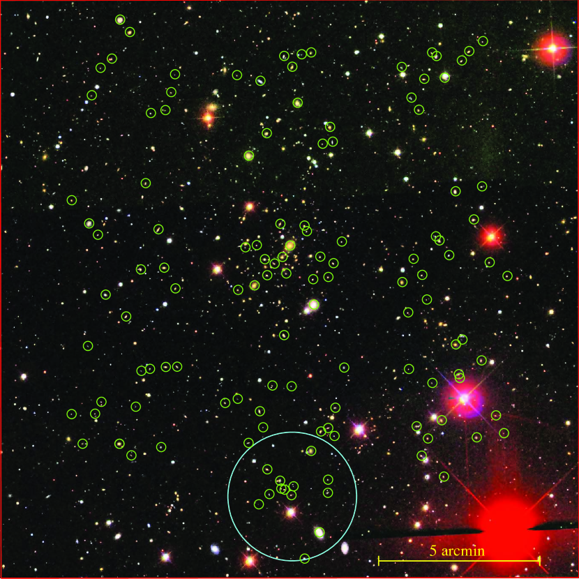
Figure 1: A $18\times 18$ arcmin true colour image from the SDSS centered at the cluster centre. The larger circle, with 2 arcmin radius, corresponds to the dark matter clump region suggested by Erben et al. (2000). Small circles superimposed to galaxy images correspond to the spectroscopic observations reported in this work

Smail et al. (1991) announced the presence of a lensed arc candidate in the cluster centre from $V$ CCD frames taken on the Danish 1.5m telescope at La Silla. During our observations, we also obtained $V$ images which show the centre resolved in independent components with the lensed arc clearly visible. This image is shown in Fig. 2, to which we superimposed the 21cm emission isophotes from the VLA-FIRST (Faint Images of the Radio Sky at Twenty-centimeters) survey (Becker et al. 1994).

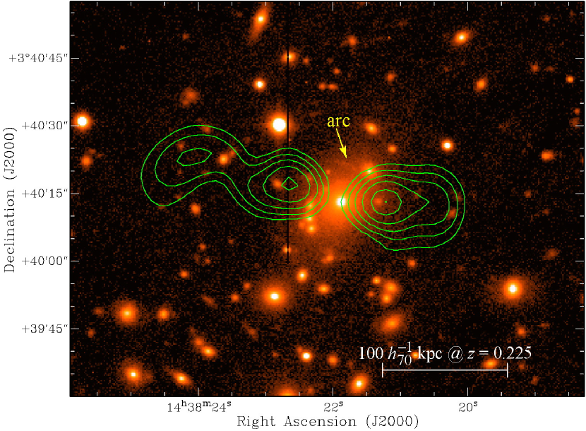
Figure 2: A $V$-band image of the central part of the A1942 cluster taken with EFOSC at the 3.60m ESO telescope. The gravitational arc is indicated by the arrow. The green contours are isophotes of the 21cm VLA-FIRST, logarithmically spaced. The absence of a head-tail radio morphology indicates that the brightest cluster galaxy is at rest with respect to the intracluster gas.

Within the region shown in Fig. 1, there are 674 galaxies with dereddened $r$ magnitudes between 15.36 and 21.0, 17 of them with spectroscopic redshifts in the SDSS database. To this sample we added 128 new spectroscopic redshifts, 9 of them in common with SDSS. About 11 of these new redshifts are in a 200 arcsec side square region centered on the putative dark clump claimed by Erben et al. (2000).

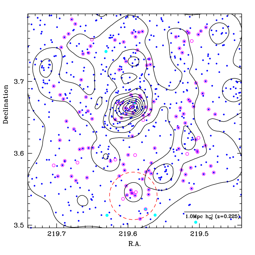
Figure 3: The projected density map of the galaxies brighter than $m_{r}=21.0$ in the 18 arcmin field of Fig. 1. Filled circles denote SDSS galaxies with $m_{r}\leq 21.0$, with larger (cyan) circles for the brightest ones: $14.19\leq m_{r}\leq m_{r_{1}}$, with $m_{r_{1}}=16.23$. Open circles denotes galaxies with measured spectroscopic redshifts. Notice that some of these galaxies are fainter than the $21^{\rm mag}$ limit (see Table 1). The dashed circle encloses the region of the alleged dark clump of Erben et al. (2000). Contours are equally spaced by $\Delta_{\Sigma}=0.4$ with highest levels at $\Sigma_{max}=3.81$, with $\Sigma$ in units of $10^{-3}\rm{gal\leavevmode\nobreak\ arcsec^{-2}}$.

Fig. 3 shows the contour map of the projected density of the 674 galaxies brighter than $m_{r}=21.0$. We adopt this magnitude limit because of our photometric redshifts are reliable up to this value (see Section 5.2). The centre of the cluster appears clearly at $R.A.=219.596^{\circ},Dec=+3.663^{\circ},\leavevmode\nobreak\ \sim 30arcsec$ SE from the dominant cluster galaxy $(219.591^{\circ},+3.670^{\circ})$. The isodensity contours seems slightly elongated in the NW-SE direction, with no significant substructures except perhaps to the north of the cluster centre. At SW ($\simeq 219.54^{\circ}$, $+3.63^{\circ}$) we find a not very significant overdensity which could be identified to the “C” component noticed by Erben et al. (2000) in their figure 10. A small concentration of galaxies is also seen in the region of the alleged dark clump (dashed circle in Fig. 3). We will return to this point in Section 5.2.

3 Spectroscopic observations and Data Reductions

The A1942 spectra used in this paper have been obtained with the 3.60m telescope at ESO-La Silla (Chile) in two runs during a total of ten half-nights from 5 to 10 June 2005 and 30 April to 3 May 2006 (with 4 cloudy nights). A $14.5\times 14.5$ arcmin field centered at the brightest cluster galaxy was tiled into 9 ($3\times 3$) adjacent $5.4\times 5.4$ arcmin fields with a 34 arcsec overlap between them. A 10th field towards the South was added, corresponding to the location of the dark clump (these fields are shown in Fig. 11 below). The instrumentation used was the ESO Faint Object Spectrograph and Camera (EFOSC) with the grism 8 giving a dispersion of 0.99Å/pix.

The targets were preferentially selected from a SDSS sample of 327 galaxies brighter than (undereddened) $m_{r}=20.5$, from which only 97 were picked out given the constraints of the FOV’s of EFOSC. In order to fill the spectroscopic masks with punched slitlets, we added to our list 98 galaxies candidates (as classified by SDSS), fainter than this limit, totalizing 195 targets. Standard stars were also observed during each night for flux calibration of the spectra.

The data reduction was carried out with IRAF using the MULTIRED package. Radial velocities have been determined using the cross-correlation technique (Tonry & Davis 1979) implemented in the RVSAO package (Kurtz et al. 1991; Mink et al. 1995) with radial velocity standards obtained from observations of late-type stars and previously well-studied galaxies.

About 141 of the 195 observed spectra had S/N high enough to allow redshift estimates. About 14 of them were found to be stars. We were thus left with a total of 128 galaxies with measured redshifts, one of which being detected as a possible binary system (galaxies #113 and #116 in Table A.1). About 9 of these spectra are in common with SDSS. About 117 of these are situated in the central square region of 14.5 arcmin side, whereas the remaining 11 are located in a 5.4 arcmin side square field centered on the on the putative dark clump claimed by Erben et al. (2000).

Table A.1 lists positions, dereddened magnitudes $u$, $g$, $r$, $i$ and $z$ (SDSS database), photometric redshifts and errors (see Section 5.2 and the Appendix) and the heliocentric spectroscopic redshifts from the present work. Redshifts errors were derived following Tonry & Davis (1979). The values of their R statistics (defined as the ratio of the correlation peak height to the amplitude of the antisymmetric noise) are listed in the $notes$ column.

3.1 The Completeness of the Spectroscopic Sample

We estimated the completeness of the spectroscopic sample as a function of the magnitude as the ratio of cumulative counts of the spectroscopic samples to that of the photometric ones, $N_{spec}(<m_{r})/N_{phot}(<m_{r})$, all computed within the square 14.5 arcmin side region containing most of our spectral data. The results are displayed in Fig. 4, together with the magnitude distribution of the photometric sample. The completeness was computed both for the entire 14.5 $\times$ 14.5 arcmin region over which the photometric sample was defined (light continuous lines), and over a central circular region of 350 arcsec radius (red continuous lines) which roughly corresponds to the region where the X-ray emission is detected (Section 4). Following the results of Paolillo et al. (2001), the mean $M^{*}$-magnitude of rich Abell clusters is $M^{*}_{r}=-21.24$ (after applying a $0.2^{\rm mag}$ correction between his DPOSS magnitudes and the SDSS magnitudes used here) which, at the redshift of A1942 (see Section 5), $z=0.225$, gives $m^{*}_{r}=19.00$, indicated by an arrow line in Fig. 4.

From this plot it can be seen that the spectroscopic data, which samples nearly uniformly the entire 14.5 $\times$ 14.5 arcmin region, is highly incomplete for magnitudes fainter than $m_{r}\sim 18$. Of course this is due to the clustering of galaxies on the very centre of the region, as it may readily seen in Fig. 4 by comparing the completeness of the central circular region defining the virialized cluster ($\sim 40\%$ at $m_{r}\sim m^{*}_{r}$), to that of its complementary region ($\sim 63\%$ at $m_{r}\sim m^{*}_{r}$; blue continuous lines).

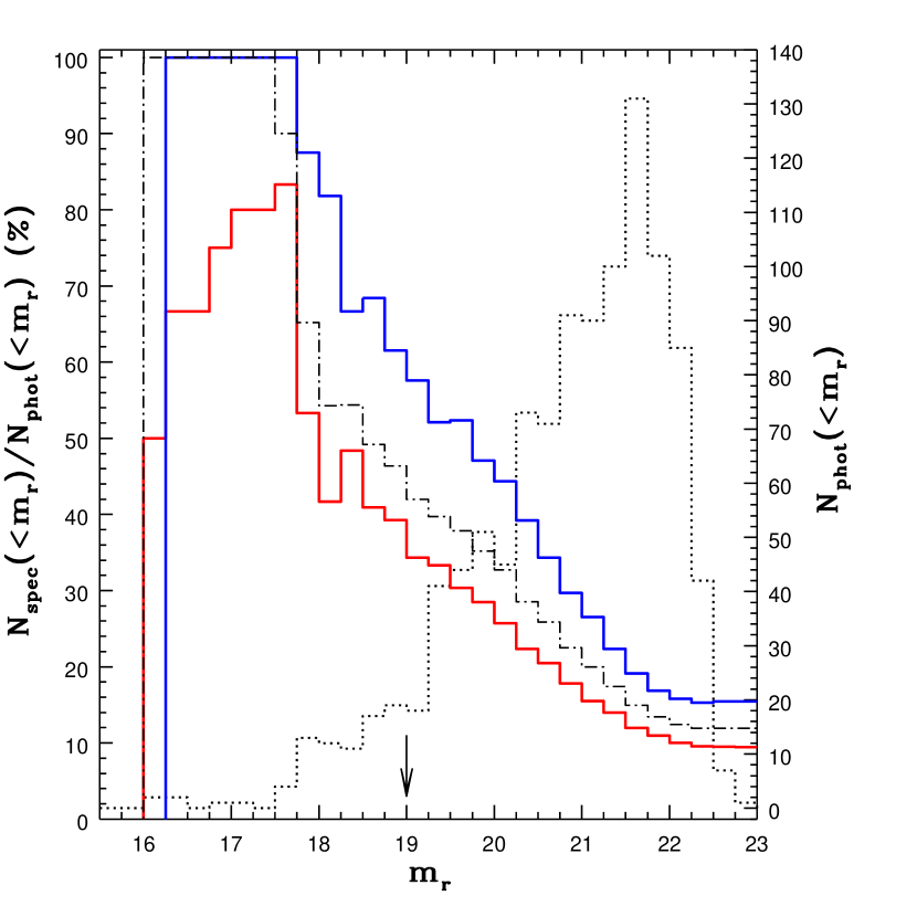
Figure 4: The completeness of the spectroscopic sample as a function of magnitude. Dot-dashed lines: square region 14.5 arcmin side centered in the cluster. Red continuous lines: central circular region of radius 350 arcsec. Blue continuous line: its complementary region. Dotted lines: the luminosity distribution of galaxies of the photometric sample, with values been read in the right vertical axis. The arrow points at the predicted value of $M^{*}$ for an Abell cluster at this redshift.

4 X-ray data

Abell 1942 was first observed by the Einstein satellite Image Proportional Counter (IPC) in 1979 and 1980. Then, it was again observed both by the ROSAT High Resolution Imager (HRI) and ASCA in 1995. In 2003, a 58.3 ks exposure was acquired with Chandra Advanced CCD Imaging Spectrometer-Imager (ACIS-I) detector (ObsID 3290, PI. G. P. Garmire). In 2007 Abell 1942 was again observed by Chandra but only for 5.18 ks. We have downloaded only the ObsID 3290 observation from Chandra X-ray Centre (CXC) archives in order to analyze it.

The morphology of the X-ray emission observed by Chandra was already analyzed by von der Linden et al. (2006), paying close attention to the region of the putative dark clump. Contrary to Erben et al. (2000) analysis based on ROSAT data, they do not detect any significant extended X-ray emission at the supposed location of the dark clump with Chandra data.

Here, we concentrate on the X-ray analysis of the cluster itself which was so far neglected. The data, taken in Very Faint mode, were reduced using CIAO version 3.4 following the Standard Data Processing, producing new level 1 and 2 event files. The level 2 event file was further filtered, keeping only events with grades 0, 2, 3, 4 and 6. We checked that no afterglow was present and applied the Good Time Intervals (GTI) supplied by the pipeline. Only some mild background flares were observed and the corresponding time intervals were filtered away. The final total livetime is 54.66 ks.

We have used the CTI-corrected ACIS background event files (“blank-sky”), produced by the ACIS calibration team, available from the calibration data base (CALDB). The background events were filtered, keeping the same grades as the source events, and then were reprojected to match the sky coordinates of Abell 1942 ACIS-I observation.

We restricted our analysis to the range [0.3–7.0 keV], since above $\sim 7.0$ keV, the X-ray observation is largely dominated by the particle background.

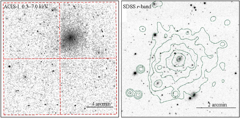
Figure 5: Left: Chandra ACIS-I image of the cluster. Also shown for reference is the position of ACIS-I four CCDs (red dashed lines). Right: SDSS $r$-band image of the central region with X-ray isophotes contours superposed (green solid lines).

4.1 Spectral analysis

For the spectral analysis, we have computed the weighted redistribution and ancillary files (RMF and ARF) using the tasks mkrmf and mkwarf from CIAO. These tasks take into account the extended nature of the X-ray emission. Background spectra were constructed from the blank-sky event files and were extracted at the same regions (in detector coordinates) as the source spectra that we want to fit.

The spectral fits were done using xspec v11.3.2. The X-ray spectrum of each extraction region was modelled as being produced by a single temperature plasma and we employed the mekal model (Kaastra & Mewe 1993; Liedahl et al. 1995). The photoelectric absorption – mainly due to neutral hydrogen – was computed using the cross-sections given by Balucinska-Church & McCammon (1992), available in xspec. We have used metal abundances (metallicities) scaled to Anders & Grevesse (1989) solar values.

The overall spectrum was extracted within a circular region of 78 arcsec ($280h_{70}^{-1}$ kpc at $z=0.225$) centered on the X-ray emission peak. It was re-binned with the grppha task, so that there are at least 10 counts per energy bin. This radius was chosen because most of the cluster emission is in this region, we can avoid the CCDs gaps, and we have all the spectrum extracted in a single ACIS-I CCD. The Chandra ACIS-I image is displayed on Fig. 5 with the $r$-band image of the same region.

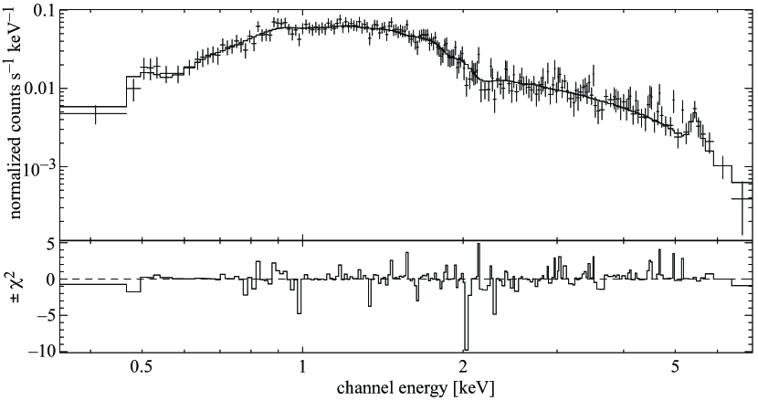
Figure 6: Chandra ACIS-I X-ray spectrum extracted in the central 78 arcsec ($280h_{70}^{-1}\,$kpc) superposed with a mekal plasma spectrum. Top: fit with $N_{\rm H}$ free. Bottom: the residuals are shown expressed as the $\chi^{2}$ contribution of each binned energy channel.

Table 1 summarizes the spectral fitting results. The best fit temperature, $kT$, varies between 5.3 and 5.6 keV depending on the free and fixed parameters, with an error bar of about 0.4 keV at $1\sigma$ confidence level. The metallicity, independently of parameters kept fixed, is $0.33Z_{\odot}$, with an error bar $0.09Z_{\odot}$ at $1\sigma$ confidence level. When we left the hydrogen column density free, we obtain $N_{\rm H}=(3.9\pm 1.2)\times 10^{20}$ cm^-2 which agrees, within less than $2\sigma$ error bars, with the Galactic value, $N_{\rm H}=(2.61\pm 0.07)\times 10^{20}$ cm^-2 given by the Leiden-Argentina-Bonn Survey (Kalberla et al. 2005).

Table 1: Results of the X-ray spectral fits in a circular region of radius 78 arcsec around the centre. “dof” is short for degrees of freedom.

$N_{\rm H}[10^{20}$cm-2]	$kT$ [keV]	$Z[Z_{\odot}]$	redshift	$\chi^{2}/$dof
$3.9\pm 1.2$	$5.3\pm 0.4$	$0.33\pm 0.09$	0.225	196.2/231
2.61	$5.6\pm 0.3$	$0.33\pm 0.09$	0.225	196.7/232
$3.9\pm 1.2$	$5.3\pm 0.4$	$0.33\pm 0.09$	$0.222\pm 0.007$	196.3/230

Note: Error bars are $1\sigma$ confidence level. Values without error bars are kept fixed.

We have also used the vmekal model, where the individual metal abundances are fitted independently. The results are presented in Table 2.

Table 2: Results of X-ray spectral fits with varying metal abundances. The error bars are $1\sigma$ confidence level. Temperature is in keV and the abundances in solar units.

O	Mg	Si	Ca	Fe	Ni
$0.9_{-0.9}^{+1.1}$	$1.9\pm 1.1$	$0.5\pm 0.5$	$2.2\pm 2.1$	$0.36\pm 0.09$	$2.7\pm 2.5$
$kT=5.4\pm 0.3$ keV			$\displaystyle{\frac{\chi^{2}}{\rm dof}=\frac{192.3}{227}}$

There is a marginal evidence of an over-abundance of $\alpha$-elements, mainly Mg (considering the error bars). The best fit value for Ni is also very high, 7.5 times the Fe abundance but, again, error bars prevent us from discussing further this question. We only present the individual metal abundances for completeness.

4.2 Radial profiles

4.2.1 Temperature profile

The radial temperature profile was obtained in concentric circular annuli where, for each annulus, a spectrum was extracted and fitted following the method described above, except that the hydrogen column density was kept fixed at the mean best-fit value found inside 78 arcsec (i.e., $N_{\rm H}=3.9\times 10^{20}$cm^-2). The annuli are defined by approximately the same number of counts (1000 counts, background corrected), so that the signal-to-noise in each annulus spectrum is roughly constant. Fig. 7 shows the temperature profile.

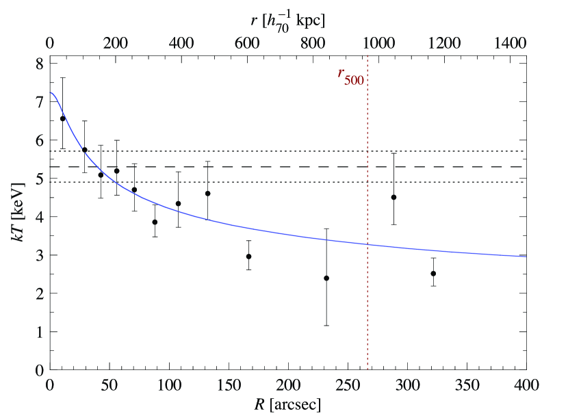
Figure 7: Temperature profile. The error bars are $1\sigma$ confidence level. The horizontal dashed line is the mean temperature inside 78 arcsec, $kT=5.3\pm 0.4$ keV, the horizontal dotted lines correspond to $1\sigma$ confidence level of the mean temperature. The continuous curve is the best-fit polytrope temperature profile. The vertical line shows $r_{500}$.

The temperature profile shown in Fig. 7 presents a visible gradient outwards. We therefore used a simple analytical temperature profile, described by a polytropic equation of state, to fit the observed data points. Although it is not clear if the ICM gas temperature is well described by a polytropic equation of state, some observations suggest that a polytrope with index $1.1\ga\gamma\la 1.3$ may be empirically used to describe the temperature radial profile (e.g. Markevitch et al. 1999; Lima Neto et al. 2003; Cypriano et al. 2005).

The use of a polytropic temperature profile has also the benefit of being easily deprojected. Thus, we have fitted a temperature profile given by:

$$T(r)=T_{0}\left[1+\left(\frac{r}{r_{c}}\right)^{2}\right]^{-3\beta(\gamma-1)/2}\,,$$ (1)

which is the temperature of a polytropic gas that follows a $\beta$-model radial profile. Here, $r_{c}$ and $\beta$ are the values obtained with the $\beta$-model fitting of the brightness surface profile (see Sect. 4.2.2 below), and $T_{0}$ is the central temperature. Notice that only $\gamma$ and $T_{0}$ are free parameters.

A standard least-square fit of Eq. (1) results in $T_{0}=7.2\pm 0.6$ keV and $\gamma=1.23\pm 0.04$, with a reduced $\chi^{2}=1.1$; the best-fit polytropic temperature profile is ploted in Fig. 7. The fitted polytropic index is below $5/3$, the value of an ideal gas, suggesting that the gas may be indeed in adiabatic equilibrium (see, eg., Sarazin 1988, Sect. 5.2).

4.2.2 X-ray brightness profile

The X-ray brightness profile of Abell 1942 was obtained with the task ellipse from STSDAS/IRAF. The image we have used was in the [0.3–7.0 keV], corrected by the exposure map and binned so that each image pixel has 2 arcsec. Prior to the ellipse fitting, the CCDs gaps and source points were masked. The brightness profile, shown in Fig. 8, could be measured up to $\sim 350$ arcsec ($1.26\,h_{70}^{-1}$Mpc) from the cluster centre.

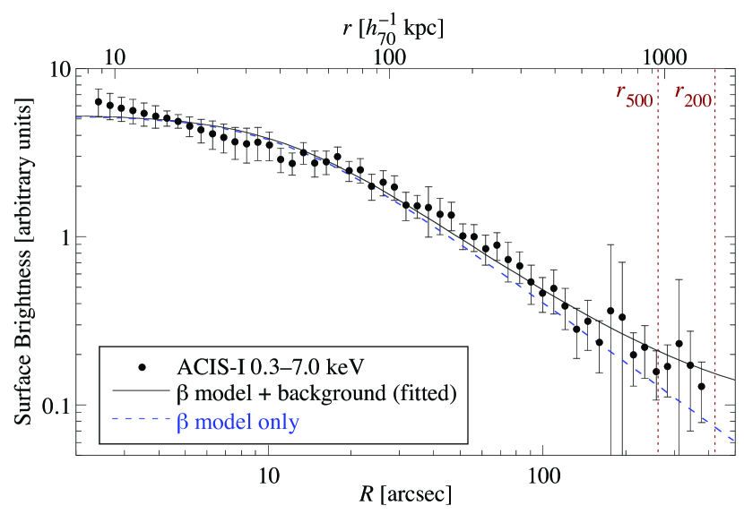
Figure 8: X-ray brightness profile. The full line shows the actual fit of a $\beta$-model plus a constant background, with $\beta=0.38\pm 0.01$ and $rc=12.5\pm 1.6\,$arcsec. The dashed line shows only the cluster contribution to the brightness profile. The vertical lines show $r_{200}$ and $r_{500}$ (see below).

In order to describe the surface brightness radial profile, we use the $\beta$-model (Cavaliere & Fusco-Femiano 1976):

$$\Sigma_{X}(R)=\Sigma_{0}\left[1+\left(\frac{R}{R_{c}}\right)^{2}\right]^{-3\beta+1/2}+\mbox{background}\,,$$ (2)

where we have added a constant to take into account the contribution of the background (both cosmic and particle). A least-squares fitting gives $\beta=0.38\pm 0.01$ and $R_{c}=12.5\pm 1.6$ arcsec ($45\pm 6\,h_{70}^{-1}$kpc). If we assume that the gas is approximately isothermal and distributed with spherical symmetry, there is a simple relation between the brightness profile and the gas number density, $n(r)$, i.e.,

$$n(r)=n_{0}\left[1+\left(\frac{r}{r_{c}}\right)^{2}\right]^{-3\beta/2}\,,$$ (3)

where $R_{c}=r_{c}$ (capital indicates projected 2D coordinates, lower case indicates 3D coordinates).

In order to estimate the central density, $n_{0}$, which is related to $\Sigma_{0}$, we integrate the bremsstrahlung emissivity along the line-of-sight in the central region. The result was compared with the flux obtained by spectral fitting of the same region, the normalization parameter of the thermal spectral model in xspec. This parameter, in turn, is proportional to $n_{e}n_{\rm H}\approx 1.2\,n_{\rm H}^{2}(r)$ (where $n_{e}$ and $n_{\rm H}$ are the electron and proton number densities, respectively). We obtain thus $n_{0}=(8.8\pm 0.9)\times 10^{-3}\,$cm^-3 (we drop the index H hereafter).

Abell 1942 presents a rather steep surface brightness profile (see Fig. 8). Such a profile is usually associated with a relaxed cluster with a cool-core, a drop in temperature of a factor $\sim 3$ in the centre compared to the maximum temperature.

However, we note that this cluster does not present any sign of a cool-core in the central part, at $r\approx 100\,h_{70}^{-1}\,$kpc, the smallest radius where we can extract a meaningful spectrum and measure the temperature. We actually measure an increase of the temperature from $r\approx 300\,h_{70}^{-1}\,$kpc towards the centre. We may be failing to detect a cool-core either because we lack the necessary spatial resolution or the intracluster gas is not cooling due to some physical heating process – as is the case of numerous clusters (e.g., Arnaud et al. 2005; Snowden et al. 2008).

Heating by cluster merging may be a possible mechanism. There is indeed a substructure at 1.7 arcmin towards the southeast from the cluster centre (see Fig.5). However, we may be simply not detecting an eventual drop in temperature because we lack the resolution. Using a sample of 20 clusters, Kaastra et al. (2004) show that the radius ($r_{c}$ in their paper) where the temperature drops in cooling-flow clusters is, with 2 exceptions, smaller than $70\,h_{70}^{-1}\,$kpc.

4.2.3 Mass profile

We compute the gas mass simply by integrating the density given by Eq. (3), assuming spherical symmetry which, in this case, seems a good approximation when we exclude the substructure at the southeast (see Fig. 5). The growth gas mass profile is shown in Fig. 9.

The total mass (“X-ray dynamical mass”) is estimated assuming either an isothermal temperature equal to the emission weighted mean temperature of the cluster, or the deprojected polytropic temperature radial profile fitted in Sect. 4.2.1. Assuming hydrostatic equilibrium and spherical symmetry, the corresponding dynamical mass for the $\beta$-model is shown in Fig. 9. The values for the $r_{200}$ and $r_{500}$ radii derived from this model are, respectively, $1.53\,h_{70}^{-1}\,$Mpc and $0.97\,h_{70}^{-1}\,$Mpc.

The difference in the dynamical mass estimates using the isothermal and polytropic temperature profiles are quite small. For the polytropic model, the mass profile rises more steeply near the center and than has a slower growth beyond $r\sim 300h_{70}^{-1}\,$kpc.

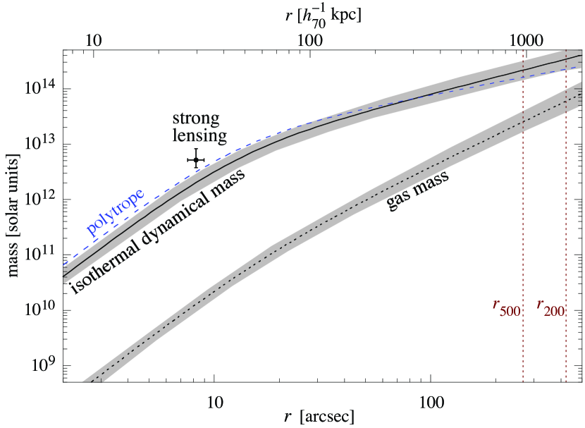
Figure 9: X-ray dynamical mass profiles and gas mass profile (dotted line). The full line corresponds to the dynamical mass computed assuming an isothermal $\beta$-model; the dashed line is corresponds to the polytropic temperature profile. The vertical lines correspond to $r_{200}$ and $r_{500}$. The grey shaded areas correspond to $1\sigma$ confidence level error bars. The single point named “strong lensing” is our estimate based on the position of the arc seen in Fig. 2 (see text for details).

We have also estimated the total mass using the gravitational arc shown in Fig. 2, discovered by Smail et al. (1991) assuming that this strong arc is located at the Einstein radius, $R_{E}$. Measuring the distance from the centre of the dominant galaxy, we have $R_{E}=8.2\pm 0.8$ arcsec or, at $z=0.225$, $R_{E}=(29.6\pm 2.9)h_{70}^{-1}\,$kpc. We then suppose, for simplicity, that the dynamical mass may be modelled by a singular isothermal sphere. If the background lensed galaxy is located between $0.6<z<4.0$ then the total mass inside $R_{E}$ is within $(3.6<M<8.0)\times 10^{12}\,M_{\odot}$. We show this mass estimate in Fig. 9, in comparison with the dynamical mass derived with X-ray data.

The gravitational lensing mass is about a factor 2 larger than the mass obtained with X-ray data, but the difference is only significant at less than $2\sigma$ confidence level. Indeed, this kind of situation, where the “lensing mass” is larger than “X-ray mass” is known for some time (Cypriano et al. 2004, e.g.). While the dynamical mass estimated by lensing effects may overestimate the total mass by including all contributing mass along the line-of-view, X-ray data derived masses may sometimes under-estimate the total mass, as shown by numerical simulations by Rasia et al. (2006).

5 Analysis of the Velocity Distribution

5.1 Kinematical Structures

We used the ROSTAT routines (Beers et al. 1990) to analyze the velocity distribution of the spectroscopic sample given in Table A.1. We identified the kinematical structures using the method of the weighted gap analysis, as discussed in Ribeiro et al. (2003). A weighted gap is defined by $y_{i}=(w_{i}g_{i})^{-1/2}\,,$ where the $g_{i}{\rm{}^{\prime}s}$ are the measured gaps between the ordered velocities, and the $w_{i}{\rm{}^{\prime}s}$ are a set of approximately Gaussian weights. A gap is considered significant if its value is greater than 2.25 (Wainer & Thissen 1976). The presence of big gaps in the velocity distribution indicates that we are not sampling a single structure. Fig. 10 (a) shows the redshift histogram for the entire spectroscopic sample where we have marked the main kinematical structures, defined as those having 3 or more members, found from the ROSTAT gap analysis.

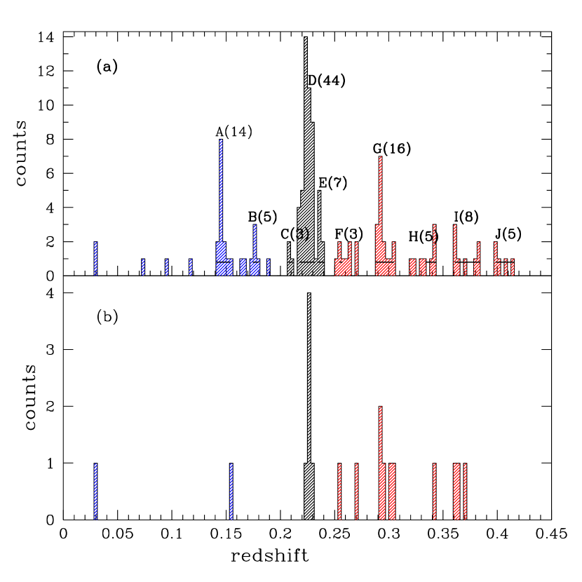
Figure 10: Upper panel: Histogram of the redshift distribution of our spectroscopic sample. Letters identify the kinematical structures found with the gap analysis The number of identified members are in parentheses. The horizontal lines inside the histograms of groups give the range of the groups as determined from the gap analysis. Lower panel: redshift distribution for the circular region enclosing the DC region.

The dominating kinematical structure labelled D, at redshift $\sim 0.22$, is (kinematically) centered on the brightest galaxy of the cluster A1942 (#067 in Table A.1; z = 0.225). It neighbours structures C and E which, given the relatively small redshifts distances ($\rm\Delta z\sim 0.012$), may, together with structure D, belong to a same superstructure. A new gap analysis using this subsample finds the same gaps as the previous analysis, indicating that these structures are indeed kinematically distinct from each other.

Using the sample of 44 redshifts belonging to structure D, which we may identify with the cluster A1942, we may obtain the cluster mean recessional velocity, $\overline{cz}=67493_{-249}^{+226}\leavevmode\nobreak\ \ {\rm km\,s^{-1}}$, which corresponds to the redshift $z_{A1942}=z_{D}=0.22513$ . For comparison, the recessional velocity of the brightest galaxy of the cluster is $67402\leavevmode\nobreak\ \ {\rm km\,s^{-1}}$. The cluster velocity dispersion corrected following Danese et al. (1980) is found to be $\sigma_{corr}=908_{-139}^{+147}\leavevmode\nobreak\ \ {\rm km\,s^{-1}}$. We notice that all the normality tests included in the ROSTAT package fail to reject the null hypothesis of a Gaussian distribution for this sample. The neighbours kinematical structures $C$ and $E$ are located at $z_{C}=0.20938$ and $z_{E}=0.23588$.

Fig. 11 shows the projected distribution of the galaxies corresponding to the kinematical structures discussed above. Notice that galaxies belonging to structures C, D and E seem to populate the same regions in projection, corroborating the suggestion that they are part of a bigger superstructure. The plot also suggests that the main structure D, which is the cluster A1942 itself, extends into a large region, maybe even larger than the one covered by our observations.

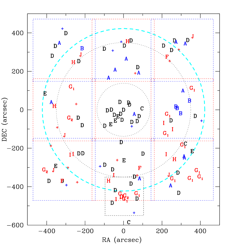
Figure 11: The projected distribution of the spectroscopic sample galaxies (Table A.1). Positions are given as offsets from the brightest A1942 galaxy, (#067 of Table A.1). Galaxies are labelled according to the kinematical structures they belong, given in Fig. 10 (a), whereas the crosses correspond to galaxies not assigned to any of them. The dotted lines are the boundaries of the EFOSC fields (Section 3), with the most southern one centered at the position of the “dark clump” suggested by Erben et al. (2000). The dashed circle of radius $r_{200}=1.53\,h_{70}^{-1}\leavevmode\nobreak\ \rm{Mpc}$ ($\sim 420\leavevmode\nobreak\ \rm{arcsec}$) show the limits of the virialized cluster. The dotted circles have radii $0.5\,h_{70}^{-1}\rm{Mpc}$ ($\sim 138\leavevmode\nobreak\ \rm{arcsec}$ ) and $1.26\,h_{70}^{-1}\rm{Mpc}$ ($\sim 350\leavevmode\nobreak\ \rm{arcsec}$, roughly corresponding to the region of X-ray emission).

The wedge diagrams of galaxies in right ascension and declination are displayed in Fig. 12. Both show the cluster and all galaxies collected in a square of 14.5 arcmin around the cluster centre. The main fore and background concentrations of Fig. 10(a), respectively $A$ and $G$ of Fig. 10(a) are clearly seen in this figure.

Figure 12: Wedge velocity diagram in right ascension (top), and declination (bottom) for the galaxies in the Abell 1942 field.

Fig. 13 shows the peculiar velocity distribution, $v_{pec}=c(z-z_{D})/(1+z_{D})$ of this sample. There are 3 galaxies belonging to the “E” group which are at the position corresponding to the X-ray substructure at $1.7\leavevmode\nobreak\ \rm{arcmin}$ towards the southeast from the cluster centre (see Section 4). In any case, we cannot conclude of a heating process of A1942 by a merging background group.

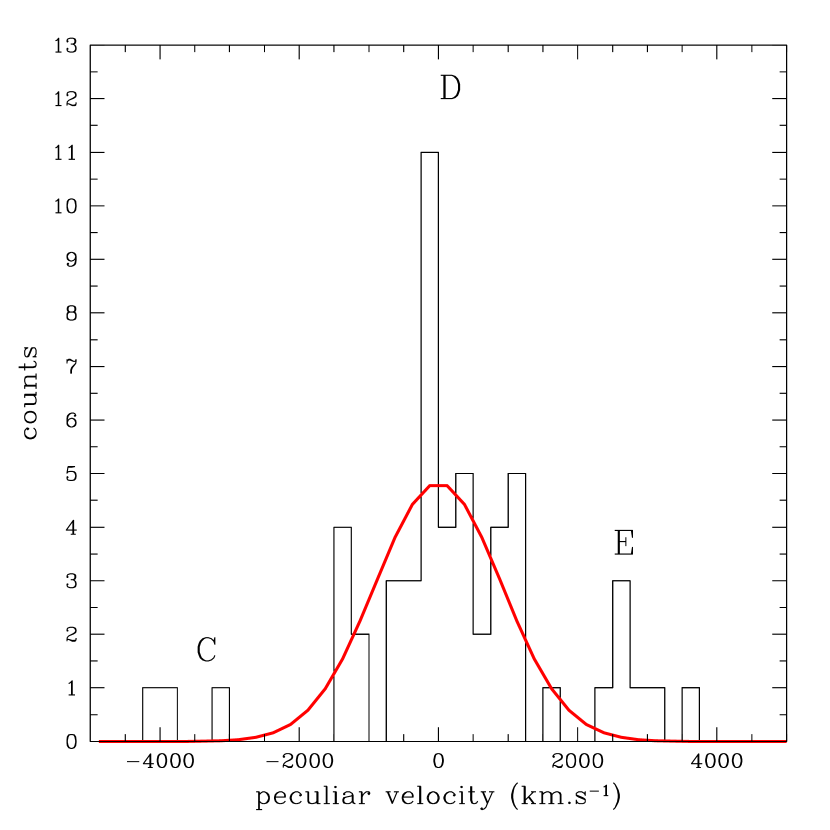
Figure 13: Peculiar velocity distribution in the interval comprising structures C, D and E. The continuous curve is a Gaussian with dispersion equal to that of structure D (section 5.1).

5.2 The dark clump

A massive dark clump (hereafter DC), with total mass equivalent to a rich cluster of galaxies and situated about 7 arcmin south to A1942 centre, was first suggested by Erben et al. (2000) based on a weak lensing signal detection made on high quality images obtained with the CFHT telescope. However, a more detailed study by von der Linden et al. (2006), using HST quality observations, confirmed the weak lensing signal detection but with much less significance. This finding, together with the fact that Chandra observations of the field did not showed any significant extended X-ray emission in the DC direction (Section 4), led the authors to scale down the total mass of the cluster by a factor of, at least, two as compared to the original value estimated by Erben et al. (2000), making unlikely the hypothesis of a dark matter halo of the size of a galaxy cluster. However, as the authors have pointed out, there is an noticeable excess of galaxies in this region, which is also apparent from the isopleths of the projected density of galaxies displayed in Fig. 3. Note that the projected density distribution nearby the DC region is elongated towards the same direction shown in the mass density maps produced by von der Linden et al. (2006) (see figure 9 of their paper), although being much more extended than it was found there (the mass density enhancements found by von der Linden et al. (2006) are mostly concentrated inside the dashed circle delimiting the DC region).

We have spectroscopic data for 15 galaxies in the DC direction, most of them in the background relative to A1942 , as can be seen in Fig. 11. The redshift distribution of these galaxies is shown in panel (b) of Fig. 10. As it can be seen by comparing with panel (a), the DC redshift distribution may be decomposed into the same kinematical groups as for the rest of the field. Hence, the spectroscopic data indicate that, considering only galaxies in the cluster background, $z>z_{D}$, there are two main kinematical structures, namely $G$ and $I$, that may be contributing for the weak-lensing signal associated to the DC. However, as it can be seen in Fig. 11, these 2 structures are much more spatially extended than the DC region, and tend to populate the entire southern part of field, as, in fact, most of the background galaxies we measured.

Additional clues on possible matter condensations that may be contributing to the weak-lens signal in the direction of the DC can be obtained by looking at the distribution of photometric redshifts. As part of an ongoing project of estimating photometric redshifts for all galaxies brighter then $r=21$ in the SDSS/DR6 using a procedure called Locally Weighted Regression briefly described in the Appendix (see also Atkeson et al. 1997; Boris et al. 2007; Abdalla et al. 2008), we have produced our own estimates of photometric redshifts for the region of Fig. 1.

Fig. 14 show the distribution of photometric redshifts obtained with the LWR technique for galaxies belonging both to the DC region and to its complementary region within the $18\times 18$ arcsec field of Fig. 3. Besides the fact that the brightest galaxies tend to avoid the DC region (shaded histograms), for the fainter galaxies ($18^{\rm{mag}}<m_{r}<21^{\rm{mag}}$) it can be seen that, whereas the redshift distribution of the complementary DC field peaks for redshifts $\geq 0.3$ (bottom panel), within the DC region it extends almost uniformly in the interval $0.3<z_{LWR}<0.45$.

Figure 14: The distribution of photometric redshifts for galaxies projected: (a) in a 120 arcsec radius circle enclosing the DC region; (b) in its complementary region within the $18\times 18$ arcsec field of Fig. 3. Shaded histograms corresponds to the brighter sample of galaxies $15^{\rm mag}<m_{r}<18^{\rm mag}$ and thick lines histogram to the fainter sample $18^{\rm mag}<m_{r}<21^{\rm mag}$. Letters identify some of the kinematical structures found in Fig. 10(a).

In order to see if the differences between the redshifts distributions have some spatial counterparts, we show in Fig. 15 the surface density of galaxies normalized by their total number, for two subsamples of faint galaxies, selected accordingly to their photometric redshifts: galaxies with photometric redshifts in the interval $0.2<z_{LWR}<0.25$ (panel A), which in principle should have a greater probability to belong to cluster A1942; and galaxies with $0.3<z_{LWR}<0.45$ (panel B) which constitute the major fraction of galaxies projected in the DC region. Comparing these 2 panels, it appears that galaxies with higher redshifts seem to have a slightly higher probability to be found nearby the DC direction than galaxies in the low redshift interval. This suggests that the density excess seen by Erben et al. (2000) should be due to line-of-sight background structures. Note that galaxies at this redshift are too faint to be included in our spectroscopic sample. Nevertheless, this is a hint of another structure that may be contributing to the weak-lensing signal. In conclusion, our analysis suggests that the DC weak-lensing signal, if not a mere statistical fluctuation (von der Linden et al. 2006), should probably be produced by several structures along the line-of-sight.

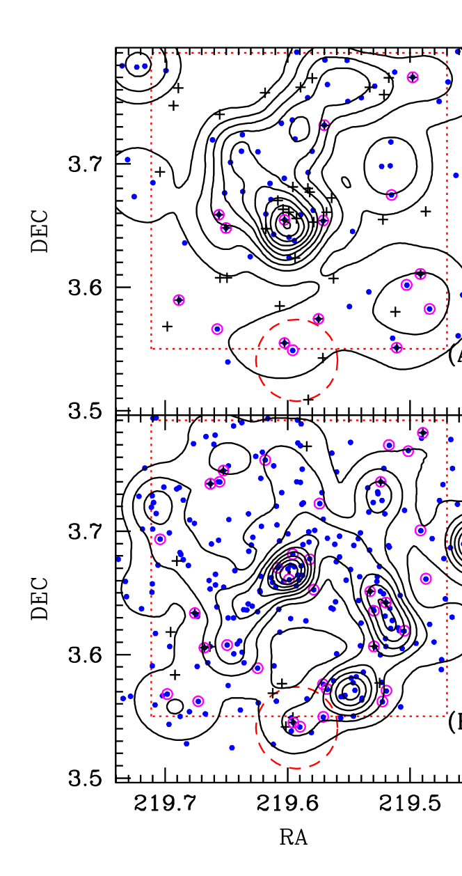
Figure 15: Contours of the surface probability density of galaxies for 2 subsamples of faint galaxies selected accordingly to their photometric redshift. Upper panel: $0.2<z_{LWR}<0.25$ ; lower panel: $0.3<z_{LWR}<0.45$. Filled circles show the positions of galaxies of the selected samples; those galaxies having a measured spectroscopic redshift are denoted by a large open circle. Galaxies from the spectroscopic sample having $z_{\rm spec}$ in the same interval defining the sample, are denoted by crosses. Contours are equally spaced by $\Delta_{\Sigma}=0.12$ with the highest level at $\Sigma_{Prob}^{max}=5\times 10^{-6}\,$arcsec^-2.

6 Summary and conclusion

We have investigated the cluster of galaxies Abell 1942. More than a hundred new spectroscopic redshifts were measured in a $14\times 14$ region around its centre. Together with X-ray archive data from Chandra, and photometric data from SDSS, we were able to achieve the dynamical and kinematical analysis of this cluster for the first time.

– We found that about half of the observed galaxies are kinematical members of the cluster. We have also found some kinematical evidence for the presence of nearby groups of galaxies whose spatial counterparts however have not been confirmed. The cluster is situated at redshift 0.22513.

– Our analysis indicates that inside a radius of $\sim 1.7h_{70}^{-1}\,$Mpc ($\sim 7\,$arcmin) the cluster galaxy distribution is well relaxed without any remarkable feature and with a mean velocity dispersion of $\sigma=908^{+147}_{-139}\ {\rm km\,s^{-1}}$.

– We have analyzed archival Chandra data and derived a mean temperature $kT=5.5\pm 0.5\,$keV and metal abundance $Z=0.33\pm 0.15Z_{\odot}$. The velocity dispersion corresponding to this temperature using the $T_{X}$–$\sigma$ scaling relation is in good agreement with the measured galaxies velocities. The X-ray emission traces fairly well the galaxy distribution.

– We derive dynamical mass estimates of the cluster, assuming hydrostatic equilibrium of the (isothermal) intracluster X-ray emitting gas. At a radius equivalent to $r_{500}$ we obtained $M_{\rm dyn}(<r_{500})\sim 5\times 10^{14}M_{\odot}$. An estimate of the dynamical mass using the gravitational arc found at about $\sim 8.2$ arcsec from the cluster centre showed it to be consistent with that derived from the hydrostatic equilibrium hypothesis.

– We do not confirm the mass concentration 7 arcmin south from the cluster centre from our dynamical and X-ray analysis. However, we do see a concentration of background galaxies towards these regions which may be at the origin of the weak lensing signal detected before.

Appendix A

Locally Weighted Regression (LWR) is a statistical method of a class known as memory-based learning. In this type of method, a training set remains stored until a result, an answer from a query, is obtained. LWR establishes a linear relationship between photometric feature vectors (magnitudes or colours and/or additional photometric parameters) and redshifts which is local because redshift estimation, at a given point in feature space, weighs more heavily the data points in the neighbourhood of this point than those more distant. For this work, we have used SDSS magnitudes (u, g, r, i, z) for the feature vectors. The training set contains feature vectors and spectroscopic redshifts for all objects and, from these values, we build a redshift estimator which is applied to the galaxies in the A1942 field.

For the training set, we have constructed a sample with 40951 unique galaxy spectroscopic redshifts, using a similar procedure described in Oyaizu et al. (2008). We selected randomly 20000 redshifts from SDSS-DR6 spectroscopic sample (Adelman-McCarthy et al. 2006), with confidence level $z_{conf}>0.9$. We also included the following unique galaxy redshifts from other surveys: 290 from CFRS (Canada-France Redshift Survey, Lilly et al. (1995)), with $Class>1$; 229 from DEEP (Deep Extragalactic Evolutionary Probe, Davis et al. (2001)) with $q_{z}=$ A or B; 6,245 from DEEP2 (Weiner et al. 2005) with $z_{quality}\geq 3$; 414 from CNOC2 (Canadian Network for Observational Cosmology Field Galaxy Survey, Yee et al. (2000)); 13,257 from 2SLAQ (2dF-SDSS LRG and QSO Survey, Cannon et al. (2006)) with $z_{op}\geq 3$; and 416 from TKRS (Team Keck Redshift Survey, Wirth et al. (2004)) with $z_{quality}>1$.

We have tested the method by comparing the photometric redshifts with the measured spectroscopic ones (described in Section 3). These results are quoted in Table A.1. Using a sigma-clipping procedure in order to exclude catastrophic outliers ($\sim 5\%$ of the sample) we found a rms dispersion of 0.097 between $z_{phot}$ and $z_{spec}$.

Table 3: Positions, photometric data, photometric and spectroscopic redshifts for galaxies of Abell 1942.

Gal.	R.A.	Decl	$u$	$g$	$r$	$i$	$z$	$z_{phot}$	error	$z_{spec}$	error	notes
	(2000)	(2000)						(LWR)
1	14 37 54.75	+03 39 15.7	22.301	20.283	19.315	18.907	18.610	0.088	0.052	0.16488	0.00032	em: $H\beta$,2OIII
2	14 37 55.18	+03 34 22.7	22.875	22.012	20.747	20.191	19.755	0.459	0.075	0.29303	0.00014	R: 4.85
3	14 37 56.19	+03 34 54.9	25.629	21.395	19.982	19.437	18.886	0.221	0.047	0.29046	0.00018	R: 5.04
4	14 37 56.94	+03 39 41.9	22.573	21.417	19.943	19.406	19.069	0.350	0.057	0.22980	0.00028	R: 3.02
5	14 37 57.52	+03 46 50.9	23.519	22.251	20.674	20.148	19.854	0.339	0.072	0.39893	0.00012	em: OII
6	14 37 57.98	+03 42 03.4	20.923	20.545	19.734	19.428	19.128	0.415	0.057	0.29414	0.00010	em: OII
7	14 37 58.00	+03 36 38.2	22.116	20.677	19.533	19.059	18.812	0.249	0.077	0.24038	0.00018	R: 3.04
8	14 37 58.58	+03 34 14.6	21.339	20.364	19.499	19.272	19.138	0.269	0.048	0.29027	0.00032	R: 3.12 very weak
9	14 37 58.93	+03 41 01.5	20.440	19.154	18.370	17.979	17.697	0.161	0.038	0.17489	0.00015	R: 6.12
10	14 37 59.55	+03 46 16.2	22.249	20.199	18.866	18.369	18.097	0.242	0.039	0.22297	0.00012	R: 8.47
11	14 38 00.38	+03 37 17.2	23.322	21.762	21.536	21.339	21.695			0.20759	0.00016	R: 3.37
12	14 38 00.42	+03 45 56.6	25.051	20.510	19.558	19.074	18.817	0.325	0.047	0.14665	0.00019	R: 3.67
13	14 38 00.71	+03 36 05.4	21.946	22.071	19.872	19.780	19.128	0.216	0.042	0.14199	0.00019	R: 3.02
14	14 38 00.83	+03 36 12.5	21.851	19.601	18.663	18.245	17.891	0.096	0.024	0.14403	0.00056	em: OII,$H\beta$,2OIII
15	14 38 01.17	+03 37 08.4	21.853	19.828	18.205	17.659	17.301	0.303	0.023	0.29125	0.00016	R: 5.82
16	14 38 01.21	+03 41 54.4	19.853	18.450	17.615	17.193	16.917	0.142	0.027	0.14915	0.00016	R: 4.90 em: OII $z$=0.15048
										0.15006		SDSS
17	14 38 02.00	+03 39 55.6	21.189	20.104	19.564	19.276	19.145	0.134	0.042	0.17558	0.00013	em: $H\beta$,2OIII
18	14 38 02.48	+03 45 26.4	22.480	20.698	22.549	19.353	19.569			0.26529	0.00038	R: 3.09
19	14 38 02.66	+03 33 01.2	23.727	20.840	19.613	19.158	18.871	0.231	0.055	0.22390	0.00013	R: 3.08
20	14 38 02.96	+03 34 46.5	21.334	19.434	18.194	17.724	17.519	0.196	0.023	0.22483	0.00008	R: 10.67
21	14 38 03.21	+03 40 22.3	20.371	19.098	18.264	17.662	17.352	0.156	0.036	0.17596	0.00014	R: 3.62
										0.17548	0.00043	em: OII,$H\beta$,2OIII
22	14 38 03.62	+03 46 07.7	20.601	19.248	18.463	18.034	17.765	0.138	0.042	0.14806	0.00021	R: 3.61
23	14 38 03.68	+03 40 30.3	21.757	20.351	19.766	19.501	19.698	0.201	0.046	0.17642	0.00021	em: OII,$H\beta$,2OIII
24	14 38 04.17	+03 35 56.5	22.681	21.958	21.090	20.874	21.121	0.342	0.098	0.33790	0.00014	em: OII very weak
25	14 38 04.20	+03 46 14.7	22.609	21.378	20.237	19.729	19.337	0.385	0.077	0.22394	0.00025	R: 3.03
26	14 38 04.68	+03 34 12.7	22.362	21.003	19.625	19.110	18.755	0.318	0.059	0.29304	0.00014	R: 4.68
27	14 38 04.80	+03 38 31.5	23.483	22.528	20.851	20.272	19.915	0.436	0.064	0.36106	0.00019	R: 3.11
28	14 38 05.18	+03 45 24.4	23.857	20.491	19.257	18.727	18.261	0.177	0.038	0.22919	0.00019	R: 4.13
29	14 38 05.37	+03 39 17.9	22.576	21.189	19.989	19.554	19.158	0.293	0.087	0.22980	0.00028	R: 3.02 weak
30	14 38 05.49	+03 33 40.5	21.891	20.160	19.317	18.912	18.602	0.352	0.065	0.14504	0.00022	R: 4.75
31	14 38 05.82	+03 44 26.5	21.756	20.838	19.485	18.924	18.676	0.372	0.068	0.32107	0.00021	R: 3.48
32	14 38 06.03	+03 34 35.4	22.062	20.404	19.384	18.980	18.790	0.161	0.067	0.40309	0.00027	em: OII,$H\delta$,$H\beta$,2OIII
33	14 38 06.45	+03 39 47.6	22.943	21.288	19.747	19.217	18.856	0.339	0.045	0.28833	0.00016	R: 4.18 em: OII $z$= 0.28834
34	14 38 06.80	+03 44 49.2	22.127	20.474	19.949	19.878	19.953			0.25692	0.00012	em: $H\beta$
35	14 38 07.13	+03 36 23.2	23.965	22.246	20.588	20.044	19.473	0.390	0.045	0.37891	0.00021	R: 4.18
36	14 38 07.13	+03 38 07.4	24.399	22.260	20.468	20.043	19.768	0.406	0.044	0.29209	0.00035	R: 2.63 very weak
37	14 38 07.86	+03 39 04.8	21.160	19.789	18.216	17.651	17.293	0.302	0.026	0.36109	0.00019	R: 3.65
38	14 38 07.97	+03 45 46.6	21.026	20.384	19.762	19.427	19.600	0.295	0.047	0.22180	0.00014	em: OII
39	14 38 15.12	+03 36 25.3	21.255	20.318	19.765	19.584	19.227	0.181	0.043	0.23002	0.00013	em: OII
40	14 38 15.42	+03 40 20.9	23.061	21.657	20.284	19.837	19.607	0.265	0.080	0.20869	0.00018	R: 3.04 very weak
41	14 38 16.24	+03 35 10.3	21.536	20.649	19.774	19.324	18.969	0.270	0.051	0.25485	0.00020	R: 3.09 very weak
42	14 38 16.41	+03 34 17.4	22.596	21.341	20.664	20.383	20.303	0.335	0.078	0.15343	0.00026	R: 3.01

Gal.	R.A.	Decl	$u$	$g$	$r$	$i$	$z$	$z_{phot}$	$error$	$z_{spec}$	error	notes
	(2000)	(2000)						(LWR)
43	14 38 16.46	+03 39 40.0	22.922	20.650	19.317	18.834	18.422	0.259	0.043	0.22237	0.00011	R: 7.46
44	14 38 16.58	+03 43 26.7	20.507	19.752	19.339	18.988	19.037	0.163	0.036	0.14155	0.00045	em: $H\beta$,2OIII
45	14 38 16.88	+03 43 54.9	21.584	19.492	18.152	17.668	17.398	0.235	0.022	0.21841	0.00013	R: 6.82
46	14 38 17.09	+03 39 14.5	24.485	20.968	19.739	19.263	19.063	0.228	0.040	0.22257	0.00021	R: 3.66
47	14 38 17.12	+03 32 55.4	22.234	21.133	20.213	19.818	19.823	0.313	0.062	0.29395	0.00021	R: 3.90
48	14 38 17.15	+03 34 32.0	22.210	21.069	19.866	19.263	18.889	0.407	0.077	0.26918	0.00004	em: $H\beta$
49	14 38 17.16	+03 32 31.2	21.720	20.624	19.635	19.315	19.057	0.278	0.057	0.22896	0.00028	R: 3.28
50	14 38 17.83	+03 43 23.2	23.431	21.609	20.348	19.810	19.302	0.352	0.070	0.26016	0.00017	R: 3.04 weak
51	14 38 18.04	+03 34 25.5	22.301	20.024	18.659	18.178	17.800	0.240	0.029	0.22682	0.00009	R: 10.73
										0.22625	0.00013	R: 6.62
52	14 38 18.12	+03 39 52.4	22.875	20.492	19.459	19.136	18.893	0.123	0.054	0.15097	0.00019	R: 3.04
53	14 38 18.20	+03 31 17.7	17.311	15.965	15.362	15.047	14.814	0.039	0.016	0.02899	0.00020	em: $H\beta$,$H\alpha$,SI
										0.02877		SDSS
54	14 38 18.93	+03 38 22.5	23.251	22.207	21.814	21.666	21.927	0.681	0.192	0.02816	0.00006	em: $H\alpha$,NII
										0.02802		SDSS
55	14 38 18.97	+03 39 09.8	22.256	20.970	19.718	19.227	18.844	0.321	0.081	0.22833	0.00015	R: 5.54
56	14 38 19.23	+03 46 13.9	22.991	20.532	19.203	18.692	18.329	0.270	0.038	0.22880	0.00013	R: 6.42
57	14 38 19.27	+03 33 49.3	20.389	18.982	17.694	17.256	16.943	0.235	0.031	0.22719	0.00011	R: 5.27
										0.22625	0.00031	R: 3.08
58	14 38 19.76	+03 40 39.1	22.874	21.837	20.579	20.031	19.806	0.384	0.073	0.22383	0.00019	R: 3.05
59	14 38 20.02	+03 30 27.9	21.294	20.017	19.247	18.872	18.719	0.157	0.053	0.21106		uncertain
60	14 38 20.09	+03 40 50.2	22.755	20.676	19.276	18.784	18.420	0.268	0.061	0.22985	0.00033	R: 3.09
61	14 38 20.41	+03 46 10.4	22.100	21.369	20.538	20.746	20.110	0.296	0.080	0.34347	0.00009	em: OII
62	14 38 20.96	+03 44 39.8	19.853	18.004	16.937	16.511	16.140	0.138	0.011	0.14667	0.00010	R: 7.71
										0.14688		SDSS
63	14 38 21.47	+03 32 43.8	23.094	21.450	21.075	21.075	21.220	0.131	0.105	0.30440	0.00012	em: OII
64	14 38 21.59	+03 45 47.3	21.247	19.623	18.316	17.857	17.495	0.261	0.028	0.22408	0.00010	R: 8.12
65	14 38 21.63	+03 35 51.1	22.705	21.938	21.277	20.982	20.928	0.359	0.104	0.23596	0.00026	R: 3.03
66	14 38 21.67	+03 32 27.2	23.958	21.441	20.062	19.457	19.171	0.354	0.037	0.29285	0.00021	R: 4.65
67	14 38 21.85	+03 40 12.9	19.720	17.557	16.226	15.698	15.331	0.168	0.015	0.22483	0.00025	R: 5.55
										0.22475		SDSS
68	14 38 22.39	+03 39 21.3	22.314	21.480	20.161	19.685	19.390	0.410	0.095	0.22662	0.00044	R: 3.01 weak
										0.22573	0.00029	R: 3.01 weak
69	14 38 22.55	+03 32 36.8	23.520	21.309	20.153	19.598	19.307	0.260	0.064	0.29351	0.00019	R: 3.22
70	14 38 22.63	+03 37 25.3	21.054	19.479	18.418	18.027	17.748	0.196	0.036	0.21867	0.00021	R: 3.02
71	14 38 22.64	+03 46 07.4	20.394	19.406	18.722	18.370	18.211	0.195	0.035	0.16666	0.00033	R: 3.19
												em:OII,$H\beta$,2OIII $z$=0.16471
72	14 38 22.84	+03 39 51.8	21.552	19.317	17.966	17.468	17.138	0.230	0.017	0.22109	0.00012	R: 8.56
73	14 38 22.98	+03 32 39.3	22.065	21.421	20.172	19.629	19.316	0.434	0.065	0.36555	0.00010	R: 3.03
74	14 38 23.13	+03 40 53.6	22.720	20.210	18.869	18.387	18.051	0.318	0.031	0.23017	0.00024	R: 3.62
75	14 38 23.15	+03 32 53.9	20.972	19.839	19.074	18.676	18.454	0.211	0.039	0.30181	0.00023	R: 3.02 em: $z$= 0.30277
										0.30318	0.00017	R: 5.12
76	14 38 23.83	+03 39 39.4	21.773	20.782	19.589	19.115	18.804	0.380	0.079	0.23579	0.00013	R: 6.69

Gal.	R.A.	Decl	$u$	$g$	$r$	$i$	$z$	$z_{phot}$	$error$	$z_{spec}$	error	notes
	$(2000)$	$(2000)$						(LWR)
77	14 38 24.19	+03 35 48.2	22.968	21.574	20.381	19.920	19.623	0.269	0.080	0.26374	0.00023	uncertain
78	14 38 24.43	+03 32 26.8	21.937	20.926	20.256	20.192	19.883	0.136	0.065	0.36131	0.00025	R: 3.04
79	14 38 24.73	+03 33 14.6	22.114	20.126	18.846	18.340	17.986	0.220	0.039	0.22586	0.00008	R: 10.74
										0.22608	0.00010	R: 8.15
80	14 38 24.73	+03 39 17.3	22.317	20.532	19.251	18.779	18.488	0.231	0.053	0.23644	0.00013	R: 6.53
81	14 38 24.80	+03 43 42.9	20.938	18.910	17.809	17.331	16.989	0.165	0.015	0.14675	0.00012	R: 6.85
82	14 38 25.04	+03 39 47.5	20.779	19.689	18.901	18.609	18.472	0.193	0.040	0.21830	0.00038	R: 3.15
83	14 38 25.27	+03 34 33.1	22.222	21.431	20.966	20.740	20.422	0.272	0.098	0.37008		em: OII
84	14 38 25.60	+03 45 20.7	19.274	18.234	17.928	17.680	17.566	0.053	0.027	0.07448	0.00011	em: OII,$H\beta$,2OIII
85	14 38 25.67	+03 35 03.9	21.409	19.570	18.541	18.120	17.821	0.137	0.035	0.22499	0.00010	R: 8.59
										0.22524	0.00010	R: 8.15
86	14 38 26.03	+03 40 14.1	22.982	21.885	20.461	20.038	19.848	0.333	0.065	0.21985	0.00016	R: 3.02
87	14 38 25.80	+03 32 09.5	22.822	23.250	22.193	21.833	21.383	0.668	0.036	0.22622	0.00022	R: 3.01
88	14 38 26.30	+03 38 58.5	21.026	18.472	17.052	16.540	16.232	0.241	0.017	0.23593	0.00019	R: 5.05
										0.23549		SDSS
89	14 38 27.03	+03 43 01.2	19.550	17.503	16.405	15.977	15.635	0.144	0.014	0.14532	0.00017	R: 4.06
										0.14621		SDSS
90	14 38 27.09	+03 34 04.5	23.120	20.514	19.461	19.071	18.641	0.092	0.045	0.34219	0.00050	weak
										0.33940	0.00050	weak
91	14 38 27.37	+03 40 07.1	25.064	22.839	21.524	21.082	20.670	0.553	0.047	0.22561	0.00024	R: 4.13
92	14 38 28.39	+03 38 50.5	22.461	20.825	19.470	18.997	18.683	0.260	0.058	0.22131	0.00015	R: 4.37
93	14 38 28.43	+03 35 25.6	24.400	22.198	21.362	20.886	20.815	0.449	0.065	0.22557	0.00019	R: 3.02 very weak
94	14 38 28.54	+03 45 30.8	23.794	23.036	20.741	20.093	19.901	0.403	0.044	0.23129		uncertain
95	14 38 30.00	+03 35 18.4	22.482	21.345	19.838	19.322	18.905	0.354	0.062	0.09505	0.00023	R: 3.10
96	14 38 35.98	+03 36 26.6	21.731	20.405	19.267	18.867	18.612	0.320	0.069	0.21806	0.00014	R: 6.40
97	14 38 36.21	+03 38 52.6	23.617	20.411	19.112	18.621	18.335	0.217	0.032	0.22678	0.00013	R: 5.99
98	14 38 36.30	+03 45 32.9	23.684	21.893	21.179	21.024	20.955	0.216	0.041	0.17978	0.00045	em: OII,$H\beta$,2OIII
99	14 38 36.73	+03 45 00.1	23.562	21.635	20.110	19.527	19.022	0.385	0.039	0.39874	0.00024	R: 3.57
100	14 38 37.40	+03 36 26.6	21.741	20.215	18.877	18.408	18.055	0.275	0.046	0.22483	0.00021	R: 4.01
101	14 38 37.47	+03 44 26.4	22.956	21.766	20.889	20.546	20.443	0.439	0.093	0.05753	0.22473	0.00021 R: 3.50
102	14 38 37.59	+03 39 31.9	21.825	19.670	18.394	17.880	17.530	0.231	0.024	0.02830	0.22427	0.00030 R: 4.12
103	14 38 37.98	+03 33 56.0	21.510	20.518	19.747	19.395	19.103	0.242	0.042	0.25180	0.00044	R: 3.04 weak
104	14 38 38.33	+03 40 43.4	22.905	19.760	18.606	18.110	17.679	0.059	0.028	0.62151	0.00024	em: OII
105	14 38 39.29	+03 44 20.9	21.654	21.366	20.396	20.120	19.559	0.300	0.078	0.33398	0.00015	em: OII
106	14 38 39.42	+03 36 22.1	21.334	21.310	20.142	19.736	19.408	0.451	0.055	0.38311	0.00022	em: OII very weak
107	14 38 39.91	+03 42 09.5	22.294	20.753	19.591	19.116	18.755	0.268	0.078	0.29289	0.00031	R: 2.60 very weak
108	14 38 40.46	+03 36 18.6	24.890	22.091	20.952	20.713	20.275	0.340	0.047	0.38371	0.00006	em: OII
109	14 38 40.52	+03 39 28.4	20.868	19.866	18.629	18.155	17.762	0.272	0.057	0.29957	0.00005	em: OII,2OIII
110	14 38 41.17	+03 35 13.1	22.309	21.852	21.153	20.822	20.640	0.538	0.098	0.32819	0.00011	em: OII
111	14 38 41.72	+03 33 41.4	22.291	22.062	20.516	20.044	19.596	0.381	0.063	0.18944	0.00018	R: 3.02
112	14 38 41.88	+03 46 52.5	21.558	19.208	17.751	17.233	16.821	0.248	0.018	0.22659	0.00011	R: 10.21
113	14 38 42.19	+03 34 15.8								0.25574	0.00026	em: OII,$H\beta$,2OIII ($\star$)
114	14 38 42.38	+03 38 00.8	22.408	20.115	18.991	18.422	17.938	0.340	0.038	0.40693		measured on H and K
115	14 38 43.13	+03 47 15.7	18.994	17.334	16.472	16.080	15.769	0.094	0.021	0.11659	0.00011	R: 9.50
										0.11633		SDSS

Gal.	R.A.	Decl	$u$	$g$	$r$	$i$	$z$	$z_{phot}$	$error$	$z_{spec}$	error	notes
	(2000)	(2000)						(LWR)
116	14 38 43.20	+03 34 02.6	20.200	19.075	17.956	17.445	17.172	0.210	0.041	0.22769	0.00018	R: 3.66
117	14 38 44.34	+03 46 02.7	22.847	21.024	19.962	19.585	19.747	0.023	0.082	0.14677	0.00024	R: 4.54
118	14 38 44.90	+03 38 41.6	20.823	19.396	18.763	18.474	18.399	0.081	0.042	0.26911	0.00070	uncertain
119	14 38 45.49	+03 35 20.7	21.925	21.059	20.466	20.170	19.895	0.239	0.075	0.23824	0.00030	em: OII,$H\beta$,2OIII
120	14 38 45.59	+03 45 45.1	23.102	21.756	20.684	20.139	20.187	0.674	0.084	0.22347	0.00022	R: 3.19
121	14 38 45.88	+03 40 33.4	21.710	20.690	19.764	19.369	18.973	0.271	0.038	0.34203	0.00026	R: 3.04 em: OII $z$= 0.34238
122	14 38 46.23	+03 34 59.1	25.929	22.260	20.808	20.204	19.685	0.574	0.047	0.41526	0.00020	R: 3.09 weak
123	14 38 46.60	+03 44 53.2	25.893	22.189	20.838	20.277	19.455	0.613	0.047	0.21933	0.00018	R: 3.01 very weak
124	14 38 46.99	+03 40 54.5	19.751	18.323	17.537	17.133	16.861	0.122	0.027	0.14636	0.00021	R: 3.09
										0.14675		SDSS
125	14 38 47.13	+03 37 04.4	21.057	21.050	20.447	20.451	20.669	0.148	0.107	0.32344	0.00012	em: OII
126	14 38 47.78	+03 34 02.7	24.408	21.495	20.163	19.775	19.359	0.311	0.047	0.22545	0.00016	R: 4.75
127	14 38 49.14	+03 41 37.7	22.913	21.242	19.542	18.985	18.646	0.354	0.036	0.23440	0.00006	em: $H\beta$
128	14 38 49.16	+03 34 58.6	22.195	21.919	21.093	20.786	20.297	0.490	0.091	0.30402	0.00032	R: 3.02 very weak

Note to Table A.1:
$\star$  galaxy # 113 is too faint: no photometric data found in SDSS database.