Implementing Communication-Optimal Parallel and Sequential QR Factorizations

Abstract

We present parallel and sequential dense QR factorization algorithms for tall and skinny matrices and general rectangular matrices that both minimize communication, and are as stable as Householder QR. The sequential and parallel algorithms for tall and skinny matrices lead to significant speedups in practice over some of the existing algorithms, including LAPACK and ScaLAPACK, for example up to 6.7x over ScaLAPACK. The parallel algorithm for general rectangular matrices is estimated to show significant speedups over ScaLAPACK, up to 22x over ScaLAPACK.

1 Introduction

In this paper we present parallel and sequential dense QR factorization algorithms that both minimize communication, and are as stable as Householder QR. (That is to say normwise backward stable.) Communication refers to messages that are sent over a network in the parallel case, and to data movement between different levels of memory hierarchy in the sequential case. The first set of algorithms, “Tall Skinny QR” (TSQR), are for matrices for which the number of rows is much larger than the number of columns, and which have their rows distributed over processors in a one-dimensional (1-D) block row layout. The second set of algorithms, “Communication-Avoiding QR” (CAQR), are for general rectangular matrices distributed using a two-dimensional (2-D) block cyclic layout. Some of these algorithms are new, and some are based on existing work.

The new algorithms are superior in both theory and practice. In [8] we show that the new sequential and parallel algorithms, for both 1-D layout TSQR and 2-D block cyclic layout CAQR, are communication optimal (modulo polylogarithmic factors), that is they are optimal in bandwidth and latency costs. This assumes $O(n^{3})$ algorithms (non-Strassen-like). We also observe in [8] that LAPACK’s corresponding sequential factorization and ScaLAPACK’s parallel QR factorization perform asymptotically more communication. The sequential recursive QR factorization algorithm by Elmroth and Gustavson [12] attains the lower bound on the volume of data transferred in some special cases, though not the lower bound on the number of block transfers.

In this paper, we focus on the implementation and performance results of these algorithms. The efficient implementation of the QR factorizations of tall and skinny matrices distributed in a 1-D layout is very important, since this operation arises in a wide range of applications. We cite three important examples. Block iterative methods frequently compute the QR factorization of a tall and skinny dense matrix. This includes algorithms for solving linear systems $Ax=B$ with multiple right-hand sides (such as variants of GMRES, QMR, or CG [34, 13, 26]), as well as block iterative eigensolvers (for a summary of such methods, see [3, 23]). Many of these methods have widely used implementations, on which a large community of scientists and engineers depends for their computational tasks. Examples include TRLAN (Thick Restart Lanczos), BLZPACK (Block Lanczos), Anasazi (various block methods), and PRIMME (block Jacobi-Davidson methods) [35, 24, 20, 2, 4, 31]. Eigenvalue computation is particularly sensitive to the accuracy of the orthogonalization; two recent papers suggest that large-scale eigenvalue applications require a stable QR factorization [19, 21]. Our approach is based on Householder reflections so it is unconditionnally normwise backward stable, as opposed to other standard used methods as Gram-Schmidt or CholeskyQR (see Section 5).

Recent research has reawakened an interest in alternate formulations of Krylov subspace methods, called $s$-step Krylov methods, in which some number $s$ steps of the algorithm are performed all at once, in order to reduce communication. Demmel et al. review the existing literature and discuss new advances in this area [10]. Such a method generates some basis for the Krylov subspace, and then a QR factorization is used to orthogonalize the basis vectors. This is an ideal application for TSQR, and in fact inspired its (re-)discovery.

Householder QR decompositions of tall and skinny matrices also comprise the panel factorization step for typical QR factorizations of matrices in a more general, two-dimensional layout. This includes the current parallel QR factorization routine PDGEQRF in ScaLAPACK, as well as ScaLAPACK’s out-of-DRAM QR factorization PFDGEQRF [7]. Both algorithms use a standard column-based Householder QR for the panel factorizations, but in the parallel case this is a latency bottleneck, and in the out-of-DRAM case it is a bandwidth bottleneck. Our CAQR algorithm for computing the QR factorization of general rectangular matrices uses TSQR for its panel factorization. That’s how CAQR removes the latency bottleneck in the parallel case and the bandwidth bottleneck in the sequential case.

The main insight behind TSQR algorithm is to perform the QR factorization of a tall-skinny matrix as a reduction operation. This idea itself is not novel (see for example, [1, 5, 6, 15, 18, 22, 27, 28, 29]), but we have a number of optimizations and generalizations:

• Our TSQR algorithm can compute most of its floating-point operations by using the best available sequential QR factorization. In particular, we can achieve significant speedups by invoking Elmroth and Gustavson’s recursive QR (see [11, 12]).

• We use TSQR as a building block for CAQR, the parallel factorization of rectangular matrices with a two-dimensional block cyclic layout. To our knowledge, parallel CAQR is a new algorithm.

• We explain how TSQR can work on general reduction trees. This flexibility lets schedulers overlap communication and computation, and minimize communication for more complicated and realistic computers with multiple levels of parallelism and memory hierarchy (e.g., a system with disk, DRAM, and cache on multiple boards each containing one or more multicore chips of different clock speeds, along with compute accelerator hardware like GPUs).

In practice, parallel TSQR leads to significant speedups on several machines:

• up to $6.7\times$ on 16 processors of a Pentium III cluster, for a $100,000\times 200$ matrix; and

• up to $4\times$ on 32 processors of a BlueGene/L, for a $1,000,000\times 50$ matrix.

Some of this speedup is enabled by TSQR being able to use a much better local QR decomposition than ScaLAPACK can use, such as the recursive variant by Elmroth and Gustavson [12]. We have also implemented sequential TSQR on a laptop for matrices that do not fit in DRAM, so that slow memory is disk. This requires a special implementation in order to run at all, since virtual memory does not accommodate matrices of the sizes we tried. By extrapolating runtime from matrices that do fit in DRAM, we can say that our out-of-DRAM implementation was as little as $2\times$ slower than the predicted runtime as though DRAM were infinite.

We also estimate the performance of our parallel CAQR algorithm (whose actual implementation and measurement is current work), yielding predicted speedups over ScaLAPACK’s PDGEQRF of up to $22.9\times$ on a model Petascale machine. The best speedups occur for the largest number of processors used, and for matrices that do not fill all of memory, since in this case latency costs dominate. In general, when the largest possible matrices are used, computation costs dominate the communication costs and improved communication does not help.

The rest of the paper is organized as follows. Section 2 describes the algebra of the TSQR algorithm and shows how the parallel and sequential versions correspond to different trees. Section 3 shows that the local QR decompositions in TSQR can be further optimized by exploiting the structure of the matrices involved. We also explain how to apply the $Q$ factor from TSQR efficiently, which is needed both for CAQR and other applications. Section 4 describes the parallel and sequential TSQR algorithms, and presents a performance model for each. Next, Section 5 describes other “tall skinny QR” algorithms, such as CholeskyQR and Gram-Schmidt, and compares their cost and numerical stability to that of TSQR. This section shows that TSQR is the only algorithm that simultaneously minimizes communication and is numerically stable. Section 6 describes the parallel CAQR algorithm and constructs a performance model. Section 7 presents the platforms used for testing, and discusses the TSQR and CAQR performance results. Section 8 concludes the paper.

2 TSQR matrix algebra

In this section, we illustrate the insight behind the TSQR algorithm for computing the QR factorization of an $m\times n$ matrix $A$ partitioned in $P$ block rows, that is $A=[A_{0};A_{1};\cdots;A_{P-1}]$. We use Matlab notation, so that the $A_{i}$ are stacked atop one another.

TSQR defines a family of algorithms, in which the QR factorization of $A$ is obtained by performing a sequence of QR factorizations until the lower trapezoidal part of $A$ is annihilated and the final $R$ factor is obtained. The QR factorizations are performed on block rows of $A$ and on previously obtained $R$ factors, stacked atop one another. We call the pattern followed during this sequence of QR factorizations a reduction tree. We begin with parallel TSQR, for which the reduction tree is a binary tree, and later show sequential TSQR on a linear tree. We consider the simple example of $P=4$.

Parallel TSQR starts with the independent computation of the QR factorization of each block row:

$$A=\begin{pmatrix}A_{0}\\ A_{1}\\ A_{2}\\ A_{3}\\ \end{pmatrix}=\begin{pmatrix}Q_{00}R_{00}\\ Q_{10}R_{10}\\ Q_{20}R_{20}\\ Q_{30}R_{30}\\ \end{pmatrix}.$$

This is “stage 0” of the computation, hence the second subscript 0 of the $Q$ and $R$ factors. The first subscript indicates the block index at that stage. Stage 0 operates on the $P=4$ leaves of the tree. After this stage, there are $P=4$ of the $R$ factors. We group them into successive pairs $R_{i,0}$ and $R_{i+1,0}$, and do the QR factorizations of grouped pairs in parallel:

$$\begin{pmatrix}R_{00}\\ R_{10}\\ \hline\cr R_{20}\\ R_{30}\\ \end{pmatrix}=\begin{pmatrix}\begin{pmatrix}R_{00}\\ R_{10}\\ \end{pmatrix}\\ \hline\cr\begin{pmatrix}R_{20}\\ R_{30}\\ \end{pmatrix}\end{pmatrix}=\begin{pmatrix}Q_{01}R_{01}\\ \hline\cr Q_{11}R_{11}\\ \end{pmatrix}.$$

This is stage 1, as the second subscript of the $Q$ and $R$ factors indicates. We iteratively perform stages until there is only one $R$ factor left, which is the root of the tree:

$$\begin{pmatrix}R_{01}\\ R_{11}\\ \end{pmatrix}=Q_{02}R_{02}.$$

If we were to compute all the above $Q$ factors explicitly as square matrices, which we do not, each of the $Q_{i0}$ would be $m/P\times m/P$, and $Q_{ij}$ for $j>0$ would be $2n\times 2n$. The final $R_{02}$ factor would be $m\times n$ upper triangular (or $n\times n$ upper triangular in a “thin QR” factorization).

Equation (1) shows the whole factorization:

$$A=\left(\begin{array}[]{c | c | c | c}Q_{00}&&&\\ \hline\cr&Q_{10}&&\\ \hline\cr&&Q_{20}&\\ \hline\cr&&&Q_{30}\\ \end{array}\right)\cdot\left(\begin{array}[]{c | c}\tilde{Q}_{01}&\\ \hline\cr&\tilde{Q}_{11}\\ \end{array}\right)\cdot\tilde{Q}_{02}\cdot R_{02},$$ (1)

in which $\tilde{Q}_{ij}$ with $j>1$ are the matrices $Q_{ij}$ extended by the identity to match the dimensions $m\times m$ of the first $Q$ factor.

The product of the first three matrices is orthonormal, because each of these three matrices is. Since the QR decomposition is essentially unique (it is unique modulo signs of diagonal entries of $R_{02}$), this is the QR decomposition of $A$ and $R_{02}$ is the $R$ factor of $A$.

Note the binary tree structure in the nested pairs of $R$ factors. This tree structure and the underlined TSQR algorithm can be visualized using a similar notation to [8]:

where the arrows pointing to an $R$ factor highlight the matrices whose QR factorization, when stacked atop one another, results in this $R$ factor. This representation illustrates well the parallelism available in the algorithm as well. The $R$ nodes of the tree represent local QR factorizations, that is computations performed by one processor, and the arrows between $R$ factors represent communication.

Sequential TSQR uses a similar factorization process, but with a “flat tree” (a linear chain). We start with the same block row decomposition as with parallel TSQR, but begin with a QR factorization of $A_{0}$, rather than of all the block rows:

$$A=\begin{pmatrix}A_{0}\\ A_{1}\\ A_{2}\\ A_{3}\\ \end{pmatrix}=\begin{pmatrix}Q_{00}R_{00}\\ A_{1}\\ A_{2}\\ A_{3}\\ \end{pmatrix}.$$

This is “stage 0” of the computation, hence the second subscript 0 of the $Q$ and $R$ factor. We retain the first subscript for generality, though in this example it is always zero. We then combine $R_{00}$ and $A_{1}$ using a QR factorization:

$$\begin{pmatrix}R_{00}\\ A_{1}\\ A_{2}\\ A_{3}\\ \end{pmatrix}=\begin{pmatrix}R_{00}\\ A_{1}\\ \hline\cr A_{2}\\ A_{3}\\ \end{pmatrix}=\begin{pmatrix}Q_{01}R_{01}\\ \hline\cr A_{2}\\ A_{3}\\ \end{pmatrix}$$

We continue this process until we run out of $A_{i}$ factors. Here, the $A_{i}$ blocks are $m/P\times n$. If we were to compute all the above $Q$ factors explicitly as square matrices, which we do not, then $Q_{00}$ would be $m/P\times m/P$ and $Q_{0j}$ for $j>0$ would be $2m/P\times 2m/P$. The final $R$ factor, as in the parallel case, would be $m\times n$ upper triangular (or $n\times n$ upper triangular in a “thin QR”).

The resulting factorization has the following structure:

$$A=\left(\begin{array}[]{c | c | c | c}Q_{00}&&&\\ \hline\cr&I&&\\ \hline\cr&&I&\\ \hline\cr&&&I\\ \end{array}\right)\cdot\left(\begin{array}[]{c | c | c}\tilde{Q}_{01}&&\\ \hline\cr&I&\\ \hline\cr&&I\\ \end{array}\right)\cdot\left(\begin{array}[]{ c | c}\tilde{Q}_{02}&\\ \hline\cr&I\\ \end{array}\right)\cdot\tilde{Q}_{03}\cdot R_{03}.$$ (2)

where $\tilde{Q}_{0j}$ with $j>1$ are the matrices $Q_{0j}$ extended by the identity to match the dimensions of the equation. The above $I$ factors are $m/P\times m/P$.

Sequential TSQR and the flat tree structure on which the factorization executes is illustrated using the “arrow” abbreviation as:

A similar algorithm, but with a bottom-up traversal of the flat tree, can also be formulated. The flat-tree approach is similar to the updating techniques proposed for out-of-core computations [1, 18], or for multicore [5, 28] and Cell processors [22].

The sequential algorithm differs from the parallel one in that it does not factor the individual blocks of the input matrix $A$, excepting $A_{0}$. This is because in the sequential case, a bit more than one block of $A$ can be loaded into working memory. In the fully parallel case, each block of $A$ resides in some processor’s working memory. It then pays to factor all the blocks before combining them, as this reduces the volume of communication (only the triangular $R$ factors need to be exchanged) and reduces the amount of arithmetic performed at the next level of the tree. In contrast, the sequential algorithm never writes out the intermediate $R$ factors, so it does not need to convert the individual $A_{i}$ into upper triangular factors.

The above two algorithms are extreme points in a large set of possible QR factorization methods, parametrized by the tree structure. Our version of TSQR is novel because it works on any tree. In general, the optimal tree may depend on both the architecture and the matrix dimensions. This is because TSQR is a reduction (as we will discuss further in Section 4.1). Trees of types other than binary often result in better reduction performance, depending on the architecture (see e.g., [25]). Throughout this paper, we discuss two examples – the binary tree and the flat tree – as easy extremes for illustration. It is shown in [8] that the binary tree is optimal in the number of stages and messages in the parallel case, and that the flat tree is optimal in the number and volume of input matrix reads and writes in the sequential case. Methods for finding the best tree in general are future work. We expect to use a non-binary tree in the case of real-world systems with multiple levels of memory hierarchy and multiple, possibly heterogeneous processors, although in this paper we do not address this issue.

3 Optimizations for TSQR

Although TSQR achieves its performance gains because it optimizes communication, the local QR factorizations lie along the critical path of the algorithm. The parallel cluster benchmark results in Section 7 show that optimizing the local QR factorizations can improve performance significantly. In this section, we outline a few of these optimizations, and hint at how they affect the formulation of the general CAQR algorithm in Section 6.

3.1 Optimizing local factorizations in TSQR

Most of the QR factorizations performed during TSQR involve matrices consisting of one or more triangular factors stacked atop one another. We can ignore this zero structure and still get a correct factorization, but if we do we will do several times as many floating point operations as necessary (up to 5$\times$ in the parallel case and 2$\times$ in the sequential case). Previous authors have suggested using Givens rotations to avoid this [27], but this would make it hard to achieve Level 3 BLAS performance.

Our observation is that not only it is possible to use blocked Householder transformations that both do minimal arithmetic and permit Level 3 BLAS performance, but in fact we can organize the algorithm to get better Level 3 BLAS performance than conventional QR decomposition. The empirical data justifying this claim appears in Section 7, but we outline the idea here.

We illustrate with the QR decomposition of a pair $[R_{0};R_{1}]$ of 5-by-5 triangular matrices. Their sparsity pattern, and that of the Householder vectors from their QR decomposition are shown below:

$$\begin{pmatrix}R_{0}\\ R_{1}\\ \end{pmatrix}=\begin{pmatrix}x&x&x&x&x\\ &x&x&x&x\\ &&x&x&x\\ &&&x&x\\ &&&&x\\ x&x&x&x&x\\ &x&x&x&x\\ &&x&x&x\\ &&&x&x\\ &&&&x\\ \end{pmatrix}\Longrightarrow{\rm Householder}=\begin{pmatrix}1&&&&\\ &1&&&\\ &&1&&\\ &&&1&\\ &&&&1\\ x&x&x&x&x\\ &x&x&x&x\\ &&x&x&x\\ &&&x&x\\ &&&&x\\ \end{pmatrix}.$$ (3)

This picture suggests that it is straightforward to adapt both the unblocked Householder decomposition and its blocked version in [30], by storing the Householder vectors on top of the zeroed-out entries as usual, and simply by changing the lengths of the vectors involved in updates of the trailing matrix. For the case of two $n$-by-$n$ triangular matrices, exploiting this structure lowers the operation count to $\frac{2}{3}n^{3}$ from about $\frac{10}{3}n^{3}$. It is also possible to do this when $q$ triangles are stacked atop one another, or when a triangle is stacked atop a rectangular block as in sequential TSQR. Most importantly, we can apply Elmroth and Gustavson’s recursive QR algorithm [12] to the matrices in fast memory (in the sequential case) or local processor memory (in the parallel case).

3.2 Trailing matrix update

Section 6 will describe how to use TSQR to factor matrices in general 2-D layouts. For these layouts, once the current panel (block column) has been factored, the panels to the right of the current panel cannot be factored until the transpose of the current panel’s $Q$ factor has been applied to them. This is called a trailing matrix update and consists of a sequence of applications of local $Q^{T}$ factors to groups of trailing matrix blocks. The update lies along the critical path of the algorithm, and consumes most of the floating-point operations in general. We now explain how to do one of these local $Q^{T}$ applications.

Let the number of rows in a block be $2n$, and the number of columns in a block be $n$. Suppose that we want to apply the local $Q^{T}$ factor from the above $2n\times n$ matrix factorization, to two blocks $C_{0}$ and $C_{1}$ of a trailing matrix panel. $C_{0}$ and $C_{1}$ may have more than $n$ columns. Our goal is to perform the operation

$$\begin{pmatrix}R_{0}&C_{0}\\ R_{1}&C_{1}\\ \end{pmatrix}=\begin{pmatrix}QR&C_{0}\\ &C_{1}\\ \end{pmatrix}=Q\cdot\begin{pmatrix}R&\hat{C}_{0}\\ &\hat{C}_{1}\\ \end{pmatrix},$$

in which $Q$ is the local $Q$ factor and $R$ is the local $R$ factor of $[R_{0};R_{1}]$. When the YT representation is used for $Q$ [30], the update of the trailing matrices takes the following form:

$$\begin{pmatrix}\hat{C_{0}}\\ \hat{C_{1}}\\ \end{pmatrix}:=\begin{pmatrix}I-\begin{pmatrix}I\\ Y_{1}\\ \end{pmatrix}\cdot\begin{array}[]{cc}T^{T}\\ \\ \end{array}\cdot\begin{pmatrix}I\\ Y_{1}\\ \end{pmatrix}^{T}\end{pmatrix}\begin{pmatrix}C_{0}\\ C_{1}\\ \end{pmatrix}.$$

If we let

$$D:=C_{0}+Y_{1}^{T}C_{1}$$

be the “inner product” part of the update operation formulas, then we can rewrite the update formulas as

$$\hat{C_{0}} :=C_{0}-T^{T}D,$$

$$\hat{C_{1}} :=C_{1}-Y_{1}T^{T}D,$$

In a parallel algorithm, there are many different ways to perform this update. The data dependencies impose a directed acyclic graph (DAG) on the flow of data between processors. One can find the best way to do the update by realizing an optimal computation schedule on the DAG. In Section 6 we will see a straightforward schedule of this computation.

4 Parallel and sequential TSQR

In this section, we describe the TSQR factorization algorithm in more detail. We also build a performance model of the algorithm, based on a simple machine model. We predict floating-point performance by counting floating-point operations and multiplying them by $\gamma$, the inverse peak floating-point performance. We use the “alpha-beta” or latency-bandwidth model of communication, in which a message of size $n$ floating-point words takes time $\alpha+\beta n$ seconds. The $\alpha$ term represents message latency (seconds per message), and the $\beta$ factor inverse bandwidth (seconds per floating-point word communicated). We also apply the alpha-beta model to communication between levels of the memory hierarchy in the sequential case. We restrict our model to describe only two levels at one time: fast memory (which is smaller) and slow memory (which is larger).

Parallel TSQR performs $2mn^{2}/P+\frac{2n^{3}}{3}\log P$ flops, compared to the $2mn^{2}/P-2n^{3}/(3P)$ flops performed by ScaLAPACK’s parallel QR factorization PDGEQRF, but requires $2n$ times fewer messages. The sequential TSQR factorization performs the same number of flops as sequential blocked Householder QR, but requires $\mathcal{O}(n)$ times fewer transfers between slow and fast memory, and a factor of $\mathcal{O}(mn/W)$ times fewer words transferred, in which $W$ is the fast memory size. Note that $mn/W$ is how many times larger the matrix is than the fast memory.

4.1 TSQR as a reduction

Section 2 explained the algebra of the TSQR factorization. It outlined how to reorganize the parallel QR factorization as a tree-structured computation, in which groups of neighboring processors combine their $R$ factors, perform (possibly redundant) QR factorizations, and continue the process by communicating their $R$ factors to the next set of neighbors. Sequential TSQR works in a similar way, except that communication consists of moving matrix factors between slow and fast memory. This tree structure uses the same pattern of communication found in a reduction or all-reduction. We can say TSQR factorization is itself an (all-)reduction, in which additional data (the components of the $Q$ factor) is stored at each node of the (all-)reduction tree. Applying the $Q^{T}$ factor is also a(n) (all-)reduction; while applying the $Q$ factor is a broadcast-like algorithm.

However, TSQR has requirements that differ from the standard (all-)reduction. For example, if the $Q$ factor is desired, then TSQR must store intermediate results (the local $Q$ factor from each level’s computation with neighbors) at interior nodes of the tree. This requires reifying and preserving the (all-)reduction tree for later invocation by users. Typical (all-)reduction interfaces, such as those provided by MPI or OpenMP, do not easily allow this (see e.g., [17]).

When TSQR is implemented with an all-reduction, then the final $R$ factor is replicated over all the processors. This is especially useful for Krylov subspace methods. If TSQR is implemented with a simple reduction, then the final $R$ factor is stored only on one processor. This avoids redundant computation, and is useful both for block column factorizations for 2-D block (cyclic) matrix layouts, and for solving least squares problems when the $Q$ factor is not needed.

4.2 Factorization

We now describe the parallel and sequential TSQR factorizations for the 1-D block row layout. (We omit the obvious generalization to a 1-D block cyclic row layout.)

Parallel TSQR computes an $R$ factor which is duplicated over all the processors, and a $Q$ factor which is stored implicitly in a distributed way. The algorithm overwrites the lower trapezoid of $A_{i}$ with the set of Householder reflectors for that block, and the $\tau$ array of scaling factors for these reflectors is stored separately. The matrix $R_{i,k}$ is stored as an $n\times n$ upper triangular matrix for all stages $k$. Algorithm 1 shows an implementation of parallel TSQR, based on an all-reduction.

Algorithm 1 Parallel TSQR

1:$\Pi$ is the set of $P$ processors

2:All-reduction tree with height $L$. If $P$ is a power of two and we want a binary all-reduction tree, then $L=\log_{2}P$.

3:$i\in\Pi$: my processor’s index

4:The $m\times n$ input matrix $A$ is distributed in a 1-D block row layout over the processors; $A_{i}$ is the block of rows belonging to processor $i$.

5:

6:Compute $[Q_{i,0},R_{i,0}]:=qr(A_{i})$ using sequential Householder QR

7:

8:for $k$ from 1 to $L$ do

9:

10:if I have any neighbors in the all-reduction tree at this level then

11:

12:Send (non-blocking) $R_{i,k-1}$ to each neighbor not myself

13:

14:Receive (non-blocking) $R_{j,k-1}$ from each neighbor $j$ not myself

15:

16:Wait until the above sends and receives complete$\triangleright$ Note: not a global barrier.

17:

18:Stack the upper triangular $R_{j,k-1}$ from all neighbors (including my own $R_{i,k-1}$), by order of processor ids, into a $qn\times n$ array $C$, in which $q$ is the number of neighbors.

19:

20:Compute $[Q_{i,k},R_{i,k}]:=qr(C)$

21:

22:else

23:

24:$R_{i,k}:=R_{i,k-1}$

25:

26:$Q_{i,k}:=I_{n\times n}$$\triangleright$ Stored implicitly

27:end if

28:

29:Processor $i$ has an implicit representation of its block column of $Q_{i,k}$. The blocks in the block column are $n\times n$ each and there are as many of them as there are neighbors at stage $k$ (including $i$ itself). We don’t need to compute the blocks explicitly here.

30:end for

31:$R_{i,L}$ is the $R$ factor of $A$, for all processors $i\in\Pi$.

32:The $Q$ factor is implicitly represented by $\{Q_{i,k}\}$: $i\in\Pi$, $k\in\{0,1,\dots,L\}\}$.

At the leaf nodes of the TSQR tree (step 1 of TSQR algorithm), each processor computes a QR factorization of an $m/P\times n$ matrix. This factorization involves around $2n^{2}m/P-2n^{3}/3$ flops. For all the other nodes of the TSQR tree (step 2 of the TSQR Algorithm), two processors perform redundantly the QR factorization of a $2n\times n$ matrix formed by two upper triangular matrices. The number of flops performed on the critical path of TSQR is $2n^{2}m/P-2n^{3}/3+2n^{3}/3\log P$. Thus, the run time of the TSQR algorithm is estimated to be

$$\text{Time}_{\text{Par.\ TSQR}}(m,n,P)=\left(\frac{2mn^{2}}{P}+\frac{2n^{3}}{3}\log P\right)\gamma+\left(\frac{1}{2}n^{2}\log P\right)\beta+\left(\log P\right)\alpha\;\;.$$ (4)

Sequential TSQR begins with an $m\times n$ matrix $A$ stored in slow memory. The matrix $A$ is divided into $P$ blocks $A_{0}$, $A_{1}$, $\dots$, $A_{P-1}$, each of size $m/P\times n$. (Here, $P$ has nothing to do with the number of processors; it is chosen to minimize latency, i.e. as small as possible subject to the memory constraint described below.) Each block of $A$ is loaded into fast memory in turn, combined with the $R$ factor from the previous step using a QR factorization, and the resulting $Q$ factor written back to slow memory. Thus, only one $m/P\times n$ block of $A$ resides in fast memory at one time, along with an $n\times n$ upper triangular $R$ factor. Thus we choose $P$ as small as possible subject to the memory constraint $\frac{mn}{P}+\frac{n(n+1)}{2}\leq W$. Sequential TSQR computes an $n\times n$ $R$ factor which ends up in fast memory, and a $Q$ factor which is stored implicitly in slow memory as a set of blocks of Householder reflectors. Algorithm 2 shows an implementation of sequential TSQR.

Algorithm 2 Sequential TSQR

1:The $m\times n$ input matrix $A$, stored in slow memory, is divided into $P$ row blocks $A_{0}$, $A_{1}$, $\dots$, $A_{P-1}$

2:

3:Load $A_{0}$ into fast memory

4:

5:Compute $[Q_{00},R_{00}]:=qr(A_{0})$ using standard sequential QR. Here, the $Q$ factor is represented implicitly by an $m/P\times n$ lower triangular array of Householder reflectors $Y_{00}$ and their $n$ associated scaling factors $\tau_{00}$

6:

7:Write $Y_{00}$ and $\tau_{00}$ back to slow memory; keep $R_{00}$ in fast memory

8:

9:for $k=1$ to $P-1$ do

10:

11:Load $A_{k}$

12:

13:Compute $[Q_{01},R_{01}]=qr([R_{0,k-1};A_{k}])$. Here, the $Q$ factor is represented implicitly by a full $m/P\times n$ array of Householder reflectors $Y_{0k}$ and their $n$ associated scaling factors $\tau_{0k}$.

14:

15:Write $Y_{0k}$ and $\tau_{0k}$ back to slow memory; keep $R_{0k}$ in fast memory

16:end for

17:$R_{0,P-1}$ is the $R$ factor in the QR factorization of $A$, and is in fast memory

18:The $Q$ factor is implicitly represented by $Q_{00}$, $Q_{01}$, $\dots$, $Q_{0,P-1}$, and is in slow memory

Sequential TSQR on a flat tree performs the same number of flops as sequential Householder QR, namely $2mn^{2}-\frac{2n^{3}}{3}$ flops. However, it performs less communication than Householder QR, as it will be discussed in Section 5. Sequential TSQR transfers $2mn-\frac{n(n+1)}{2}+\frac{mn^{2}}{\widetilde{W}}$ words between slow and fast memory, in which

$$\widetilde{W}=W-n(n+1)/2,$$

and performs $\frac{2mn}{\tilde{W}}$ transfers between slow and fast memory. Thus the runtime for sequential TSQR is

$$\text{Time}_{\text{Seq.\ TSQR}}(m,n,W)=\left(2mn^{2}-\frac{2n^{3}}{3}\right)\gamma+\left(2mn-\frac{n(n+1)}{2}+\frac{mn^{2}}{\widetilde{W}}\right)\beta+\left(\frac{2mn}{\widetilde{W}}\right)\alpha\;\;.$$ (5)

We note that $\widetilde{W}\stackrel{{\scriptstyle>}}{{\approx}}2W/3$, so that the number of messages $2mn/\widetilde{W}\stackrel{{\scriptstyle<}}{{\approx}}3mn/W$.

The parallel and sequential TSQR algorithm are performed in place. During TSQR, in the lower trapezoidal $m/P\times n$ matrix, processor $i$ stores the Householder vectors corresponding to the local QR factorization of its leaf node. In the upper triangular part, it stores first the $R_{i0}$ matrix corresponding to the local QR factorization. For each level $k$ of the tree at which processor $i$ participates, it will store the $R$ factor at this level. At the last QR factorization in which processor $i$ is involved, it will store the Householder vectors corresponding to this QR factorization.

5 Other “tall skinny” QR algorithms

There are many other algorithms besides TSQR for computing the QR factorization of a tall and skinny matrix. They differ in terms of performance, flops, and accuracy, and may store the $Q$ factor in different ways that favor certain applications over others. In this section, we briefly discuss the performance and summarize the numerical accuracy of the following competitors to TSQR:

• variants of Gram-Schmidt

• CholeskyQR (see [32])

• Householder QR, with a block row layout

Gram-Schmidt has two commonly used variations: “classical” (CGS) and “modified” (MGS). Both versions have the same floating-point operation count; MGS is more stable than CGS. Note that we are using the row-oriented version of MGS. CholeskyQR consists of computing the Cholesky factorization $R^{T}R$ of $A^{T}A$, and then forming $Q:=AR^{-1}$.

For Householder QR, we base our parallel model on a right-looking blocked Householder as in the ScaLAPACK routine PDGEQRF. The sequential model is based on left-looking blocked Householder as in the out-of-core ScaLAPACK routine PFDGEQRF [7]. In the out-of core case, left-looking is favored instead of right-looking in order to minimize the number of writes to slow memory (the total amount of data moved between slow and fast memory is the same for both left-looking and right-looking blocked Householder QR).

Parallel algorithm	# flops	# messages	# words
TSQR	$\frac{2mn^{2}}{P}+\frac{2n^{3}}{3}\log(P)$	$\log(P)$	$\frac{n^{2}}{2}\log(P)$
PDGEQRF	$\frac{2mn^{2}}{P}-\frac{2n^{3}}{3P}$	$2n\log(P)$	$\frac{n^{2}}{2}\log(P)$
MGS by row	$\frac{2mn^{2}}{P}$	$2n\log(P)$	$\frac{n^{2}}{2}\log(P)$
CGS	$\frac{2mn^{2}}{P}$	$2n\log(P)$	$\frac{n^{2}}{2}\log(P)$
CholeskyQR	$\frac{mn^{2}}{P}+\frac{n^{3}}{3}$	$\log(P)$	$\frac{n^{2}}{2}\log(P)$

Table 1: Performance model of various parallel QR factorization algorithms. Lower-order terms omitted. All parallel terms are counted along the critical path. Only the $R$ factor is computed. (The $Q$ factor might be stored implicitly, explicitly or not at all depending on the algorithm.

Sequential algorithm	# flops	# messages	# words
TSQR	$2mn^{2}-\frac{2n^{3}}{3}$	$\frac{2mn}{\widetilde{W}}$	$2mn-\frac{n(n+1)}{2}+\frac{mn^{2}}{\widetilde{W}}$
PFDGEQRF	$2mn^{2}-\frac{2n^{3}}{3}$	$\frac{2mn}{W}+\frac{mn^{2}}{2W}$	$\frac{m^{2}n^{2}}{2W}-\frac{mn^{3}}{6W}+\frac{3mn}{2}-\frac{3n^{2}}{4}$
MGS by row	$2mn^{2}$	$\frac{2mn^{2}}{\widetilde{W}}$	$\frac{3mn}{2}+\frac{m^{2}n^{2}}{2\widetilde{W}}$
CholeskyQR	$mn^{2}+\frac{n^{3}}{3}$	$\frac{6mn}{W}$	$3mn$

Table 2: Performance model of various sequential QR factorization algorithms. PFDGEQRF is our model of ScaLAPACK’s out-of-DRAM QR factorization; $W$ is the fast memory size, and $\tilde{W}=W-n(n+1)/2$. Lower-order terms omitted. Only the $R$ factor is computed. (The $Q$ factor might be stored implicitly, explicitly or not at all depending on the algorithm.

Table 1 compares the performance of all the parallel QR factorizations discussed here, and Table 2 compares the performance of their respective sequential implementations, including our modeled version of PFDGEQRF. These tables show that CholeskyQR should have better performance than all the other methods. This is because CholeskyQR requires only one all-reduction operation [32]. In the parallel case, it requires $\log_{2}P$ messages, where $P$ is the number of processors. In the sequential case, it reads the input matrix only once. Thus, it is optimal in the same sense that TSQR is optimal. Furthermore, the reduction operator is matrix-matrix addition rather than a QR factorization of a matrix with comparable dimensions, so CholeskyQR should always be more efficient than TSQR. Section 7.2 supports this claim with performance data on a cluster and a BlueGene/L platform.

However, numerical accuracy is also an important consideration for many users. Unlike CholeskyQR, CGS, or MGS, Householder QR is unconditionally stable. That is, the computed $Q$ factors are always orthonormal to machine precision, regardless of the properties of the input matrix [14]. This also holds for TSQR, because the algorithm is composed entirely of no more than $P$ Householder QR factorizations, in which $P$ is the number of input blocks. Each of these factorizations is itself unconditionally stable. In contrast, the orthogonality of the $Q$ factor computed by CGS, MGS, or CholeskyQR depends on the condition number of the input matrix. For example, in CholeskyQR, the loss of orthogonality of the computed $Q$ factor depends quadratically on the condition number of the input matrix.

However, sometimes some loss of accuracy can be tolerated, either to improve performance, or for the algorithm to have a desirable property. For example, in some cases the input vectors are sufficiently well-conditioned to allow using CholeskyQR, and the accuracy of the orthogonalization is not so important.

We care about stability for two reasons. First, an important application of TSQR is the orthogonalization of basis vectors in Krylov methods. When using Krylov methods to compute eigenvalues of large, ill-conditioned matrices, the whole solver can fail to converge or have a considerably slower convergence when the orthogonality of the Ritz vectors is poor [19, 21]. Second, we will use TSQR in Section 6 as the panel factorization in a QR decomposition algorithm for matrices of general shape. Users who ask for a QR factorization generally expect it to be numerically stable. This is because of their experience with Householder QR, which does more work than Gaussian elimination, but produces more stable results. Users who are not willing to spend this additional work already favor faster but less stable algorithms.

6 Parallel CAQR

The parallel CAQR (“Communication-Avoiding QR”) algorithm uses parallel TSQR to perform a right-looking QR factorization of a dense matrix $A$ on a two-dimensional grid of processors $P=P_{r}\times P_{c}$. The $m\times n$ matrix is distributed using a 2-D block cyclic layout over the processor grid, with blocks of dimension $b\times b$. For the sake of simplicity, we assume that all the blocks are of the same size and square, so that they are $b\times b$; we also assume that $m\geq n$.

In summary, the number of arithmetic operations and words transferred is roughly the same between parallel CAQR and ScaLAPACK’s parallel QR factorization, but the number of messages is a factor $b$ times lower for CAQR. There is also an analogous sequential version of CAQR, which we describe in detail in the technical report [9].

CAQR is based on TSQR in order to minimize communication. At each step of the factorization, TSQR is used to factor a panel of columns, and the resulting Householder vectors are applied to the rest of the matrix. The block column QR factorization as performed in PDGEQRF is the latency bottleneck of the current ScaLAPACK QR algorithm. Replacing this block column factorization with TSQR, and adapting the rest of the algorithm to work with TSQR’s representation of the panel $Q$ factors, removes the bottleneck. We use the reduction-to-one-processor variant of TSQR on a binary tree, as the panel’s $R$ factor need only be stored on one processor (the processor owning the diagonal block).

CAQR is defined iteratively. We assume that the first $j-1$ iterations of the CAQR algorithm have been performed. That is, $j-1$ panels of width $b$ have been factored and the trailing matrix has been updated. The active matrix at step $j$ (that is, the part of the matrix which needs to be worked on) is of dimension

$$(m-(j-1)b)\times(n-(j-1)b)=m_{j}\times n_{j}.$$

(a) Step $j$ of CAQR

(b) TSQR reduction tree

Fig. 1: Step $j$ of CAQR factorization (a), and an example of a binary TSQR reduction tree with $8$ processors (b). First, the current panel of width $b$, $B=[B_{0};B_{1};\cdots;B_{q-1}]$ is factorized using TSQR. Here, $q$ is the number of blocks in the current panel. Second, the trailing matrix, $C=[C_{0};C_{1};\cdots;C_{q-1}]$, is updated.

Figure 1(a) shows the execution of the QR factorization. For the sake of simplicity, we suppose that processors $0$, $\dots$, $P_{r}-1$ lie in the column of processes that hold the current panel $j$, and that $P_{r}$ is a power of 2. The $m_{j}\times b$ matrix $B=[B_{0};B_{1};\cdots;B_{q-1}]$ represents the current panel $j$. The $m_{j}\times(n_{j}-b)$ matrix $C=[C_{0};C_{1};\cdots;C_{q-1}]$ is the trailing matrix that needs to be updated after the TSQR factorization of $B$. For each processor $i$, the first $b$ rows of its first block row of $B$ and $C$ are $B_{i}$ and $C_{i}$ respectively.

We first introduce some notation to help us refer to different parts of a binary TSQR reduction tree. TSQR takes place in ($\log_{2}{P_{r}}+1$) steps, starting from the bottom level $k=0$ of a binary tree. Each node of the binary tree is associated with a set of processors. We use the following notations:

• $level(i,k)=\left\lfloor\frac{i}{2^{k}}\right\rfloor$ denotes the node at level $k$ of the reduction tree which is assigned to a set of processors that includes processor $i$.

• $first\_proc(i,k)=2^{k}level(i,k)$ is the index of the “first” processor associated with the node $level(i,k)$ at stage $k$ of the reduction tree. In a reduction (not an all-reduction), it receives the messages from its neighbors and performs the local computation.

• $target\_first\_proc(i,k)=first\_proc(i,k)+2^{k-1}$ is the index of the processor with which $first\_proc(i,k)$ exchanges data in a reduction at level $k$.

A binary TSQR reduction tree for $8$ processors is shown in Figure 1(b). For example, the processors $P_{4}$ and $P_{6}$ are affected to the right node at level $k=2$. With the above notation, the processors in the range $i=4,\ldots,7$ can compute easily the two processors affected to this node, that is $first\_proc(i,2)=4$ and $target\_first\_proc(i,2)=6$.

Algorithm 3 outlines the right-looking parallel QR decomposition. At iteration $j$, first, the block column $j$ is factored using TSQR. After the block column factorization is complete, the trailing matrix is updated as follows. The update corresponding to the QR factorization at the leaves of the TSQR tree is performed locally on every processor. The updates corresponding to the upper levels of the TSQR tree are performed between groups of neighboring trailing matrix processors. Note that only one of the trailing matrix processors in each neighbor group continues to be involved in successive trailing matrix updates. This allows overlap of computation and communication, as the uninvolved processors can finish their computations in parallel with successive reduction stages.

Algorithm 3 Right-looking parallel CAQR factorization

1:

2:for $j=1$ to $n/b$ do

3:

4:The column of processors that holds panel $j$ computes a TSQR factorization of this panel. The Householder vectors are stored in a tree-like structure as described in Section 4.

5:

6:Each processor $p$ that belongs to the column of processes holding panel $j$ broadcasts along its row of processors the $m_{j}/P_{r}\times b$ rectangular matrix that holds the two sets of Householder vectors. Processor $p$ also broadcasts two arrays of size $b$ each, containing the Householder multipliers $\tau_{p}$.

7:

8:Each processor in the same process row as processor $p$, $0\leq p<P_{r}$, forms $T_{p0}$ and updates its local trailing matrix $C$ using $T_{p0}$ and $Y_{p0}$. (This computation involves all processors.)

9:

10:for $k=1$ to $\log P_{r}$, the processors that lie in the same row as processor $p$, where $0\leq p<P_{r}$ equals $first\_proc(p,k)$ or $target\_first\_proc(p,k)$, respectively. do

11:

12:Processors in the same process row as $target\_first\_proc(p,k)$ form $T_{level(p,k),k}$ locally. They also compute local pieces of $W=Y_{level(p,k),k}^{T}C_{target\_first\_proc(p,k)}$, leaving the results distributed. This computation is overlapped with the communication in Line 14.

13:

14:Each processor in the same process row as $first\_proc(p,k)$ sends to the processor in the same column and belonging to the row of processors of $target\_first\_proc(p,k)$ the local pieces of $C_{first\_proc(p,k)}$.

15:

16:Processors in the same process row as $target\_first\_proc(p,k)$ compute local pieces of

$$W=T_{level(p,k),k}^{T}\left(C_{first\_proc(p,k)}+W\right).$$

17:

18:Each processor in the same process row as $target\_first\_proc(p,k)$ sends to the processor in the same column and belonging to the process row of $first\_proc(p,k)$ the local pieces of $W$.

19:

20:Processors in the same process row as $first\_proc(p,k)$ and $target\_first\_proc(p,k)$ each complete the rank-$b$ updates $C_{first\_proc(p,k)}:=C_{first\_proc(p,k)}-W$ and $C_{target\_first\_proc(p,k)}:=C_{target\_first\_proc(p,k)}-Y_{level(p,k),k}\cdot W$ locally. The latter computation is overlapped with the communication in Line 18.

21:end for

22:end for

We see that CAQR consists of $\frac{n}{b}$ TSQR factorizations involving $P_{r}$ processors each, and $n/b-1$ applications of the resulting Householder vectors. Table 3 expresses the performance model over a rectangular $P_{r}\times P_{c}$ grid of processors. A detailed derivation of the model is given in [9]. According to the table, the number of arithmetic operations and words transferred is roughly the same between parallel CAQR and ScaLAPACK’s parallel QR factorization, but the number of messages is a factor $b$ times lower for CAQR.

	Parallel CAQR
# messages	$\frac{3n}{b}\log P_{r}+\frac{2n}{b}\log P_{c}$
# words	$\left(\frac{n^{2}}{P_{c}}+\frac{bn}{2}\right)\log P_{r}+\left(\frac{mn-n^{2}/2}{P_{r}}+2n\right)\log P_{c}$
# flops	$\frac{2n^{2}(3m-n)}{3P}+\frac{bn^{2}}{2P_{c}}+\frac{3bn(2m-n)}{2P_{r}}+\left(\frac{4b^{2}n}{3}+\frac{n^{2}(3b+5)}{2P_{c}}\right)\log P_{r}-b^{2}n$
	ScaLAPACK’s PDGEQRF
# messages	$3n\log P_{r}+\frac{2n}{b}\log P_{c}$
# words	$\left(\frac{n^{2}}{P_{c}}+bn\right)\log P_{r}+\left(\frac{mn-n^{2}/2}{P_{r}}+\frac{bn}{2}\right)\log P_{c}$
# flops	$\frac{2n^{2}(3m-n)}{3P}+\frac{bn^{2}}{2P_{c}}+\frac{3bn(2m-n)}{2P_{r}}-\frac{b^{2}n}{3P_{r}}$

Table 3: Performance models of parallel CAQR and ScaLAPACK’s PDGEQRF when factoring an $m\times n$ matrix, distributed in a 2-D block cyclic layout on a $P_{r}\times P_{c}$ grid of processors with square $b\times b$ blocks. All terms are counted along the critical path. In this table, “flops” only includes floating-point additions and multiplications, not floating-point divisions. Some lower-order terms are omitted. We generally assume $m\geq n$.

The parallelization of the computation is represented by the number of flops in Table 3. The first, dominant, term for CAQR represents mainly the parallelization of the local Householder update corresponding to the leaves of the TSQR tree (the matrix-matrix multiplication in line 8 of Algorithm 3), and matches the first term for PDGEQRF. The second term for CAQR corresponds to forming the $T_{p0}$ matrices for the local Householder update in line 8 of the algorithm, and also has a matching term for PDGEQRF. The third term for CAQR represents the QR factorization of a panel of width $b$ that corresponds to the leaves of the TSQR tree (part of line 4) and part of the local rank-$b$ update (triangular matrix-matrix multiplication) in line 8 of the algorithm, and also has a matching term for PDGEQRF.

The fourth, lower order, term in the number of flops for CAQR represents the redundant computation introduced by the TSQR formulation. In this term, the number of flops performed for computing the QR factorization of two upper triangular matrices at each node of the TSQR tree is $(2/3)nb^{2}\log(P_{r})$. The number of flops performed during the Householder updates issued by each QR factorization of two upper triangular matrices is $n^{2}(3b+5)/(2P_{c})\log(P_{r})$.

We note that standard optimizations like overlapping computation and communication, as in look-ahead techniques, are possible with CAQR. With the look-ahead right-looking approach, the communications are pipelined from left to right. At each step of factorization, we would model the latency cost of the broadcast within rows of processors as $2$ instead of $\log P_{c}$. Also, the runtime estimation in Table 3 does not take into account the overlap of computation and communication in lines 12 and 14 or in lines 18 and 20 of Algorithm 3. Suppose that at each step of the QR factorization, the condition

$$\alpha+\beta\frac{b(n_{j}-b)}{P_{c}}>\gamma b(b+1)\frac{n_{j}-b}{P_{c}}$$

is fulfilled, this is the case for example when $\beta/\gamma>b+1$, then the fourth flops term that accounts for the redundant computation is decreased by $n^{2}(b+1)\log(P_{r})/P_{c}$, about a factor of $3$.

7 Experimental results

In this section we present the performance of sequential and parallel TSQR on several computational systems. We also use the performance model of CAQR in Table 3 to predict its performance and compare it to PDGEQRF. The actual implementation and measurements of parallel CAQR are currently underway.

TSQR (and its associated CAQR factorization algorithm on a 2-D matrix layout) is not a single algorithm, but a space of possible algorithms. It encompasses all possible reduction tree shapes, including:

1. Binary (to minimize number of messages in the parallel case)

2. Flat (to minimize communication volume in the sequential case)

3. Hybrid (to account for network topology, and/or to balance bandwidth demands with maximum parallelism)

as well as all possible ways to perform the local QR factorizations, including:

1. (Possibly multithreaded) standard LAPACK (DGEQRF)

2. An existing parallel QR factorization, such as ScaLAPACK’s PDGEQRF

3. A recursive QR factorization (e.g., [11, 12])

Choosing the right combination of parameters can help minimize communication between any or all of the levels of the memory hierarchy, from cache and shared-memory bus, to DRAM and local disk, to parallel filesystem and distributed-memory network interconnects, to wide-area networks.

The huge tuning space makes it a challenge to pick the right platforms for experiments. Luckily, TSQR’s hierarchical structure makes tunings composable. For example, once we have a good choice of parameters for TSQR on a single multicore node, we don’t need to change them when we tune TSQR for a cluster of these nodes. From the cluster perspective, it is as if the performance of the individual nodes improved. This means that we can benchmark TSQR on a small, carefully chosen set of scenarios, with confidence that they represent many platforms of interest.

Previous work covers some parts of the tuning space. Gunter et al. implement an out-of-DRAM version of TSQR on a flat tree, and use a parallel distributed QR factorization routine to factor in-DRAM blocks [18]. Buttari et al. suggest using a QR factorization of this type to improve performance of parallel QR on commodity multicore processors [5]. Quintana-Ortí et al. develop two variations on block QR factorization algorithms, and use them with a dynamic task scheduling system to parallelize the QR factorization on shared-memory machines [28]. Kurzak and Dongarra use similar algorithms, but with static task scheduling, to parallelize the QR factorization on Cell processors [22]. Pothen and Raghavan [27] and Cunha et al. [6] both benchmarked parallel TSQR using a binary tree on a distributed-memory cluster, and implemented the local QR factorizations with a single-threaded version of DGEQRF. All these researchers observed significant performance improvements over previous QR factorization algorithms. The only parallel implementations of CAQR we are aware of are parallel CAQR with a flat tree in the shared memory context. These have recently been presented in [5, 28]. To our knowledge, there is no implementation of parallel CAQR in the distributed context (neither flat tree nor binary tree).

We choose to run two sets of experiments for TSQR. The first set covers the out-of-DRAM case on a single CPU, and the results are presented in Section 7.1. We use a laptop with a single PowerPC CPU for these experiments. The second set, presented in Section 7.2, is like the parallel experiments of previous authors in that it uses a binary tree on a distributed-memory cluster, but it improves on their approach by using a better local QR factorization (the recursive approach – see [11, 12]). We use two distributed-memory machines: a Pentium III cluster (“Beowulf”) and a BlueGene/L (“Frost”).

In Section 7.3, we estimate performance of parallel CAQR on our projection of a future petascale machine with 8192 processors (“Peta”). Detailed performance evaluation on two different parallel machines, an existing IBM POWER5 and a grid formed by 128 processors linked together by the Internet, can be found in the technical report [9].

7.1 Tests of sequential TSQR on a flat tree

We developed an out-of-DRAM version of TSQR that uses a flat reduction tree. It invokes the system vendor’s native BLAS and LAPACK libraries. Thus, it can exploit a multithreaded BLAS on a machine with multiple CPUs, but the parallelism is limited to operations on a single block of the matrix. We used standard POSIX blocking file operations, and made no attempt to overlap communication and computation. Exploiting overlap could at best double the performance.

We ran sequential tests on a laptop with a single PowerPC CPU. Details of the platform are as follows:

• Single-core PowerPC G4 (1.5 GHz), with 512 KB of L2 cache, 512 MB of DRAM on a 167 MHz bus, One Fujitsu MHT2080AH 80 HB hard drive (5400 RPM).

In our experiments, we first used both out-of-DRAM TSQR and standard LAPACK QR to factor a collection of matrices that use only slightly more than half of the total DRAM for the factorization. This was so that we could collect comparison timings. Then, we ran only out-of-DRAM TSQR on matrices too large to fit in DRAM or swap space, so that an out-of-DRAM algorithm is necessary to solve the problem at all. For the latter timings, we extrapolated the standard LAPACK QR timings up to the larger problem sizes, in order to estimate the runtime if memory were unbounded. LAPACK’s QR factorization swaps so much for out-of-DRAM problem sizes that its actual runtimes are many times larger than these extrapolated unbounded-memory runtime estimates. Note that once an in-DRAM algorithm begins swapping, it becomes so much slower that most users prefer to abort the computation and try solving a smaller problem.

We used the following power law for the extrapolation:

$$t=A_{1}bm^{A_{2}}n^{A_{3}},$$

in which $t$ is the time spent in computation, $b$ is the number of input matrix blocks, $m$ is the number of rows per block, and $n$ is the number of columns in the matrix. After taking logarithms of both sides, we performed a least squares fit of $\log(A_{1})$, $A_{2}$, and $A_{3}$. The value of $A_{2}$ was 1, as expected. The value of $A_{3}$ was about 1.6. This is less than 2 as expected, given that increasing the number of columns increases the computational intensity and thus the potential for exploitation of locality (a Level 3 BLAS effect). We expect around two digits of accuracy in the parameters, which in themselves are not as interesting as the extrapolated runtimes; the parameter values mainly serve as a sanity check.

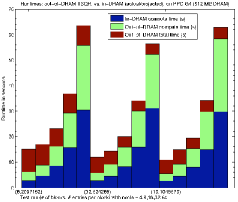
(a) Measured data

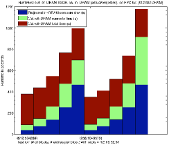
(b) Extrapolated runtime

Fig. 2: Runtimes (in seconds) of out-of-DRAM TSQR compared against (a) measured data and (b) extrapolated runtime of standard QR (LAPACK’s DGEQRF) on a single-processor laptop. For the measured data, we limit memory usage to 256 MB, which is half of the laptop’s total system memory, so that we can collect performance data for DGEQRF. For extrapolated data, we use the measured data to construct a power-law performance extrapolation. The graphs show different choices of block dimensions and number of blocks $P$. The top of the blue bar is (a) the benchmarked total runtime for DGEQRF and (b) the extrapolated total runtime for DGEQRF, the top of the green bar is the benchmarked compute time for TSQR, and the top of the brown bar is the benchmarked total time for TSQR. Thus the height of the brown bar alone is the I/O time. Note that LAPACK starts and ends in DRAM (if it could fit in DRAM), and TSQR starts and ends on disk.

Figure 2(a) shows the measured in-DRAM results on the laptop platform, and Figure 2(b) shows the (measured TSQR, extrapolated LAPACK) out-of-DRAM results on the same platform. In these figures, the amount of memory, and so the total number of matrix entries is constant for all the experiments: $m\cdot n=2^{2}4$. This means the total volume of communication is the same for all experiments. The number of blocks $P$ used, and so the number of matrix entries per block $mn/P$, is the same for each group of five bars, and is shown in a label under the horizontal axis. Within each group of 5 bars, we varied the number of matrix columns to be 4, 8, 16, 32, and 64. Note that we have not tried to overlap I/O and computation in this implementation. The trends in Figure 2(a) suggest that the extrapolation is reasonable: TSQR takes about twice as much time for computation as does standard LAPACK QR, and the fraction of time spent in I/O is reasonable and decreases with problem size.

TSQR assumes that the matrix starts and ends on disk, whereas LAPACK starts and ends in DRAM. Thus, to compare the two, one could also estimate LAPACK performance with infinite DRAM but where the data starts and ends on disk. The height of the reddish-brown bars in Figures 2(a) and 2(b) is the I/O time for TSQR, which can be used to estimate the LAPACK I/O time. This is reasonable since the volume of communication in the two cases is the same, and the fact that the reddish-brown bars are of similar height for different values of $P$, shows that the communication is bandwidth dominated. Add this to the blue bar (the LAPACK compute time) to estimate the runtime when the LAPACK QR routine must load the matrix from disk and store the results back to disk.

The main purpose of our out-of-DRAM code is not to outperform existing in-DRAM algorithms, but to be able to solve classes of problems which the existing algorithms cannot solve. The above graphs show that the penalty of an explicitly swapping approach is about 2x, which is small enough to warrant its practical use. This holds even for problems with a relatively low computational intensity, such as when the input matrix has very few columns. Furthermore, picking the number of columns sufficiently large may allow complete overlap of file I/O by computation.

7.2 Tests of parallel TSQR on a binary tree

# procs	CholeskyQR	TSQR	CGS	MGS	TSQR	ScaLAPACK
		(DGEQR3)			(DGEQRF)	(PDGEQRF)
1	1.02	4.14	3.73	7.17	9.68	12.63
2	0.99	4.00	6.41	12.56	15.71	19.88
4	0.92	3.35	6.62	12.78	16.07	19.59
8	0.92	2.86	6.87	12.89	11.41	17.85
16	1.00	2.56	7.48	13.02	9.75	17.29
32	1.32	2.82	8.37	13.84	8.15	16.95
64	1.88	5.96	15.46	13.84	9.46	17.74

Table 4: Runtime in seconds of various parallel QR factorizations on the Beowulf machine. The total number of rows $m=100000$ and the ratio $\lceil n/\sqrt{P}\rceil=50$ (with $P$ being the number of processors) were kept constant as $P$ varied from 1 to 64. This illustrates weak scaling with respect to the square of the number of columns $n$ in the matrix, which is of interest because the number of floating-point operations in sequential QR is $\mathcal{O}(mn^{2})$. If an algorithm scales perfectly, then all the runtimes in that algorithm’s column should be constant. Both the $Q$ and $R$ factors were computed explicitly; in particular, for those codes which form an implicit representation of $Q$, the conversion to an explicit representation was included in the runtime measurement.

# procs	CholeskyQR	TSQR	CGS	MGS	TSQR	ScaLAPACK
		(DGEQR3)			(DGEQRF)	(PDGEQRF)
1	0.45	3.43	3.61	7.13	7.07	7.26
2	0.47	4.02	7.11	14.04	11.59	13.95
4	0.47	4.29	6.09	12.09	13.94	13.74
8	0.50	4.30	7.53	15.06	14.21	14.05
16	0.54	4.33	7.79	15.04	14.66	14.94
32	0.52	4.42	7.85	15.38	14.95	15.01
64	0.65	4.45	7.96	15.46	14.66	15.33

Table 5: Runtime in seconds of various parallel QR factorizations on the Beowulf machine, illustrating weak scaling with respect to the total number of rows $m$ in the matrix. The ratio $\lceil m/P\rceil=100000$ and the total number of columns $n=50$ were kept constant as the number of processors $P$ varied from 1 to 64. If an algorithm scales perfectly, then all the runtimes in that algorithm’s column should be constant. For those algorithms which compute an implicit representation of the $Q$ factor, that representation was left implicit.

# procs	CholeskyQR	TSQR	CGS	MGS	TSQR	ScaLAPACK
		(DGEQR3)			(DGEQRF)	(PDGEQRF)
32	0.140	0.453	0.836	0.694	1.132	1.817
64	0.075	0.235	0.411	0.341	0.570	0.908
128	0.038	0.118	0.180	0.144	0.247	0.399
256	0.020	0.064	0.086	0.069	0.121	0.212

Table 6: Runtime in seconds of various parallel QR factorizations on the Frost machine on a $10^{6}\times 50$ matrix. This metric illustrates strong scaling (constant problem size, but number of processors increases).

We also present results for a parallel MPI implementation of TSQR on a binary tree. Rather than LAPACK’s DGEQRF, the code uses a custom local QR factorization, DGEQR3, based on the recursive approach of Elmroth and Gustavson [12]. Tests show that DGEQR3 consistently outperforms LAPACK’s DGEQRF by a large margin for matrix dimensions of interest.

We ran parallel TSQR on the following distributed-memory machines:

• Pentium III cluster (“Beowulf”), operated by the University of Colorado Denver. It has 35 dual-socket 900 MHz Pentium III nodes with Dolphin interconnect. Peak floating-point rate is 900 Mflop/s per processor, network latency is less than 2.7 $\mu$s, benchmarked, and network bandwidth is 350 MB/s, benchmarked upper bound.

• IBM BlueGene/L (“Frost”), operated by the National Center for Atmospheric Research. We use one BlueGene/L rack with 1024 700 MHz compute CPUs. Peak floating-point rate is 2.8 Gflop/s per processor, network latency is 1.5 $\mu$s, hardware, and network one-way bandwidth is 350 MB/s, hardware.

The experiments compare many different implementations of a parallel QR factorization. TSQR was tested both with the recursive local QR factorization DGEQR3, and the standard LAPACK routine DGEQRF. Both CGS and MGS (by row) were timed.

Tables 4 and 5 show the results of two different performance experiments on the Pentium III cluster. In the first of these, the total number of rows $m=100,000$ and the ratio $\lceil n/\sqrt{P}\rceil=50$ (with $P$ being the number of processors) were kept constant as $P$ varied from $1$ to $64$. This was meant to illustrate weak scaling with respect to $n^{2}$ (the square of the number of columns in the matrix), which is of interest because the number of floating-point operations in sequential QR is $\mathcal{O}(mn^{2})$. If an algorithm scales perfectly, then all the runtimes shown in that algorithm’s column should be constant. Both the tall and skinny $Q$ and the square $R$ factors were computed explicitly; in particular, for those codes which form an implicit representation of $Q$, the conversion to an explicit representation was included in the runtime measurement. The results show that TSQR scales better than CGS or MGS (by row), and significantly outperforms ScaLAPACK’s QR. Also, using the recursive local QR in TSQR, rather than LAPACK’s QR, more than doubles performance. CholeskyQR gets the best performance of all the algorithms, but at the expense of significant loss of orthogonality when the initial matrix $A$ is ill-conditioned. Note that, in this case ($Q$ and $R$ requested), CholeskyQR, CGS, and MGS perform half the flops of the Householder based algorithms, TSQR-DGEQR3, TSQR-DGEQRF, and PDGEQRF ($2mn^{2}$ versus $4mn^{2}$).

Table 5 shows the results of the second set of experiments on the Pentium III cluster. In these experiments, we also illustrate weak scaling with respect to the total number of rows $m$ in the matrix. For this, the ratio $\lceil m/P\rceil=100,000$ and the total number of columns $n=50$ were kept constant as the number of processors $P$ varied from 1 to 64. Unlike in the previous set of experiments, for those algorithms which compute an implicit representation of the $Q$ factor, that representation was left implicit. The results show that TSQR scales well. In particular, when using TSQR with the recursive local QR factorization, there is almost no performance penalty for moving from one processor to two, unlike with CGS, MGS, and ScaLAPACK’s QR. Again, the recursive local QR significantly improves TSQR performance; here it is the main factor in making TSQR perform better than ScaLAPACK’s QR. Note that, in this case (only $R$ requested), CholeskyQR, performs half the flops of all the others algorithm CGS, MGS, TSQR-DGEQR3, TSQR-DGEQRF, and PDGEQRF ($mn^{2}$ versus $2mn^{2}$).

Table 6 shows the results of the third set of experiments, which was performed on the BlueGene/L cluster “Frost.” These data show performance per processor (Mflop / s / (number of processors)) on a matrix of constant dimensions $10^{6}\times 50$, as the number of processors was increased. This illustrates strong scaling. If an algorithm scales perfectly, then all the numbers in that algorithm’s column should decrease proportionally to $P$, i.e. halve from row to row. For ScaLAPACK’s QR factorization, we used PDGEQRF. We observe that using the recursive local QR factorization with TSQR makes it clearly outperfom ScaLAPACK. Note that, in this case ($Q$ and $R$ requested), CholeskyQR, CGS, and MGS perform half the flops of the Householder based algorithms, TSQR-DGEQR3, TSQR-DGEQRF, and PDGEQRF ($2mn^{2}$ versus $4mn^{2}$).

Both the Pentium III and BlueGene/L platforms have relatively slow processors with a relatively low-latency interconnect. TSQR was optimized for the opposite case of fast processors and expensive communication. Nevertheless, TSQR outperforms ScaLAPACK’s QR by over $6.7\times$ on 16 processors (and $3.5\times$ on 64 processors) on the Pentium III cluster, and $4.0\times$ on 32 processors (and $3.3\times$ on 256 processors) on the BlueGene/L machine.

7.3 Performance estimation of parallel CAQR

We use the performance model developed in Section 6 to estimate the performance of parallel CAQR on a model of a petascale machine. We expect CAQR to outperform ScaLAPACK, in part because it uses a faster algorithm for performing most of the computation of each panel factorization (DGEQR3 vs. DGEQRF), and in part because it reduces the latency cost. Our performance model uses the same time per floating-point operation for both CAQR and PDGEQRF. Hence our model evaluates the improvement due only to reducing the latency cost.

Our projection of a future petascale machine (“Peta”) has 8192 processors. Each “processor” of Peta may itself be a parallel multicore node, but we consider it as a single fast sequential processor for the sake of our model. Here are the parameters we use:

• Peta. Peak floating-point rate is 500 Gflop/s per processor, network latency is 10 $\mu$s, and network bandwidth is 4 GB/s.

We evaluate the performance using matrices of size $n\times n$, distributed over a $P_{r}\times P_{c}$ grid of $P$ processors using a 2D block cyclic distribution, with square blocks of size $b\times b$. We estimate the best performance of CAQR and PDGEQRF for a given problem size $n$ and a given number of processors $P$, by finding the optimal values for the block size $b$ and the shape of the grid $P_{r}\times P_{c}$ in the allowed ranges. The matrix size $n$ is varied in the range $10^{3}$, $10^{3.5}$, $10^{4}$, $\dots$, $10^{7.5}$. The block size $b$ is varied in the range $1$, $5$, $10$, $\dots$, $50$, $60$, $\dots$, $\min(200,m/P_{r},n/P_{c})$. The number of processors is varied from $1$ to the largest power of $2$ smaller than $p_{max}$, in which $p_{max}$ is the maximum number of processors available in the system. The values for $P_{r}$ and $P_{c}$ are also chosen to be powers of two.

When we evaluate the model, we set the floating-point performance value in the model so that the modeled floating-point rate is 80% of the machine’s peak rate, so as to capture realistic performance on the local QR factorizations. The inverse network bandwidth $\beta$ has units of seconds per word. The white regions in the plots signify that the problem needed more memory than available on the machine.

Figure 3 shows our performance estimates of CAQR and PDGEQRF on the Petascale machine, in which we display

• Figure 3(a) – the best speedup obtained by CAQR, with respect to the runtime using the fewest number of processors with enough memory to hold the matrix (which may be more than one processor),

• Figure 3(b) – the best speedup obtained by PDGEQRF, computed similarly, and

• Figure 3(c) – the ratio of PDGEQRF runtime to CAQR runtime.

As can be seen in Figure 3(a), CAQR is expected to show good scalability for large matrices. For example, for $n=10^{5.5}$, a speedup of $1431$, measured with respect to the time on $2$ processors, is obtained on $8192$ processors. For $n=10^{6}$ a speedup of $167$, measured with respect to the time on $32$ processors, is obtained on $8192$ processors.

In the technical report [9], we also estimate the fractions of time in computation, latency, and bandwidth for PDGEQRF and CAQR. These estimations show that for the largest problems that can fit in memory, in the top left part of the plots in Figure 3, the computation dominates the total time, while in the right bottom part the latency dominates the total time. For the test cases situated between these two parts, the bandwidth dominates the time.

CAQR leads to more significant improvements when the latency represents an important fraction of the total time, the right bottom part of Figure 3(c). The best improvement is a factor of $22.9$, obtained for $n=10^{4}$ and $P=8192$. The speedup of the best CAQR compared to the best PDGEQRF for $n=10^{4}$ when using at most $P=8192$ processors is larger than $8$, which is still an important improvement. The best performance of CAQR is obtained for $P=4096$ processors and the best performance of PDGEQRF is obtained for $P=16$ processors.

Useful improvements are also obtained for larger matrices. For $n=10^{6}$, CAQR outperforms PDGEQRF by a factor of $1.4$. When the computation dominates the parallel time, Figure 3(c) predicts that there is no benefit from using CAQR. However, CAQR is never slower. For any fixed $n$, we can take the number of processors $P$ for which PDGEQRF would perform the best, and measure the speedup of CAQR over PDGEQRF using that number of processors. We do this in Table 7, which predicts that CAQR always is at least as fast as PDGEQRF, and often significantly faster (up to $7.4\times$ faster in some cases).

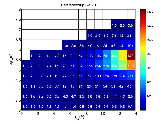
(a) Speedup CAQR

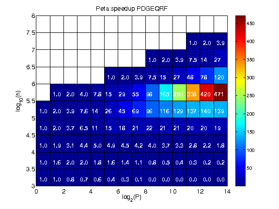
(b) Speedup PDGEQRF

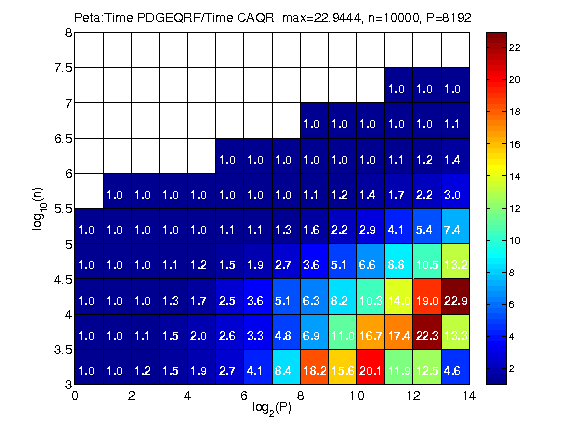
(c) Comparison

Fig. 3: Performance prediction comparing CAQR and PDGEQRF on Peta.

$\log_{10}n$	Best $\log_{2}P$ for PDGEQRF	CAQR speedup
3.0	1	1
3.5	2–3	1.1–1.5
4.0	4–5	1.7–2.5
4.5	7–10	2.7–6.6
5.0	11–13	4.1–7.4
5.5	13	3.0
6.0	13	1.4

Table 7: Estimated runtime of PDGEQRF divided by estimated runtime of parallel CAQR on a square $n\times n$ matrix, on the Peta platform, for those values of $P$ (number of processors) for which PDGEQRF performs the best for that problem size.

8 Conclusions and Future Work

We have presented sequential and parallel algorithms that minimize the communication performed during the QR factorization of tall and skinny matrices and general rectangular matrices. In the accompanying paper [8] we have shown that the new algorithms are optimal in the amount of communication they perform, thus they are superior in theory over existing algorithms. In this paper we have presented implementations demonstrating in practice significant speedups over LAPACK and ScaLAPACK. In particular, we have studied the performance of parallel TSQR on a binary tree and sequential TSQR on a flat tree.

Implementations of parallel CAQR are currently underway. Optimization of the TSQR reduction tree for more general, practical architectures (such as multicore, multisocket, or GPUs) is future work, as well as optimization of the rest of CAQR to the most general architectures, with proofs of optimality.

It is natural to ask to how much of dense linear algebra one can extend the results of this paper, that is finding algorithms that attain communication lower bounds. In the case of parallel LU with pivoting, refer to the paper by Grigori, Demmel, and Xiang [16], and in the case of sequential LU, refer to the paper by Toledo [33]. More broadly, we hope to extend the results of this paper to other linear algebra operations, including two-sided factorizations (such as reduction to symmetric tridiagonal, bidiagonal, or (generalized) upper Hessenberg forms). Once a matrix is symmetric tridiagonal (or bidiagonal) and so takes little memory, fast algorithms for the eigenproblem (or SVD) are available. Most challenging is likely to be finding eigenvalues of a matrix in upper Hessenberg form (or of a matrix pencil).

References

- [1] M. Baboulin, L. Giraud, S. Gratton, and J. Langou, Parallel tools for solving incremental dense least squares problems. Application to space geodesy, Tech. Report UT-CS-06-582, University of Tennessee, Sept. 2006. LAWN #179.
- [2] J. Baglama, D. Calvetti, and L. Reichel, Algorithm 827: irbleigs: A MATLAB program for computing a few eigenpairs of a large sparse Hermitian matrix, ACM Trans. Math. Softw., 29 (2003), pp. 337–348.
- [3] Z. Bai and D. Day, Block Arnoldi method, in Templates for the Solution of Algebraic Eigenvalue Problems: A Practical Guide, Z. Bai, J. W. Demmel, J. J. Dongarra, A. Ruhe, and H. van der Vorst, eds., Society for Industrial and Applied Mathematics, Philadelphia, PA, USA, 2000, pp. 196–204.
- [4] C. G. Baker, U. L. Hetmaniuk, R. B. Lehoucq, and H. K. Thornquist, Anasazi webpage. http://trilinos.sandia.gov/packages/anasazi/.
- [5] A. Buttari, J. Langou, J. Kurzak, and J. J. Dongarra, A class of parallel tiled linear algebra algorithms for multicore architectures, Tech. Report UT-CS-07-600, University of Tennessee, Sept. 2007. LAWN #191.
- [6] R. D. Da Cunha, D. Becker, and J. C. Patterson, New parallel (rank-revealing) QR factorization algorithms, in Euro-Par 2002. Parallel Processing: Eighth International Euro-Par Conference, Paderborn, Germany, August 27–30, 2002, 2002.
- [7] E. D’Azevedo and J. Dongarra, The design and implementation of the parallel out-of-core ScaLAPACK LU, QR, and Cholesky factorization routines, Concurrency Practice and Experience, 12 (2000), pp. 1481–1483.
- [8] J. W. Demmel, L. Grigori, M. Hoemmen, and J. Langou, Communication-avoiding parallel and sequential QR and LU factorizations. Submitted to SIAM Journal of Scientific Computing, 2008.
- [9] , Communication-avoiding parallel and sequential QR and LU factorizations: theory and practice, Tech. Report UCB/EECS-2008-89, University of California Berkeley, EECS Department, 2008. LAWN #204.
- [10] J. W. Demmel and M. Hoemmen, Communication-avoiding Krylov subspace methods, tech. report, University of California Berkeley, Department of Electrical Engineering and Computer Science, in preparation.
- [11] E. Elmroth and F. Gustavson, New serial and parallel recursive QR factorization algorithms for SMP systems, in Applied Parallel Computing. Large Scale Scientific and Industrial Problems., B. Kågström et al., ed., vol. 1541 of Lecture Notes in Computer Science, Springer, 1998, pp. 120–128.
- [12] , Applying recursion to serial and parallel QR factorization leads to better performance, IBM Journal of Research and Development, 44 (2000), pp. 605–624.
- [13] R. W. Freund and M. Malhotra, A block QMR algorithm for non-Hermitian linear systems with multiple right-hand sides, Linear Algebra and its Applications, 254 (1997), pp. 119–157. Proceedings of the Fifth Conference of the International Linear Algebra Society (Atlanta, GA, 1995).
- [14] G. H. Golub and C. F. Van Loan, Matrix Computations, The Johns Hopkins University Press, Baltimore, MD, USA, third ed., 1996.
- [15] G. H. Golub, R. J. Plemmons, and A. Sameh, Parallel block schemes for large-scale least-squares computations, in High-Speed Computing: Scientific Applications and Algorithm Design, Robert B. Wilhelmson, ed., University of Illinois Press, Urbana and Chicago, IL, USA, 1988, pp. 171–179.
- [16] L. Grigori, J. W. Demmel, and H. Xiang, Communication avoiding Gaussian elimination, Proceedings of the ACM/IEEE SC08 Conference, (2008).
- [17] W. Gropp, E. Lusk, and A. Skjellum, Using MPI: Portable Parallel Programming with the Message-Passing Interface, MIT Press, 1999.
- [18] B. C. Gunter and R. A. van de Geijn, Parallel out-of-core computation and updating of the QR factorization, ACM Transactions on Mathematical Software, 31 (2005), pp. 60–78.
- [19] U. Hetmaniuk and R. Lehoucq, Basis selection in LOBPCG, Journal of Computational Physics, 218 (2006), pp. 324–332.
- [20] A. V. Knyazev, BLOPEX webpage. http://www-math.cudenver.edu/~aknyazev/software/BLOPEX/.
- [21] A. V. Knyazev, M. Argentati, I. Lashuk, and E. E. Ovtchinnikov, Block locally optimal preconditioned eigenvalue xolvers (BLOPEX) in HYPRE and PETSc, Tech. Report UCDHSC-CCM-251P, University of California Davis, 2007.
- [22] J. Kurzak and J. J. Dongarra, QR factorization for the CELL processor, Tech. Report UT-CS-08-616, University of Tennessee, May 2008. LAWN #201.
- [23] R. Lehoucq and K. Maschhoff, Block Arnoldi method, in Templates for the Solution of Algebraic Eigenvalue Problems: A Practical Guide, Z. Bai, J. W. Demmel, J. J. Dongarra, A. Ruhe, and H. van der Vorst, eds., Society for Industrial and Applied Mathematics, Philadelphia, PA, USA, 2000, pp. 185–187.
- [24] O. Marques, BLZPACK webpage. http://crd.lbl.gov/~osni/.
- [25] R. Nishtala, G. Almási, and C. Caşcaval, Performance without pain = productivity: Data layout and collective communication in UPC, in Proceedings of the ACM SIGPLAN 2008 Symposium on Principles and Practice of Parallel Programming, 2008.
- [26] D. P. O’Leary, The block conjugate gradient algorithm and related methods, Linear Algebra and its Applications, 29 (1980), pp. 293–322.
- [27] A. Pothen and P. Raghavan, Distributed orthogonal factorization: Givens and Householder algorithms, SIAM J. Sci. Stat. Comput., 10 (1989), pp. 1113–1134.
- [28] G. Quintana-Ortí, E. S. Quintana-Ortí, E. Chan, F. G. Van Zee, and R. A. van de Geijn, Scheduling of QR factorization algorithms on SMP and multi-core architectures, in Proceedings of the 16th Euromicro International Conference on Parallel, Distributed and Network-Based Processing, Toulouse, France, Feb. 2008. FLAME Working Note #24.
- [29] E. Rabani and S. Toledo, Out-of-core SVD and QR decompositions, in Proceedings of the 10th SIAM Conference on Parallel Processing for Scientific Computing, Norfolk, Virginia, SIAM, Mar. 2001.
- [30] R. Schreiber and C. Van Loan, A storage efficient representation for products of Householder transformations, SIAM J. Sci. Stat. Comput., 10 (1989), pp. 53–57.
- [31] A. Stathopoulos, PRIMME webpage. http://www.cs.wm.edu/~andreas/software/.
- [32] A. Stathopoulos and K. Wu, A block orthogonalization procedure with constant synchronization requirements, SIAM Journal on Scientific Computing, 23 (2002), pp. 2165–2182.
- [33] S. Toledo, Locality of reference in LU decomposition with partial pivoting, SIAM J. Matrix Anal. Appl., 18 (1997), pp. 1065–1081.
- [34] B. Vital, Étude de quelques méthodes de résolution de problèmes linéaires de grande taille sur multiprocesseur, Ph.D. dissertation, Université de Rennes I, Rennes, Nov. 1990.
- [35] K. Wu and H. D. Simon, TRLAN webpage. http://crd.lbl.gov/~kewu/ps/trlan_.html.