Estimation of a probability with optimum guaranteed confidence in inverse binomial sampling

Abstract

Sequential estimation of a probability $p$ by means of inverse binomial sampling is considered. For $\mu_{1},\mu_{2}>1$ given, the accuracy of an estimator $\hat{p}$ is measured by the confidence level $P[p/\mu_{2}\leq\hat{p}\leq p\mu_{1}]$. The confidence levels $c_{0}$ that can be guaranteed for $p$ unknown, that is, such that $P[p/\mu_{2}\leq\hat{p}\leq p\mu_{1}]\geq c_{0}$ for all $p\in(0,1)$, are investigated. It is shown that within the general class of randomized or non-randomized estimators based on inverse binomial sampling, there is a maximum $c_{0}$ that can be guaranteed for arbitrary $p$. A non-randomized estimator is given that achieves this maximum guaranteed confidence under mild conditions on $\mu_{1}$, $\mu_{2}$.

and

1 Introduction

In a sequence of Bernoulli trials with probability of success $p$ at each trial, consider the estimation of $p$ by inverse binomial sampling. This sampling scheme, first discussed by Haldane (1945), consists in observing the sequence until a given number $r$ of successes is obtained. The resulting number of trials $N$ is a sufficient statistic for $p$ (Lehmann and Casella (1998), page 101). The uniformly minimum variance unbiased estimator of $p$ is (Mikulski and Smith (1976))

$$\hat{p}=\frac{r-1}{N-1}$$ (1)

and for $r\geq 3$, it has a normalized mean square error $\mathrm{E}[(\hat{p}-p)^{2}]/p^{2}$ (or $\operatorname{Var}[\hat{p}]/p^{2}$) lower than $1/(r-2)$, irrespective of $p$ (Mikulski and Smith (1976); Sathe (1977); Prasad and Sahai (1982)).

This paper analyzes inverse binomial sampling from a different point of view, related to interval estimation. Given $\mu_{1},\mu_{2}>1$, the accuracy of an estimator $\hat{p}$ is measured by the probability $c$ that $\hat{p}$ lies in the interval $[p/\mu_{2},p\mu_{1}]$. The motivation to use a relative interval $[p/\mu_{2},p\mu_{1}]$, instead of an interval $[x_{1},x_{2}]$ with $x_{1},x_{2}$ fixed, is the fact that $P[p/\mu_{2}\leq\hat{p}\leq p\mu_{1}]$, unlike $P[x_{1}\leq\hat{p}\leq x_{2}]$, has a definite meaning independent of $p$. Moreover, using a relative interval allows another interpretation of $c$: since $p/\mu_{2}\leq\hat{p}\leq p\mu_{1}$ if and only if $\hat{p}/\mu_{1}\leq p\leq\hat{p}\mu_{2}$, $c$ gives the probability that the true value $p$ is covered by the random interval $[\hat{p}/\mu_{1},\hat{p}\mu_{2}]$. In the sequel, $c$ will be referred to as the confidence (or confidence level) associated with $\mu_{1}$, $\mu_{2}$.

Recently, Mendo and Hernando (2006; 2008a) have shown that the estimator

$$\hat{p}=\frac{r-1}{N}$$ (2)

has the following properties for $r\geq 3$. The confidence level $c$ associated with $\mu_{1}$, $\mu_{2}$ has an asymptotic value $\bar{c}$ as $p\rightarrow 0$, namely $\bar{c}=\gamma(r,(r-1)\mu_{2})-\gamma(r,(r-1)/\mu_{1}),$ where

$$\gamma(r,t)=\frac{1}{\Gamma(r)}\int_{0}^{t}s^{r-1}\exp(-s)\,\mathrm{d}s$$

is the regularized incomplete gamma function. Furthermore, the confidence for any $p\in(0,1)$ exceeds this asymptotic value provided that $\mu_{1}$ and $\mu_{2}$ satisfy certain lower bounds. Similar results have been established (Mendo and Hernando, 2008b) for the uniformly minimum variance unbiased estimator (1). Using a more general setting in which the Bernoulli random variables are replaced by arbitrary bounded random variables, Chen (2007) has obtained comparable (although somewhat less tight) results for (1), as well as for the maximum likelihood estimator

$$\hat{p}=\frac{r}{N}.$$ (3)

From the aforementioned results, the question naturally arises as to whether the attained confidence could be improved using estimators other than (1)–(3). This motivates the study of arbitrary estimators based on inverse binomial sampling. In this regard, it is noted that $1-c$ can be expressed as the risk $\mathrm{E}[L(\hat{p})]$ corresponding to the loss function $L$ defined as

$$L(x)=\cases{0,&\quad if $x\in[p/\mu_{2},p\mu_{1}]$,\cr 1,&\quad otherwise.}$$ (4)

Since $N$ is a sufficient statistic, for any estimator defined in terms of the observed Bernoulli random variables, there exists an estimator that depends on the observations through $N$ only and that has the same risk; this equivalent estimator is possibly a randomized one (Lehmann and Casella (1998), page 33). (The fact that $L$ is non-convex prevents application of a corollary of the Rao–Blackwell theorem (Lehmann and Casella (1998), page 48) to discard randomized estimators.) Thus, attention can be restricted to estimators that depend on the observed variables only through $N$; however, both randomized and non-randomized estimators have to be considered.

The purpose of the present paper is to investigate the limits on the confidence levels $c_{0}$ that can be guaranteed (in the sense that the actual confidence equals or exceeds $c_{0}$, irrespective of $p$) in inverse binomial sampling. More specifically, the objectives are:

• to determine the supremum of $\inf_{p\in(0,1)}c$ over all (randomized or non-randomized) estimators based on inverse binomial sampling;

• to find an estimator, if it exists, that can achieve this supremum.

Consequently, the main focus of this paper is on non-asymptotic results, valid for $p\in(0,1)$. Nonetheless, asymptotic results for $p\rightarrow 0$ will also be derived since, apart from their own theoretical importance, they provide an upper bound on (and an indication of) what can be achieved for arbitrary $p$.

Section 2 shows that $\liminf_{p\rightarrow 0}c$ has a maximum over all estimators based on inverse binomial sampling and computes this maximum. This sets an upper bound on the confidence that can be guaranteed by an arbitrary estimator. Section 3 establishes that this upper bound is also a maximum, that is, estimators exist that can achieve this guaranteed confidence. Specifically, estimators are given that guarantee the maximum confidence for sufficiently small $p$ and that guarantee the maximum confidence for any $p$, under certain conditions on the relative interval being considered. Section 4 discusses the results, comparing them with those from other works. Section 5 contains proofs of all results in the paper.

2 Asymptotic analysis

It is assumed in the sequel that $r\geq 3$. Let $t^{(j)}$ denote $t(t-1)\cdots(t-j+1)$. The probability function of $N$, $f(n)=P[N=n]$, is

$$f(n)=\frac{(n-1)^{(r-1)}}{(r-1)!}p^{r}(1-p)^{n-r}\qquad\mbox{for }n\geq r.$$ (5)

As justified in Section 1, it is sufficient to consider (possibly randomized) estimators defined in terms of the sufficient statistic $N$. Let $\mathcal{F}$ denote the set of all functions from $\{r,r+1,r+2,\ldots\}$ to $\mathbb{R}$. A non-randomized estimator $\hat{p}$ can be described as $\hat{p}=g(N)$, with $g\in\mathcal{F}$. Thus, a non-randomized estimator is entirely specified by its function $g$. A randomized estimator is a random variable $\hat{p}$ whose distribution depends, in general, on the value taken by $N$. Let $\Pi_{n}$ denote the distribution function of $\hat{p}$ conditioned on $N=n$. The randomized estimator is completely specified by the functions $\Pi_{n}$, $n\geq r$. Thus, denoting by $\mathcal{F}_{\mathcal{R}}$ the class of all functions from $\{r,r+1,r+2,\ldots\}$ to the set of real functions of a real variable, a randomized estimator is defined by a function $G\in\mathcal{F}_{\mathcal{R}}$ that assigns $\Pi_{n}$ to each $n$.

Non-randomized estimators form a subset of the class of randomized estimators. Thus, any statement that applies to randomized estimators will also be valid, in particular, for non-randomized estimators. The reason that the specialized class of non-randomized estimators has been explicitly defined is that, on one hand, their simplicity makes them more attractive for applications and, on the other hand, it will be seen that, under certain conditions, no loss of optimality in guaranteed confidence is incurred by restricting to non-randomized estimators. Throughout the paper, when referring to an arbitrary estimator without specifying its type, the general class of randomized estimators (including the non-randomized ones) will be meant.

Given any estimator $G\in\mathcal{F}_{\mathcal{R}}$, the confidence associated with $\mu_{1}$, $\mu_{2}$ will be expressed in the sequel as a function $c(p)$ (that is, the dependence on $p$ will be explicitly indicated). Given $r$, $\mu_{1}$ and $\mu_{2}$, the latter function is determined by $G$. An estimator is said to guarantee a confidence level $c_{0}$ in the interval $(p_{1},p_{2})$ if $c(p)\geq c_{0}$ for all $p\in(p_{1},p_{2})$. If the interval is $(0,1)$, then the estimator is said to globally guarantee this confidence level. An estimator asymptotically guarantees a certain $c_{0}$ if there exists $\varepsilon>0$ such that the estimator guarantees $c_{0}$ in the interval $(0,\varepsilon)$.

The problem being addressed can be rephrased as that of optimizing the globally guaranteed confidence within the general class of estimators based on inverse binomial sampling, or finding a minimax estimator with respect to the risk defined by the loss function (4). The following proposition, and its ensuing particularization, provides the motivation for studying $\liminf_{p\rightarrow 0}c(p)$ as part of this optimization problem.

Proposition 1

If a given estimator, with confidence function $c(p)$, guarantees a confidence level $c_{0}$ in an interval $(p_{1},p_{2})$, then, necessarily, $\liminf_{p\rightarrow p_{0}}c(p)\geq c_{0}$ for any $p_{0}\in[p_{1},p_{2}]$.

Particularizing Proposition 1 to $p_{1}=p_{0}=0$, it is seen that $\liminf_{p\rightarrow 0}c(p)$ represents an upper bound on the confidence levels that can be globally or asymptotically guaranteed.

An important subclass of non-randomized estimators is formed by those defined by functions $g\in\mathcal{F}$ for which $c(p)$ has an asymptotic value, that is, for which $\lim_{p\rightarrow 0}P[p/\mu_{2}\leq g(N)\leq p\mu_{1}]$ exists. The set of all such functions will be denoted $\mathcal{F}_{\mathrm{p}}$. As will be seen, another important subclass is that corresponding to the set of functions $g\in\mathcal{F}$ for which $\lim_{n\rightarrow\infty}ng(n)$ exists, is finite and non-zero. This set will be denoted $\mathcal{F}_{\mathrm{n}}$. The following result establishes that $\mathcal{F}_{\mathrm{n}}\subset\mathcal{F}_{\mathrm{p}}$.

Proposition 2

For a non-randomized estimator defined by $g\in\mathcal{F}_{\mathrm{n}}$, $\lim_{p\rightarrow 0}c(p)$ exists and equals $\bar{c}$, given by

$$\bar{c}=\gamma(r,\Omega\mu_{2})-\gamma(r,\Omega/\mu_{1}),\qquad\Omega=\lim_{n\rightarrow\infty}ng(n).$$ (6)

The converse of Proposition 2 is not true; that is, $\mathcal{F}_{\mathrm{n}}\neq\mathcal{F}_{\mathrm{p}}$. A simple counterexample is given by

$$g(n)=\cases{{\omega^{\prime}}/{n},&\quad if there exists $k\in\mathbb{N}$ such that $n=2^{k}$,\cr{\omega}/{n},&\quad otherwise,}$$

with $\omega^{\prime}\neq\omega$. It is easily seen that this function is in $\mathcal{F}_{\mathrm{p}}$, with $\lim_{p\rightarrow 0}c(p)=\gamma(r,\omega\mu_{2})-\gamma(r,\omega/\mu_{1})$; however, $\lim_{n\rightarrow\infty}ng(n)$ does not exist.

Given $r$, $\mu_{1}$ and $\mu_{2}$, the maximum of $\bar{c}$ over all $g\in\mathcal{F}_{\mathrm{n}}$ is attained when $\lim_{n\rightarrow\infty}ng(n)$ equals $\Omega^{*}$, given by

$$\Omega^{*}=r\frac{\log\mu_{2}-\log(1/\mu_{1})}{\mu_{2}-1/\mu_{1}},$$ (7)

as is readily seen by differentiating $\bar{c}$ in (6). Let $c^{*}$ denote the resulting maximum. Defining

$$M=\mu_{1}\mu_{2},$$ (8)

the terms $\Omega^{*}/\mu_{1}$ and $\Omega^{*}\mu_{2}$ can be expressed as

$$\Omega^{*}/\mu_{1}=\frac{r\log M}{M-1},\qquad\Omega^{*}\mu_{2}=\frac{rM\log M}{M-1}$$ (9)

and thus

$$c^{*}=\gamma\biggl{(}r,\frac{rM\log M}{M-1}\biggr{)}-\gamma\biggl{(}r,\frac{r\log M}{M-1}\biggr{)}.$$ (10)

The following theorem establishes that $c^{*}$ is not only the maximum of $\lim_{p\rightarrow 0}c(p)$ within the subclass of non-randomized estimators defined by $\mathcal{F}_{\mathrm{n}}$, but also the maximum of $\liminf_{p\rightarrow 0}c(p)$ within the general class of randomized estimators defined by $\mathcal{F}_{\mathcal{R}}$.

Theorem 1

The maximum of $\liminf_{p\rightarrow 0}c(p)$ over all estimators defined by functions $G\in\mathcal{F}_{\mathcal{R}}$ is $c^{*}$, given by (10).

As can be seen from (10), $c^{*}$ depends on $\mu_{1}$ and $\mu_{2}$ only through $M$. An explanation of this result is as follows. Given $\mu_{1}$, $\mu_{2}$, let $\hat{p}$ be an arbitrary estimator and consider $a>0$. If $\mu_{1}$ and $\mu_{2}$ are replaced by $\mu_{1}^{\prime}=a\mu_{1}$ and $\mu_{2}^{\prime}=\mu_{2}/a$, respectively, defining a modified estimator $\hat{p}^{\prime}=a\hat{p}$, it is clear that $p/\mu_{2}^{\prime}\leq\hat{p}^{\prime}\leq p\mu_{1}^{\prime}$ if and only if $p/\mu_{2}\leq\hat{p}\leq p\mu_{1}$. This shows that any value of $\liminf_{p\rightarrow 0}c(p)$ that can be achieved for $\mu_{1}$, $\mu_{2}$ can also be achieved for $a\mu_{1}$, $\mu_{2}/a$ (using a different estimator), and conversely. Thus, $c^{*}$ is the same for $\mu_{1}$, $\mu_{2}$ and for $a\mu_{1}$, $\mu_{2}/a$.

3 An optimum estimator for certain relative intervals

The asymptotic results in Section 2 impose a limit on the confidence levels that can be guaranteed, as established by the following corollary of Proposition 1 and Theorem 1.

Corollary 1

No estimator can guarantee a confidence level greater than $c^{*}$, given by (10), in an interval $(0,p_{2})$.

According to Corollary 1, $c^{*}$ is an upper bound on the confidence that can be guaranteed either asymptotically or globally. It remains to be seen if there exists some estimator that can actually guarantee the confidence level $c^{*}$. If it exists, that estimator will be optimum from the point of view of guaranteed confidence. A related question is if one such optimum estimator can be found within the restricted class of non-randomized estimators. As will be shown, the answer to both questions turns out to be affirmative for all values of $\mu_{1}$ and $\mu_{2}$ in the case of asymptotic guarantee and for certain values of $\mu_{1}$ and $\mu_{2}$ in the case of global guarantee.

Consider a non-randomized estimator $\hat{p}=g(N)$ of the form

$$g(n)=\frac{\Omega}{n+d},$$ (11)

where $\Omega$ and $d$ are parameters (with $\Omega=\lim_{n\rightarrow\infty}ng(n)$). This is a generalization of the estimators (1)–(3). Note that (11) has an asymptotic confidence $\bar{c}$ given by (6) and, for $\Omega=\Omega^{*}$, it achieves the maximum $\liminf_{p\rightarrow 0}c(p)$ that any estimator can have, according to Theorem 1.

Under a mild condition on $d$, the estimator given by (11) with $\Omega=\Omega^{*}$ can be shown to asymptotically guarantee the confidence $c^{*}$ for any $\mu_{1}$, $\mu_{2}>0$, as established by Theorem 2 below.

Theorem 2

The non-randomized estimator

$$\hat{p}=\frac{\Omega^{*}}{N+d}$$ (12)

asymptotically guarantees the optimum confidence $c^{*}$ given in (10) if

$$d>\frac{1}{2}\biggl{(}-r+\frac{M+1}{M-1}\biggr{)},$$ (13)

where $M$ is defined by (8).

An estimator of this form can also globally guarantee the confidence level $c^{*}$, provided that $\mu_{1}$, $\mu_{2}$ are not too small, as discussed in the following.

For $d\in\mathbb{Z}$, the estimator defined by (11) lends itself to an analysis similar to that carried out by Mendo and Hernando (2006; 2008a) for the particular case (2). This allows the derivation of sufficient conditions on $\mu_{1}$, $\mu_{2}$ which ensure that $c(p)\geq\bar{c}$ for all $p\in(0,1)$. The least restrictive conditions are obtained for $d=1$ and are given in the following proposition, which, particularized to $\Omega=\Omega^{*}$, will yield the desired result on globally guaranteeing the optimum confidence.

Proposition 3

The confidence of the non-randomized estimator

$$\hat{p}=\frac{\Omega}{N+1}$$ (14)

exceeds its asymptotic value $\bar{c}$, given by (6), for all $p\in(0,1)$ if

$$\mu_{1}\geq\frac{\Omega}{r-\sqrt{r}},\qquad\mu_{2}\geq\frac{r+\sqrt{r}+1}{\Omega}.$$ (15)

Particularizing to $\Omega=\Omega^{*}$, Proposition 3 establishes that there exists a non-randomized estimator that can globally guarantee the optimum confidence $c^{*}$ for certain values of $\mu_{1}$, $\mu_{2}$. It turns out that for $\Omega=\Omega^{*}$ and $r$ given, one of the two inequalities in (15) implies the other. Thus, for each $r$, only one of the inequalities needs to be considered in order to determine the allowed range for $\mu_{1}$, $\mu_{2}$. The result is stated in the following theorem.

Theorem 3

The non-randomized estimator

$$\hat{p}=\frac{\Omega^{*}}{N+1},$$ (16)

with $\Omega^{*}$ as in (7), globally guarantees the optimum confidence $c^{*}$ given by (10) if either of the following conditions is satisfied:

$$\frac{M-1}{\log M} \geq \frac{r+\sqrt{r}}{r-1}\qquad\mbox{for }r\in\{3,4\};$$ (17)

$$\frac{M\log M}{M-1} \geq \frac{r+\sqrt{r}+1}{r}\qquad\mbox{for }r\geq 5,$$ (18)

where $M$ is defined by (8). These conditions can be jointly expressed as $M\geq h(r)$, where $h$ is an increasing function.

Given $r$, consider the region of $(\mu_{1},\mu_{2})$ values that satisfy the appropriate condition (17) or (18), with $\mu_{1},\mu_{2}>1$. From Theorem 3, the boundary of this region is a continuous, decreasing, concave curve in $(1,\infty)\times(1,\infty)$, namely, the curve determined by the equation $\mu_{1}\mu_{2}=h(r)$. The region in question is the union of this curve and the portion of the plane lying above and to the right. Furthermore, the region for $r^{\prime}>r$ contains that for $r$.

According to the preceding results, the problem of optimum estimation of $p$, in the sense of globally guaranteeing the maximum possible confidence, is solved by the non-randomized estimator (16) for $\mu_{1}$, $\mu_{2}$ satisfying (17) or (18). Equivalently, this estimator is minimax with respect to the risk defined by the loss function given in (4) (maximin with respect to confidence).

The fact that $c^{*}$ depends on $\mu_{1}$, $\mu_{2}$ only through $M$ gives rise to another interpretation of the result in Theorem 3. For $r$ and $M$ given, consider the problem of finding, among all interval estimators of $p$ with a ratio $M$ between their end-points, that which maximizes the globally guaranteed confidence. The solution, if $M$ satisfies (17) or (18), is

$$\biggl{[}\frac{r\log M}{(M-1)(N+1)},\frac{rM\log M}{(M-1)(N+1)}\biggr{]}$$ (19)

and the resulting maximum is $c^{*}$, as expressed by (10). Equivalently, given $r$ and a prescribed confidence $c_{0}$, if a value for $M$ is computed such that (10) holds with $c^{*}=c_{0}$ and if it satisfies (17) or (18), then the interval estimator (19) minimizes the ratio between interval end-points subject to a globally guaranteed confidence level $c_{0}$. Observe that it is meaningful to prescribe, or minimize, the ratio of the interval end-points, rather than their difference, since a given value for the latter might be either unacceptably high or unnecessarily small, depending on the unknown $p$, whereas the ratio has a definite meaning, regardless of $p$.

According to Proposition 3, conditions (15) are sufficient; however, they may not be necessary. The same applies to (17) and (18). Determining the most general conditions which assure optimality of (16) is a difficult problem. Nevertheless, as will be illustrated, the sufficient conditions (17) or (18) cover most cases of interest.

4 Discussion

Figure 1(a) depicts the relationship between $c^{*}$, $M$ and $r$, for $M$ satisfying (17) or (18). The guaranteed confidence $c^{*}$ is represented, for convenience, as a function of $\sqrt{M}-1$, each dashed curve corresponding to a different $r$. The figure also represents, with solid line, the minimum $c^{*}$ that fulfills inequalities (17) or (18); this corresponds to the lowest $r$ for which the applicable inequality holds. Figure 1(b) shows this minimum $r$ as a function of $\sqrt{M}-1$, with $c^{*}$ as a parameter. From Corollary 1, this figure also has a more general interpretation as the minimum $r$ that is required in order to guarantee (either globally or asymptotically) a desired confidence level using any estimator based on inverse binomial sampling.

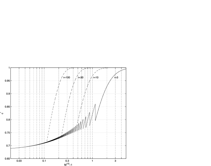
(a)

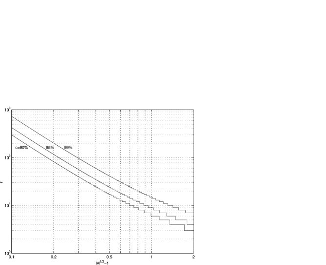
(b)

Figure 1: Behavior of optimum guaranteed confidence as a function of $\sqrt{M}-1$: (a) $c^{*}$ (dashed) and minimum $c^{*}$ (solid); (b) minimum $r$ that guarantees a confidence level.

Given $\mu_{1}$, $\mu_{2}$ and $c$, if the point $(\sqrt{M}-1,c)$ with $M=\mu_{1}\mu_{2}$ lies in the region above the solid curve in Figure 1(a), then there exist values of $r$ for which the estimator (16) globally guarantees the confidence level $c$ for the relative interval defined by $\mu_{1}$ and $\mu_{2}$; the minimum such $r$ is displayed in Figure 1(b). As mentioned earlier, the region referred to in Figure 1(a) (or, equivalently, conditions (17) and (18)) covers most cases of interest. For example, any confidence greater than $85\%$ can be globally guaranteed for any relative interval with $\sqrt{M}-1\leq 1.108$, that is, such that $\mu_{1}\mu_{2}\leq 4.443$.

An important subclass of relative intervals is that for which $\mu_{1}=\mu_{2}=1+m$, $m>0$. An interval of this form corresponds to the requirement that $\hat{p}$ and $p$ do not deviate from each other by a factor greater than $1+m$; the parameter $m$ is thus interpreted as a relative error margin. The guaranteed confidence and required $r$ in this case can be read directly from Figures 1(a) and 1(b), as $\sqrt{M}-1=m$. This particular case is analyzed by Mendo and Hernando (2006; 2008a) for the estimator (2). Comparing Figure 1 of Mendo and Hernando (2008a) with Figure 1(a), the individual (dashed) curves in the latter are seen to be above those in the former (this is most noticeable for small $r$), in accordance with the fact that the estimator (16) is optimum. This yields a reduction in the error margin $m$ for a given $r$ and a desired guaranteed confidence. For example, taking $r=10$, the estimator (2) guarantees a confidence level of $95\%$ for $m=0.9074$, whereas (16) guarantees the same confidence for $m=0.8808$. Furthermore, the latter value is the smallest $m$ for which a confidence level of $95\%$ can be guaranteed by any estimator with the $r$ in question.

As another manifestation of the optimum character of the estimator (16), the curves in Figure 1(b) for $\sqrt{M}-1=m$ are farther to the left than those in Figure 5(a) of Mendo and Hernando (2006). Since, from (5), $\mathrm{E}[N]=r/p$, for certain combinations of $m$ and $c$, this provides a reduction in average observation time to achieve a globally guaranteed confidence $c$ for an error margin $m$. (The fact that the reduction is obtained only for certain combinations of $m$ and $c$ is a consequence of the discrete character of $r$.) Thus, for $m=50\%$, the estimator (2) requires $r=18$ in order to globally guarantee a $90\%$ confidence level, whereas $r=17$ suffices for the estimator (16); furthermore, this is the lowest required $r$ that can be achieved by any estimator.

Comparing the attainable region shown in Figure 1(a), that is, the region above the solid curve, with the corresponding region in Figure 1 of Mendo and Hernando (2008a), they are seen to have similar shape and size, except that for small $m$, the boundary curve is slightly higher in Figure 1(a). Thus, the applicability of the estimator (16) is similar to that of (2) (while achieving better performance).

Another interesting particularization is $\mu_{1}=1+m$, $\mu_{2}=1/(1-m)$, $0<m<1$, which corresponds to requiring that the absolute error $|\hat{p}-p|$ does not exceed a fraction $m$ of the true value $p$. The results for this case can be compared with those of Mendo and Hernando (2008a) and Chen (2007). For $m=40\%$ with a globally guaranteed confidence level of $90\%$, the estimator (2) requires $r=17$ (Mendo and Hernando (2008a), Proposition 1). The results of Chen (2007), Theorem 2, give a sufficient value of $r=46$ for the estimator (3). On the other hand, from Theorem 3, the estimator (16) only requires $r=16$; moreover, it is assured that any other estimator requires at least this $r$ to guarantee (either globally or asymptotically) the same confidence for the $m$ under consideration.

5 Proofs

The following notation is introduced for convenience:

$$\phi(t) = \frac{t^{r-1}\exp(-t)}{(r-1)!},$$ (20)

$$n_{1} = \lceil\Omega/(p\mu_{1})-d\rceil,\qquad n_{2}=\lfloor\Omega\mu_{2}/p-d\rfloor.$$ (21)

Proof of Proposition 1 Let $c_{\mathrm{i}}$ denote $\liminf_{p\rightarrow p_{0}}c(p)$ and assume that $c_{\mathrm{i}}<c_{0}$. For $\varepsilon=(c_{0}-c_{\mathrm{i}})/2$, the definition of limit inferior implies that there exists $p_{\varepsilon}\in(p_{1},p_{2})$ such that $c(p_{\varepsilon})<c_{\mathrm{i}}+\varepsilon<c_{0}$ and thus the estimator does not guarantee the confidence level $c_{0}$ in $(p_{1},p_{2})$. This establishes the result.

Lemma 1

For all $t>0$, the function $\phi$ defined in (20) satisfies

$$0<\phi(t)\leq\frac{(r-1)^{r-1}\exp(-r+1)}{(r-1)!}<1.$$ (22)

[Proof.] The first inequality in (22) is obvious. Let $Q_{r}=(r-1)^{r-1}\exp(-r+1)/(r-1)!.$ Maximizing $\phi(t)$ with respect to $t$, it is seen that $\phi(t)\leq Q_{r}$. Since $Q_{r+1}/Q_{r}=(1+1/(r-1))^{r-1}\exp(-1)<1$ and $Q_{3}=2\exp(-2)<1$, it follows that $Q_{r}<1$ for all $r\geq 3$.

Proof of Proposition 2 Consider $g\in\mathcal{F}_{\mathrm{n}}$ and let $\Omega=\lim_{n\rightarrow\infty}ng(n)$. Given $\varepsilon>0$, there exists $n_{\varepsilon}$ such that $|ng(n)-\Omega|<\varepsilon$ for all $n\geq n_{\varepsilon}$, that is, $(\Omega-\varepsilon)/n<g(n)<(\Omega+\varepsilon)/n.$ Using this, the confidence $c(p)=P[p/\mu_{2}\leq g(N)\leq p\mu_{1}]$ can be bounded for $p\leq(\Omega-\varepsilon)/(\mu_{1}n_{\varepsilon})$ as

$$c(p) \geq P[\lceil(\Omega+\varepsilon)/(p\mu_{1})\rceil\leq N\leq\lfloor(\Omega-\varepsilon)\mu_{2}/p\rfloor],$$ (23)

$$c(p) \leq P[\lceil(\Omega-\varepsilon)/(p\mu_{1})\rceil\leq N\leq\lfloor(\Omega+\varepsilon)\mu_{2}/p\rfloor].$$ (24)

Let $b(n,p;i)$ denote the binomial probability function with parameters $n$ and $p$ evaluated at $i$. From the relationship between binomial and negative binomial distributions, (23) is written as

$$c(p)\geq\sum_{i=0}^{r-1}b\bigl{(}\lceil(\Omega+\varepsilon)/(p\mu_{1})\rceil-1,p;i\bigr{)}-\sum_{i=0}^{r-1}b\bigl{(}\lfloor(\Omega-\varepsilon)\mu_{2}/p\rfloor,p;i\bigr{)}.$$ (25)

According to the Poisson theorem (Papoulis and Pillai (2002), page 113), the right-hand side of (25) converges to $\gamma(r,(\Omega-\varepsilon)\mu_{2})-\gamma(r,(\Omega+\varepsilon)/\mu_{1})$ as $p\rightarrow 0$. This implies that

$$\liminf_{p\rightarrow 0}c(p)\geq\gamma\bigl{(}r,(\Omega-\varepsilon)\mu_{2}\bigr{)}-\gamma\bigl{(}r,(\Omega+\varepsilon)/\mu_{1}\bigr{)}.$$ (26)

Since $\partial\gamma(r,t)/\partial t=\phi(t)$, Lemma 1 establishes that $0<\partial\gamma(r,t)/\partial t<1$. Using this, (26) yields $\liminf_{p\rightarrow 0}c(p)\geq\bar{c}-(\mu_{2}+1/\mu_{1})\varepsilon.$ Taking into account that this holds for all $\varepsilon>0$, it follows that $\liminf_{p\rightarrow 0}c(p)\geq\bar{c}.$ Applying similar arguments to (24) gives $\limsup_{p\rightarrow 0}c(p)\leq\bar{c}.$ Thus, $\lim_{p\rightarrow 0}c(p)$ exists and equals $\bar{c}$.

Lemma 2 ((Abramowitz and Stegun (1970), inequality (4.1.33)))

$t/(1+t)\leq\log(1+t)\leq t$ for $t>-1$, with equality if and only if $t=0$.

Lemma 3

Let $(p_{k})$ be a positive sequence which converges to $0$. For any $\nu_{1}$, $\nu_{2}$ with $\nu_{2}>\nu_{1}>0$, the sequence of functions $(\phi_{k})$ defined as

$$\phi_{k}(\nu)=\frac{(1-p_{k})^{\nu/p_{k}-r}}{(r-1)!}\prod_{i=1}^{r-1}(\nu-ip_{k})$$ (27)

converges uniformly to $\phi(\nu)$, given by (20), in the interval $[\nu_{1},\nu_{2}]$.

[Proof.] Since the sequence $(p_{k})$ is positive and converges to $0$, there exists $k_{1}$ such that $p_{k}<\min\{\nu_{1}/(r-1),1\}$ for $k\geq k_{1}$. Thus, $\phi_{k}(\nu)>0$ for $\nu\in[\nu_{1},\nu_{2}]$, $k\geq k_{1}$ and, therefore,

$$|\phi_{k}(\nu)-\phi(\nu)|=\min\{\phi_{k}(\nu),\phi(\nu)\}\biggl{(}\max\biggl{\{}\frac{\phi_{k}(\nu)}{\phi(\nu)},\frac{\phi(\nu)}{\phi_{k}(\nu)}\biggr{\}}-1\biggr{)}.$$ (28)

Lemma 1 implies that $\min\{\phi_{k}(\nu),\phi(\nu)\}\leq 1$. On the other hand,

$$\max\biggl{\{}\frac{\phi_{k}(\nu)}{\phi(\nu)},\frac{\phi(\nu)}{\phi_{k}(\nu)}\biggr{\}}=\exp\biggl{|}\log\frac{\phi_{k}(\nu)}{\phi(\nu)}\biggr{|}.$$

Substituting into (28), we have

$$|\phi_{k}(\nu)-\phi(\nu)|\leq\exp\biggl{|}\log\frac{\phi_{k}(\nu)}{\phi(\nu)}\biggr{|}-1.$$ (29)

From (20) and (27), it follows that, assuming $\nu\in[\nu_{1},\nu_{2}]$ and $k\geq k_{1}$,

$$\biggl{|}\log\frac{\phi_{k}(\nu)}{\phi(\nu)}\biggr{|}\leq\Biggl{|}\sum_{i=1}^{r-1}\log\biggl{(}1-\frac{ip_{k}}{\nu}\biggr{)}\Biggr{|}+\biggl{|}\biggl{(}\frac{\nu}{p_{k}}-r\biggr{)}\log(1-p_{k})+\nu\biggr{|}.$$ (30)

Using Lemma 2, the first term in the right-hand side of (30) is bounded as follows:

$$\Biggl{|}\sum_{i=1}^{r-1}\log\biggl{(}1-\frac{ip_{k}}{\nu}\biggr{)}\Biggr{|}=-\sum_{i=1}^{r-1}\log\biggl{(}1-\frac{ip_{k}}{\nu}\biggr{)}<\sum_{i=1}^{r-1}\frac{ip_{k}}{\nu-ip_{k}}.$$ (31)

As for the second term, since $\nu\in[\nu_{1},\nu_{2}]$, there exists $k_{2}\geq k_{1}$ such that $p_{k}<\min\{\nu_{1}/r,1\}$ for $k\geq k_{2}$. Thus, $(\nu/p_{k}-r)\log(1-p_{k})<0$, whereas $\nu>0$. From Lemma 2, $-p_{k}/(1-p_{k})<\log(1-p_{k})<-p_{k}$. It follows that

$$\biggl{|}\biggl{(}\frac{\nu}{p_{k}}-r\biggr{)}\log(1-p_{k})+\nu\biggr{|} < \max\biggl{\{}\biggl{|}-\biggl{(}\frac{\nu}{p_{k}}-r\biggr{)}p_{k}+\nu\biggr{|},\biggl{|}-\biggl{(}\frac{\nu}{p_{k}}-r\biggr{)}\frac{p_{k}}{1-p_{k}}+\nu\biggr{|}\biggr{\}}\qquad\hskip 8.0pt$$

$$= \max\biggl{\{}r,\frac{|r-\nu|}{1-p_{k}}\biggr{\}}p_{k}<\max\{r,\nu_{2}\}\frac{p_{k}}{1-p_{k}}.$$

Combining (29)–(5) yields the following bound, valid for all $\nu\in[\nu_{1},\nu_{2}]$, $k\geq k_{2}$:

$$|\phi_{k}(\nu)-\phi(\nu)|<\exp\Biggl{[}\Biggl{(}\sum_{i=1}^{r-1}\frac{i}{\nu-ip_{k}}+\frac{\max\{r,\nu_{2}\}}{1-p_{k}}\Biggr{)}p_{k}\Biggr{]}-1.$$ (33)

The right-hand side of (33) tends to $0$ as $k\rightarrow\infty$. Therefore, $\sup_{\nu\in[\nu_{1},\nu_{2}]}|\phi_{k}(\nu)-\phi(\nu)|$ also tends to $0$, which establishes the result.

Proof of Theorem 1 For $\alpha\in(0,1]$, let the sequence $(p_{k})$, $k\in\mathbb{N}$ be defined as $p_{k}=\alpha M^{-k}$, with $M$ given by (8), and let the sequence of intervals $(I_{k})$ be defined as $I_{k}=(p_{k}/\mu_{2},p_{k}\mu_{1}]$. Consider also the sequence $(f_{k})$, where $f_{k}$ is the probability function of $N$ with parameters $r$ and $p_{k}$. From (5) and (27),

$$f_{k}(n)=p_{k}\phi_{k}(np_{k}).$$ (34)

To facilitate the development, it is convenient to first analyze non-randomized estimators, and then generalize to randomized estimators. Given a non-randomized estimator specified by $g\in\mathcal{F}$, let the sequence of sets $(S_{k})$ be defined such that $n\in S_{k}$ if and only if $g(n)\in I_{k}$. Since the intervals $I_{k}$ are disjoint for different $k$, the sets $S_{k}$ are also disjoint. Let the function $\sigma$ be defined such that $\sigma(n)=k$ if and only if $n\in S_{k}$, with $\sigma(n)=0$ (or an arbitrary negative value) if $n\notin S_{k}$ for all $k\in\mathbb{N}$. Thus, $\sigma$ gives the index $k$ of the interval $I_{k}$ that $g$ associates to each $n$, if any. The function $\sigma$ is determined by $g$; and, for a given $n_{0}$, $\sigma(n_{0})$ can be modified without affecting the rest of values $\sigma(n)$, $n\neq n_{0}$ by adequately choosing $g(n_{0})$.

For the considered non-randomized estimator, let $c_{k}$ denote the probability that $\hat{p}$ lies in $I_{k}$ when $p=p_{k}$, i.e. $c_{k}=\sum_{n\in S_{k}}f_{k}(n)$. Further, let $C(h,H)=\sum_{k=h}^{h+H-1}c_{k}$ for $h$, $H\in\mathbb{N}$ arbitrary. Defining

$$s(n)=\cases{f_{\sigma(n)}(n),&\quad if $n\in S_{h}\cup\cdots\cup S_{h+H-1}$,\cr 0,&\quad otherwise,}$$

the sum $C(h,H)$ can be expressed as $\sum_{n=r}^{\infty}s(n)$. It follows that

$$C(h,H)\leq\sum_{n=r}^{\infty}\max_{k\in\{h,\ldots,h+H-1\}}f_{k}(n),$$ (35)

which holds with equality if the estimator satisfies

$$\sigma(n)=\arg\max_{k\in\{h,\ldots,h+H-1\}}f_{k}(n)\qquad\mbox{for all }n\in\mathbb{N},n\geq r,$$ (36)

where, if the maximum is reached at more than one index $k$, the $\arg\max$ function is arbitrarily defined to give the lowest such index.

As for randomized estimators, consider an arbitrary function $G\in\mathcal{F}_{\mathcal{R}}$, that for each $n$ specifies $\Pi_{n}$, the distribution function of $\hat{p}$ conditioned on $N=n$. Let $I^{\mathrm{c}}=(-\infty,p_{h+H-1}/\mu_{2}]\cup(p_{h}\mu_{1},\infty)$. Conditioned on $N=n$, let $\pi_{n,k}$ and $\pi_{n}^{\mathrm{c}}$ respectively denote the probabilities that $\hat{p}$ is in $I_{k}$ and in $I^{\mathrm{c}}$. Obviously,

$$\pi_{n,h}+\cdots+\pi_{n,h+H-1}+\pi_{n}^{\mathrm{c}}=1.$$ (37)

For $N=n$, the numbers $\pi_{n,h},\ldots,\pi_{n,h+H-1},\pi_{n}^{\mathrm{c}}$ indicate how the conditional probability associated to all possible values of $\hat{p}$ (that is, $1$ in total) is divided among $I_{h}$, …, $I_{h+H-1}$, $I^{\mathrm{c}}$. For a given $n_{0}$, any combination of values $\pi_{n_{0},h},\ldots,\pi_{n_{0},h+H-1},\pi_{n_{0}}^{\mathrm{c}}$ allowed by (37) can be realized, without affecting other values $\pi_{n,k}$, $\pi_{n}^{\mathrm{c}}$ for $n\neq n_{0}$, by adequately choosing the distribution function $\Pi_{n_{0}}$. Defining $c_{k}$ and $C(h,H)$ as in the non-randomized case, the former is expressed as

$$c_{k}=\sum_{n=r}^{\infty}\pi_{n,k}f_{k}(n).$$ (38)

Since all terms in (38) are positive, the series converges absolutely, and thus $C(h,H)$ can be written as

$$C(h,H)=\sum_{k=h}^{h+H-1}c_{k}=\sum_{n=r}^{\infty}\sum_{k=h}^{h+H-1}\pi_{n,k}f_{k}(n).$$

It is evident from this expression that $C(h,H)$ is maximized if, for each $n$, the values $\pi_{n,k}$, $\pi_{n}^{\mathrm{c}}$ are chosen as $\pi_{n,l}=1$ for $l=\arg\max_{k}f_{k}(n)$, $\pi_{n,k}=0$ for $k\neq l$, $\pi_{n}^{\mathrm{c}}=0$; and the resulting maximum coincides with the right-hand side of (35). Thus the inequality (35), initially derived for non-randomized estimators, also holds for the general class of randomized estimators. This implies that for any randomized estimator there exists a non-randomized estimator that attains the same or greater $C(h,H)$.

Let the function $\bar{g}\in\mathcal{F}$ be defined as $\bar{g}(n)=\Omega^{*}/n$, and consider the non-randomized estimator specified by this function. The sets $S_{k}$ and function $\sigma$ associated to this estimator will be denoted as $\bar{S}_{k}$ and $\bar{\sigma}$ respectively. It is seen that

$$\bar{S}_{k}=\bigl{[}\Omega^{*}/(\mu_{1}p_{k}),\Omega^{*}\mu_{2}/p_{k}\bigr{)}\cap\{r,r+1,r+2,\ldots\}.$$ (39)

Let the sequence of functions $(\bar{f}_{k})$ be defined as $\bar{f}_{k}(n)=p_{k}\phi(np_{k}).$ It is readily seen that the equation $\bar{f}_{k}(t)=\bar{f}_{k+1}(t)$ has only one solution, given as $t=\Omega^{*}\mu_{2}/p_{k}$. Similarly, $\bar{f}_{k-1}(t)=\bar{f}_{k}(t)$ has the solution $t=\Omega^{*}/(\mu_{1}p_{k})$. Taking into account that the functions $\bar{f}_{k}$ are unimodal, this implies that $\bar{f}_{k}(n)\geq\bar{f}_{k-1}(n)$ and $\bar{f}_{k}(n)\geq\bar{f}_{k+1}(n)$ for $n\in\bar{S}_{k}$. An analogous argument shows that $\bar{f}_{k}(n)>\bar{f}_{k-i}(n)$ and $\bar{f}_{k}(n)>\bar{f}_{k+i}(n)$ for $n\in\bar{S}_{k}$ and $i\geq 2$. Therefore, the function $\bar{\sigma}$ associated to $\bar{g}$ satisfies a modified version of (36) in which $f_{k}$ is replaced by $\bar{f}_{k}$, that is, $\phi_{k}$ in (34) is replaced by its limit $\phi$. In the following, using the fact that the difference between $\phi_{k}$ and $\phi$ is small for large $k$, the estimator defined by $\bar{g}$ will be used to derive from (35) a more explicit upper bound on $C(h,H)$. Since the sum $C(h,H)$ attained by any estimator is equalled or exceeded by some non-randomized estimator, it will be sufficient to restrict to the class of non-randomized estimators.

Consider an arbitrary non-randomized estimator defined by $g\in\mathcal{F}$ with its corresponding function $\sigma$. Differentiating (5) with respect to $p$, it is seen that $\partial f(n)/\partial p$ is positive for $p<r/n$ and negative for $p>r/n$. According to (39),

$$\Omega^{*}/(\mu_{1}n)\leq p_{k}<\Omega^{*}\mu_{2}/n\qquad\mbox{for }n\in\bar{S}_{k}.$$ (40)

Using Lemma 2, it stems from (9) that

$$\Omega^{*}/\mu_{1}<r<\Omega^{*}\mu_{2}.$$ (41)

The first inequality in (40) and the second in (41) imply that $p_{k-1}=Mp_{k}\geq\Omega^{*}\mu_{2}/n>r/n$ for $n\in\bar{S}_{k}$. Thus $\partial f(n)/\partial p<0$ for $p\geq p_{k-1}$. This implies that $f_{k+i}(n)<f_{k-1}(n)$ for $n\in\bar{S}_{k}$ and $i\leq-2$. It follows that if $\sigma(n_{0})<\bar{\sigma}(n_{0})-1$ for a given $n_{0}$, the sum $C(h,H)$ could be made larger by modifying the value $g(n_{0})$ so as to attain $\sigma(n_{0})=\bar{\sigma}(n_{0})-1$; unless $\sigma(n_{0})=h+H-1$, in which case modifying $g(n_{0})$ cannot make $C(h,H)$ larger. Analogously, the second inequality in (40) and the first in (41) yield $f_{k+i}(n)<f_{k+1}(n)$ for $n\in\bar{S}_{k}$ and $i\geq 2$. Therefore, if $\sigma(n_{0})>\bar{\sigma}(n_{0})+1$ for some $n_{0}$, $C(h,H)$ could be made larger by modifying $g(n_{0})$, unless $\sigma(n_{0})=h$.

According to the above, in order to obtain an upper bound on $C(h,H)$, it suffices to consider non-randomized estimators such that $\sigma(n)\in\{\bar{\sigma}(n)-1,\bar{\sigma}(n),\bar{\sigma}(n)+1\}$ for $n\in\bar{S}_{h}\cup\cdots\cup\bar{S}_{h+H-1}$, $\sigma(n)=h$ for $n<\lceil\Omega^{*}/(\mu_{1}p_{h})\rceil$ and $\sigma(n)=h+H-1$ for $n\geq\lceil\Omega^{*}\mu_{2}/p_{h+H-1}\rceil$. Thus, from (35),

$$C(h,H) \leq \sum_{k=h}^{h+H-1}\sum_{n\in\bar{S}_{k}}\max_{i\in\{-1,0,1\}}f_{k+i}(n)+\sum_{n=r}^{\lceil\Omega^{*}/(\mu_{1}p_{h})\rceil-1}f_{h}(n)$$

$${}+\sum_{n=\lceil\Omega^{*}\mu_{2}/p_{h+H-1}\rceil}^{\infty}f_{h+H-1}(n)$$

$$\leq \sum_{k=h}^{h+H-1}\sum_{n\in\bar{S}_{k}}\max_{i\in\{-1,0,1\}}f_{k+i}(n)+2.$$

Let $\nu_{1}=\Omega^{*}/\mu_{1}$, $\nu_{2}=\Omega^{*}\mu_{2}$, and consider $\varepsilon>0$. From Lemma 3, there exists $k_{1}$ such that $|\phi_{k}(\nu)-\phi(\nu)|<\varepsilon$ for $\nu\in[\nu_{1},\nu_{2}]$, $k\geq k_{1}$. In addition, (39) implies that $np_{k}\in[\nu_{1},\nu_{2}]$ for $n\in\bar{S}_{k}$. From these facts and (34) it stems that $|f_{k}(n)/p_{k}-\phi(np_{k})|<\varepsilon$ for $n\in\bar{S}_{k}$, $k\geq k_{1}$. Thus, for $k\geq k_{1}+1$

$$\max_{i\in\{-1,0,1\}}f_{k+i}(n) < \max_{i\in\{-1,0,1\}}\bigl{[}p_{k+i}\bigl{(}\phi(np_{k+i})+\varepsilon\bigr{)}\bigr{]}$$

$$\leq \max_{i\in\{-1,0,1\}}(p_{k+i}\phi(np_{k+i}))+\varepsilon p_{k-1}.$$

As previously shown, $\bar{f}_{k}(n)=p_{k}\phi(np_{k})$ equals or exceeds $\bar{f}_{k-1}(n)$ and $\bar{f}_{k+1}(n)$ for $n\in\bar{S}_{k}$. Therefore, from (5)

$$\max_{i\in\{-1,0,1\}}f_{k+i}(n)<p_{k}\phi(np_{k})+\varepsilon p_{k-1}.$$ (44)

Substituting (44) into (5),

$$C(h,H)\leq\sum_{k=h}^{h+H-1}\sum_{n\in\bar{S}_{k}}\bigl{(}p_{k}\phi(np_{k})+\varepsilon p_{k-1}\bigr{)}+2.$$ (45)

The number of elements in the set $\bar{S}_{k}$ is less than $\Omega^{*}(\mu_{2}-1/\mu_{1})/p_{k}+1$, according to (39). From (9), this upper bound equals $r\log M/p_{k}+1$. Using this in (45), and taking into account that $p_{k-1}<1$,

$$C(h,H)<\sum_{k=h}^{h+H-1}\sum_{n\in\bar{S}_{k}}p_{k}\phi(np_{k})+\varepsilon H(rM\log M+1)+2.$$ (46)

The term $\sum_{n\in\bar{S}_{k}}p_{k}\phi(np_{k})$ in (46) converges to $\int_{\Omega^{*}/\mu_{1}}^{\Omega^{*}\mu_{2}}\phi(\nu)\,\mathrm{d}\nu=c^{*}$ as $k\rightarrow\infty$. Thus, for the considered $\varepsilon$, there exists $k_{2}$ such that for all $k\geq k_{2}$

$$\biggl{|}\sum_{n\in\bar{S}_{k}}p_{k}\phi(np_{k})-c^{*}\biggr{|}<\varepsilon.$$ (47)

Consequently, defining $k_{0}=\max\{k_{1}+1,k_{2}\}$, inequalities (46) and (47) imply that for all $h\geq k_{0}$, for all $H$, and for $\alpha\in(0,1]$,

$$C(h,H) < H(c^{*}+\varepsilon)+\varepsilon H(rM\log M+1)+2$$

$$= H(c^{*}+\varepsilon P)+2,$$

where $P=rM\log M+2>0$.

Since the minimum of a set cannot be larger than the average of the set, from (5) it follows that there is some $k_{3}\in\{h,\ldots,h+H-1\}$ such that $c_{k_{3}}\leq C(h,H)/H<c^{*}+\varepsilon P+2/H$.

Using the foregoing results, the bound $\liminf_{p\rightarrow 0}c(p)\leq c^{*}$ for an arbitrary estimator can be established by contradiction. Assume that there is some estimator, defined by $G\in\mathcal{F}_{\mathcal{R}}$, such that $\liminf_{p\rightarrow 0}c(p)=c^{*}+d$ with $d>0$. This means that for any $\varepsilon^{\prime}>0$ there exists $p_{0}$ such that $c(p)\geq c^{*}+d-\varepsilon^{\prime}$ for all $p\leq p_{0}$. Thus taking $\varepsilon^{\prime}=d/3$, there is $p_{0}$ such that

$$c(p)\geq c^{*}+2d/3\qquad\mbox{for all }p\leq p_{0}.$$ (49)

On the other hand, taking $\varepsilon=d/(6P)$, $H=\lceil 12/d\rceil$, and with $\alpha\in(0,1]$ arbitrary, the result in the preceding paragraph assures that for any $h$ not smaller than a certain $k_{0}$ (which depends on the considered $\varepsilon$) there exists $k_{3}\in\{h,\ldots,h+H-1\}$ with

$$c_{k_{3}}<c^{*}+\varepsilon P+2/H\leq c^{*}+d/3.$$ (50)

Let $h$ be selected such that $h\geq\max\{k_{0},-\log p_{0}/\log M\}.$ For each $k=h,\ldots,h+H-1$, let $X_{k}$ denote the (possibly empty) set of all points $x\in\mathbb{R}$ such that, for the considered estimator and for $p=p_{k}$, the probability that $\hat{p}$ equals $x$ is at least $d/3$. The number of points in $X_{k}$ cannot exceed $\lfloor 3/d\rfloor$, for otherwise the sum of their probabilities would be greater than $1$. The set $X_{k}$ is determined by $f_{k}$ and $G$ (or by $f_{k}$ and $g$, in the case of a non-randomized estimator defined as $\hat{p}=g(N)$).

Let $\alpha\in(0,1]$ be chosen such that

$$p_{k}/\mu_{2}\notin X_{k}\qquad\mbox{for all }k=h,\ldots,h+H-1.$$ (51)

Such $\alpha$ necessarily exists because (51) excludes only a finite number of possible values from $(0,1]$. This choice of $\alpha$ assures that for $p=p_{k}$, $k=h,\ldots,h+H-1$, the probability that $\hat{p}$ equals $p_{k}/\mu_{2}$ is smaller than $d/3$. Thus $c(p_{k})<c_{k}+d/3$ for $k=h,\ldots,h+H-1$, which, together with (50), gives

$$c(p_{k_{3}})<c^{*}+2d/3.$$ (52)

On the other hand, since $k_{3}\geq h$, from the choice of $h$ it follows that

$$p_{k_{3}}=\alpha M^{-k_{3}}\leq\alpha M^{-h}\leq\alpha M^{\log p_{0}/\log M}=\alpha p_{0}\leq p_{0}.$$

This implies, according to (49), that $c(p_{k_{3}})\geq c^{*}+2d/3$, in contradiction with (52). Therefore $\liminf_{p\rightarrow 0}c(p)\leq c^{*}$.

It has been shown that, for any estimator, $\liminf_{p\rightarrow 0}c(p)$ cannot exceed $c^{*}$. In addition, any non-randomized estimator defined by a function $g\in\mathcal{F}_{\mathrm{n}}$ with $\lim_{n\rightarrow\infty}ng(n)=\Omega^{*}$ achieves $\liminf_{p\rightarrow 0}c(p)=\lim_{p\rightarrow 0}c(p)=c^{*}$. Therefore, $c^{*}$ is the maximum of $\liminf_{p\rightarrow 0}c(p)$ over all randomized or non-randomized estimators.

Proof of Theorem 2 Let $I_{p}(z,w)$ denote the regularized incomplete beta function:

$$I_{p}(z,w) = \frac{1}{B(z,w)}\int_{0}^{p}t^{z-1}(1-t)^{w-1}\,\mathrm{d}t,$$

$$B(z,w) = \int_{0}^{1}t^{z-1}(1-t)^{w-1}\,\mathrm{d}t$$

$$= \frac{\Gamma(z)\Gamma(w)}{\Gamma(z+w)}.$$

From Abramowitz and Stegun (1970), equation (6.6.4), $P[N\leq n]=I_{p}(r,n-r+1)$ for $n\in\mathbb{N}$, $n\geq r$. The confidence for the estimator (12) can thus be written as

$$c(p)=P[n_{1}\leq N\leq n_{2}]=I_{p}(r,n_{2}-r+1)-I_{p}(r,n_{1}-r),$$ (53)

where $n_{1}$ and $n_{2}$ are given by (21) with $\Omega=\Omega^{*}$. It is easy to show that $I_{p}(z,w)$ is an increasing function of $w$ for $w\in\mathbb{R}$. Since $n_{1}<\Omega^{*}/(p\mu_{1})-d+1$ and $n_{2}>\Omega^{*}\mu_{2}/p-d-1$, it follows from (53) that

$$c(p)>\tilde{c}_{2}(p)-\tilde{c}_{1}(p)$$ (54)

with $\tilde{c}_{1}(p)=I_{p}(r,\Omega^{*}/(p\mu_{1})-r-d+1)$ and $\tilde{c}_{2}(p)=I_{p}(r,\Omega^{*}\mu_{2}/p-r-d).$

Expressing $I_{p}(z,w)$ as (Abramowitz and Stegun (1970), equation (26.5.23))

$$I_{p}(z,w) = \frac{{}_{2}F_{1}(z,1-w;z+1;p)p^{z}}{B(z,w)z},$$

$${}_{2}F_{1}(a,b;c;t) = \sum_{j=0}^{\infty}\frac{(a+j-1)^{(j)}(b+j-1)^{(j)}t^{j}}{(c+j-1)^{(j)}j!},$$

the term $\tilde{c}_{2}(p)$ can be written as

$$\tilde{c}_{2}(p) = \frac{1}{B(r,\Omega^{*}\mu_{2}/p-r-d)}\frac{p^{r}}{r}{}_{2}F_{1}(r,r+d+1-\Omega^{*}\mu_{2}/p;r+1;p)$$

$$= \frac{(\Omega^{*}\mu_{2}/p-d-1)^{(r)}}{(r-1)!}\sum_{j=0}^{\infty}\frac{(-1)^{j}(\Omega^{*}\mu_{2}/p-r-d-1)^{(j)}}{(r+j)j!}p^{r+j}$$

$$= \frac{1}{(r-1)!}\sum_{j=0}^{\infty}\frac{(-1)^{j}(\Omega^{*}\mu_{2}-(d+1)p)\cdots(\Omega^{*}\mu_{2}-(d+r+j)p)}{(r+j)j!}.$$ (56)

Similarly,

$$\tilde{c}_{1}(p)=\frac{1}{(r-1)!}\sum_{j=0}^{\infty}\frac{(-1)^{j}(\Omega^{*}/\mu_{1}-dp)\cdots(\Omega^{*}/\mu_{1}-(d+r+j-1)p)}{(r+j)j!}.$$ (57)

According to (5) and (57), both $\tilde{c}_{1}(p)$ and $\tilde{c}_{2}(p)$ can be expressed as power series in $p$: $\tilde{c}_{1}(p)=\sum_{i=0}^{\infty}u_{i}p^{i}$, $\tilde{c}_{2}(p)=\sum_{i=0}^{\infty}v_{i}p^{i}$. Thus, the right-hand side of (54) is also a power series, $\sum_{i=0}^{\infty}w_{i}p^{i}$, with $w_{i}=v_{i}-u_{i}$. The zero-order coefficient is

$$w_{0}=\frac{1}{(r-1)!}\Biggl{(}\sum_{j=0}^{\infty}\frac{(-1)^{j}(\Omega^{*}\mu_{2})^{r+j}}{(r+j)j!}-\sum_{j=0}^{\infty}\frac{(-1)^{j}(\Omega^{*}/\mu_{1})^{r+j}}{(r+j)j!}\Biggr{)}.$$

From the Taylor expansion of $\gamma(r,t)$ (Abramowitz and Stegun (1970), equation (6.5.29)),

$$\gamma(r,t)=\frac{1}{\Gamma(r)}\sum_{j=0}^{\infty}\frac{(-1)^{j}t^{r+j}}{(r+j)j!},$$

the coefficient $w_{0}$ is recognized to be $c^{*}$, reflecting the fact that the difference between the two sides of (54) is vanishingly small as $p\rightarrow 0$. In addition, the first order coefficient $w_{1}$ coincides with the derivative of the right-hand side of (54) evaluated at $p=0$. It follows that $w_{1}>0$ is a sufficient condition for the estimator (12) to asymptotically guarantee the confidence level $c^{*}$.

The coefficient $w_{1}=v_{1}-u_{1}$ is computed as follows. The term $v_{1}$ is obtained from (5) as

$$v_{1}=\frac{1}{(r-1)!}\sum_{j=0}^{\infty}\frac{(-1)^{j+1}(\Omega^{*}\mu_{2})^{r+j-1}[(d+1)+\cdots+(d+r+j)]}{(r+j)j!}.$$ (58)

Substituting $(d+1)+\cdots+(d+r+j)=(r+j)(r+j+1+2d)/2$ into (58) and taking into account that $\exp(t)=\sum_{j=0}^{\infty}t^{j}/j!$, we have

$$v_{1} = \frac{r+1+2d}{2(r-1)!}\sum_{j=0}^{\infty}\frac{(-1)^{j+1}(\Omega^{*}\mu_{2})^{r+j-1}}{j!}+\frac{1}{2(r-1)!}\sum_{j=0}^{\infty}\frac{(-1)^{j}(\Omega^{*}\mu_{2})^{r+j}}{j!}\qquad$$

$$= \frac{(\Omega^{*}\mu_{2})^{r-1}\exp(-\Omega^{*}\mu_{2})}{2(r-1)!}(\Omega^{*}\mu_{2}-r-1-2d).$$

Similarly,

$$u_{1}=\frac{(\Omega^{*}/\mu_{1})^{r-1}\exp(-\Omega^{*}/\mu_{1})}{2(r-1)!}(\Omega^{*}/\mu_{1}-r+1-2d).$$ (60)

From (5) and (60), and making use of (9),

$$w_{1} = \frac{(\Omega^{*}/\mu_{1})^{r-1}}{2(r-1)!}[M^{r-1}\exp(-\Omega^{*}\mu_{2})(\Omega^{*}\mu_{2}-r-1-2d)$$

$$\hphantom{\frac{(\Omega^{*}/\mu_{1})^{r-1}}{2(r-1)!}[}{}-\exp(-\Omega^{*}/\mu_{1})(\Omega^{*}/\mu_{1}-r+1-2d)]$$

$$= \frac{1}{2(r-1)!}\biggl{(}\frac{r\log M}{M-1}\biggr{)}^{r-1}M^{-r/(M-1)}[-(r+1+2d)/M+r-1+2d],$$

which is positive if (13) holds. Thus, (12) asymptotically guarantees the confidence $c^{*}$ for $d$ as in (13).

Lemma 4

For $r$, $n_{0}\in\mathbb{N}$ with $r\geq 3$ and $n_{0}\leq(r-\sqrt{r})/p,$

$$\int_{r}^{n_{0}}t^{r-1}\exp(-pt)\,\mathrm{d}t\geq\sum_{n=r}^{n_{0}-1}(n-1)^{(r-1)}(1-p)^{n-r}.$$ (61)

[Proof.] For $n_{0}$ as given, the sub-integral function in (61) is increasing within the integration range. Consequently, for (61) to hold, it is sufficient that $n^{r-1}\exp(-np)\geq(n-1)^{(r-1)}(1-p)^{n-r}$ for $n=r,\ldots,\lfloor(r-\sqrt{r})/p\rfloor-1$. This condition can be shown to be satisfied by means of reasoning analogous to that in the proof of Lemma 1 of Mendo and Hernando (2008a), part (i). 

Proof of Proposition 3 The confidence for the estimator (14) is expressed as $c_{2}(p)-c_{1}(p)$, $c_{1}(p)=P[N\leq n_{1}-1]$, $c_{2}(p)=P[N\leq n_{2}]$, where $n_{1}$ and $n_{2}$ are given by (21) with $d=1$. Let $c^{\prime}_{2}=1-c_{2}$. A similar argument as in the proof of Proposition 2, based on the Poisson theorem, shows that $\lim_{p\rightarrow 0}c_{1}(p)=\bar{c}_{1}$ and $\lim_{p\rightarrow 0}c^{\prime}_{2}(p)=\bar{c}^{\prime}_{2}$, with $\bar{c}_{1}=\gamma(r,\Omega/\mu_{1})$, $\bar{c}^{\prime}_{2}=1-\gamma(r,\Omega\mu_{2})$. Thus, to establish the desired result, it suffices to prove that $c_{1}(p)<\bar{c}_{1}$ and $c^{\prime}_{2}(p)<\bar{c}^{\prime}_{2}$ for $\mu_{1}$, $\mu_{2}$ as in (15).

Regarding $c^{\prime}_{2}(p)$, it is shown in Appendix C of Mendo and Hernando (2006) that $P[N\leq\lfloor a/p\rfloor]>\lim_{p\rightarrow 0}P[N\leq\lfloor a/p\rfloor]$ for $a>r+\sqrt{r}$. Equivalently, for any $\theta>1$,

$$P\bigl{[}N\geq\bigl{\lfloor}\theta\bigl{(}r+\sqrt{r}\bigr{)}/p\bigr{\rfloor}+1\bigr{]}<\lim_{p\rightarrow 0}P\bigl{[}N\geq\bigl{\lfloor}\theta\bigl{(}r+\sqrt{r}\bigr{)}/p\bigr{\rfloor}+1\bigr{]}.$$

This can be made to correspond to $c^{\prime}_{2}(p)<\bar{c}^{\prime}_{2}$ by taking $\lfloor\Omega\mu_{2}/p-1\rfloor=\lfloor\theta(r+\sqrt{r})/p\rfloor$, that is,

$$\mu_{2}=\frac{\theta(r+\sqrt{r})+p}{\Omega}.$$ (62)

Thus, the inequality $c^{\prime}_{2}(p)<\bar{c}^{\prime}_{2}$ holds if $\mu_{2}$ is given by (62) for some $\theta>1$ or, equivalently, if $\mu_{2}>(r+\sqrt{r}+p)/\Omega$. Therefore, it holds for arbitrary $p$ if $\mu_{2}$ satisfies the second inequality in (15).

As for $c_{1}(p)$, from (5), it can be expressed as

$$c_{1}(p)=\sum_{n=r}^{n_{1}-1}f(n)=\frac{p^{r}}{(r-1)!}\sum_{n=r}^{n_{1}-1}(n-1)^{(r-1)}(1-p)^{n-r}.$$ (63)

According to (21) with $d=1$,

$$n_{1}<\frac{\Omega}{p\mu_{1}}$$ (64)

and thus

$$\bar{c}_{1} = \gamma(r,\Omega/\mu_{1})=\frac{p^{r}}{(r-1)!}\int_{0}^{\Omega/(p\mu_{1})}t^{r-1}\exp(-pt)\,\mathrm{d}t$$

$$> \frac{p^{r}}{(r-1)!}\int_{r}^{n_{1}}t^{r-1}\exp(-pt)\,\mathrm{d}t.$$

From (63), (5) and Lemma 4, it follows that the inequality $c_{1}(p)<\bar{c}_{1}$ is satisfied if

$$n_{1}\leq\frac{r-\sqrt{r}}{p}.$$ (66)

Using (64), it is seen that (66) is fulfilled if $\mu_{1}$ satisfies the first inequality in (15).

Proof of Theorem 3 For $\Omega=\Omega^{*}$, using (8) and (9), the conditions in (15) are written as (17) and (18). The left-hand sides of (17) and (18) are increasing functions of $M$, whereas the right-hand sides decrease with $r$. These inequalities can thus be written as $M\geq h_{1}(r)$, $M\geq h_{2}(r)$, where $h_{1}$, $h_{2}$ are decreasing functions. This proves that for each $r$, one of the inequalities implies the other. Furthermore, defining $h(r)=\min\{h_{1}(r),h_{2}(r)\}$, the allowed range for $M$ is expressed as $M\geq h(r)$ and $h$ is a decreasing function. It only remains to prove that the limiting condition is (17) for $r=\{3,4\}$ and (18) for $r\geq 5$.

The left-hand sides of (17) and (18) are continuous functions of $M>1$. Considering $r$ as if it were a continuous variable, the right-hand sides are also continuous functions. Assume that (17) implies (18) for a given $r_{1}$, that is, that the latter is satisfied when the former holds with equality. Likewise, assume that (18) implies (17) for a given $r_{2}$. The continuity of the involved functions then implies that there exists $t\in[\min\{r_{1},r_{2}\},\max\{r_{1},r_{2}\}]$ such that both (17) and (18) hold with equality for $r=t$, that is,

$$\frac{M-1}{\log M}=\frac{t+\sqrt{t}}{t-1},\qquad\frac{M\log M}{M-1}=\frac{t+\sqrt{t}+1}{t}.$$ (67)

Multiplying both equalities in (67) and substituting into the first yields

$$\log\frac{t+\sqrt{t}+1}{t-\sqrt{t}}-\frac{2\sqrt{t}+1}{t}=0.$$ (68)

It is easily shown that (68) has only one solution, which lies in the interval $(4,5)$. Thus, one of the two conditions (17) and (18) is the limiting one for $r\in\{3,4\}$, whereas the other is for $r=\{5,6,7,\ldots\}$. Taking any value from each set, the limiting condition is seen to be (17) in the former case and (18) in the latter.

References

- Abramowitz and Stegun (1970) Abramowitz, M. and Stegun, I.A., eds. (1970). Handbook of Mathematical Functions, 9th ed. New York: Dover.
- Chen (2007) Chen, X. (2007). Inverse sampling for nonasymptotic sequential estimation of bounded variable means. Available at arXiv:0711.2801v2 [math.ST].
- Haldane (1945) Haldane, J.B.S. (1945). On a method of estimating frequencies. Biometrika 33 222–225. MR0019900
- Lehmann and Casella (1998) Lehmann, E.L. and Casella, G. (1998). Theory of Point Estimation, 2nd ed. New York: Springer. MR1639875
- Mendo and Hernando (2006) Mendo, L. and Hernando, J.M. (2006). A simple sequential stopping rule for Monte Carlo simulation. IEEE Trans. Commun. 54 231–241.
- Mendo and Hernando (2008a) Mendo, L. and Hernando, J.M. (2008a). Improved sequential stopping rule for Monte Carlo simulation. IEEE Trans. Commun. 56 1761–1764.
- Mendo and Hernando (2008b) Mendo, L. and Hernando, J.M. (2008b). Unbiased Monte Carlo estimator with guaranteed confidence. In Proc. IEEE Int. Workshop on Signal Processing Advances in Wireless Communications 625–628. New York: IEEE.
- Mikulski and Smith (1976) Mikulski, P.W. and Smith, P.J. (1976). A variance bound for unbiased estimation in inverse sampling. Biometrika 63 216–217. MR0397965
- Papoulis and Pillai (2002) Papoulis, A. and Pillai, S.U. (2002). Probability, Random Variables and Stochastic Processes, 4th ed. New York: McGraw-Hill.
- Petkovšek et al. (1996) Petkovšek, M., Wilf, H.S. and Zeilberger, D. (1996). . Wellesley: Peters. MR1379802
- Prasad and Sahai (1982) Prasad, G. and Sahai, A. (1982). Sharper variance upper bound for unbiased estimation in inverse sampling. Biometrika 69 286. MR0655698
- Sathe (1977) Sathe, Y.S. (1977). Sharper variance bounds for unbiased estimation in inverse sampling. Biometrika 64 425–426. MR0494647