Chemical Abundances from the Continuum.

Abstract

The calculation of solar absolute fluxes in the near-UV is revisited, discussing in some detail recent updates in theoretical calculations of bound-free opacity from metals. Modest changes in the abundances of elements such as Mg and the iron-peak elements have a significant impact on the atmospheric structure, and therefore self-consistent calculations are necessary. With small adjustments to the solar photospheric composition, we are able to reproduce fairly well the observed solar fluxes between 200 and 270 nm, and between 300 and 420 nm, but find too much absorption in the 270-290 nm window. A comparison between our reference 1D model and a 3D time-dependent hydrodynamical simulation indicates that the continuum flux is only weakly sensitive to 3D effects, with corrections reaching $<10$ % in the near-UV, and $<2$ % in the optical.

1 Introduction

With the exception of stellar effective temperatures, all other atmospheric parameters, including the chemical composition, are typically determined from absorption lines measured in spectra (and see Barklem’s contribution in this volume). The optical and infrared continuum of normal stars is shaped by bound-free and free-free opacity of atomic hydrogen and the ion H^-, but at blue and UV wavelengths several metals become important as continuum absorbers.

In this brief paper, I describe our recent efforts to compile and evaluate the opacity sources relevant for the solar spectrum, and to compute absolute fluxes. Bengt Gustafsson created and actively maintained the opacity data base used in the construction of model atmospheres and spectrum synthesis calculations with MARCS and associated codes (?, ?), and so this contribution is also a tribute to Bengt’s role on making sure the right physical processes are included in the calculation of stellar spectra.

2 Computing absolute stellar fluxes

Two main ingredients are needed for calculating reliable absolute stellar fluxes: accurate opacities and a realistic equation of state. A flexible model atmosphere code is also necessary if we are interested in exploring the impact of varying chemical abundances on the atmospheric structure.

2.1 Opacities

We take our line opacities from the compilations maintained by R. L. Kurucz and distributed through his website. The atomic transition probabilities come from a variety of sources, but Kurucz has obviously made an effort to keep his list updated with reliable laboratory sources. We also made modifications to the linelist adopting Van der Waals damping constants computed by ? when available. Linelists for diatomic molecules are provided by Kurucz for each isotopologue, and we combined them using terrestrial proportions.

Figure 1: Upper panel: individual weighted contribution for each Mg I level to the total photoionization cross section $\sigma=\sum_{i}\sigma_{i}N_{i}/N=\sum_{i}\sigma_{i}g_{i}e^{(-E_{i}/k/T)}$. The total cross-section is shown multiplied by a factor of 10 (dashed line). Lower panel: total weighted cross section from the upper panel, with the abscissae changed from frequency to vacuum wavelengths.

Continuum opacities for C, Mg, Al, Si, and Ca, as computed with the R-matrix method by the Opacity Project, were extracted from TOPBASE (?) and smoothed according to the expected errors in the theoretical energies following ? (see also ?). TOPBASE provides energy levels, radiative transition probabilities, and photoionization cross-sections. The bound-free opacity for all levels should be considered: taking into account only the lowest levels may lead to missing opacity, as illustrated for the case of Mg I in Figure 1. This ion contributes an important part of the opacity in the range 200-300 nm, and the opacity bump at $\sim 280$ nm results from the combined photoionization from a number of levels.

Figure 2: Ratio of the theoretical energies given in TOPBASE with those extracted from the Atomic Spectroscopic Database at NIST for the different states of several ions. The Opacity Project calculations do not consider fine structure, so the energies for different $J$ states are weighted with their degeneracies and averaged.

The computed energies have significant errors, and we correct them to match the energies inferred from wavelengths of lines measured at the laboratory. Figure 2 shows the ratio of the energies from TOPBASE and those from the atomic database at the US National Institute for Standards and Technology (NIST) for several ions. The errors are small in some cases, but in others can reach up to 20%.

The Opacity Project calculations have been extended to heavier ions as part of the Iron Project (see ?, ?). With help from the scientists involved in the calculations, I have translated the data to the same format used in TOPBASE, building new model atoms (including continuous opacities) for neutral and ionized iron. These are also used here.

2.2 Equation of state

The relationship among the main thermodynamical quantities needs to be properly computed according to the chosen chemical composition. We adopt the temperatures and densities from a model atmosphere, and then solve the equations of chemical equilibrium for all species, including molecules, deriving a consistent electron density.

For this purpose we use the code Synspec (?), with a number of recent upgrades. A suite of subroutines to solve the molecular equilibrium have been adopted (I. Hubeny, private communication), and the partition functions for both atoms and molecules are now from the data of ? (and also private comm. from Irwin). The 1D version of the code ass$\epsilon$t (?) was used to solve the radiative transfer equation.

2.3 Model atmosphere code

A model atmosphere is paramount in order to compute stellar fluxes. In order to check whether there is feedback to the atmospheric structure from changes in the chemical composition, we also need a model atmosphere code. We have adopted the linux port of Kurucz’s Atlas9, recently published by ?. To facilitate multiple calculations, I wrote a set of scripts that prepare the input to the code, check for convergence, and adjust the number of iterations accordingly.

2.4 The Players

Several elements are important when considering absolute fluxes for a solar-like star. Carbon and oxygen do not provide significant continuous opacity, but form molecules (mainly CH, OH, CO) with transitions that block the radiation in some specific regions. Magnesium, aluminum, silicon and iron atoms provide genuine bound-free absorption, while others such as Ca and Na contribute only indirectly to the opacity, donating electrons which may bound with hydrogen to form H^-, or shifting the iron ionization balance. Finally, if the abundance of helium is increased at the expense of hydrogen, it will indirectly reduce the H and H^- opacities.

3 Taking a shortcut

One might naively imagine that the feedback from modest perturbations in the metal abundances to the atmospheric structure would be minor. As it is usually done for the analysis of lines, I computed the variations in the emerging fluxes for a solar-like model associated with changes of $+0.2$ dex in the abundances of He, C, O, Mg, and Fe. This exercise was described at another conference (?). As expected, the UV flux was reduced when the abundances of C, O, Mg, or Fe were enhanced, but a large flux increase was noticed when the ratio He/H was increased.

Figure 3: Changes in the emergent fluxes as a result of an increase in the abundances of helium (top panel), all metals (central panel), and magnesium (bottom panel). The results obtained when the composition of the model atmosphere is changed consistently with that adopted for the equation of state and spectral synthesis correspond to the dashed lines. The results from the calculations using a fixed atmospheric structure (solid lines) overestimate the flux changes.

This approximation was of course of dubious validity, in particular for such an abundant element as helium. New calculations in which the composition of the model atmosphere is changed consistently show that the changes in the fluxes were systematically overestimated: the atmospheric structure adjusts in response to changes in the abundances and the variations in the emerging fluxes are much smaller than initially predicted. The original calculations for enhancements of 0.2 dex in the abundances of He, Mg, and the overall metallicity are shown with solid lines in Figure 3, while the new calculations with consistent structures are shown with dashed lines. The large correction for helium is not a big surprise, but the flux variations are also reduced significantly for the case of Mg, which only contributes continuum opacity in a limited spectral window. Note that for the self-consistent calculations the changes in the flux at some wavelengths are compensated at others in order to maintain the effective temperature constant.

4 A test with solar observations

As an exercise, we computed a grid changing the abundances of all metals, as well as C/H, O/H, and Mg/H, from the reference values by plus and minus 0.2 dex, and then used interpolation to fit solar observations. For consistency, the reference abundances were those recently used by Kurucz for his NEW opacity distribution functions and models (?): $\log{\rm N(X)/N(H)}+12=8.52,8.83,7.58$ and $7.50$ with X replaced by C, O, Mg, and Fe, respectively. For the solar observations we used an average of SOLSTICE and SUSIM spectra, as discussed by ?, with a resolution of about 3 Å.

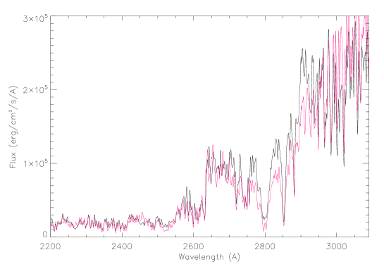
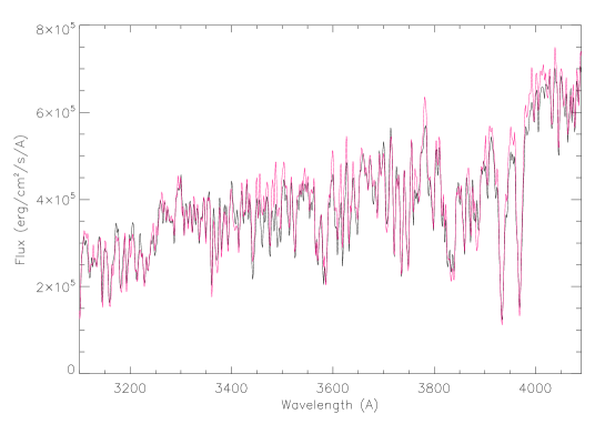
Figure 4: Average observed solar spectrum (black, see text) and best-fitting model after adjusting the abundances of C, O, Mg, and all metals together (red).

Figure 4 shows the best-fitting solution, which corresponds to changes from the reference abundances of $-0.18$ dex in overall metallicity (all metals), and of $+0.12$, $+0.07$, and $+0.12$ dex in C, O and Mg. There is a fair match of the observations for wavelengths between 200-270 nm, and a good match is achieved in the 300-400 nm window, but too much opacity is predicted in the region around the Mg II resonance lines. Given that we have not varied the abundances of important electron donors such as Na, Ca and Si, these results must be considered preliminary.

5 ‘Three-dimensional’ effects

The introduction of 3D hydrodynamical simulations in the analysis of the solar spectrum has showed that corrections to the derived abundances from atomic lines tend to be small, while molecular lines are overall more sensitive to temperature inhomogeneities. The continuum at about 300 nm is formed in deep photospheric regions, but as the opacity increases towards shorter wavelengths the continuum formation is rapidly shifted to higher layers, where inhomogeneities may have a larger impact on line formation.

Ass$\epsilon$t, a new 3D radiative transfer code capable of handling arbitrarily complex opacities, has been recently introduced by ?. Computing the entire spectrum for a series of 3D snapshots sampling the spectrum fast enough to avoid missing line opacity requires a large investment of computing time, even on a modern supercomputer. Nonetheless, we can explore if there are any effects on the continuum by using only a few hundred frequencies.

Figure 5: Comparison of the continuum fluxes for our reference 1D (dashed line) and 3D (solid line; including H lines) models. The 1$\sigma$ range for the 100 snapshots from the 3D simulation are also shown with dotted lines.

Figure 5 shows the comparison between the computed continuum flux (including Balmer lines) for the 3D simulation of ? and our reference solar 1D Kurucz model. For these spectral synthesis calculations the same opacities, and equation of state were used, accounting properly for Rayleigh (atomic H) and electron scattering, which anyhow makes a negligible difference in this case. The fluxes predicted for the 3D model (the average of 100 snapshots covering nearly an hour of solar time; solid line) are similar to those for the 1D model (dashed line), with the difference amounting to about 5–10 % at maximum in the 200-300 nm window, and $<2$ % in the optical and near-infrared.

6 Conclusions

We compile the main sources of opacity in the solar photosphere and compute absolute fluxes based on classical one-dimensional LTE model atmospheres. Metal absorption provides an important contribution to the near UV opacity, and the photoionization cross-sections of many levels need to be considered. The energies predicted by the R-matrix calculations performed within the Opacity Project for some ions have uncertainties of up to 20 %, and therefore it is recommended to use the observed energies instead.

Small changes in the abundances of He, Mg and the iron-peak elements can have an important feedback on the atmospheric structure, and thus consistent calculations are needed to obtain the correct results. With modest adjustments to the standard photospheric abundances, we find it possible to reproduce fairly well the observed solar fluxes between 200-270 nm and even better in the range 300-410 nm, while too much absorption is found in the window 270-290 nm. This may hint at excessive Mg bound-free absorption, although further tests are necessary.

We compare the continuum fluxes computed with our reference 1D model with those from a 3D time-dependent radiative-hydrodynamical simulation and found limited changes, reaching up to 10 % in the near-UV.

References

References

- [1]
- [2] [] Allende Prieto C 2007 ArXiv e-prints 709.
- [3]
- [4] [] Allende Prieto C, Hubeny I & Lambert D L 2003 ApJ 591, 1192–1202.
- [5]
- [6] [] Allende Prieto C, Lambert D L, Hubeny I & Lanz T 2003 ApJS 147, 363–368.
- [7]
- [8] [] Asplund M, Nordlund Å, Trampedach R, Allende Prieto C & Stein R F 2000 A&A 359, 729–742.
- [9]
- [10] [] Barklem P S, Piskunov N & O’Mara B J 2000 A&AS 142, 467–473.
- [11]
- [12] [] Bautista M A 1997 A&AS 122, 167–176.
- [13]
- [14] [] Bautista M A, Romano P & Pradhan A K 1998 ApJS 118, 259–265.
- [15]
- [16] [] Cunto W, Mendoza C, Ochsenbein F & Zeippen C J 1993 Bulletin d’Information du Centre de Donnees Stellaires 42, 39–+.
- [17]
- [18] [] Grevesse N & Sauval A J 1998 Space Science Reviews 85, 161–174.
- [19]
- [20] [] Gustafsson B, Edvardsson B, Eriksson K, Graae Jorgensen U, Nordlund A & Plez B 2008 ArXiv e-prints 805.
- [21]
- [22] [] Hubeny I & Lanz T 2000 0, 0.
- [23]
- [24] [] Irwin A W 1981 ApJS 45, 621–633.
- [25]
- [26] [] Jørgensen U G & Gustafsson B 1994 Astronomy and Astrophysics Review 6, 19–65.
- [27]
- [28] [] Koesterke L, Allende Prieto C & Lambert D L 2008 ApJ 680, 764–773.
- [29]
- [30] [] Nahar S N 1995 A&A 293, 967–977.
- [31]
- [32] [] Sbordone L, Bonifacio P & Castelli F 2007 in F Kupka, I Roxburgh & K Chan, eds, ‘IAU Symposium’ Vol. 239 of IAU Symposium pp. 71–73.
- [33]