Department of Physics Doctor of Philosophy in Physics May 2008 May 2008

Edward H. FarhiProfessor of Physics

Thomas J. GreytakProfessor of Physics

Quantum Computation Beyond the Circuit Model

The quantum circuit model is the most widely used model of quantum computation. It provides both a framework for formulating quantum algorithms and an architecture for the physical construction of quantum computers. However, several other models of quantum computation exist which provide useful alternative frameworks for both discovering new quantum algorithms and devising new physical implementations of quantum computers. In this thesis, I first present necessary background material for a general physics audience and discuss existing models of quantum computation. Then, I present three new results relating to various models of quantum computation: a scheme for improving the intrinsic fault tolerance of adiabatic quantum computers using quantum error detecting codes, a proof that a certain problem of estimating Jones polynomials is complete for the one clean qubit complexity class, and a generalization of perturbative gadgets which allows $k$-body interactions to be directly simulated using 2-body interactions. Lastly, I discuss general principles regarding quantum computation that I learned in the course of my research, and using these principles I propose directions for future research.

Chapter 1 Introduction

1.1 Classical Computation Preliminaries

This thesis is about quantum algorithms, complexity, and models of quantum computation. In order to discuss these topics it is necessary to use notations and concepts from classical computer science, which I define in this section.

The “big-O” family of notations greatly aids in analyzing both classical and quantum algorithms without getting mired in minor details. Although it may seem like a trivial notation, it is the first step in a chain of increasing abstraction which allows computer scientists to analyze the general laws of computation which apply whether the computer is using base 2 or base 20, and whether it is made of transistors or tinker toys. By following this chain we will reach the major open questions about complexity classes and their relations to one another. The big-O notation is defined as follows.

Definition 1.

Given two functions $f(n)$ and $g(n)$, $f(n)$ is $O(g(n))$ if there exist constants $n_{0}$ and $c>0$ such that $|f(n)|<c|g(n)|$ for all $n>n_{0}$.

Definition 2.

Given two functions $f(n)$ and $g(n)$, $f(n)$ is $\Omega(g(n))$ if there exist constants $n_{0}$ and $c>0$ such that $|f(n)|>c|g(n)|$ for all $n>n_{0}$.

Definition 3.

Given two functions $f(n)$ and $g(n)$, $f(n)$ is $\Theta(g(n))$ if it is $O(g(n))$ and $\Omega(g(n))$.

Thus, $O$ describes upper bounds, $\Omega$ describes lower bounds, and $\Theta$ describes asymptotic behavior modulo an overall multiplicative constant. The standard way to describe the efficiency of an algorithm is to use “big-O” notation to describe the number of computational steps the algorithm uses to solve a problem as a function of number of bits of input. For example, the standard method for multiplying two $n$-digit numbers that is taught in elementary school uses $\Theta(n^{2})$ elementary operations in which individual digits are manipulated. By using big-O notation we can avoid distinguishing between $2n^{2}$ and $50n^{2}$ which allows us to disregard unnecessary details.

Moving one level higher in abstraction, we reach computational complexity classes. These are sets of problems solvable with a given set of computational resources. For example, the complexity class P is the set of problems solvable on a Turing machine in a number of steps which scales polynomially in the number of bits of input $n$, that is, with $O(n^{c})$ steps for some constant $c$. Note that for a problem to be contained in P, all problem instances of size $n$ must be solvable in time $\mathrm{poly}(n)$, including highly atypical worst-case instances.

Complexity classes are usually defined in terms of decision problems. These are problems that admit a yes/no answer, such as the problem of determining whether a given integer is prime. Many problems are not of this form. For example, the problem of factoring integers has an output which is a list of prime factors. However, it turns out that in almost all cases, problems can be reduced with polynomial overhead to decision versions. For example, consider the problem where, given two numbers $a$ and $b$, you are asked to answer whether $a$ has a prime factor smaller than $b$. Given a polynomial time algorithm solving this problem, one can construct a polynomial time algorithm for factoring using this algorithm as a subroutine Thus by considering only decision problems (or more technically, the associated languages), complexity theorists are simplifying things without losing anything essential. Because problems are usually equivalently hard to their decision versions, we will often gloss over the distinction between the problems and their decision versions in this thesis.

Some complexity classes describe models of computation which are essentially realistic. P describes problems solvable in polynomial time on Turing machines. Until recently, every plausible deterministic model of universal computation has led to the same set of problems solvable in polynomial time. That is, all models of universal computation could be simulated with polynomial overhead by a Turing machine, and vice versa. Thus the complexity class P was regarded as a robust description of what could be efficiently computed deterministically in the real world, which captures something fundamental and is not just an artifact of the particular model of computation being studied.

For example, in the standard formulation of a Turing machine, each location on the tape can take two states. That is, it contains a bit. If you instead allow $d$ states (a “dit”) then the speedup is only by a constant factor, which already disappears from our notice when we use big-O notation. Furthermore, even parallel computation, although useful in practice, does not generate a complexity class distinct from P, provided one allows at most polynomially many processors as a function of problem size.

One may ask why polynomial time is chosen as the definition of efficiency. Certainly it would be a stretch to consider an algorithm operating in time $n^{25}$ efficient, or an algorithm operating in time $2^{\lceil 0.0001\sqrt{n}\rceil}$ inefficient. There are several reasons for using polynomial time as a mathematical formalization of efficiency. First of all, it is mathematically convenient. It is a robust definition which allows one to ignore many details of the implementation. Furthermore, asymptotic complexity is more robust than the complexity of small instances, which can be influenced by the presence of lookup tables or other preprocessed information hidden in the program. Secondly, it appears to do a good job of sorting the efficient algorithms from the inefficient algorithms in practice. It is rare to obtain a polynomial time classical algorithm with runtime substantially greater than $n^{3}$ or a superpolynomial time algorithm with runtime substantially less than $2^{n}$. Furthermore, whenever polynomial time algorithms are found with large exponents, it usually turns out that either the runtime in practice is much better than the worst case theoretical runtime, or a more efficient algorithm is subsequently found.

Sometimes a problem not known to be in P seems to be efficiently solvable in practice. This can happen either because the problem is not in P but the worst case instances are hard to construct, or because the problem actually is in P but the proof of this fact is difficult. Linear programming provides an interesting and historically important example of the latter. For this problem the best known algorithm was for a long time the simplex method, which had exponential worst-case complexity, but was generally quite efficient in practice. An algorithm with polynomial time worst-case complexity has since been discovered.

One can also consider probabilistic computation. That is, one can give the computer the ability to generate random bits, and demand only that it give the correct answer to a problem with high probability. It is clear that the set of problems solvable in this way contains P and possibly goes beyond it. The standard formalization of this notion is the complexity class BPP, which is defined as the set of decision problems solvable on a probabilistic Turing machine with probability at least $2/3$ of giving the correct answer. (BPP stands for Bounded-error Probabilistic Polynomial-time.) Note that, like P, BPP is defined using worst-case instances. The probabilities appear not by randomizing over problem instances, but by randomizing over the random bits used in the probabilistic algorithm. The probability $2/3$ appearing in the definition of BPP may appear arbitrary, and in addition, not very high. However, choosing any other fixed probability strictly between $1/2$ and $1$ yields the same complexity class. This is because one can amplify the success probability arbitrarily by running the algorithm multiple times and taking the majority vote.

Prior to the discovery of quantum computation, no plausible model of computation was known which led to a larger complexity class than BPP. Just as all plausible models of classical deterministic computation turned out to be equivalent up to polynomial overhead, the same was true for classical probabilistic computation. Furthermore, it is now generally suspected that BPP=P. In practice, randomized algorithms usually work just fine if the random bits are replaced by pseudorandom bits, which although generated by deterministic algorithms, pass most naive tests of randomness (e.g. the various means and correlations come out as one would expect for random bits, obvious periodicities are absent, and so forth). The conjecture that P=BPP is currently unproven, and finding a proof is a major open problem in computer science. (Until recently, the problem of primality testing was known to be in BPP but not P, increasing the plausibility that the classes are distinct. However, a deterministic polynomial-time algorithm for this problem was recently discovered.) The notion that BPP captures the power of polynomial time computation in the real world was eventually formalized as the strong Church-Turing thesis, which states:

Any “reasonable” model of computation can be efficiently simulated on a probabilistic Turing machine.

If BPP=P then dropping the word “probabilistic” results in an equivalent claim. The strong Church-Turing thesis is named in reference to the original Church-Turing thesis, which states

Any “reasonable” model of computation can be simulated on a Turing machine.

The original Church-Turing thesis is a statement only about what is computable and what is not computable, where no limit is made on the amount of time or memory which can be used. Thus we have reached a very high level of abstraction at which runtime and memory requirements are ignored completely. It is perhaps not intuitively obvious that with unlimited resources there is anything one cannot compute. The fact that uncomputable functions exist was a profound realization with an simple proof. One can see by Cantor diagonalization that the set of all decision problems, i.e. the set of all maps from bitstrings to $\{0,1\}$, is uncountably infinite. In contrast, the set of all computer programs, which can be represented as bitstrings, is only countably infinite. Thus, computable functions make up an infinitely sparse subset of all functions.

This leaves the question of whether one can find a natural function which is uncomputable. In 1936, Alan Turing showed that the problem of deciding whether a given program terminates is undecidable. This can be proven by the following simple reductio ad absurdum. Suppose you had a program $A$, which takes two inputs, a program, and the data on which the program is to act. $A$ then answers whether the given program halts when run on the given data. One could use $A$ as a subroutine to construct another program $B$ that takes a single input, a program. $B$ determines whether the program halts when given itself as the data. If the answer is yes, then $B$ jumps into an infinite loop, and if the answer is no then $B$ halts. By operating $B$ on itself one thus arrives at a contradiction.

As we shall see in section 1.3, quantum computers provide the first significant challenge to the strong Church-Turing thesis. In general, it is difficult to prove that one model of computation is stronger than another. By discovering an algorithm, one can show that a given model of computation can solve a certain problem with a certain number of computational steps. However, in most cases it is not known how to show that no efficient algorithm on a given model of computation exists for a given problem. In 1994, Peter Shor discovered a quantum algorithm which can factor any $n$-bit number in $O(n^{3})$ time[160]. There is no proof that this problem cannot be solved in polynomial time by a classical computer. However, no polynomial time classical algorithm for factoring has ever been discovered, despite being studied since at least 200BC (cf. sieve of Eratosthenes). Furthermore, factoring has been well-studied in modern times because a polynomial time algorithm for factoring would allow the decryption of the RSA public key cryptosystem, which is used ubiquitously for electronic transactions. The fact that quantum computers can factor efficiently and classical computers can’t is one of the strongest pieces of evidence that quantum computers are more powerful than classical computers.

A second piece of evidence for the power of quantum computers is that quantum algorithms are known which can efficiently simulate the time evolution of many-body quantum systems, a task which classical computers apparently cannot perform despite decades of effort along these lines. The search for polynomial time classical algorithms to simulate quantum systems has been intense because they would have large economic and scientific impact. For example, they would greatly aid in the design of new materials and medicines, and could aid in the understanding of mysterious condensed-matter systems, such as high-temperature superconductors.

Quantum computers do not provide a challenge to the original Church-Turing thesis. As we shall see in section 1.2, the behavior of a quantum computer can be completely predicted by muliplying together a series of exponentially large unitary matrices. Thus any problem solvable on a quantum computer in polynomial time is solvable on a classical computer in exponential time. Hence quantum computers cannot solve problems such as the halting problem.

Other complexity classes relating to realistic classical models of computation have been defined. (See [141] for overview.) These are weaker than BPP. The most important of these for the purposes of this thesis are L and NC1. L stands for Logarithmic space, and NC stands for Nick’s Class. L is the set of problems solvable using only logarithmic memory (other than the memory used to store the input). The class NC1 is the set of problems solvable using classical circuits of logarithmic depth. Similarly, NC2 is the set of problems solvable in depth $O(\log^{2}(n))$, and so on. Roughly speaking, NC1 can be identified as those problems in P which are highly parallelizable. For a detailed explanation of why this is a reasonable intepretation of this complexity class see [141]. For an illustration of the meaning of circuit depth see figure 1.1.

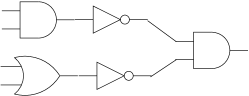
Figure 1.1: The most common way to measure the complexity of a circuit is the number of gates, in this case five. However, one can also measure the depth. In this example, the circuit is three layers deep. The number of gates corresponds to the number of steps in the corresponding sequential algorithm. The depth corresponds to the number of steps in the corresponding parallel algorithm, since gates within the same layer can be performed in parallel.

I have described NC1 using logic circuits. The classical complexity classes such as P and BPP can also be defined using logic circuits such as the one shown in figure 1.1. A given circuit takes a fixed number of bits of input (four in the circuit of figure 1.1). Thus, an algorithm for a given problem corresponds to an infinite family of circuits, one for each input size. It is tempting to suggest that P consists of exactly those problems which can be solved by a family of circuits in which the number of gates scales polynomially with the input size. However, this is not quite correct. The problem is that we have not specified how the circuits will be generated. It is unreasonable to specify an algorithm by an infinitely long description containing the circuit for each possible input size. Such arbitrary families of circuits are called “nonuniform”.

The set of problems solvable by polynomial size nonuniform circuits may be much larger than P, because one can precompute the answers to the problem and hide them in the circuits. One can even “solve” uncomputable problems this way. A uniform family of circuits is one such that given an input size $n$, one can efficiently generate a description of the corresponding circuit. One may for example demand that a fixed Turing machine can produce a description of the circuit corresponding to $n$, given $n$ as an input. In practice, a family of circuits is usually described informally, such that it is easily apparent that it is uniform. The set of decision problems efficiently solvable by a uniform family of polynomial size circuits is exactly P.

While discussing circuits, it bears mentioning that the set of gates used in figure 1.1, namely AND, OR, and NOT, are universal. That is, any function from $n$ bits to one bit (here we are again restricting to decision problems out of convenience and not necessity) can be computed using some circuit constructed from these elements. The proof of this is fairly easy, and the interested reader may work it out independently. A solution is given in appendix A. Note that the number of possible functions from $n$ bits to one bit is $2^{2^{n}}$. In contrast the number of possible circuits with $n$ gates is singly exponential in $n$. Thus, most of the functions on $n$ bits must have exponentially large circuits. Both this universality result and this counting argument have quantum analogues, which are discussed in subsequent sections.

For this thesis, P, BPP, L, and NC1 are a sufficient set of realistic classical complexity classes to be familiar with. We’ll now move on to describe a few of the more fanciful classes. These describe models of computation which are not realistic and classes of problems not necessarily expected to be efficiently solvable in the real world. The most important of these is NP. NP stands for Nondeterministic Polynomial-time. Loosely speaking, it is the set of problems whose solutions are verifiable in polynomial time. NP contains P, because if you have a polynomial time algorithm for correctly solving a problem, you can always verify a proposed solution in polynomial time by simply computing the solution yourself.

More precisely, NP is defined in terms of witnesses (also sometimes called proofs or certificates). These are simply bitstrings which certify the correctness of an answer to a given problem. NP is the set of decision problems such that there exists a polynomial time algorithm (called the verifier), such that if the answer to the instance is yes, there exist a biststring of polynomial length (the witness), which the verifier accepts. If the answer to the instance is no, then the verifier will reject all inputs. This definition can be illustrated using Boolean satisfiability, which is a cannonical example of a problem in NP. The problem of Boolean satisfiability is, given a Boolean formula on $n$ variables, determine whether there is some assignment of true/false to these variables which makes the Boolean formula true. The witness in this case is a string of $n$ bits listing the true/false values of each of the variables. The verifier simply has to substitute these values in and evaluate the Boolean formula, a task easily doable in polynomial time.

NP apparently does not correspond to the set of problems efficiently solvable using any realistic model of computation. Why then would anyone study NP? One reason is that, although there is clearly more practical interest in understanding which problems are efficiently solvable, there is certainly some appeal at least philosophically, in knowing which problems have efficiently verifiable solutions. Perhaps the most important motivation, however, is that by introducing a strange model of computation such as nondeterministic Turing machines, we gain a tool for classifying the difficulty of computational problems.

When faced with a difficult computational problem, it is very difficult to know whether one’s inability to find an efficient algorithm is fundamental or merely a failure of imagination. How can one know whether it is time to give up, or whether the solution around the next corner? Complexity classes give us two handles on the difficulty of a computational problem: containment and hardness. Containment is the more straightforward of the two. If a problem is contained in a given complexity class, then it can be solved by the corresponding model of computation. In a sense this gives an upper bound on the problem’s difficulty. The less obvious concept is hardness. In computer science, “hardness” is a technical term with a precise meaning different from its common usage. If a problem is hard for a given complexity class, this means that any problem in that class is reducible to an instance of that problem. For example, if a problem is NP-hard, it means that any problem contained in NP can be reduced to an instance of that problem in polynomial time and with at most polynomial increase in problem size. Thus, up to polynomial factors, an NP-hard problem is at least as hard as any problem in NP. If one could solve that problem in polynomial time, then one could solve all NP problems in polynomial time.

It not obvious that NP-hard problems exist. After all, how could one ever show that every single problem in NP reduces to a given problem? We don’t even know what all the problems in NP are! We’ll use Boolean satisfiability as an example to see how it is in fact possible to prove that a problem is NP-hard. As discussed earlier, logic circuits made from AND, OR, and NOT gates form a universal model of computation, equal in power (up to polynomial factors) to the Turing machine model. (See appendix A.) Thus the verifier for a problem in NP can be constructed as a logic circuit from such gates. Such a logic circuit corresponds directly to a Boolean formula made from AND, OR, and NOT. This formula will be satisfiable if and only if there exists some input (the witness) which causes the verifier to accept. Thus we have proven that Boolean satisfiability is NP-hard. Given this fact, one can then prove the NP-hardness of other problems by reductions of Boolean satisfiability to other problems. Boolean satisfiability has the property that it is both contained in NP and it is NP-hard. Such problems are called NP-complete. In a well-defined sense, NP-complete problems are the hardest problems in NP. Furthermore, if one specifies a problem and says it is complete for class X, then that statement uniquely defines complexity class X.

Boolean satisfiability is not the only NP-complete problem. In fact, there are now hundreds of NP-complete problems known. (See [76] for a partial catalog of these.) Remarkably, experience has shown that if a well-defined computational problem resists all attempts to find polynomial time classical solution, it almost always turns out to be NP-hard. There are only a few problems currently known which are believed to be neither in P nor NP-hard. These include factoring, discrete logarithm, graph isomorphism, and approximating the shortest vector in a lattice. If a problem is NP-hard, this is taken as evidence that the problem is not solvable in polynomial time. If it were, then all of NP would be solvable in polynomial time. This is considered unlikely, becaue it seems contrary to experience that verifying the solution to a problem is fundamentally no harder than finding the solution. Furthermore, it seems unlikely that all those hundreds of NP-complete problems really do have polynomial-time solutions which were never discovered despite tremendous effort by very smart people over long periods of time. On the other hand, there is no proof that all of NP is not solvable in polynomial time. This is the famous P vs. NP problem which, for various reasons is thought to be very difficult.

NP is not the only complexity class based on a non-realistic model of computation. Another important class is coNP. This is the set of problems which have witnesses for the no instances. In other words, these problems are the complements of the problems in NP. NP and coNP overlap but are believed to be distinct. The problem of factoring integers is known to be contained in both NP and coNP. This is one reason factoring is not believed to be NP-complete. If it were then NP would be contained in coNP. Graph isomorphism is also suspected to be contained in the intersection of NP and coNP. MA is the probabilistic version of NP, where the verifier is a BPP machine rather than a P machine. PSPACE is the set of problems solvable using polynomial memory. Polynomial space is a very powerful model of computation. The class PSPACE contains both NP and coNP and is believed to be strictly larger than either. #P is like NP except to answer a #P problem one must count the number of witnesses rather than just answering whether any witnesses exist. #P is therefore not a decision class. To make comparisons between #P and decision classes one often uses $P^{\#P}$, which is the set of problems solvable by a polynomial time machine with access to an “oracle” which at any timestep can be queried to solve a #P problem. Many more complexity classes have been defined (see [1]). However the ones described above will suffice for this thesis.

As is apparent from the preceeding discussion, many complexity-theoretic results are founded on widely accepted conjectures, such as the conjecture that P is not equal to NP. This is perhaps an unfamiliar situation. These conjectures are neither proven mathematical facts, nor are they the familiar sort of empirical facts based on physical experiments. They are instead empirical facts based on mathematical evidence. How can one assign probability of correctness to mathematical conjectures? Does it even make sense to do so? These are interesting philosophical questions, but to my knowledge unresolved ones. In any case, they are beyond the scope of this thesis. In practice the conjecture that P is not equal to NP is almost universally believed by the relevant experts. Many other similar complexity-theoretic conjectures are often also considered be well-founded, although not necessarily as much so as P $\neq$ NP.

In the presence of all this conjecturing, it is worth mentioning that some relationships between complexity classes are known with certainty. One thing that is known in general is that the class defined by a space bound of $n$ is contained in the class defined by a time bound of $2^{n}$. This is because any algorithm running for time longer than $2^{n}$ with only $n$ bits of memory necessarily revisits a state it has already been in, and is therefore in an infinite loop. Thus any problem solvable in logarithmic space is solvable in polynomial time, and any problem solvable in polynomial space is solvable in exponential time. In general, containments are easier to prove the separations. For example, it is trivial to show that P is contained in NP, but nobody has ever succeeded in showing that NP is larger than P. An exception to this is that separations are not hard to prove between classes of the same type. For example, it is proven that exponential time (EXP) is a strictly larger class than polynomial time (P), and polynomial space (PSPACE) is a strictly larger class than logarithmic space (L). In fact, it is even possible to prove that there exist some problems solvable in time $O(n^{4})$ not solvable in time $O(n^{2})$. This is done using a method called diagonalization[141]. However, the argument is essentially non-constructive, and it is generally not known how to prove unconditional lower bounds on the amount of time needed to solve a given problem.

Figure 1.2: This diagram summarizes known and conjectured relationships between the classical complexity classes discussed in this section. All of the containments shown have been proven. However, none of the containments have been proven strict other than P is a strict subset of EXP and L is a strict subset of PSPACE.

All of the complexity theory described so far has been about problems where the input is given as a string of bits. However, one can also imagine providing the input in the form of an oracle. An oracle is a subroutine whose code is hidden. One then computes some property of the oracle by making queries to it. For example, the oracle might implement some function $f:\{1,2,\ldots,m\}\to\{1,2,\ldots,n\}$, and we want to compute $\sum_{x=1}^{m}f(x)$. We can do this by querying the oracle $m$ times, once for each value of $x$, and summing up the results. It is also clear that this cannot be done by querying the oracle fewer than $m$ times. This demonstrates a very nice feature of the oracular setting, which is that it is often possible to prove lower bounds on the number of queries necessary for computing a given property.

The oracular model of computation is artificial, in the sense that we have artificially prohibited access to the code implementing the oracle. However, in many settings it seems unlikely that examining the source code would help. Even simple functions that can be written down using a small number of algebraic symbols often lack analytical antiderivatives, and to find the definite integral there seems to be nothing better to do than evaluate the function at a series of points and use the trapezoid rule or other similar techniques. This is exactly the oracular case. Similarly, Newton’s method for finding roots, and gradient descent methods for finding minima are both oracular algorithms. If the function is implemented by some large and complicated numerical calculation then it seems even more likely that for finding integrals, derivatives, extrema, and so on, there is nothing better to be done than simply querying the function at various points and performing computations with the resulting data. For these reasons, and because query complexity is much more easily analyzed than computational complexity, the oracular setting is an important area of study in both classical and quantum computation.

1.2 Quantum Computation Preliminaries

Because this is a physics thesis, I’ll assume familiarity with quantum mechanics. Many standard books exist on the subject [50, 128, 154, 85]. However, the emphasis in these books is not necessarily placed on the aspects of quantum mechanics which are most necessary for quantum computing. A nice brief quantum-computing oriented introduction to quantum mechanics is given in the second chapter of [137].

To reason about quantum computers, one needs a mathematical model of them. In fact, as I will argue in this thesis, it is helpful to have several mathematical models of quantum computers. The most widely used model of quantum computation is the quantum circuit model, and I will now describe it.

The first concept needed to define a quantum circuit is the qubit. Physically, a qubit is a two state quantum mechanical system, such as a spin-$1/2$ particle. As such, its state is given by a normalized vector in $\mathbb{C}^{2}$. One normally imagines doing quantum computation by performing unitary operations on an array of qubits. One could of course use $d$-state systems with $d>2$. Using $d$-dimensional units (called qudits) generally results in only a speedup by a constant factor, which will not even be noticed if one is using big-O notation. Since it makes no difference algorithmically, people almost always choose the lowest dimensional nontrivial systems for simplicity, and these are qubits. This is analogous to the classical case. In addition to their physical interpretation, qubits have meaning as the basic unit of quantum information. This meaning arises from the study of quantum communication, sometimes known as quantum Shannon theory. Quantum Shannon theory will not be discussed in this thesis. For this see [92, 137].

Next, we need some way of acting upon qubits. Upon thinking about the Coulombic forces between charged particles, the gravitational forces between massive objects, the interaction between magnetic dipoles, and so forth, one sees that most interactions appearing in nature are pairwise. That is, the total energy of a configuration of $n$ particles is of the form

$$\sum_{i,j=1}^{n}E_{ij}$$

where $E_{ij}$ depends only on the states of particles $i$ and $j$. This carries over into quantum mechanical systems. Thus, one expects only to directly enact operations on single qubits or pairs of qubits. As a simple model of quantum computation, one may suppose that one can apply arbitrary unitary operations on individual qubits and pairs of qubits. A quantum computation then consists of a polynomially long sequence of such operations. From an algorithmic point of view this is considered to be a perfectly acceptable definition of a quantum computer. The individual one-qubit and two-qubit unitaries are called gates, by analogy to the classical logic gates. The entire sequence of unitaries is called a quantum circuit.

In the quantum circuit model, the input to the computation (the problem instance) is the initial state of the qubits prior to being acted upon by the series of unitaries. Since human minds are apparently classical, the problems we wish to solve are classical. Thus, we will only consider problems whose inputs and outputs are classical bitstrings. We can choose two orthogonal states of a given qubit as corresponding to classical 0 and 1. These states form a basis for the Hilbert space of the qubit, known as the computational basis. The computational basis states of a qubit are conventionally labelled $\left|{0}\right\rangle$ and $\left|{1}\right\rangle$. The $2^{n}$ states obtained by putting each qubit into $\left|{0}\right\rangle$ or $\left|{1}\right\rangle$ form the computational basis basis for the $2^{n}$-dimensional Hilbert space of the entire system. Rather than labelling these states by

$$\begin{array}[]{c}\left|{0}\right\rangle\otimes\left|{0}\right\rangle\otimes\ldots\otimes\left|{0}\right\rangle\\ \left|{0}\right\rangle\otimes\left|{0}\right\rangle\otimes\ldots\otimes\left|{1}\right\rangle\\ \vdots\\ \left|{1}\right\rangle\otimes\left|{1}\right\rangle\otimes\ldots\otimes\left|{1}\right\rangle\end{array}$$

it is conventional to simply write them as

$$\begin{array}[]{c}\left|{00\ldots 0}\right\rangle\\ \left|{00\ldots 1}\right\rangle\\ \vdots\\ \left|{11\ldots 1}\right\rangle\end{array}.$$

The input to the computation is the computational basis state corresponding to the classical bitstring which specifies the problem instance. The output of the computation is the result of a measurement in the computational basis.

This is not a matter of mere notation. Arbitrary quantum states are hard to produce, and measurements in arbitrary bases are hard to perform. The special feature of the computational basis is that it is a basis if tensor product states, that is, in every computational basis state, the qubits are completely unentangled. Such states are easy to generate, since the qubits need only be put into their states individually without interacting them. Similarly, the measurement at the end can be performed by measuring the qubits one by one.

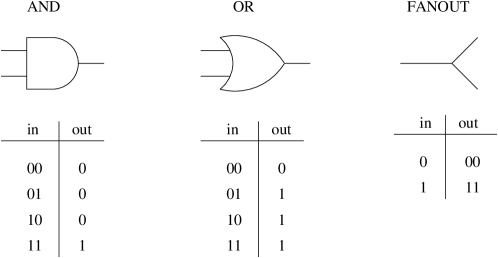
Figure 1.3: These gates are universal for classical computation. Below each gate is the corresponding “truth table” giving the dependence of output on input.

Classically, any Boolean function can be constructed using only AND, NOT, and FANOUT, as shown in figure 1.3. Thus, this set of gates are said to be universal. Similarly, the set of two-qubit quantum gates is universal in the sense that any unitary on $n$-qubits can be constructed as a product of such gates. In general, this can require exponentially many gates, much like the classical case. The proof that two-qubit gates are universal is given in detail in [137], so I will only sketch it here. The approach is to first show that the set of two level unitaries are universal. A two-level unitary is one which interacts two basis states unitarily and leaves all other states untouched, as shown below.

$$\left[\begin{array}[]{cccccccc}1&&&&&&&\\ &\ddots&&&&&&\\ &&u_{11}&&u_{12}&&&\\ &&&1&&&&\\ &&u_{21}&&u_{22}&&&\\ &&&&&1&&\\ &&&&&&\ddots&\\ &&&&&&&1\end{array}\right]$$

Given any arbitrary $2^{n}\times 2^{n}$ unitary, one can left-multiply by a sequence of two-level unitaries to eliminate off-diagonal matrix elements one by one. This process is somewhat analogous to Gaussian elimination. At the same time, one can also ensure that the remaining diagonal elements are all equal to 1. That is, for any unitary $U$ on $n$ qubits, there is some sequence of two-level unitaries $U_{m}U_{m-1}\ldots U_{2}U_{1}$ such that

$$U_{m}U_{m-1}\ldots U_{2}U_{1}U=I.$$

Thus, for any $U$, there is a product of two-level unitaries equal to $U^{-1}$, which shows that two-level unitaries are universal.

For any given pair of basis states $\left|{x}\right\rangle,\left|{y}\right\rangle$, one can construct the two level unitary that acts on them according to

$$U=\left[\begin{array}[]{cc}u_{11}&u_{12}\\ u_{21}&u_{22}\\ \end{array}\right]$$

by conjugating the single-qubit gate for $U$ with a matrix $U_{\pi}$ that permutes the basis so that $U_{\pi}\left|{x}\right\rangle$ and $U_{\pi}\left|{y}\right\rangle$ differ on a single bit. It is a simple exercise to show that $U_{\pi}$ can always be constructed by a sequence of controlled-not (CNOT) gates. CNOT is a two-qubit gate that act on two-qubits according to:

$$\left[\begin{array}[]{cccc}1&0&0&0\\ 0&1&0&0\\ 0&0&0&1\\ 0&0&1&0\end{array}\right]\begin{array}[]{c}00\\ 01\\ 10\\ 11\end{array}.$$ (1.1)

The bitstrings on the right label the four computational basis states of the two qubits. The controlled-not gets its name from the fact that a NOT gate is applied to the second bit (the target bit) only if the first bit (the control bit) is 1.

Although this gate universality result is a very nice first step, it is still not fully satisfying. The set of two-qubit gates ($4\times 4$ unitary matrices) forms a continuum. An infinite number of bits would be necessary to exactly specify particular gate. The same goes for one-qubit gates ($2\times 2$ unitary matrices). However, this is a surmountable problem. The reason is that small deviations from the desired gate will cause only small probability of error in the final measurement. This is because the deviations from the desired state caused by each gate add at most linearly, which we no show, following [137].

Suppose we wish to perform the gate $V$ followed by the gate $U$. In reality we perform imprecise versions of these, $V^{\prime}$ followed by $U^{\prime}$. We’ll quantify the error introduced by the imprecise gates by

$$E(U^{\prime}V^{\prime})\equiv\max_{\langle\psi|\psi\rangle=1}\|U^{\prime}V^{\prime}\left|{\psi}\right\rangle-UV\left|{\psi}\right\rangle\|,$$

which equals

$$=\max_{\langle\psi|\psi\rangle=1}\|(UV\left|{\psi}\right\rangle-UV^{\prime}\left|{\psi}\right\rangle)+(UV^{\prime}\left|{\psi}\right\rangle-U^{\prime}V^{\prime}\left|{\psi}\right\rangle)\|.$$

By the triangle inequality this is at most

$$\leq\max_{\langle\psi|\psi\rangle=1}\|UV\left|{\psi}\right\rangle-UV^{\prime}\left|{\psi}\right\rangle\|+\|UV^{\prime}\left|{\psi}\right\rangle-U^{\prime}V^{\prime}\left|{\psi}\right\rangle\|.$$

By unitarity, this is at most

$$\leq\max_{\langle\psi|\psi\rangle=1}\|V\left|{\psi}\right\rangle-V^{\prime}\left|{\psi}\right\rangle\|+\max_{\langle\phi|\phi\rangle=1}\|U\left|{\phi}\right\rangle-U^{\prime}\left|{\phi}\right\rangle\|$$

$$=E(V^{\prime})+E(U^{\prime}).$$

Thus

$$E(U^{\prime}V^{\prime})\leq E(V^{\prime})+E(U^{\prime}).$$ (1.2)

By equation 1.2, one sees that it is not necessary to obtain higher than polynomial accuracy in the gates in order to implement quantum circuits of polynomial size. Hence only logarithmically many bits are needed to specify a gate. This result can be improved upon in two ways. First, it turns out that it is unnecessary to have even a polynomially large set of gates. Instead, arbitrary one and two qubit gates can always be constructed with polynomial accuracy using a sequence of logarithmically many gates chosen from some finite set of universal quantum gates. This result is known as the Solovay-Kitaev theorem, which we state formally below. Universal sets of quantum gates are known with as few as two gates. Secondly, the fault tolerance threshold theorem shows (among other things) that it is in fact unnecessary to achieve higher than constant accuracy in implementing each gate. Fault tolerance thresholds are discussed in section 1.5.

The following is a formal statement of the Solovay-Kitaev theorem adapted from[116].

Theorem 1 (Solovay-Kitaev).

Suppose matrices $U_{1},\ldots,U_{r}$ generate a dense subgroup in $SU(d)$. Then, given a desired unitary $U\in SU(d)$, and a precision parameter $\delta>0$, there is an algorithm to find a product $V$ of $U_{1},\ldots,U_{r}$ and their inverses such that $\|V-U\|\leq\delta$. The length of the product and the runtime of the algorithm are both polynomial in $\log(1/\delta)$.

Combining this with the universality of two-qubit unitaries, one sees that any set of one-qubit and two-qubit gates that generates a dense subgroup of $SU(4)$ is universal for quantum computation. A convenient universal set of quantum gates is the CNOT, Hadamard, and $\pi/8$ gates. The CNOT gate we have encountered already in equation 1.1. The Hadamard gate is

$$H=\frac{1}{\sqrt{2}}\left[\begin{array}[]{cc}1&1\\ 1&-1\end{array}\right],$$

and the $\pi/8$ gate is

$$T=\left[\begin{array}[]{cc}e^{-i\pi/8}&0\\ 0&e^{i\pi/8}\end{array}\right].$$

Although two-qubit gates are universal, it does not follow that arbitrary unitaries can be constructed efficiently from two-qubit gates. In fact, even the set of $2^{n}\times 2^{n}$ permutation matrices (corresponding to reversible computations) is doubly exponentially large, whereas the set of polynomial size quantum circuits is only singly exponentially large, given any discrete set of gates. Thus, some unitaries on $n$-qubits require exponentially many gates to construct as a function of $n$.

We have now seen that using a discrete set of quantum gates we can construct arbitrary unitaries, although some $n$-qubit unitaries require exponentially many gates. This is in some sense a universality result. However, what we are really interested in is computational universality. At present it is not yet obvious that one can even efficiently perform universal classical computation with such a set of gates. However, it turns out that this is indeed possible. It would be surprising if this were not possible, since classical physics, upon which classical computaters are based, is a limiting case of quantum physics. Nevertheless showing how to specifically implement classical computation with a quantum circuit is not trivial. The essential difficulty is that the standard sets of universal classical gates include gates which lose information. For example, the AND gate takes two bits of input and produces only a single bit of output. There is no way of deducing what the input was just by reading the output. In contrast, the quantum mechanical time evolution of a closed system is unitary and therefore never loses any information.

The solution to this conundrum actually predates the field of quantum computation and goes by the name of reversible circuits. It turns out that universal classical computation can be achieved using gates that have the same number of output bits as input bits, and which furthermore never lose any information. That is, the map of inputs to outputs is injective. These are called reversible gates. The CNOT gate described in equation 1.1 is an example of a classical reversible gate which has truth table

$$\begin{array}[]{c}00\to 00\\ 01\to 01\\ 10\to 11\\ 11\to 10\end{array}.$$

By itself, CNOT is not universal. However, the Fredkin gate, or controlled SWAP is. This gate has the truth table

$$\begin{array}[]{c}000\to 000\\ 001\to 001\\ 010\to 010\\ 011\to 011\\ 100\to 100\\ 101\to 110\\ 110\to 101\\ 111\to 111\end{array}.$$

The second pair of bits are swapped only if the first bit is 1. As shown in figure 1.4, AND, NOT, and FANOUT can all be implemented using the Fredkin gate. In standard non-reversible classical circuits one normally takes FANOUT for granted, considering it to be achieved by splitting a wire. In the context of reversible computing one must be more careful. The FANOUT operation requires the use of an additional bit initialized to the 0 state to take the copied value of the bit undergoing FANOUT. In fact, each of the constructions shown in figure 1.4 require initialized work bits, known as ancilla bits. This is a generic feature of reversible computation because “garbage” bits cannot be erased and instead are simply carried to the end of the computation.

Figure 1.4: The left circuit uses a controllod-SWAP (i.e. a Fredkin gate) to achieve AND using one ancilla bit initialized to zero. The right circuit uses a Fredkin gate to achieve NOT and FANOUT using two ancilla bits initialized to zero and one. AND, NOT, and FANOUT are universal for classical computation, thus classical computation can be performed reversibly using Fredkin gates and ancilla bits.

Because AND, NOT, and FANOUT can each be constructed from a single Fredkin gate, it follows that taking classical circuits and making them reversible incurs only constant overhead. Thus, the set of problems solvable in polynomial time on uniform families of reversible circuits is exactly P. On a quantum computer, a reversible 3-qubit gate such as the Fredkin gate corresponds to an 3-qubit quantum gate which is an $8\times 8$ permutation matrix, permuting the basis states in accordance with the gate’s truth table. Hence reversible computation is efficiently achievable on quantum computers. Because of this generic construction, current research on quantum algorithms focuses on quantum algorithms which beat the best classical algorithms. Quantum algorithms matching the performance of classical algorithms can always be achieved using reversible circuits.

For the purpose of quantum computation it is often important to remove the garbage qubits accumulated at the end of a reversible computation, because these can destroy the interference needed in quantum algorithms. It is always possible to remove the garbage bits by first performing the reversible computation, then using CNOT gates to copy the result into a register of ancilla bits initialized to zero, and then reversing the computation, as illustrated in figure 1.5. The process of reversing the computation is known as uncomputation.

Figure 1.5: Garbage bits can be reset to zero. This is done by first performing the computation, then copying the output into an ancilla register, then using the inverse computation to “uncompute” the garbage bits.

The quantum circuit model is used as the standard definition of quantum computers. The class of problems solvable in polynomial time with quantum circuits is called BQP, which stands for Bounded-error Quantum Polynomial-time. The initial state given to the quantum circuit must be a computational basis state corresponding to a bitstring encoding the problem instance, plus optionally a supply of polynomially many ancilla qubits initialized to $\left|{0}\right\rangle$. The output is obtained by measuring a single qubit in the computational basis. BQP is a class of decision problems, and the measurement outcome is considered to be yes or no depending on whether the measurement yields one or zero. A decision problem belongs to BQP if there exists a uniform family of quantum circuits whose number of gates scales polynomially with the input size $n$, such that the output is correct with probability at least 2/3 for every problem instance. BQP is thus the quantum analogue of BPP.

A family of quantum circuits is considered to be uniform if the circuit for any given $n$ can be generated in $\mathrm{poly}(n)$ time by a classical computer. Allowing the family of circuits to be generated by a quantum computer does not increase the power of the model. This is a consequence of the principle of deferred measurement, as discussed in appendix E.

Because probabilities arise naturally in quantum mechanics, most studies of quantum computation focus on probabilistic computations and complexity classes. Deterministic quantum computation can certainly be defined, and some quantum algorithms succeed with probability one while still achieving a speedup over classical computation. However, restricting to deterministic quantum algorithms seems somewhat artificial. Most of the literature on quantum algorithms and complexity assumes the probabilistic setting by default, as does this thesis.

Recall that MA is the probabilistic version of NP. That is, it is the class of problems whose YES instances have probabilistically verifiable witnesses. There are two quantum analogues to MA, depending on whether the witnesses are classical or quantum. The set of decision problems whose solutions are efficiently verifiable on a quantum computer given a classical bitstring as a witness is called QCMA. The set of decision problems whose solutions are efficiently verifiable on a quantum computer given a quantum state as a witness is called QMA. Many important physical problems are now known to be QMA complete, such as computing the ground state energy of arbitrary Hamiltonians made from two-body interactions[113], and determining the consistency of a set of density matrices[124]. One can also define space bounded quantum computation. BQPSPACE is the class of problems solvable with bounded error on a quantum computer with polynomial space and unlimited time. Perhaps surprisingly, BQPSPACE = PSPACE [170]. (As an aside, NPSPACE = PSPACE [156]!)

The class of problems solvable by logarithmic depth quantum circuits is called BQNC1. This class is potentially relevant for physical implementation of quantum computers because if quantum gates can be performed in parallel, then the BQNC1 computations can be carried out in logarithmic time. This greatly reduces the time one needs to maintain the coherence of the qubits. Interestingly, an approximate quantum Fourier transform can be done using a logarithmic depth quantum circuit. As a result, factoring can be done with polynomially many uses of logarithmic depth quantum circuits, followed by a polynomial amount of classical postprocessing[48].

As mentioned previously, it is easy to see that problems solvable in classical space $f(n)$ are solvable in classical time $2^{f(n)}$ ecause there are only $2^{f(n)}$ states that the computer can be in. Thus, after $2^{f(n)}$ steps the computer must reenter a previously used state and repeat itself. Quantum mechanically the situation is different. For any fixed $\epsilon\ll 1$, in a Hilbert space of dimension $d$ one can fit exponentially many nonoverlapping patches of size $\epsilon$ as a function of $d$. (We could define a patch of size $\epsilon$ centered at $\left|{\psi}\right\rangle$ as $\{\left|{\phi}\right\rangle:\|\left|{\phi}\right\rangle-\left|{\psi}\right\rangle\|<\epsilon\}$.) Thus there are doubly exponentially many reasonably distinct states of $n$ qubits. Hence there is not an analogous argument to show that problems solvable in quantum space $f(n)$ are solvable in quantum time $\mathrm{exp}(f(n))$. Nevertheless, this statement is true. It can be proven using the previously described universality construction based on two level unitaries. Working through the construction in detail one finds that any $2^{n}\times 2^{n}$ unitary can be constructed from $O(2^{2n})$ two level unitaries, and any 2-level unitary on the Hilbert space of $n$ qubits can be achieved using $O(n^{2})$ CNOT gates plus one arbitrary single-qubit gate. Thus no computation on $n$-qubits can require more than $O(2^{2n}n^{2})$ gates. (However, finding the appropriate gate sequence may be difficult.)

1.3 Quantum Algorithms

1.3.1 Introduction

By now it is well-known that quantum computers can solve certain problems much faster than the best known classical algorithms. The most famous example is that quantum computers can factor $n$-bit numbers in time polynomial in $n$[160], whereas no known classical algorithm can do this. The quantum algorithm which achieves this is known as Shor’s factoring algorithm. As discussed in section 1.2, a quantum algorithm can be defined as a uniform family of quantum circuits, and the running time is the number of gates as a function of number of bits of input.

Quantum algorithms can be categorized into two types based on the method by which the problem instance is given to the quantum computer. The most most obvious and fundamental way to provide the input is as a bitstring. This is how the input is provided to the factoring algorithm. The second way of providing the input to a quantum algorithm is through an oracle. The oracular setting is very much analogous to the classical oracular setting, with the additional restriction that the oracle must be unitary. Any classical oracle can be made unitary by the general technique of reversible computation, as shown in figure 1.6.

Figure 1.6: Quantum oracles must be unitary. One can always achieve this by using separate input and output registers. The input register is left unchanged and the output is added into the output register bitwise modulo 2. If the input register $y$ is initialized $0000\ldots$, than after applying the oracle it will contain $f(x)$.

The second most famous quantum algorithm is oracular. The oracle implements the function $f:\{0,1,\ldots,N\}\to\{0,1\}$ defined by

$$f(x)=\left\{\begin{array}[]{ll}1&\textrm{if $x=w$}\\ 0&\textrm{otherwise}\end{array}\right.$$

The task is to find the “winner” $w$. Classically, the only way to do this with guaranteed success is to query all $N$ values of $x$. Even on average, one needs to query $N/2$ values. On a quantum computer this can be achieved using $O(\sqrt{N})$ queries[86]. The algorithm which achieves this is known as Grover’s searching algorithm. The queries made to the oracle are superpositions of multiple inputs. Quantum computers cannot solve this problem using fewer than $\Omega(\sqrt{N})$ queries[23]. Brute-force searching is a common subroutine in classical algorithms. Thus, many classical algorithms can be sped up by using Grover search as a subroutine. Furthermore, quantum algorithms achieve quadratic speedups for searching in the presence of more than one winner[31], evaluating sum of an arbitrary function[31, 32, 131], finding the global minimum of arbitrary function[62, 135], and approximating definite integrals[139]. These algorithms are based on Grover’s search algorithm.

From a complexity point of view, a quantum algorithm provides an upper bound on the quantum complexity of a given problem. It is also interesting to look for lower bounds on the quantum complexity problems, or in other words upper limits on the power of quantum computers. The techniques for doing so are very different in the oracular versus nonoracular settings.

In the oracular setting, several powerful methods are known for proving lower bounds on the quantum query complexity of problems[11, 21]. The $\Omega(\sqrt{N})$ lower bound for searching is one example of this. For some oracular problems it is proven that quantum computers do not offer any speedup over classical computers beyond a constant factor. For example, suppose we are given an oracle computing an arbitrary function of the form $f:\{0,1,\ldots,N\}\to\{0,1\}$, and we wish to compute the parity

$$\bigoplus_{x=1}^{N}f(x).$$

Both quantum and classical computers need $\Omega(N)$ queries to achive this[67].

In the non-oracular setting there are essentially no known techniques for proving lower bounds on quantum (or classical) complexity. One can see however that quantum computers cannot achieve superexponential speedups over classical computers because they can be classically simulated with exponential overhead. Extending this reasoning, it is clear that one could show by diagonalization[141] that for any polynomial $p(n)$ there exist problems in EXP which cannot be solved on a quantum computer in time less than $p(n)$. A different type of upper bound on the power of quantum computers is that $\textrm{BQP}\in P^{\#P}$, as shown in[24].

Arguably the most important class of known quantum algorithms from a practical point of view are those for quantum simulation. The problem of simulating quantum systems has great economic and scientific significance. Many problems, such as the design of new drugs and materials, and understanding condensed matter systems such as high temperature superconductors, would likely be much easier if quantum many-body systems could be efficiently simulated. It seems that this cannot be done on classical computers because the dimension of the Hilbert space grows exponentially with the number of degrees of freedom. Thus, even writing down the wavefunction would require exponential resources.

In contrast to classical computers, it is generally believed that standard quantum computers can efficiently simulate all nonrelativistic quantum systems. That is, the number of gates and number of qubits needed to simulate a system of $n$ particles for time $t$ should scale polynomially in $n$ and $t$. The essential reason for this is that Hamiltonians arising in nature generally consist of few-body interactions. Few-body interactions can be simulated using few-body quantum gates via the Trotter formula. The exact form of the few-body interactions is irrelevant due to gate universality. Furthermore, even if a Hamiltonian is not a sum of few-body terms, it can still be efficiently simulated provided that each row of the matrix has at most polynomially many nonzero entries and these entries can be computed efficiently. Methods for quantum simulation are described in [72, 43, 179, 172, 7, 3, 25, 109, 123]. If a physical system were discovered that could not be simulated in polynomial time by a quantum computer, and that systems could be reliably controlled, then it could presumably be used to construct a computer more powerful standard quantum computers. Currently, it is not fully known whether relativistic quantum field theory can be efficiently simulated by quantum computers. In fact, the task of formulating a well-defined mathematical theory of computation based on quantum field theory appears to be difficult.

Not all quantities that arise in the study of physics are easily computable using quantum computers. For example, finding the ground energy of an arbitrary local Hamiltonian is QMA-hard[113], and evaluating the partition function of the classical Potts model is #P-hard. Therefore it is unlikely that these problems can be solved in general on a quantum computer in polynomial time. It is perhaps not surprising that some partition functions cannot be efficiently evaluated, because partition functions are not directly measurable by physical means, and thus not computable by the simulation of a physical process. In contrast, information about the eigenenergies of physical systems can be measured by spectroscopy. The problem is, for some systems, the time needed to cool them into the ground state may be extremely long. Correspondingly, on a quantum computer, the energy of a given eigenstate can be efficiently determined to polynomial precision by the method of phase estimation (see appendix C), but there may be no efficient method to prepare the ground state.

Several other quantum algorithms are known. A list of known quantum algorithms is given below. I have attempted to be comprehensive, although there are probably a few oversights. By known results regarding reversible computation, any classical algorithm can be implemented on a quantum computer with only constant overhead. Thus, I only list quantum algorithms achieving a speedup over the fastest known classical algorithm. Furthermore, any quantum circuit solves the problem of computing its own output. Thus to keep the list meaningful, I include only quantum algorithms achieving a speedup for a problem that could have been stated prior to the concept of quantum computation (although not all of these problems necessarily were). Most quantum algorithms in the literature meet this criterion.

1.3.2 Algebraic and Number Theoretic Problems

Algorithm: Factoring
Type: Non-oracular
Speedup: Superpolynomial
Description: Given an $n$-bit integer, find the prime factorization. The quantum algorithm of Peter Shor solves this in $\mathrm{poly}(n)$ time[160]. The fastest known classical algorithm requires time superpolynomial in $n$. This algorithm breaks the RSA cryptosystem. At the core of this algorithm is order finding, which can be reduced to the Abelian hidden subgroup problem.

Algorithm: Discrete-log
Type: Non-oracular
Speedup: Superpolynomial
Description: We are given three $n$-bit numbers $a$, $b$, and $N$, with the promise that $b=a^{s}\mod N$ for some $s$. The task is to find $s$. As shown by Shor[160], this can be achieved on a quantum computer in $\mathrm{poly}(n)$ time. The fastest known classical algorithm requires time superpolynomial in $n$. See also Abelian hidden subgroup.

Algorithm: Pell’s Equation
Type: Non-oracular
Speedup: Superpolynomial
Description: Given a positive nonsquare integer $d$, Pell’s equation is $x^{2}-dy^{2}=1$. For any such $d$ there are infinitely many pairs of integers $(x,y)$ solving this equation. Let $(x_{1},y_{1})$ be the pair that minimizes $x+y\sqrt{d}$. If $d$ is an $n$-bit integer (i.e. $0\leq d<2^{n}$), then $(x_{1},y_{1})$ may in general require exponentially many bits to write down. Thus it is in general impossible to find $(x_{1},y_{1})$ in polynmial time. Let $R=\log(x_{1}+y_{1}\sqrt{d})$. $\lfloor R\rceil$ uniquely identifies $(x_{1},y_{1})$. As shown by Hallgren[88], given a $n$-bit number $d$, a quantum computer can find $\lfloor R\rceil$ in $\mathrm{poly}(n)$ time. No polynomial time classical algorithm for this problem is known. Factoring reduces to this problem. This algorithm breaks the Buchman-Williams cryptosystem. See also Abelian hidden subgroup.

Algorithm: Principal Ideal
Type: Non-oracular
Speedup: Superpolynomial
Description: We are given an $n$-bit integer $d$ and an invertible ideal $I$ of the ring $\mathbb{Z}[\sqrt{d}]$. $I$ is a principal ideal if there exists $\alpha\in\mathbb{Q}(\sqrt{d})$ such that $I=\alpha\mathbb{Z}[\sqrt{d}]$. $\alpha$ may be exponentially large in $d$. Therefore $\alpha$ cannot in general even be written down in polynomial time. However, $\lfloor\log\alpha\rceil$ uniquely identifies $\alpha$. The task is to determine whether $I$ is principal and if so find $\lfloor\log\alpha\rceil$. As shown by Hallgren, this can be done in polynomial time on a quantum computer[88]. Factoring reduces to solving Pell’s equation, which reduces to the principal ideal problem. Thus the principal ideal problem is at least as hard as factoring and therefore is probably not in P. See also Abelian hidden subgroup.

Algorithm: Unit Group
Type: Non-oracular
Speedup: Superpolynomial
Description: The number field $\mathbb{Q}(\theta)$ is said to be of degree $d$ if the lowest degree polynomial of which $\theta$ is a root has degree $d$. The set $\mathcal{O}$ of elements of $\mathbb{Q}(\theta)$ which are roots of monic polynomials in $\mathbb{Z}[x]$ forms a ring, called the ring of integers of $\mathbb{Q}(\theta)$. The set of units (invertible elements) of the ring $\mathcal{O}$ form a group denoted $\mathcal{O}^{*}$. As shown by Hallgren [89], for any $\mathbb{Q}(\theta)$ of fixed degree, a quantum computer can find in polynomial time a set of generators for $\mathcal{O}^{*}$, given a description of $\theta$. No polynomial time classical algorithm for this problem is known. See also Abelian hidden subgroup.

Algorithm: Class Group
Type: Non-oracular
Speedup: Superpolynomial
Description: The number field $\mathbb{Q}(\theta)$ is said to be of degree $d$ if the lowest degree polynomial of which $\theta$ is a root has degree $d$. The set $\mathcal{O}$ of elements of $\mathbb{Q}(\theta)$ which are roots of monic polynomials in $\mathbb{Z}[x]$ forms a ring, called the ring of integers of $\mathbb{Q}(\theta)$. For a ring, the ideals modulo the prime ideals form a group called the class group. As shown by Hallgren[89], a quantum computer can find in polynomial time a set of generators for the class group of the ring of integers of any constant degree number field, given a description of $\theta$. No polynomial time classical algorithm for this problem is known. See also Abelian hidden subgroup.

Algorithm: Hidden Shift
Type: Oracular
Speedup: Superpolynomial
Description: We are given oracle access to some function $f(x)$ on a domain of size $N$. We know that $f(x)=g(x+s)$ where $g$ is a known function and $s$ is an unknown shift. The hidden shift problem is to find $s$. By reduction from Grover’s problem it is clear that at least $\sqrt{N}$ queries are necessary to solve hidden shift in general. However, certain special cases of the hidden shift problem are solvable on quantum computers using $O(1)$ queries. In particular, van Dam et al. showed that this can be done if $f$ is a multiplicative character of a finite ring or field[167]. The previously discovered shifted Legendre symbol algorithm[166, 164] is subsumed as a special case of this, because the Legendre symbol $\left(\frac{x}{p}\right)$ is a multiplicative character of $\mathbb{F}_{p}$. No classical algorithm running in time $O(\mathrm{polylog}(N))$ is known for these problems. Furthermore, the quantum algorithm for the shifted Legendre symbol problem breaks certain classical cryptosystems[167].

Algorithm: Gauss Sums
Type: Non-oracular
Speedup: Superpolynomial
Description: Let $\mathbb{F}_{q}$ be a finite field. The elements other than zero of $\mathbb{F}_{q}$ form a group $\mathbb{F}_{q}^{\times}$ under multiplication, and the elements of $\mathbb{F}_{q}$ form an (Abelian but not necessarily cyclic) group $\mathbb{F}_{q}^{+}$ under addition. We can choose some representation $\rho^{\times}$ of $\mathbb{F}_{q}^{\times}$ and some representation $\rho^{+}$ of $\mathbb{F}_{q}^{+}$. Let $\chi^{\times}$ and $\chi^{+}$ be the characters of these representations. The Gauss sum corresponding to $\rho^{\times}$ and $\rho^{+}$ is the inner product of these characters: $\sum_{x\neq 0\in\mathbb{F}_{q}}\chi^{+}(x)\chi^{\times}(x)$. As shown by van Dam and Seroussi[168], Gauss sums can be estimated to polynomial precision on a quantum computer in polynomial time. Although a finite ring does not form a group under multiplication, its set of units does. Choosing a representation for the additive group of the ring, and choosing a representation for the multiplicative group of its units, one can obtain a Gauss sum over the units of a finite ring. These can also be estimated to polynomial precision on a quantum computer in polynomial time[168]. No polynomial time classical algorithm for estimating Gauss sums is known. Furthermore, discrete log reduces to Gauss sum estimation.

Algorithm: Abelian Hidden Subgroup
Type: Oracular
Speedup: Exponential
Description: Let $G$ be a finitely generated Abelian group, and let $H$ be some subgroup of $G$ such that $G/H$ is finite. Let $f$ be a function on $G$ such that for any $g_{1},g_{2}\in G$, $f(g_{1})=f(g_{2})$ if and only if $g_{1}$ and $g_{2}$ are in the same coset of $H$. The task is to find $H$ (i.e. find a set of generators for $H$) by making queries to $f$. This is solvable on a quantum computer using $O(\log|G|)$ queries, whereas classically $\Omega(|G|)$ are required. This algorithm was first formulated in full generality by Boneh and Lipton in [30]. However, proper attribution of this algorithm is difficult because, as described in chapter 5 of [137], it subsumes many historically important quantum algorithms as special cases, including Simon’s algorithm, which was the inspiration for Shor’s period finding algorithm, which forms the core of his factoring and discrete-log algorithms. The Abelian hidden subgroup algorithm is also at the core of the Pell’s equation, principal ideal, unit group, and class group algorithms. In certain instances, the Abelian hidden subgroup problem can be solved using a single query rather than $\log(|G|)$, see [55].

Algorithm: Non-Abelian Hidden Subgroup
Type: Oracular
Speedup: Exponential
Description: Let $G$ be a finitely generated group, and let $H$ be some subgroup of $G$ that has finitely many left cosets. Let $f$ be a function on $G$ such that for any $g_{1},g_{2}\in G$, $f(g_{1})=f(g_{2})$ if and only if $g_{1}$ and $g_{2}$ are in the same left coset of $H$. The task is to find $H$ (i.e. find a set of generators for $H$) by making queries to $f$. This is solvable on a quantum computer using $O(\log(|G|)$ queries, whereas classically $\Omega(|G|)$ are required[65, 90]. However, this does not qualify as an efficient quantum algorithm because in general, it may take exponential time to process the quantum states obtained from these queries. Efficient quantum algorithms for the hidden subgroup problem are known for certain specific non-Abelian groups[150, 98, 130, 96, 17, 38, 99, 127, 100, 75, 77, 46]. A slightly outdated survey is given in [125]. Of particular interest are the symmetric group and the dihedral group. A solution for the symmetric group would solve graph isomorphism. A solution for the dihedral group would solve certain lattice problems[147]. Despite much effort, no polynomial-time solution for these groups is known. However, Kuperburg[120] found a time $O(2^{C\sqrt{\log N}})$ algorithm for finding a hidden subgroup of the dihedral group $D_{N}$. Regev subsequently improved this algorithm so that it uses not only subexponential time but also polynomial space[148].

1.3.3 Oracular Problems

Algorithm: Searching
Type: Oracular
Speedup: Polynomial
Description: We are given an oracle with $N$ allowed inputs. For one input $w$ (“the winner”) the corresponding output is 1, and for all other inputs the corresponding output is 0. The task is to find $w$. On a classical computer this requires $\Omega(N)$ queries. The quantum algorithm of Lov Grover achieves this using $O(\sqrt{N})$ queries[86].This has algorithm has subsequently been generalized to search in the presence of multiple “winners”[31], evaluate the sum of an arbitrary function[31, 32, 131], find the global minimum of an arbitrary function[62, 135], and approximate definite integrals[139]. The generalization of Grover’s algorithm known as amplitude estimation[33] is now an important primitive in quantum algorithms. Amplitude estimation forms the core of most known quantum algorithms related to collision finding and graph properties.

Algorithm: Bernstein-Vazirani
Type: Oracular
Speedup: Polynomial
Description: We are given an oracle whose input is $n$ bits and whose output is one bit. Given input $x\in\{0,1\}^{n}$, the output is $x\odot h$, where $h$ is the “hidden” string of $n$ bits, and $\odot$ denotes the bitwise inner product modulo 2. The task is to find $h$. On a classical computer this requires $n$ queries. As shown by Bernstein and Vazirani[24], this can be achieved on a quantum computer using a single query. Furthermore, one can construct a recursive version of this problem, called recursive Fourier sampling, such that quantum computers require exponentially fewer queries than classical computers[24].

Algorithm: Deutsch-Josza
Type: Oracular
Speedup: Polynomial
Description: We are given an oracle whose input is $n$ bits and whose output is one bit. We are promised that out of the $2^{n}$ possible inputs, either all of them, none of them, or half of them yield output 1. The task is to distinguish the balanced case (half of all inputs yield output 1) from the constant case (all or none of the inputs yield output 1). It was shown by Deutsch[57] that for $n=1$, this can be solved on a quantum computer using one query, whereas any deterministic classical algorithm requires two. This was historically the first well-defined quantum algorithm achieving a speedup over classical computation. The generalization to arbitrary $n$ was developed by Deutsch and Josza in [58]. Although probabilistically easy to solve with $O(1)$ queries, the Deutsch-Josza problem has exponential worst case deterministic query complexity classically.

Algorithm: NAND Tree
Type: Oracular
Speedup: Polynomial
Description: A NAND gate takes two bits of input and produces one bit of output. By connecting together NAND gates, one can thus form a binary tree of depth $n$ which has $2^{n}$ bits of input and produces one bit of output. The NAND tree problem is to evaluate the output of such a tree by making queries to an oracle which stores the values of the $2^{n}$ bits and provides any specified one of them upon request. Farhi et al. used a continuous time quantum walk model to show that a quantum computer can solve this problem using $O(2^{0.5n})$ time whereas a classical computer requires $\Omega(2^{0.753n})$ time[66]. It was soon shown that this result carries over into the conventional model of circuits and queries[45]. The algorithm was subsequently generalized for NAND trees of varying fanin and noniform depth[13], and to trees involving larger gate sets[149], and MIN-MAX trees [47].

Algorithm: Gradients
Type: Oracular
Speedup: Polynomial
Description: We are given a oracle for computing some smooth function $f:\mathbb{R}^{d}\to\mathbb{R}$. The inputs and outputs to $f$ are given to the oracle with finitely many bits of precision. The task is to estimate $\nabla f$ at some specified point $\mathbf{x}_{0}\in\mathbb{R}^{d}$. As I showed in [107], a quantum computer can achieve this using one query, whereas a classical computer needs at least $d+1$ queries. In [36], Bulger suggested potential applications for optimization problems[36]. As shown in appendix D, a quantum computer can use the gradient algorithm to find the minimum of a quadratic form in $d$ dimensions using $O(d)$ queries, whereas, as shown in [177], a classical computer needs at least $\Omega(d^{2})$ queries.

Algorithm: Ordered Search
Type: Oracular
Speedup: Constant
Description: We are given oracle access to a list of $N$ numbers in order from least to greatest. Given a number $x$, the task is to find out where in the list it would fit. Classically, the best possible algorithm is binary search which takes $\log_{2}N$ queries. Farhi et al. showed that a quantum computer can achieve this using $0.53\log(N)$ queries[68]. Currently, the best known deterministic quantum algorithm for this problem uses $0.433\log_{2}N$ queries. A lower bound of $\frac{1}{\pi}\log_{2}N$ quantum queries has been proven for this problem[42]. In [22], a randomized quantum algorithm is given whose expected query complexity is less than $\frac{1}{3}\log_{2}N$.

Algorithm: Graph Properties
Type: Oracular
Speedup: Polynomial
Description: A common way to specify a graph is by an oracle, which given a pair of vertices, reveals whether they are connected by an edge. This is called the adjacency matrix model. It generalizes straightforwardly for weighted and directed graphs. Building on previous work [62, 94, 63], Dürr et al. [61] show that the quantum query complexity of finding a minimum spanning tree of weighted graphs, and deciding connectivity for directed and undirected graphs have $\Theta(n^{3/2})$ quantum query complexity, and that finding lowest weight paths has $O(n^{3/2}\log^{2}n)$ quantum query complexity. Berzina et al. [26] show that deciding whether a graph is bipartite can be achieved using $O(n^{3/2})$ quantum queries. All of these problems are thought to have $\Omega(n^{2})$ classical query complexity. For many of these problems, the quantum complexity is also known for the case where the oracle provides an array of neighbors rather than entries of the adjacency matric[61]. See also triangle finding.

Algorithm: Welded Tree
Type: Oracular
Speedup: Exponential
Description: Some computational problems can be phrased in terms of the query complexity of finding one’s way through a maze. That is, there is some graph $G$ to which one is given oracle access. When queried with the label of a given node, the oracle returns a list of the labels of all adjacent nodes. The task is, starting from some source node (i.e. its label), to find the label of a certain marked destination node. As shown by Childs et al.[44], quantum computers can exponentially outperform classical computers at this task for at least some graphs. Specifically, consider the graph obtained by joining together two depth-$n$ binary trees by a random “weld” such that all nodes but the two roots have degree three. Starting from one root, a quantum computer can find the other root using $\mathrm{poly}(n)$ queries, whereas this is provably impossible using classical queries.

Algorithm: Collision Finding
Type: Oracular
Speedup: Polynomial
Description: Suppose we are given oracle access to a two to one function $f$ on a domain of size $N$. The collision problem is to find a pair $x,y\in\{1,2,\ldots,N\}$ such that $f(x)=f(y)$. The classical randomized query complexity of this problem is $\Theta(\sqrt{N})$, whereas, as shown by Brassard et al., a quantum computer can achieve this using $O(N^{1/3})$ queries[34]. Buhrman et al. subsequently showed that a quantum computer can also find a collision in an arbitrary function on domain of size $N$, provided that one exists, using $O(N^{3/4}\log N)$ queries[37], whereas the classical query complexity is $\Theta(N\log N)$. The decision version of collision finding is called element distinctness, and also has $\Theta(N\log N)$ classical query complexity. Ambainis subsequently improved upon[34], achieving a quantum query complexity of $O(N^{2/3})$ for element distinctness, which is optimal, and extending to the case of $k$-fold collisions[12]. Given two functions $f$ and $g$, each on a domain of size $N$, a claw is a pair $x,y$ such that $f(x)=g(y)$. A quantum computer can find claws using $O(N^{3/4}\log N)$ queries[37].

Algorithm: Triangle Finding
Type: Oracular
Speedup: Polynomial
Description: Suppose we are given oracle access to a graph. When queried with a pair of nodes, the oracle reveals whether an edge connects them. The task is to find a triangle (i.e. a clique of size three) if one exists. As shown by Buhrman et al. [37], a quantum computer can accomplish this using $O(N^{3/2})$ queries, whereas it is conjectured that classically one must query all $\binom{n}{2}$ edges. Magniez et al. subsequently improved on this, finding a triangle with $O(N^{13/10})$ quantum queries[126].

Algorithm: Matrix Commutativity
Type: Oracular
Speedup: Polynomial
Description: We are given oracle access to $k$ matrices, each of which are $n\times n$. Given integers $i,j\in\{1,2,\ldots,n\}$, and $x\in\{1,2,\ldots,k\}$ the oracle returns the $ij$ matrix element of the $x^{\mathrm{th}}$ matrix. The task is to decide whether all of these $k$ matrices commute. As shown by Itakura[97], this can be achieved on a quantum computer using $O(k^{4/5}n^{9/5})$ queries, whereas classically this requires $O(kn^{2})$ queries.

Algorithm: Hidden Nonlinear Structures
Type: Oracular
Speedup: Exponential
Description: Any Abelian groups $G$ can be visualized as a lattice. A subgroup $H$ of $G$ is a sublattice, and the cosets of $H$ are all the shifts of that sublattice. The Abelian hidden subgroup problem is normally solved by obtaining superposition over a random coset of the Hidden subgroup, and then taking the Fourier transform so as to sample from the dual lattice. Rather than generalizing to non-Abelian groups (see non-Abelian hidden subgroup), one can instead generalize to the problem of identifying hidden subsets other than lattices. As shown by Childs et al.[39] this problem is efficiently solvable on quantum computers for certain subsets defined by polynomials, such as spheres. Decker et al. showed how to efficiently solve some related problems in[56].

Algorithm: Order of Blackbox Group
Type: Oracular
Speedup: Exponential
Description: Suppose a finite group $G$ is given oracularly in the following way. To every element in $G$, one assigns a corresponding label. Given an ordered pair of labels of group elements, the oracle returns the label of their product. The task is to find the order of the group, given the labels of a set of generators. Classically, this problem cannot be solved using $\mathrm{polylog}(|G|)$ queries even if $G$ is Abelian. For Abelian groups, quantum computers can solve this problem using $\mathrm{polylog}(|G|)$ queries by reducing it to the Abelian hidden subgroup problem, as shown by Mosca[132]. Furthermore, as shown by Watrous[169], this problem can be solved in $\mathrm{polylog}(|G|)$ queries for any solvable group.

1.3.4 Approximation and BQP-complete Problems

Algorithm: Quantum Simulation
Type: Non-oracular
Speedup: Exponential
Description: It is believed that for any physically realistic Hamiltonian $H$ on $n$ degrees of freedom, the corresponding time evolution operator $e^{-iHt}$ can be implemented using $\mathrm{poly}(n,t)$ gates. Unless BPP=BQP, this problem is not solvable in general on a classical computer in polynomial time. Many techniques for quantum simulation have been developed for different applications[43, 179, 172, 7, 3, 25, 109, 123]. The exponential complexity of classically simulating quantum systems led Feynman to first propose that quantum computers might outperform classical computers on certain tasks[72].

Algorithm: Jones Polynomial
Type: Non-oracular
Speedup: Exponential
Description: As shown by Freedman[74, 73], et al., finding a certain additive approximation to the Jones polynomial of the plat closure of a braid at $e^{i2\pi/5}$ is a BQP-complete problem. This result was reformulated and extended to $e^{i2\pi/k}$ for arbitrary $k$ by Aharonov et al.[6, 4]. Wocjan and Yard further generalized this, obtaining a quantum algorithm to estimate the HOMFLY polynomial[174], of which the Jones polynomial is a special case. Aharonov et al. subsequently showed that quantum computers can in polynomial time estimate a certain additive approximation to the even more general Tutte polynomial for planar graphs[5]. The hardness of the additive approximation obtained in [5] is not yet fully understood. As discussed in chapter 3 of this thesis, the problem of finding a certain additive approximation to the Jones polynomial of the trace closure of a braid at $e^{i2\pi/5}$ is DQC1-complete.

Algorithm: Zeta Functions
Type: Non-oracular
Speedup: Superpolynomial
Description: As shown by Kedlaya[112], quantum computers can determine the zeta function of a genus $g$ curve over a finite field $\mathbb{F}_{q}$ in time polynomial in $g$ and $\log q$. No polynomial time classical algorithm for this problem is known. More speculatively, van Dam has conjectured that due to a connection between the zeros of zeta functions and the eigenvalues of certain quantum operators, quantum computers might be able to efficiently approximate the number of solutions to equations over finite fields[165]. Some evidence supporting this conjecture is given in [165].

Algorithm: Weight Enumerators
Type: Non-oracular
Speedup: Exponential
Description: Let $C$ a code on $n$ bits, i.e. a subset of $\mathbb{Z}_{2}^{n}$. The weight enumerator of $C$ is $S_{C}(x,y)=\sum_{c\in C}x^{|c|}y^{n-|c|}$, where $|c|$ denotes the Hamming weight of $c$. Weight enumerators have many uses in the study of classical codes. If $C$ is a linear code, it can be defined by $C=\{c:Ac=0\}$ where $A$ is a matrix over $\mathbb{Z}_{2}$. In this case $S_{C}(x,y)=\sum_{c:Ac=0}x^{|c|}y^{n-|c|}$. Quadratically signed weight enumerators (QWGTs) are a generalization of this: $S(A,B,x,y)=\sum_{c:Ac=0}(-1)^{c^{T}Bc}x^{|c|}y^{n-|c|}$. Now consider the following special case. Let $A$ be an $n\times n$ matrix over $\mathbb{Z}_{2}$ such that $\mathrm{diag}(A)=I$. Let $\mathrm{lwtr}(A)$ be the lower triangular matrix resulting from setting all entries above the diagonal in $A$ to zero. Let $l,k$ be positive integers. Given the promise that $|S(A,\mathrm{lwtr}(A),k,l)|\geq\frac{1}{2}(k^{2}+l^{2})^{n/2}$, the problem of determining the sign of $S(A,\mathrm{lwtr}(A),k,l)$ is BQP-complete, as shown by Knill and Laflamme in [119]. The evaluation of QWGTs is also closely related to the evaluation of Ising and Potts model partition functions[122, 78, 79, 80].

Algorithm: Simulated Annealing
Type: Non-oracular
Speedup: Polynomial
Description: In simulated annealing, one has a series of Markov chains defined by stochastic matrices $M_{1},M_{2},\ldots,M_{n}$. These are slowly varying in the sense that their limiting distributions $\pi_{1},\pi_{2},\ldots,\pi_{n}$ satisfy $|\pi_{t+1}-\pi_{t}|<\epsilon$ for some small $\epsilon$. These distributions can often be though of as thermal distributions at successively lower temperatures. If $\pi_{1}$ can be easily prepared then by applying this series of Markov chains one can sample from $\pi_{n}$. Typically, one wishes for $\pi_{n}$ to be a distribution over good solutions to some optimization problem. Let $\delta_{i}$ be the gap between the largest and second largest eigenvalues of $M_{i}$. Let $\delta=\min_{i}\delta_{i}$. The run time of this classical algorithm is proportional to $1/\delta$. Building upon results of Szegedy[162], Somma et al. have shown[161] that quantum computers can sample from $\pi_{n}$ with a runtime proportional to $1/\sqrt{\delta}$.

Algorithm: String Rewriting
Type: Non-oracular
Speedup: Exponential
Description: String rewriting is a fairly general model of computation. String rewriting systems (sometimes called grammars) are specified by a list of rules by which certain substrings are allowed to be replaced by certain other substrings. For example, context free grammars, are equivalent to the pushdown automata. In [103], Janzing and Wocjan showed that a certain string rewriting problem is PromiseBQP-complete. Thus quantum computers can solve it in polynomial time, but classical computers probably cannot. Given three strings $s$, $t$, and $t^{\prime}$, and a set of string rewriting rules satisfying certain promises, the problem is to find a certain approximation to the difference between the number of ways of obtaining $t$ from $s$ and the number of ways of obtaining $t^{\prime}$ from $s$. Similarly, certain problems of approximating the difference in number of paths between pairs of vertices in a graph, and difference in transition probabilities between pairs of states in a random walk are also BQP-complete[102].

Algorithm: Matrix Powers
Type: Non-oracular
Speedup: Exponential
Description: Quantum computers have an exponential advantage in approximating matrix elements of powers of exponentially large sparse matrices. Suppose we are have an $N\times N$ symmetric matrix $A$ such that there are at most $\mathrm{polylog}(N)$ nonzero entries in each row, and given a row index, the set of nonzero entries can be efficiently computed. The task is, for any $1<i<N$, and any $m$ polylogarithmic in $N$, to approximate $(A^{m})_{ii}$, the $i^{\mathrm{th}}$ diagonal matrix element of $A^{m}$. The approximation is additive to within $b^{m}\epsilon$, where $b$ is a given upper bound on $\|A\|$ and $\epsilon$ is of order $1/\mathrm{polylog}(N)$. As shown by Janzing and Wocjan, this problem is PromiseBQP-complete, as is the corresponding problem for off-diagonal matrix elements[104]. Thus, quantum computers can solve it in polynomial time, but classical computers probably cannot.

Algorithm: Verifying Matrix Products
Type: Non-oracular
Speedup: Polynomial
Description: Given three $n\times n$ matrices, $A$, $B$, and $C$, the matrix product verification problem is to decide whether $AB=C$. Classically, the best known algorithm achieves this in time $O(n^{2})$, whereas the best known classical algorithm for matrix multiplication runs in time $O(n^{2.376})$. Ambainis et al. discovered a quantum algorithm for this problem with runtime $O(n^{7/4})$ [10]. Subsequently, Buhrman and Špalek improved upon this, obtaining a quantum algorithm for this problem with runtime $O(n^{5/3})$ [35]. This latter algorithm is based on results regarding quantum walks that were proven in[162].

1.3.5 Commentary

As noted above, some of these algorithms break existing cryptosystems. I mention this not because I care about breaking cryptosystems, but because public key cryptosystems serve as a useful indicator of the general consensus regarding the computational difficulty of certain mathematical problems. For each known public key cryptosystem, the security proof rests on an assumption that a certain mathematical problem cannot be solved in polynomial time. As discussed in section 1.1, nobody knows how to prove that these problems cannot be solved in polynomial time. However, some of these problems, such as factoring, have resisted many years of attempts at polynomial time solution. Thus, many people consider it to be a safe assumption that factoring is hard. People and corporations also effectively wager money on this, as nearly all monetary transactions on the internet are encoded using the RSA cryptosystem, which is based on the assumption that factoring is hard to solve classically.

Many of the problems solved by these quantum algorithms may seem somewhat esoteric. Upon hearing that quantum computers can approximate Tutte polynomials or solve Pell’s equation, one may ask “Why should I care?”. One answer to this is that mathematical algorithms sometimes have applications which are not discovered until long after the algorithm itself. A deeper answer is that complexity theory has shown that the ability to solve hard computational problems is to some degree a fungible resource. That is, many hard problems reduce to one another with polynomial overhead. By finding a polynomial time solution for one hard problem, one obtains polynomial time solutions for a class of problems that can appear unrelated. An interesting example of this is the LLL algorithm, for the apparently esoteric problem of finding a basis of short vectors for a lattice. This has subsequently found application in cryptography, error correction, and finding integer relations between numbers. LLL and subsequent variants for integer relation finding have even found use in computer assisted mathematics. Their achievements include, among other things, the discovery of a new formula for the digits of $\pi$ such that any digit of $\pi$ can be calculated using a constant amount of computation without having to calculate the preceeding digits[18]!

In light of such history, and in light of known properties of computational complexity, it makes sense to search for quantum algorithms that provide polynomial speedups for problems of direct practical relevance, and to try to find exponential speedups for any problem.

1.4 What makes quantum computers powerful?

The quantum algorithms described in section 1.3 establish rigorously that quantum computers can solve some problems using far fewer queries than classical computers, and establish convincingly that quantum computers can solve certain problems using far fewer computational steps than classical computers. It is natural to ask what aspect of quantum mechanics gives quantum computers their extra computational power. At first glance this appears to be a vague and ill-posed question. However, we can approach this question in a concrete way by taking away different aspects of quantum mechanics one at a time, and seeing whether the resulting models of computation retain the power of quantum computers.

One necessary ingredient for the power of quantum computing is the exponentially high-dimensional Hilbert space. If we take this away, then the resulting model of computation can be simulated in polynomial time by a classical compute. To simulate the action of each gate, one would need only to multiply the state vector by a unitary matrix of polynomial dimension. Interestingly, classical optics can be described by a formalism that is nearly identical to quantum mechanics, the only difference being that the amplitudes are a function of three spatial dimensions rather than an arbitrary number of degrees of freedom. As described in appendix B, this analogy was fruitful in that it led me to discover a quantum algorithm for estimating gradients faster than is possible classically[107]. Intuitions from optics were apparently also used in the development of quantum algorithms for the identification of hidden nonlinear structures[39].

We have seen that an exponentially large state space is a necessary ingredient for the power of quantum computers. However, the states of a probabilistic computer live in a vector space of exponentially high dimension too. The state of a probabilistic computer with $n$ bits is a vector in the $2^{n}$ dimensional space of probability distributions over its possible configurations. The essential difference is that quantum systems can exhibit interference due to the cancellation of amplitudes. In contrast probabilities are all positive and cannot interfere.

In light of this comparison between quantum and probabilistic computers, it is natural to ask whether it is necessary that the amplitudes be complex for quantum computers to retain their power. After all, real amplitudes can still interfere as long as they are allowed to be both positive and negative. It turns out that real amplitudes are sufficient to obtain BQP[159]. The proof of this is based on the following simple idea. Take an arbitrary state of $n$-qubits

$$\left|{\psi}\right\rangle=\sum_{x=0}^{2^{n}-1}a_{x}\left|{x}\right\rangle.$$

One can encode it by the following real state on $n+1$ qubits

$$\left|{\psi_{\mathbb{R}}}\right\rangle=\sum_{x=0}^{2^{n}-1}\mathrm{Re}(a_{x})\left|{x}\right\rangle\left|{0}\right\rangle+\mathrm{Im}(a_{x})\left|{x}\right\rangle\left|{1}\right\rangle.$$

As shown in [159], for each quantum gate, an equivalent version on the encoded states can be efficiently constructed. As a result, arbitrary quantum computations can be simulated using only real amplitudes.

It is often said that entanglement is a key to the power of quantum computers. A completely unentangled pure state on $n$-qubits is always of the form

$$\left|{\psi_{1}}\right\rangle\otimes\left|{\psi_{2}}\right\rangle\otimes\ldots\otimes\left|{\psi_{n}}\right\rangle$$

where $\left|{\psi_{1}}\right\rangle,\ldots,\left|{\psi_{n}}\right\rangle$ are each single-qubit states. Each of these states can be described by a pair of complex amplitudes. Thus, the unentangled states are described by $2n$ complex numbers in contrast to arbitrary states which in general require $2^{n}$. Hence, it is not surprising that quantum computers must use entangled states in order to obtain speedup over classical computation.

Figure 1.7: A diagram of (loose) conceptual relationships between quantum mechanics, classical optics, and probability. Correspondingly, by taking away interference from quantum computers, one is left with the power of probabilistic computers, and by taking away the exponentially high dimensional space of quantum states, one is left with the power of optical computing. Interestingly, the Fourier transform is an important primitive in both quantum and optical computing.

Both interference and an exponentially high-dimensional state space seem to be necessary to the power of quantum computation. Nevertheless, there are classes of quantum processes which involve both of these characteristics yet can be simulated classically in polynomial time. Certain quantum states admit concise group-theoretic description. The Pauli group $P_{n}$ on $n$ qubits is the group of $n$-fold tensor products of the four Pauli matrices $\{X,Y,Z,I\}$ with phases of $\pm 1$ and $\pm i$.

$$\begin{array}[]{cc}X=\left[\begin{array}[]{cc}0&1\\ 1&0\end{array}\right]&Y=\left[\begin{array}[]{cc}0&-i\\ i&0\end{array}\right]\\ &\\ Z=\left[\begin{array}[]{cc}1&0\\ 0&-1\end{array}\right]&I=\left[\begin{array}[]{cc}1&0\\ 0&1\end{array}\right]\end{array}$$

The states stabilized by subgroups of the Pauli group are called stabilizer states. Any stabilizer state on $n$ qubits can be concisely described using $\mathrm{poly}(n)$ bits by listing a set of generators for its stabilizer subgroup. The Clifford group is the normalizer of the Pauli group. As discussed in [83], it is generated by CNOT, Hadamard, and

$$S=\left[\begin{array}[]{ll}1&0\\ 0&i\end{array}\right]$$

Applying a Clifford group operation to a stabilizer state results in another stabilizer state. Thus quantum circuits made from gates in the Clifford group can be efficiently simulated on a classical computer[82], provided the initial state is a stabilizer state. This is possible even though stabilizer states can be highly entangled and can involve both positive and negative amplitudes. This result is known as the Gottesman-Knill theorem.

In addition, many quantum states with limited but nonzero entanglement can be concisely described using the matrix product state (MPS) and projected entangled pair state (PEPS) formalisms. Matrix product states can have amplitudes of all phases. Nevertheless, processes on MPS and PEPS with limited entaglement can be efficiently simulated on classical computers[143, 157].

1.5 Fault Tolerance

Quantum computation is not the first model of physical computation to offer an apparent exponential advantage over standard digital computers. Certain analog circuits and even mechanical devices have seemed to achive exponential speedups for some problems. However, closer inspection has always shown that these devices depend on exponential precision to operate, thus the speedups offered are physically unrealistic (see introduction of [160] and references therein). This is one reason why we rarely see discussion of analog computers today.

One of the most sensible objections raised in the early days of quantum computing was that quantum computers might be a form of analog computer, dependent on exponential precision in order to achieve exponential speedup. The discussion of section 1.2 shows that this is not true. To perform a computation on $\mathrm{poly}(n)$ gates, one needs only to perform each gate with $1/\mathrm{poly}(n)$ precision. However, from a practical point of view, this seems not entirely satisfactory. Presumably the precision achievable in the laboratory is limited. Thus even if the precision necessary for computations of size $n$ is only $1/\mathrm{poly}(n)$, the achievable computations will be limited to some maximum size. In addition to gate imperfections, errors can arise from stray couplings to the environment, which is ignored in the analysis of section 1.2.

The threshold theorem shows that both of these problems are solvable in principle. More precisely, the threshold theorem shows that if errors are below a certain fixed threshold, then quantum computations of unlimited length can be carried out reliably(see chapter 10 of [137]). This is achieved by encoding the quantum information using quantum error correcting codes, and continually correcting errors as they occur throughout the computation. It does not matter whether the error arises from gate imperfections or from stray influence from the environment, as long as the total error rate is below the fault tolerance threshold.

Any operator on $n$ qubits can be uniquely decomposed as a linear combination of $n$-fold tensor products of the Pauli matrices $\{X,Y,Z,I\}$. The number of non-identity Pauli matrices in a given tensor product is called its weight. If the Pauli decomposition of an operator consists only of tensor products of weight at most $k$, then the operator is said to be $k$-local.

The essence of quantum error correction is to take advantage of the fact that errors encountered are likely to be of low Pauli weight. Suppose for example, that each qubit gets flipped in the computational basis (i.e. acted on by an $X$ operator) with probability $p$. Then, the probability that the resulting error is of weight $k$ is of order $p^{k}$. If $p$ is small, then with high probability the errors will be of low weight. The error model described here is an essentially classical one, but as discussed in[137], the same conclusion carries through when considering errors other than bitflips, coherent superpositions rather than probabilistic mixtures of corrupted and uncorrupted states, and errors arising from persistent perturbations to the control Hamiltonian rather than discrete “kicks”.

An $[n,k]$ quantum code is a $2^{k}$-dimensional subspace of the $2^{n}$-dimensional Hilbert space of $n$ qubits. Thus, it encodes $k$ logical qubits using $n$ physical qubits. Let $P$ be the projector on to the code. Suppose that there is a discrete set of possible errors $\{E_{1},E_{2},\ldots,E_{m}\}$ that we wish to correct. Then for error correction it suffices for $E_{1}P,E_{2}P,\ldots,E_{m}P$ to be mutually orthogonal, because then the errors can be distinguished and hence corrected. Of course, in the quantum setting, the possible errors may form a continuum, but as discussed in[137], this problem can be avoided by making an appropriate measurement to collapse the system into one of a discrete set of errors.

As an alternative to the active correction of errors, schemes have been proposed in which the physical system from which the quantum computer is constructed has intrinsic resistance to errors. One of the earliest examples of this is the Kitaev’s quantum memory based on toric codes[117]. The toric code is an $[l^{2},2]$ code defined on an $l\times l$ square lattice of qubits on a torus. It has the property that any error of weight less than $l$ is correctable. Furthermore, one can construct a 4-local Hamiltonian with a 4-fold degenerate ground space equal to the code space. The Hamiltonion provides an energy penalty against any error of weight $l$ or less. Thus, if the ambient temperature is small compared to this energy penalty, the system is unlikely to get kicked out of the ground space. Furthermore, $c$-local error terms in the Hamiltonian only cause splitting of the ground space degeneracy at order $l/c$ in perturbation theory. Topological quantum computation is closely related to toric codes and is also a promising candidate for intrinsically robust quantum computation[136].

The active schemes of quantum error correction generally yield very low fault tolerance thresholds which are difficult to achieve experimentally. Furthermore, the amount of overhead incurred by the error correction process can be very large if the noise only slightly below the threshold. The passive schemes of error protection may reduce or eliminate the need for costly active error correction. In chapter 2, I investigate the fault tolerance of adiabatic quantum computers and find that such passive error protection schemes show promise for the adiabatic model of quantum computation. Although adiabatic quantum computation has attractive features for experimentalists, particularly regarding solid state qubits, no threshold theorem for the adiabatic model of quantum computation is currently known. I see the establishment of a threshold theorem for adiabatic quantum computers as a major open problem in the theory of quantum fault tolerance.

1.6 Models of Quantum Computation

In section 1.2 I discussed the universality of quantum circuits, and the reasons to believe that no model of quantum computation is more powerful than the quantum circuit model. That is, no discrete nonrelativistic quantum system is capable of efficiently solving problems outside of BQP. Furthermore, as discussed in section 1.5, quantum circuits can be fault tolerant in the sense that they can accurately perform arbitrarily long computations provided the error rate is below a certain threshold. Thus, in principle, the quantum circuit model is the only model we need for the both study quantum algorithms, and the physical implementation of quantum computers. In practice however, for both the development of new quantum algorithms and the physical construction of quantum computers it has proven useful to have alternative models of quantum computation.

1.6.1 Adiabatic

In the adiabatic model of quantum computation, one starts with an initial Hamiltonian with an easy to prepare ground state, such as $\left|{0}\right\rangle^{\otimes n}$. Then, the Hamiltonian is slowly varied until it reaches some final Hamiltonian whose ground state encodes the solution to some computational problem. The adiabatic theorem shows that if the Hamiltonian is varied sufficiently slowly and the energy gap between the ground state and first excited state is sufficiently large, then the system will track the instantaneous ground state of the time-varying Hamiltonian. More precisely, suppose the Hamiltonian is $H(t)$, and the evolution is from $t=0$ to $t=T$. Let $\gamma(t)$ be the gap between the ground energy and first excited energy at time $t$. Let $\gamma=\min_{0\leq t\leq T}\gamma(t)$. Then the necessary runtime to ensure high overlap of the final state with the final ground state scales as $1/\mathrm{poly}(\gamma)$. A rough analysis[128] suggests that the runtime should in fact scale as $1/\gamma^{2}$. However, it is not clear that this holds as a rigorous theorem for all cases. Nevertheless, rigorous versions of the adiabatic theorem are known. For example, in appendix F we reproduce an elegant proof due to Jeffrey Goldstone of the following theorem:

Theorem 2.

Let $H(s)$ be a finite-dimensional twice differentiable Hamiltonian on $0\leq s\leq 1$ with a nondegenerate ground state $\left|{\phi_{0}(s)}\right\rangle$ separated by an energy energy gap $\gamma(s)$. Let $\left|{\psi(t)}\right\rangle$ be the state obtained by Schrödinger time evolution with Hamiltonian $H(t/T)$ starting with state $\left|{\phi_{0}(0)}\right\rangle$ at $t=0$. Then, with appropriate choice of phase for $\left|{\phi_{0}(t)}\right\rangle$,

$$\begin{array}[]{l}\|\left|\psi(T)\right>-\left|\phi_{0}(T)\right>\|\leq\frac{1}{T}\left[\frac{1}{\gamma(0)^{2}}\left\|\frac{\mathrm{d}H}{\mathrm{d}s}\right\|_{s=0}+\frac{1}{\gamma(1)^{2}}\left\|\frac{\mathrm{d}H}{\mathrm{d}s}\right\|_{s=1}+\int_{0}^{1}\mathrm{d}s\left(\frac{5}{\gamma^{3}}\left\|\frac{\mathrm{d}H}{\mathrm{d}s}\right\|^{2}+\frac{1}{\gamma^{2}}\left\|\frac{\mathrm{d}^{2}H}{\mathrm{d}s^{2}}\right\|\right)\right].\end{array}$$

Schrödinger’s equation shows that, for any constant $g$, the time-dependent Hamiltonian $gH(gt)$ yields the same time evolution from time 0 to $T/g$ that $H(t)$ yields from 0 to $T$. Thus, the running time of an adiabatic algorithm would not appear to be well defined. However, in any experimental realization there will be a limit to the magnitude of the fields and couplings. Thus it is reasonable to limit the norm of each local term in $H(t)$. Such a restriction enables one to make statements about how the running time of an adiabatic algorithm scales with some measure of the problem size. An alternative convention is to simply normalize $\|H(t)\|$ to 1.

Adiabatic quantum computation was first proposed as a method to solve combinatorial optimization problems[69]. The spectral gap, and hence the runtime, of the proposed adiabatic algorithms for combinatorial optimization remain unknown. Quantum circuits can simulate adiabatic quantum computers with polynomial overhead using standard techniques of quantum simulation. In [8] it was shown that adiabatic quantum computers can simulate arbitrary quantum circuits with polynomial overhead. Thus, up to a polynomial factor, adiabatic quantum computers are equivalent to the quantum circuit model. In other words, the set of problems solvable in polynomial time by adiabatic quantum computers is exactly BQP.

In [8], Aharonov et al. present a construction for doing universal quantum computation with a 5-local Hamiltonian. The minimum eigenvalue gap is proportional to $1/g^{2}$, where $g$ is the number of gates in the circuit being simulated. Assuming quadratic scaling of runtime with the inverse gap, this implies a quartic overhead. They also show how to achieve universal adiabatic quantum computation with 3-local Hamiltonians and a runtime of $O(1/g^{14})$. Using the perturbative gadgets of [113] this can be reduced to 2-local with further overhead in runtime. These runtimes were subsequently greatly improved. Using a clever construction of Nagaj and Moses[134], one can achieve universal adiabatic quantum computation using a 3-local Hamiltonian with a gap of order $1/g^{2}$ throughout the computation.

When using adiabatic quantum computation as a method of devising algorithms rather than as an architecture for building quantum computers, one can consider simulatable Hamiltonians, which are a larger class than physically realistic Hamiltonians. As shown in[7, 25], sparse Hamiltonians can be efficiently simulated on quantum circuits even if they are not local. Furthermore, if the adiabatic algorithm runs in time $T$ then, the simulation can be accomplished in time $T^{1+1/k}$ using a $k^{\mathrm{th}}$ order Suzuki-Trotter formula.

Several reasons have been proposed for why adiabatic quantum computers might be easier to physically implement than standard quantum computers. The standard architecture for physically implementing quantum computation is based on the quantum circuit model. Each gate is performed by applying a pulse to the relevant qubits. For example, in an ion trap quantum computer, a laser pulses are used to manipulate the electronic state of ions. In any such pulse-based scheme, it takes a large bandwidth to transmit the control pulses to the qubits. This therefore leaves a large window open for noise to enter the system and disturb the qubits. In contrast, in an adiabatic quantum computer, all the control is essentially DC, and therefore much of the noise other than that at extremely low frequencies can be filtered out[59, 152]. Secondly, as a consequence of the adiabatic theorem, if the Hamiltonian $H(t)$ drifts off course during the computation, then the adiabatic algorithm will still succeed provided that the initial and final Hamiltonians are correct, and adiabaticity is maintained. Furthermore, dephasing in the eigenbasis of $H(t)$ causes no decrease in the success probability. Lastly, $H(t)$ is applied constantly. If the minimum energy gap between the ground and first excited states is $\gamma$ and the ambient temperature $kT$ is less than $\gamma$, then the system will be unlikely to get thermally excited out of its ground state[41]. Unfortunately, in most adiabatic algorithms, $\gamma$ scales inversely with the problem size, apparently necessitating progressively lower temperatures to solve larger problems. A technique for getting around this problem is discussed in chapter 2.

1.6.2 Topological

Topological quantum computation is a model of quantum computation based on the braiding of a certain type of quasiparticles called anyons, which can arise in quasi-two-dimensional many-body systems. The energy of the system depends only on how many quasiparticles are present. By adiabatically dragging these particles around one another in two dimensions and back to their original locations, one may incur a Berry’s phase. In certain systems, this phase has the special property that it depends only on the topology of the path and not on the geometry. The phase induced by the braiding of $n$ identical particles will thus be a representation of the $n$-strand braid group. Particles with this property are called anyons. If the space of $n$-particle states is $d$-fold degenerate, then by braiding the particles around each other, one can move the system within this degenerate space. The “phase” in this case is a $d$-dimensional unitary representation of the $n$-strand braid group. The representation can thus be non-Abelian, in which case the particles are said to be non-Abelian anyons.

Not all representations of the braid group correspond to anyons that are physically realized. This is because in addition to winding around each other, anyons can be fused. For example, consider the Abelian representation of the braid group where the clockwise swapping of a pair of particles induces a phase of $e^{i\phi}$. Now, we may fuse a pair of anyons into a bound pair, which can be thought of as another species of anyon. Winding two of these clockwise around each other must induce a phase of $e^{i4\phi}$, because each anyon in each pair has wound around each anyon in the other pair. The non-Abelian case is analogous but more complicated. Such fusion rules and the condition that the theory be purely topological create constraints on which representations of the braid group can arise from braiding of anyons. A set of braiding rules and fusion rules satisfying the consistency constraints is called a topological quantum field theory (TQFT). Topological quantum field theories can also be formulated in the more traditional language of Lagrangians and path integrals. However, in this thesis I will not need to use the Lagrangian formulation of TQFTs.

Topological quantum field theories have been well studied by both mathematicians and physicists. One remarkable result is that the complete set of consistency relations between braiding and fusion are completely captured by just two identities, known as the pentagon and hexagon identities[136]. Despite this progress, a full classification of topological quantum field theories is not known. However, several interesting and nontrivial examples of quantum field theories are known. Of particular interest for quantum computing is the TQFT whose particles are called Fibonacci anyons. A set of $n$ Fibonoacci anyons lives in a degenerate eigenspace whose dimension is $f_{n+1}$, the $(n+1)^{\mathrm{th}}$ Fibonacci number. Freedman et al. showed[74] that the representation of the braid group induced by the braiding of Fibonacci anyons is dense in $SU(f_{n+1})$, and furthermore that quantum circuits on $n$ qubits with $\mathrm{poly}(n)$ gates can be efficiently simulated by a braid on $\mathrm{poly}(n)$ Fibonacci anyons with $\mathrm{poly}(n)$ crossings. This is made possible by the fact that $f_{n+1}$ is exponential in $n$, and that the Fibonacci representation has some local structure onto which the tensor pruduct structure of quantum circuits can be efficiently mapped. (More detail is given in chapter 3.)

The upshot of this correspondence between braids and quantum circuits is that one in principle can solve any problem in BQP by dragging Fibonacci anyons around each other. Conversely, it has also been shown that quantum circuits can simulate topological quantum field theories[73]. Thus topological quantum computing with Fibonacci anyons is equivalent to BQP. If non-Abelian anyons can be detected and manipulated, they may provide a useful medium for quantum computation. Topological quantum computations are believed to have a high degree of inherent fault tolerance. As long as the anyons are kept well separated, small deviations in their trajectories will not change the topology of their braiding, and hence will not change the encoded quantum circuit. Furthermore, the degenerate eigenspace in which the anyons live is protected by an energy gap. Thus thermal transitions out of the space are unlikely. Thermal transisions between states within the degenerate space, while not protected against by an energy gap, are also unlikely because they can only be induced by nonlocal, topologocal operations.

The topological model of quantum computation has also been useful in the development of new quantum algorithms. In 1989, Witten showed that the Jones polynomial (a powerful and important knot invariant) arises as a Wilson loop in a particular quantum field theory called Chern-Simons theory[173]. The subsequent discovery by Freedman et al.[73] that quantum computers can simulate topological quantum field theories thus implicitly showed that quantum computers can efficiently approximate Jones polynomials. Furthermore, the discovery by Freedman et al. that topological quantum field theories can simulate quantum circuits implicitly showed that a certain problem of estimating Jones polynomials at the fifth root of unity is BQP-hard. As discussed in chapter 3, this has since led to a whole new class of exponential speedups by quantum computation for the approximation of various knot invariants and other polynomials. Furthermore, these speedups are very different from previously known exponential quantum speedups, most of which are in some way based on the hidden subgroups.

1.6.3 Quantum Walks

In a continuous time quantum walk, one chooses a graph with nodes that correspond to orthogonal states in a Hilbert space. The Hamiltonian is then chosen to be either the adjacency matrix or Laplacian of this graph. (For regular graphs these are equivalent up to an overall energy shift). The quantum walk is the unitary time evolution induced by this Hamiltonian.

Continuous time quantum walks were introduced in[70]. They have been found to provide an exponential speedup over classical computation for at least one oracular problem[44]. Discrete time quantum walks have also been formulated, and appear to be comparable in power to continuous time quantum walks. Quantum walks have now been used to find polynomial speedups for several natural oracular problems, as discussed in section 1.3. No result exists in the literature answering the the question as to whether quantum walks are BQP-complete (i.e. universal). However, recent progress suggests that, to my surprise, quantum walks may in fact be BQP-complete [40].

Quantum walks are probably not useful in devising physical models of quantum computation. The most obvious approach is to lay out the nodes in space and couple them together along the edges. However, in a quantum walk, the nodes form the basis of the Hilbert space, which usually has exponentially high dimension. In quantum walk algorithms, the Hamiltonians is usually not $k$-local for any fixed $k$. Nevertheless, as discussed in [43, 7, 45], these Hamiltonians are efficiently simulable by quantum circuits since they are sparse and efficiently row-computable.

1.6.4 One Clean Qubit

In the one clean qubit model of quantum computation, one is given a single qubit in a pure state, and $n$ qubits in the maximally mixed state. One then applies a polynomial size quantum circuit to this intial state and afterwards performs a single-qubit measurement. The one clean qubit model was originally proposed as an idealization of quantum computation on highly mixed states, such as appear in NMR implementations [118, 14, 180].

It is not surprising that one clean qubit computers appear to be weaker than standard quantum computers. The amazing fact is that they can nevertheless solve certain problems for which no efficient classical algorithm is known. These problems include estimating the Pauli decomposition of the unitary matrix corresponding to a polynomial-size quantum circuit, [118, 158], estimating quadratically signed weight enumerators[119], and estimating average fidelity decay of quantum maps[144, 153], and as shown in chapter 3, approximating certain Jones polynomials.

The one clean qubit complexity class consists of the decision problems which can be solved in polynomial time by a one clean qubit machine with correctness probability of at least $2/3$ by running a one clean qubit computer polynomially many times. In the original definition[118] of DQC1 it is assumed that a classical computer generates the quantum circuits to be applied to the initial state $\rho$. By this definition DQC1 automatically contains P. However, it is also interesting to consider a slightly weaker one clean qubit model, in which the classical computer controlling the quantum circuits has only the power of NC1. The resulting complexity class appears to have the interesting property that it it is not contained in P nor does P contain it. One clean qubit computers and DQC1 are discussed in more detail in chapter 3.

1.6.5 Measurement-based

Amazingly, algorithm dependent unitary operations are not necessary for universal quantum computation. Building on previous work[84, 138, 121], Raussendorf and Briegel showed in [145] that one can perform universal quantum computation by performing a series of single-qubit projective measurements on a special entangled initial state. The initial state need not depend on the computation to be performed, other than its total size. The basis of a given single-qubit measurements depends on the quantum circuit to be simulated, and on the outcomes of the preceeding measurements. This dependence is efficiently computable classically.

The measurement-based model is a promising candidate for the physical implementation of quantum computers. The measurement-based model has a fault tolerance threshold, which can be shown in a simple way by adapting the existing threshold theorem for the circuit model[9]. It seems unlikely that the measurement-based model will be useful for the design of algorithms, because of its very direct relationship to the circuit model. However, the class of initial states used in the measurement model, called graph states, have many interesting properties both physical and information theoretic. For example, they form the basis (literally as well as figuratively) of a broad class “nonadditive” quantum codes, which go beyond the stabilizer formalism[178, 52]. (Graph states are stabilizer states. However, quantum error correcting codes can be obtained as the span of a set of graph states. In general such a span is not equal to the subspace stabilized by any subgroup of the Pauli group.)

1.6.6 Quantum Turing Machines

Quantum Turing machines were first formulated in [57] and further studied in [24]. Quantum Turing machines are defined analogously to classical Turing machines except with a tape of qubits instead of a tape of bits, and with transition amplitudes instead of deterministic transition rules. Quantum Turing machines are usually somewhat cumbersome to work with, and have been replaced by quantum circuits for most applications. However, quantum Turing machines remain the only known model by which to define quantum Kolmogorov complexity.

1.7 Outline of New Results

In this thesis I present three main results relating to different models of quantum computation.

Recently, there has been growing interest in using adiabatic quantum computation as an architecture for experimentally realizable quantum computers. One of the reasons for this is the idea that the energy gap should provide some inherent resistance to noise. It is now known that universal quantum computation can be achieved adiabatically using 2-local Hamiltonians. The energy gap in these Hamiltonians scales as an inverse polynomial in the problem size. In chapter 2 I present stabilizer codes that can be used to produce a constant energy gap against 1-local and 2-local noise. The corresponding fault-tolerant universal Hamiltonians are 4-local and 6-local respectively, which is the optimal result achievable within this framework. I did this work in collaboration with Edward Farhi and Peter Shor.

It is known that evaluating a certain approximation to the Jones polynomial for the plat closure of a braid is a BQP-complete problem. In chapter 3 I show that evaluating a certain additive approximation to the Jones polynomial at a fifth root of unity for the trace closure of a braid is a complete problem for the one clean qubit complexity class DQC1. That is, a one clean qubit computer can approximate these Jones polynomials in time polynomial in both the number of strands and number of crossings, and the problem of simulating a one clean qubit computer is reducible to approximating the Jones polynomial of the trace closure of a braid. I did this work in collaboration with Peter Shor.

Adiabatic quantum algorithms are often most easily formulated using many-body interactions. However, experimentally available interactions are generally two-body. In 2004, Kempe, Kitaev, and Regev introduced perturbative gadgets, by which arbitrary three-body effective interactions can be obtained using Hamiltonians consisting only of two-body interactions[113]. These three-body effective interactions arise from the third order in perturbation theory. Since their introduction, perturbative gadgets have become a standard tool in the theory of quantum computation. In chapter 4 I construct generalized gadgets so that one can directly obtain arbitrary $k$-body effective interactions from two-body Hamiltonians using $k^{\mathrm{th}}$ order in perturbation theory. I did this work in collaboration with Edward Farhi.

Chapter 2 Fault Tolerance of Adiabatic Quantum Computers

2.1 Introduction

Recently, there has been growing interest in using adiabatic quantum computation as an architecture for experimentally realizable quantum computers. Aharonov et al.[8], building on ideas by Feynman[71] and Kitaev[114], showed that any quantum circuit can be simulated by an adiabatic quantum algorithm. The energy gap for this algorithm scales as an inverse polynomial in $G$, the number of gates in the original quantum circuit. $G$ is identified as the running time of the original circuit. By the adiabatic theorem, the running time of the adiabatic simulation is polynomial in $G$. Because the slowdown is only polynomial, adiabatic quantum computation is a form of universal quantum computation.

Most experimentally realizable Hamiltonians involve only few-body interactions. Thus theoretical models of quantum computation are usually restricted to involve interactions between at most some constant number of qubits $k$. Any Hamiltonian on $n$ qubits can be expressed as a linear combination of terms, each of which is a tensor product of $n$ Pauli matrices, where we include the $2\times 2$ identity as a fourth Pauli matrix. If each of these tensor products contains at most $k$ Pauli matrices not equal to the identity then the Hamiltonian is said to be $k$-local. The Hamiltonian used in the universality construction of [8] is 3-local throughout the time evolution. Kempe et al. subsequently improved this to 2-local in [113].

Schrödinger’s equation shows that, for any constant $g$, $gH(gt)$ yields the same time evolution from time $0$ to $T/g$ that $H(t)$ yields from $0$ to $T$. Thus, the running time of an adiabatic algorithm would not appear to be well defined. However, in any experimental realization there will be a limit to the magnitude of the fields and couplings. Thus it is reasonable to limit the norm of each term in $H(t)$. Such a restriction enables one to make statements about how the running time of an adiabatic algorithm scales with some measure of the problem size, such as $G$.

One of the reasons for interest in adiabatic quantum computation as an architecture is the idea that adiabatic quantum computers may have some inherent fault tolerance [41, 155, 2, 151, 108] . Because the final state depends only on the final Hamiltonian, adiabatic quantum computation may be resistant to slowly varying control errors, which cause $H(t)$ to vary from its intended path, as long as the final Hamiltonian is correct. An exception to this would occur if the modified path has an energy gap small enough to violate the adiabatic condition. Unfortunately, it is generally quite difficult to evaluate the energy gap of arbitrary local Hamiltonians.

Another reason to expect that adiabatic quantum computations may be inherently fault tolerant is that the energy gap should provide some inherent resistance to noise caused by stray couplings to the environment. Intuitively, the system will be unlikely to get excited out of its ground state if $k_{b}T$ is less than the energy gap. Unfortunately, in most proposed applications of adiabatic quantum computation, the energy gap scales as an inverse polynomial in the problem size. Such a gap only affords protection if the temperature scales the same way. However, a temperature which shrinks polynomially with the problem size may be hard to achieve experimentally.

To address this problem, we propose taking advantage of the possibility that the decoherence will act independently on the qubits. The rate of decoherence should thus depend on the energy gap against local noise. We construct a class of stabilizer codes such that encoded Hamiltonians are guaranteed to have a constant energy gap against single-qubit excitations. These stabilizer codes are designed so that adiabatic quantum computation with 4-local Hamiltonians is universal for the encoded states. We illustrate the usefulness of these codes for reducing decoherence using a noise model, proposed in [41], in which each qubit independently couples to a photon bath.

2.2 Error Detecting Code

To protect against decoherence we wish to create an energy gap against single-qubit disturbances. To do this we use a quantum error correcting code such that applying a single Pauli operator to any qubit in a codeword will send this state outside of the codespace. Then we add an extra term to the Hamiltonian which gives an energy penalty to all states outside the codespace. Since we are only interested in creating an energy penalty for states outside the codespace, only the fact that an error has occurred needs to be detectable. Since we are not actively correcting errors, it is not necessary for distinct errors to be distinguishable. In this sense, our code is not truly an error correcting code but rather an error detecting code. Such passive error correction is similar in spirit to ideas suggested for the circuit model in [16].

It is straightforward to verify that the 4-qubit code

$$\left|{0_{L}}\right\rangle = \frac{1}{2}\left(\left|{0000}\right\rangle+i\left|{0011}\right\rangle+i\left|{1100}\right\rangle+\left|{1111}\right\rangle\right)$$ (2.1)

$$\left|{1_{L}}\right\rangle = \frac{1}{2}\left(-\left|{0101}\right\rangle+i\left|{0110}\right\rangle+i\left|{1001}\right\rangle-\left|{1010}\right\rangle\right)$$ (2.2)

satisfies the error-detection requirements, namely

$$\left\langle{0_{L}}\right|\sigma\left|{0_{L}}\right\rangle=\left\langle{1_{L}}\right|\sigma\left|{1_{L}}\right\rangle=\left\langle{0_{L}}\right|\sigma\left|{1_{L}}\right\rangle=0$$ (2.3)

where $\sigma$ is any of the three Pauli operators acting on one qubit. Furthermore, the following 2-local operations act as encoded Pauli $X$, $Y$, and $Z$ operators.

$$\begin{array}[]{lll}X_{L}&=&Y\otimes I\otimes Y\otimes I\\ Y_{L}&=&-I\otimes X\otimes X\otimes I\\ Z_{L}&=&Z\otimes Z\otimes I\otimes I\end{array}$$ (2.4)

That is,

$$\begin{array}[]{llllll}X_{L}\left|{0_{L}}\right\rangle&=&\left|{1_{L}}\right\rangle,&X_{L}\left|{1_{L}}\right\rangle&=&\left|{0_{L}}\right\rangle,\\ Y_{L}\left|{0_{L}}\right\rangle&=&i\left|{1_{L}}\right\rangle,&Y_{L}\left|{1_{L}}\right\rangle&=&-i\left|{0_{L}}\right\rangle,\\ Z_{L}\left|{0_{L}}\right\rangle&=&\left|{0_{L}}\right\rangle,&Z_{L}\left|{1_{L}}\right\rangle&=&-\left|{1_{L}}\right\rangle.\end{array}$$

An arbitrary state of a single qubit $\alpha\left|{0}\right\rangle+\beta\left|{1}\right\rangle$ is encoded as $\alpha\left|{0_{L}}\right\rangle+\beta\left|{1_{L}}\right\rangle$.

Starting with an arbitrary 2-local Hamiltonian $H$ on $N$ bits, we obtain a new fault tolerant Hamiltonian on $4N$ bits by the following procedure. An arbitrary 2-local Hamiltonian can be written as a sum of tensor products of pairs of Pauli matrices acting on different qubits. After writing out $H$ in this way, make the following replacements

$$\begin{array}[]{llll}I\to I^{\otimes 4},&X\to X_{L},&Y\to Y_{L},&Z\to Z_{L}\end{array}$$

to obtain a new 4-local Hamiltonian $H_{SL}$ acting on $4N$ qubits. The total fault tolerant Hamiltonian $H_{S}$ is

$$H_{S}=H_{SL}+H_{SP}$$ (2.5)

where $H_{SP}$ is a sum of penalty terms, one acting on each encoded qubit, providing an energy penalty of at least $E_{p}$ for going outside the code space. We use the subscript $S$ to indicate that the Hamiltonian acts on the system, as opposed to the environment, which we introduce later. Note that $H_{SL}$ and $H_{SP}$ commute, and thus they share a set of simultaneous eigenstates.

If the ground space of $H$ is spanned by $\left|{\psi^{(1)}}\right\rangle\ldots\left|{\psi^{(m)}}\right\rangle$ then the ground space of $H_{S}$ is spanned by the encoded states $\left|{\psi_{L}^{(1)}}\right\rangle\ldots\left|{\psi_{L}^{(m)}}\right\rangle$. Furthermore, the penalty terms provide an energy gap against 1-local noise which does not shrink as the size of the computation grows.

The code described by equations 2.1 and 2.2 can be obtained using the stabilizer formalism [82, 137]. In this formalism, a quantum code is not described by explicitly specifying a set of basis states for the code space. Rather, one specifies the generators of the stabilizer group for the codespace. Let $G_{n}$ be the Pauli group on $n$ qubits (i.e. the set of all tensor products of $n$ Pauli operators with coefficients of $\pm 1$ or $\pm i$). The stabilizer group of a codespace $C$ is the subgroup $S$ of $G_{n}$ such that $x\left|{\psi}\right\rangle=\left|{\psi}\right\rangle$ for any $x\in S$ and any $\left|{\psi}\right\rangle\in C$.

A $2^{k}$ dimensional codespace over $n$ bits can be specified by choosing $n-k$ independent commuting generators for the stabilizer group $S$. By independent we mean that no generator can be expressed as a product of others. In our case we are encoding a single qubit using 4 qubits, thus $k=1$ and $n=4$, and we need 3 independent commuting generators for $S$.

To satisfy the orthogonality conditions, listed in equation 2.3, which are necessary for error detection, it suffices for each Pauli operator on a given qubit to anticommute with at least one of the generators of the stabilizer group. The generators

$$g_{1} = X\otimes X\otimes X\otimes X$$

$$g_{2} = Z\otimes Z\otimes Z\otimes Z$$

$$g_{3} = X\otimes Y\otimes Z\otimes I$$ (2.6)

satisfy these conditions, and generate the stabilizer group for the code given in equations 2.1 and 2.2.

Adding one term of the form

$$H_{p}=-E_{p}(g_{1}+g_{2}+g_{3})$$ (2.7)

to the encoded Hamiltonian for each encoded qubit yields an energy penalty of at least $E_{p}$ for any state outside the codespace.

2-local encoded operations are optimal. None of the encoded operations can be made 1-local, because they would then have the same form as the errors we are trying to detect and penalize. Such an operation would not commute with all of the generators.

2.3 Noise Model

Intuitively, one expects that providing an energy gap against a Pauli operator applied to any qubit protects against 1-local noise. We illustrate this using a model of decoherence proposed in [41]. In this model, the quantum computer is a set of spin-$1/2$ particles weakly coupled to a large photon bath. The Hamiltonian for the combined system is

$$H=H_{S}+H_{E}+\lambda V,$$

where $H_{S}(t)$ is the adiabatic Hamiltonian that implements the algorithm by acting only on the spins, $H_{E}$ is the Hamiltonian which acts only on the photon bath, and $\lambda V$ is a weak coupling between the spins and the photon bath. Specifically, $V$ is assumed to take the form

$$V=\sum_{i}\int_{0}^{\infty}\mathrm{d}\omega\left[g(\omega)a_{\omega}\sigma_{+}^{(i)}+g^{*}(\omega)a_{\omega}^{\dagger}\sigma_{-}^{(i)}\right],$$

where $\sigma_{\pm}^{(i)}$ are raising and lowering operators for the $i$th spin, $a_{\omega}$ is the annihilation operator for the photon mode with frequency $\omega$, and $g(\omega)$ is the spectral density.

From this premise Childs et al. obtain the following master equation

$$\frac{\mathrm{d}\rho}{\mathrm{d}t}=-i[H_{S},\rho]-\sum_{a,b}M_{ab}\ \mathcal{E}_{ab}(\rho)$$ (2.8)

where

$$M_{ab} = \sum_{i}\left[N_{ba}|g_{ba}|^{2}\left\langle{a}\right|\sigma_{-}^{(i)}\left|{b}\right\rangle\left\langle{b}\right|\sigma_{+}^{(i)}\left|{a}\right\rangle\right.$$

$$\left.+(N_{ab}+1)|g_{ab}|^{2}\left\langle{b}\right|\sigma_{-}^{(i)}\left|{a}\right\rangle\left\langle{a}\right|\sigma_{+}^{(i)}\left|{b}\right\rangle\right]$$

is a scalar,

$$\mathcal{E}_{ab}(\rho)=\left|{a}\right\rangle\left\langle{a}\right|\rho+\rho\left|{a}\right\rangle\left\langle{a}\right|-2\left|{b}\right\rangle\left\langle{a}\right|\rho\left|{a}\right\rangle\left\langle{b}\right|$$

is an operator, $\left|{a}\right\rangle$ is the instantaneous eigenstate of $H_{S}$ with energy $\omega_{a}$,

$$N_{ba}=\frac{1}{\exp\left[\beta(\omega_{b}-\omega_{a})\right]-1}$$

is the Bose-Einstein distribution at temperature $1/\beta$, and

$$g_{ba}=\left\{\begin{array}[]{ll}\lambda g(\omega_{b}-\omega_{a}),&\omega_{b}>\omega_{a},\\ 0,&\omega_{b}\leq\omega_{a}.\end{array}\right.$$ (2.9)

Suppose that we encode the original $N$-qubit Hamiltonian as a $4N$-qubit Hamiltonian as described above. As stated in equation 2.5, the total spin Hamiltonian $H_{S}$ on $4N$ spins consists of the encoded version $H_{SL}$ of the original Hamiltonian $H_{S}$ plus the penalty terms $H_{SP}$.

Most adiabatic quantum computations use an initial Hamiltonian with an eigenvalue gap of order unity, independent of problem size. In such cases, a nearly pure initial state can be achieved at constant temperature. Therefore, we’ll make the approximation that the spins start in the pure ground state of the initial Hamiltonian, which we’ll denote $\left|{0}\right\rangle$. Then we can use equation 2.8 to examine $\mathrm{d}\rho/\mathrm{d}t$ at $t=0$. Since the initial state is $\rho=\left|{0}\right\rangle\left\langle{0}\right|$, $\mathcal{E}_{ab}(\rho)$ is zero unless $\left|{a}\right\rangle=\left|{0}\right\rangle$. The master equation at $t=0$ is therefore

$$\left.\frac{\mathrm{d}\rho}{\mathrm{d}t}\right|_{t=0}=-i[H_{S},\rho]-\sum_{b}M_{0b}\ \mathcal{E}_{0b}(\rho).$$ (2.10)

$H_{SP}$ is given by a sum of terms of the form 2.7, and it commutes with $H_{SL}$. Thus, $H_{S}$ and $H_{SP}$ share a complete set of simultaneous eigenstates. The eigenstates of $H_{S}$ can thus be separated into those which are in the codespace $C$ (i.e. the ground space of $H_{SP}$) and those which are in the orthogonal space $C^{\perp}$. The ground state $\left|{0}\right\rangle$ is in the codespace. $M_{0b}$ will be zero unless $\left|{b}\right\rangle\in C^{\perp}$, because $\sigma_{\pm}=(X\pm iY)/2$, and any Pauli operator applied to a single bit takes us from $C$ to $C^{\perp}$. Equation 2.10 therefore becomes

$$\left.\frac{\mathrm{d}\rho}{\mathrm{d}t}\right|_{t=0}=-i[H_{S},\rho]+\sum_{b\in C^{\perp}}M_{0b}\ \mathcal{E}_{0b}(\rho)$$ (2.11)

Since $\left|{0}\right\rangle$ is the ground state, $\omega_{b}\geq\omega_{0}$, thus equation 2.9 shows that the terms in $M_{0b}$ proportional to $|g_{0b}|^{2}$ will vanish, leaving only

$$M_{0b}=\sum_{i}N_{b0}|g_{b0}|^{2}\left\langle{0}\right|\sigma_{-}^{(i)}\left|{b}\right\rangle\left\langle{b}\right|\sigma_{+}^{(i)}\left|{0}\right\rangle.$$

Now let’s examine $N_{b0}$.

$$\omega_{b}-\omega_{0}=\left\langle{b}\right|(H_{SL}+H_{SP})\left|{b}\right\rangle-\left\langle{0}\right|(H_{SL}+H_{SP})\left|{0}\right\rangle.$$

$\left|{0}\right\rangle$ is in the ground space of $H_{SL}$, thus

$$\left\langle{b}\right|H_{SL}\left|{b}\right\rangle-\left\langle{0}\right|H_{SL}\left|{0}\right\rangle\geq 0,$$

and so

$$\omega_{b}-\omega_{0}\geq\left\langle{b}\right|H_{SP}\left|{b}\right\rangle-\left\langle{0}\right|H_{SP}\left|{0}\right\rangle.$$

Since $\left|{b}\right\rangle\in C^{\perp}$ and $\left|{0}\right\rangle\in C$,

$$\left\langle{b}\right|H_{SP}\left|{b}\right\rangle-\left\langle{0}\right|H_{SP}\left|{0}\right\rangle=E_{p},$$

thus $\omega_{b}-\omega_{0}\geq E_{p}$.

A sufficiently large $\beta E_{p}$ will make $N_{ba}$ small enough that the term $\sum_{b\in C^{\perp}}M_{0b}\mathcal{E}(\rho)$ can be neglected from the master equation, leaving

$$\left.\frac{\mathrm{d}\rho}{\mathrm{d}t}\right|_{t=0}\approx-i[H_{S},\rho]$$

which is just Schrödinger’s equation with a Hamiltonian equal to $H_{S}$ and no decoherence. Note that the preceding derivation did not depend on the fact that $\sigma_{\pm}^{(i)}$ are raising and lowering operators, but only on the fact that they act on a single qubit and can therefore be expressed as a linear combination of Pauli operators.

$N_{b0}$ is small but nonzero. Thus, after a sufficiently long time, the matrix elements of $\rho$ involving states other than $\left|{0}\right\rangle$ will become non-negligible and the preceding picture will break down. How long the computation can be run before this happens depends on the magnitude of $\sum_{b\in C^{\perp}}M_{ob}\mathcal{E}(\rho)$, which shrinks exponentially with $E_{p}/T$ and grows only polynomially with the number of qubits $N$. Thus it should be sufficient for $1/T$ to grow logarithmically with the problem size for the noise due to the terms present in equation 2.8 to be supressed. In contrast, one expects that if the Hamiltonian had only an inverse polynomial gap against 1-local noise, the temperature would need to shrink polynomially rather than logarithmically.

One should note that equation 2.8 is derived by truncating at second order in the coupling between the system and bath. Thus, at sufficiently long timescales, higher order couplings may become relevant. Physical 1-local terms can give rise to $k$-local virtual terms at $k^{\mathrm{th}}$ order in perturbation theory, thus protecting against these may require an extension of the technique present here. Nevertheless, the technique presented here protects against the lowest order noise terms, which should be the largest ones provided that the coupling to the environment is weak.

2.4 Higher Weight Errors

Now that we know how to obtain a constant gap against 1-local noise, we may ask whether the same is possible for 2-local noise. To accomplish this we need to find a stabilizer group such that any pair of Pauli operators on two bits anticommutes with at least one of the generators. This is exactly the property satisfied by the standard[137] 5-qubit stabilizer code, whose stabilizer group is generated by

$$g_{1} = X\otimes Z\otimes Z\otimes X\otimes I$$

$$g_{2} = I\otimes X\otimes Z\otimes Z\otimes X$$

$$g_{3} = X\otimes I\otimes X\otimes Z\otimes Z$$

$$g_{4} = Z\otimes X\otimes I\otimes X\otimes Z.$$ (2.12)

The codewords for this code are

$$\left|{0_{L}}\right\rangle = \frac{1}{4}\left[\ \left|{00000}\right\rangle+\left|{10010}\right\rangle+\left|{01001}\right\rangle+\left|{10100}\right\rangle\right.$$

$$+\left|{01010}\right\rangle-\left|{11011}\right\rangle-\left|{00110}\right\rangle-\left|{11000}\right\rangle$$

$$-\left|{11101}\right\rangle-\left|{00011}\right\rangle-\left|{11110}\right\rangle-\left|{01111}\right\rangle$$

$$\left.-\left|{10001}\right\rangle-\left|{01100}\right\rangle-\left|{10111}\right\rangle+\left|{00101}\right\rangle\ \right]$$

$$\left|{1_{L}}\right\rangle = \frac{1}{4}\left[\ \left|{11111}\right\rangle+\left|{01101}\right\rangle+\left|{10110}\right\rangle+\left|{01011}\right\rangle\right.$$

$$+\left|{10101}\right\rangle-\left|{00100}\right\rangle-\left|{11001}\right\rangle-\left|{00111}\right\rangle$$

$$-\left|{00010}\right\rangle-\left|{11100}\right\rangle-\left|{00001}\right\rangle-\left|{10000}\right\rangle$$

$$\left.-\left|{01110}\right\rangle-\left|{10011}\right\rangle-\left|{01000}\right\rangle+\left|{11010}\right\rangle\ \right].$$

The encoded Pauli operations for this code are conventionally expressed as

$$X_{L} = X\otimes X\otimes X\otimes X\otimes X$$

$$Y_{L} = Y\otimes Y\otimes Y\otimes Y\otimes Y$$

$$Z_{L} = Z\otimes Z\otimes Z\otimes Z\otimes Z.$$

However, multiplying these encoded operations by members of the stabilizer group doesn’t affect their action on the codespace. Thus we obtain the following equivalent set of encoded operations.

$$X_{L} = -X\otimes I\otimes Y\otimes Y\otimes I$$

$$Y_{L} = -Z\otimes Z\otimes I\otimes Y\otimes I$$

$$Z_{L} = -Y\otimes Z\otimes Y\otimes I\otimes I$$ (2.13)

These operators are all 3-local. This is the best that can be hoped for, because the code protects against 2-local operations and therefore any 2-local operation must anticommute with at least one of the generators.

Besides increasing the locality of the encoded operations, one can seek to decrease the number of qubits used to construct the codewords. The quantum singleton bound[137] shows that the five qubit code is already optimal and cannot be improved in this respect.

The distance $d$ of a quantum code is the minimum number of qubits of a codeword which need to be modified before obtaining a nonzero inner product with a different codeword. For example, applying $X_{L}$, which is 3-local, to $\left|{0_{L}}\right\rangle$ of the 5-qubit code converts it into $\left|{1_{L}}\right\rangle$, but applying any 2-local operator to any of the codewords yields something outside the codespace. Thus the distance of the 5-qubit code is 3. Similarly the distance of our 4-qubit code is 2. To detect $t$ errors a code needs a distance of $t+1$, and to correct $t$ errors, it needs a distance of $2t+1$.

The quantum singleton bound states that the distance of any quantum code which uses $n$ qubits to encode $k$ qubits will satisfy

$$n-k\geq 2(d-1).$$ (2.14)

To detect 2 errors, a code must have distance 3. A code which encodes a single qubit with distance 3 must use at least 5 qubits, by equation 2.14. Thus the 5-qubit code is optimal. To detect 1 error, a code must have distance 2. A code which encodes a single qubit with distance 2 must have at least 3 qubits, by equation 2.14. Thus it appears possible that our 4-qubit code is not optimal. However, no 3-qubit stabilizer code can detect all single-qubit errors, which we show as follows.

The stabilizer group for a 3-qubit code would have two independent generators, each being a tensor product of 3 Pauli operators.

$$g_{1} = \sigma_{11}\otimes\sigma_{12}\otimes\sigma_{13}$$

$$g_{2} = \sigma_{21}\otimes\sigma_{22}\otimes\sigma_{23}$$

These must satisfy the following two conditions: (1) they commute, and (2) an $X,Y$, or $Z$ on any of the three qubits anticommutes with at least one of the generators. This is impossible, because condition (2) requires $\sigma_{1i}\neq\sigma_{2i}\neq I$ for each $i=1,2,3$. In this case $g_{1}$ and $g_{2}$ anticommute.

The stabilizer formalism describes most but not all currently known quantum error correcting codes. We do not know whether a 3-qubit code which detects all single-qubit errors while still maintaining 2-local encoded operations can be found by going outside the stabilizer formalism. It may also be interesting to investigate whether there exist computationally universal 3-local or 2-local adiabatic Hamiltonians with a constant energy gap against local noise.

Chapter 3 DQC1-completeness of Jones Polynomials

3.1 Introduction

It is known that evaluating a certain approximation to the Jones polynomial for the plat closure of a braid is a BQP-complete problem. That is, this problem exactly captures the power of the quantum circuit model[74, 6, 4]. The one clean qubit model is a model of quantum computation in which all but one qubit starts in the maximally mixed state. One clean qubit computers are believed to be strictly weaker than standard quantum computers, but still capable of solving some classically intractable problems [118]. Here we show that evaluating a certain approximation to the Jones polynomial at a fifth root of unity for the trace closure of a braid is a complete problem for the one clean qubit complexity class. That is, a one clean qubit computer can approximate these Jones polynomials in time polynomial in both the number of strands and number of crossings, and the problem of simulating a one clean qubit computer is reducible to approximating the Jones polynomial of the trace closure of a braid.

3.2 One Clean Qubit

The one clean qubit model of quantum computation originated as an idealized model of quantum computation on highly mixed initial states, such as appear in NMR implementations[118, 14]. In this model, one is given an initial quantum state consisting of a single qubit in the pure state $\left|{0}\right\rangle$, and $n$ qubits in the maximally mixed state. This is described by the density matrix

$$\rho=\left|{0}\right\rangle\left\langle{0}\right|\otimes\frac{I}{2^{n}}.$$

One can apply any polynomial-size quantum circuit to $\rho$, and then measure the first qubit in the computational basis. Thus, if the quantum circuit implements the unitary transformation $U$, the probability of measuring $\left|{0}\right\rangle$ will be

$$p_{0}=\mathrm{Tr}[(\left|{0}\right\rangle\left\langle{0}\right|\otimes I)U\rho U^{\dagger}]=2^{-n}\mathrm{Tr}[(\left|{0}\right\rangle\left\langle{0}\right|\otimes I)U(\left|{0}\right\rangle\left\langle{0}\right|\otimes I)U^{\dagger}].$$ (3.1)

Computational complexity classes are typically described using decision problems, that is, problems which admit yes/no answers. This is mathematically convenient, and the implications for the complexity of non-decision problems are usually straightforward to obtain (cf. [141]). The one clean qubit complexity class consists of the decision problems which can be solved in polynomial time by a one clean qubit machine with correctness probability of at least $2/3$. The experiment described in equation 3.1 can be repeated polynomially many times. Thus, if $p_{1}\geq 1/2+\epsilon$ for instances to which the answer is yes, and $p_{1}\leq 1/2-\epsilon$ otherwise, then by repeating the experiment $\mathrm{poly}(1/\epsilon)$ times and taking the majority vote one can achieve $2/3$ probability of correctness. Thus, as long as $\epsilon$ is at least an inverse polynomial in the problem size, the problem is contained in the one clean qubit complexity class. Following [118], we will refer to this complexity class as DQC1.

A number of equivalent definitions of the one clean qubit complexity class can be made. For example, changing the pure part of the initial state and the basis in which the final measurement is performed does not change the resulting complexity class. Less trivially, allowing logarithmically many clean qubits results in the same class, as discussed below. It is essential that on a given copy of $\rho$, measurements are performed only at the end of the computation. Otherwise, one could obtain a pure state by measuring $\rho$ thus making all the qubits “clean” and re-obtaining BQP. Remarkably, it is not necessary to have even one fully polarized qubit to obtain the class DQC1. As shown in [118], a single partially polarized qubit suffices.

In the original definition[118] of DQC1 it is assumed that a classical computer generates the quantum circuits to be applied to the initial state $\rho$. By this definition DQC1 automatically contains the complexity class P. However, it is also interesting to consider a slightly weaker one clean qubit model, in which the classical computer controlling the quantum circuits has only the power of NC1. The resulting complexity class appears to have the interesting property that it is incomparable to P. That is, it is not contained in P nor does P contain it. We suspect that our algorithm and hardness proof for the Jones polynomial carry over straightforwardly to this NC1-controlled one clean qubit model. However, we have not pursued this point.

Any $2^{n}\times 2^{n}$ unitary matrix can be decomposed as a linear combination of $n$-fold tensor products of Pauli matrices. As discussed in [118], the problem of estimating a coefficient in the Pauli decomposition of a quantum circuit to polynomial accuracy is a DQC1-complete problem. Estimating the normalized trace of a quantum circuit is a special case of this, and it is also DQC1-complete. This point is discussed in [158]. To make our presentation self-contained, we will sketch here a proof that trace estimation is DQC1-complete. Technically, we should consider the decision problem of determining whether the trace is greater than a given threshold. However, the trace estimation problem is easily reduced to its decision version by the method of binary search, so we will henceforth ignore this point.

$$\begin{array}[]{lll}\mbox{\lx@xy@svg{\hbox{\raise 0.0pt\hbox{\kern 0.0pt\hbox{\ignorespaces\ignorespaces\ignorespaces\hbox{\vtop{\kern 0.0pt\offinterlineskip\halign{\entry@#!@&&\entry@@#!@\cr&&&&\\&&&&&\crcr}}}\ignorespaces{\hbox{\kern 0.0pt\raise 0.0pt\hbox{\hbox{\kern-47.389pt\raise-2.5pt\hbox{$\textstyle{\frac{1}{\sqrt{2}}(\left|{0}\right\rangle+\left|{1}\right\rangle)}$}}}}}{\hbox{\kern 10.00002pt\raise 0.0pt\hbox{\hbox{\kern-3.0pt\raise 0.0pt\hbox{\hbox{\kern 3.0pt\raise 0.0pt\hbox{$\textstyle{\ignorespaces\ignorespaces\ignorespaces\ignorespaces}$}}}}}}}\ignorespaces\ignorespaces\ignorespaces\ignorespaces{}{\hbox{\lx@xy@droprule}}\ignorespaces{}{\hbox{\lx@xy@droprule}}{\hbox{\lx@xy@droprule}}{\hbox{\kern 27.73685pt\raise 0.0pt\hbox{\hbox{\kern-3.27777pt\raise-2.47217pt\hbox{$\textstyle{\bullet}$}}}}}\ignorespaces\ignorespaces\ignorespaces\ignorespaces{}\ignorespaces{}{\hbox{\lx@xy@droprule}}{\hbox{\lx@xy@droprule}}\ignorespaces\ignorespaces\ignorespaces\ignorespaces{}\ignorespaces{}{\hbox{\lx@xy@droprule}}{\hbox{\lx@xy@droprule}}{\hbox{\kern 43.91814pt\raise 0.0pt\hbox{\hbox{\kern 0.0pt\raise 0.0pt\hbox{$\textstyle{\lx@xy@svgnested{\hbox{\raise 0.0pt\hbox{\kern 7.56252pt\hbox{{\hbox{\kern-7.56252pt\raise 0.0pt\hbox{\hbox{\kern 3.00003pt\raise-3.41666pt\hbox{$\textstyle{H}$}}}}}\ignorespaces\ignorespaces\ignorespaces\ignorespaces\ignorespaces{\hbox{\lx@xy@droprule}}\ignorespaces\ignorespaces\ignorespaces\ignorespaces\ignorespaces\ignorespaces{\hbox{\lx@xy@droprule}}\ignorespaces\ignorespaces\ignorespaces\ignorespaces\ignorespaces\ignorespaces{\hbox{\lx@xy@droprule}}\ignorespaces\ignorespaces\ignorespaces\ignorespaces\ignorespaces{\hbox{\lx@xy@droprule}}}}}}}$}}}}}\ignorespaces\ignorespaces\ignorespaces\ignorespaces{}{\hbox{\lx@xy@droprule}}\ignorespaces{}{\hbox{\lx@xy@droprule}}{\hbox{\kern 69.04318pt\raise 0.0pt\hbox{\hbox{\kern 0.0pt\raise 0.0pt\hbox{$\textstyle{\lx@xy@svgnested{\hbox{\raise 0.0pt\hbox{\kern 9.00009pt\hbox{{\hbox{\kern-9.00009pt\raise 0.0pt\hbox{\hbox{\kern 3.00003pt\raise 0.0pt\hbox{$\textstyle{\lx@xy@svgnested{\hbox{\raise 0.0pt\hbox{\kern 6.00006pt\hbox{{\hbox{\kern-11.00008pt\raise 0.0pt\hbox{\hbox{\kern 0.0pt\raise-11.00008pt\hbox{\cirbuild@}}}}}\ignorespaces\ignorespaces\ignorespaces\ignorespaces{\hbox{\lx@xy@drawline@}}{}{}}}}}}$}}}}}\ignorespaces\ignorespaces\ignorespaces\ignorespaces\ignorespaces{\hbox{\lx@xy@droprule}}\ignorespaces\ignorespaces\ignorespaces\ignorespaces\ignorespaces\ignorespaces{\hbox{\lx@xy@droprule}}\ignorespaces\ignorespaces\ignorespaces\ignorespaces\ignorespaces\ignorespaces{\hbox{\lx@xy@droprule}}\ignorespaces\ignorespaces\ignorespaces\ignorespaces\ignorespaces{\hbox{\lx@xy@droprule}}}}}}}$}}}}}\ignorespaces\ignorespaces\ignorespaces\ignorespaces{}{\hbox{\lx@xy@droprule}}\ignorespaces{}{\hbox{\lx@xy@droprule}}{\hbox{\lx@xy@droprule}}{\hbox{\kern 0.0pt\raise-20.41663pt\hbox{\hbox{\kern-18.1806pt\raise-2.5pt\hbox{$\textstyle{\left|{\psi}\right\rangle}$}}}}}{\hbox{\kern 10.00002pt\raise-20.41663pt\hbox{\hbox{\kern-5.5pt\raise 0.0pt\hbox{\hbox{\kern 3.0pt\raise 0.0pt\hbox{$\textstyle{{/}\ignorespaces\ignorespaces\ignorespaces\ignorespaces}$}}}}}}}\ignorespaces\ignorespaces\ignorespaces{{{}{}}}\ignorespaces{}{\hbox{\lx@xy@droprule}}\ignorespaces{}{\hbox{\lx@xy@droprule}}{\hbox{\lx@xy@droprule}}{\hbox{\kern 20.00003pt\raise-20.41663pt\hbox{\hbox{\kern 0.0pt\raise 0.0pt\hbox{$\textstyle{\lx@xy@svgnested{\hbox{\raise 0.0pt\hbox{\kern 6.95905pt\hbox{{\hbox{\kern-6.95905pt\raise 0.0pt\hbox{\hbox{\kern 3.00003pt\raise-3.41666pt\hbox{$\textstyle{U}$}}}}}\ignorespaces\ignorespaces\ignorespaces\ignorespaces\ignorespaces{\hbox{\lx@xy@droprule}}\ignorespaces\ignorespaces\ignorespaces\ignorespaces\ignorespaces\ignorespaces{\hbox{\lx@xy@droprule}}\ignorespaces\ignorespaces\ignorespaces\ignorespaces\ignorespaces\ignorespaces{\hbox{\lx@xy@droprule}}\ignorespaces\ignorespaces\ignorespaces\ignorespaces\ignorespaces{\hbox{\lx@xy@droprule}}}}}}}$}}}}}\ignorespaces\ignorespaces\ignorespaces{{{}{}}}\ignorespaces{}{\hbox{\lx@xy@droprule}}\ignorespaces{}{\hbox{\lx@xy@droprule}}{\hbox{\lx@xy@droprule}}{\hbox{\kern 51.48065pt\raise-20.41663pt\hbox{\hbox{\kern-5.5pt\raise 0.0pt\hbox{\hbox{\kern 3.0pt\raise 0.0pt\hbox{$\textstyle{{/}\ignorespaces\ignorespaces\ignorespaces\ignorespaces}$}}}}}}}\ignorespaces\ignorespaces\ignorespaces{{{}{}}}\ignorespaces{}{\hbox{\lx@xy@droprule}}\ignorespaces{}{\hbox{\lx@xy@droprule}}{\hbox{\lx@xy@droprule}}{\hbox{\kern 78.04327pt\raise-20.41663pt\hbox{\hbox{\kern-3.0pt\raise 0.0pt\hbox{\hbox{\kern 3.0pt\raise 0.0pt\hbox{$\textstyle{\ignorespaces\ignorespaces\ignorespaces\ignorespaces}$}}}}}}}\ignorespaces\ignorespaces\ignorespaces{{{}{}}}\ignorespaces{}{\hbox{\lx@xy@droprule}}\ignorespaces{}{\hbox{\lx@xy@droprule}}{\hbox{\lx@xy@droprule}}{\hbox{\kern 97.04338pt\raise-20.41663pt\hbox{\hbox{\kern-3.0pt\raise 0.0pt\hbox{\hbox{\kern 3.0pt\raise 0.0pt\hbox{$\textstyle{}$}}}}}}}\ignorespaces}}}}\ignorespaces}&&p_{0}=\frac{1+\mathrm{Re}(\left\langle{\psi}\right|U\left|{\psi}\right\rangle)}{2}\end{array} \textstyle{\frac{1}{\sqrt{2}}(\left|{0}\right\rangle+\left|{1}\right\rangle)} \textstyle{\bullet} \textstyle{H} \textstyle{\left|{\psi}\right\rangle} \textstyle{{/}\ignorespaces\ignorespaces\ignorespaces\ignorespaces} \textstyle{U} \textstyle{{/}\ignorespaces\ignorespaces\ignorespaces\ignorespaces} \textstyle{\frac{1}{\sqrt{2}}(\left|{0}\right\rangle+\left|{1}\right\rangle)} \textstyle{\bullet} \textstyle{H} \textstyle{\left|{\psi}\right\rangle} \textstyle{{/}\ignorespaces\ignorespaces\ignorespaces\ignorespaces} \textstyle{U} \textstyle{{/}\ignorespaces\ignorespaces\ignorespaces\ignorespaces}$$

Figure 3.1: This circuit implements the Hadamard test. A horizontal line represents a qubit. A horizontal line with a slash through it represents a register of multiple qubits. The probability $p_{0}$ of measuring $\left|{0}\right\rangle$ is as shown above. Thus, one can obtain the real part of $\left\langle{\psi}\right|U\left|{\psi}\right\rangle$ to precision $\epsilon$ by making $O(1/\epsilon^{2})$ measurements and counting what fraction of the measurement outcomes are $\left|{0}\right\rangle$. Similarly, if the control bit is instead initialized to $\frac{1}{\sqrt{2}}(\left|{0}\right\rangle-i\left|{1}\right\rangle)$, one can estimate the imaginary part of $\left\langle{\psi}\right|U\left|{\psi}\right\rangle$.

First we’ll show that trace estimation is contained in DQC1. Suppose we are given a quantum circuit on $n$ qubits which consists of polynomially many gates from some finite universal gate set. Given a state $\left|{\psi}\right\rangle$ of $n$ qubits, there is a standard technique for estimating $\left\langle{\psi}\right|U\left|{\psi}\right\rangle$, called the Hadamard test[6], as shown in figure 3.1. Now suppose that we use the circuit from figure 3.1, but choose $\left|{\psi}\right\rangle$ uniformly at random from the $2^{n}$ computational basis states. Then the probability of getting outcome $\left|{0}\right\rangle$ for a given measurement will be

$$p_{0}=\frac{1}{2^{n}}\sum_{x\in\{0,1\}^{n}}\frac{1+\mathrm{Re}(\left\langle{x}\right|U\left|{x}\right\rangle)}{2}=\frac{1}{2}+\frac{\mathrm{Re}(\mathrm{Tr}\ U)}{2^{n+1}}.$$

Choosing $\left|{\psi}\right\rangle$ uniformly at random from the $2^{n}$ computational basis states is exactly the same as inputting the density matrix $I/2^{n}$ to this register. Thus, the only clean qubit is the control qubit. Trace estimation is therefore achieved in the one clean qubit model by converting the given circuit for $U$ into a circuit for controlled-$U$ and adding Hadamard gates on the control bit. One can convert a circuit for $U$ into a circuit for controlled-$U$ by replacing each gate $G$ with a circuit for controlled-$G$. The overhead incurred is thus bounded by a constant factor [137].

Next we’ll show that trace estimation is hard for DQC1. Suppose we are given a classical description of a quantum circuit implementing some unitary transformation $U$ on $n$ qubits. As shown in equation 3.1, the probability of obtaining outcome $\left|{0}\right\rangle$ from the one clean qubit computation of this circuit is proportional to the trace of the non-unitary operator $(\left|{0}\right\rangle\left\langle{0}\right|\otimes I)U(\left|{0}\right\rangle\left\langle{0}\right|\otimes I)U^{\dagger}$, which acts on $n$ qubits. Estimating this can be achieved by estimating the trace of

$$U^{\prime}=\begin{array}[]{l}\lx@xy@svg{\hbox{\raise 0.0pt\hbox{\kern 0.0pt\hbox{\ignorespaces\ignorespaces\ignorespaces\hbox{\vtop{\kern 0.0pt\offinterlineskip\halign{\entry@#!@&&\entry@@#!@\cr&&&&&&&\\&&&&&&&\\&&&&&&&\\&&&&&&&\crcr}}}\ignorespaces{\hbox{\kern 0.0pt\raise 0.0pt\hbox{\hbox{\kern-3.0pt\raise 0.0pt\hbox{\hbox{\kern 3.0pt\raise 0.0pt\hbox{$\textstyle{}$}}}}}}}{\hbox{\kern 10.00002pt\raise 0.0pt\hbox{\hbox{\kern-3.0pt\raise 0.0pt\hbox{\hbox{\kern 3.0pt\raise 0.0pt\hbox{$\textstyle{\ignorespaces\ignorespaces\ignorespaces\ignorespaces}$}}}}}}}\ignorespaces\ignorespaces\ignorespaces\ignorespaces{}{\hbox{\lx@xy@droprule}}\ignorespaces{}{\hbox{\lx@xy@droprule}}{\hbox{\lx@xy@droprule}}{\hbox{\kern 20.00003pt\raise 0.0pt\hbox{\hbox{\kern 5.0pt\raise-4.38889pt\hbox{$\textstyle{\hphantom{U^{\dagger}}}$}}}}}\ignorespaces\ignorespaces\ignorespaces\ignorespaces{}{\hbox{\lx@xy@droprule}}\ignorespaces{}{\hbox{\lx@xy@droprule}}{\hbox{\lx@xy@droprule}}\ignorespaces\ignorespaces{\hbox{\kern 25.00003pt\raise-12.38884pt\hbox{\hbox{\kern 0.0pt\raise-4.38889pt\hbox{$\textstyle{U^{\dagger}}$}}}}}\ignorespaces\ignorespaces\ignorespaces\ignorespaces\ignorespaces{\hbox{\lx@xy@droprule}}\ignorespaces\ignorespaces\ignorespaces\ignorespaces\ignorespaces{\hbox{\lx@xy@droprule}}\ignorespaces\ignorespaces\ignorespaces\ignorespaces\ignorespaces{\hbox{\lx@xy@droprule}}\ignorespaces\ignorespaces\ignorespaces\ignorespaces\ignorespaces{\hbox{\lx@xy@droprule}}{\hbox{\kern 55.1347pt\raise 0.0pt\hbox{\hbox{\kern-3.27777pt\raise-2.47217pt\hbox{$\textstyle{\bullet}$}}}}}\ignorespaces\ignorespaces\ignorespaces\ignorespaces{}\ignorespaces{}{\hbox{\lx@xy@droprule}}{\hbox{\lx@xy@droprule}}\ignorespaces\ignorespaces\ignorespaces\ignorespaces{}\ignorespaces{}{\hbox{\lx@xy@droprule}}{\hbox{\lx@xy@droprule}}{\hbox{\kern 68.30692pt\raise 0.0pt\hbox{\hbox{\kern 5.0pt\raise-3.41666pt\hbox{$\textstyle{\hphantom{U}}$}}}}}\ignorespaces\ignorespaces\ignorespaces\ignorespaces{}{\hbox{\lx@xy@droprule}}\ignorespaces{}{\hbox{\lx@xy@droprule}}\ignorespaces\ignorespaces{\hbox{\kern 73.30692pt\raise-12.38882pt\hbox{\hbox{\kern 0.0pt\raise-3.41666pt\hbox{$\textstyle{U}$}}}}}\ignorespaces\ignorespaces\ignorespaces\ignorespaces\ignorespaces{\hbox{\lx@xy@droprule}}\ignorespaces\ignorespaces\ignorespaces\ignorespaces\ignorespaces{\hbox{\lx@xy@droprule}}\ignorespaces\ignorespaces\ignorespaces\ignorespaces\ignorespaces{\hbox{\lx@xy@droprule}}\ignorespaces\ignorespaces\ignorespaces\ignorespaces\ignorespaces{\hbox{\lx@xy@droprule}}{\hbox{\kern 100.9527pt\raise 0.0pt\hbox{\hbox{\kern-3.27777pt\raise-2.47217pt\hbox{$\textstyle{\bullet}$}}}}}\ignorespaces\ignorespaces\ignorespaces\ignorespaces{}\ignorespaces{}{\hbox{\lx@xy@droprule}}{\hbox{\lx@xy@droprule}}\ignorespaces\ignorespaces\ignorespaces\ignorespaces{}\ignorespaces{}{\hbox{\lx@xy@droprule}}{\hbox{\lx@xy@droprule}}{\hbox{\kern 114.12491pt\raise 0.0pt\hbox{\hbox{\kern-3.0pt\raise 0.0pt\hbox{\hbox{\kern 3.0pt\raise 0.0pt\hbox{$\textstyle{\ignorespaces\ignorespaces\ignorespaces\ignorespaces}$}}}}}}}\ignorespaces\ignorespaces\ignorespaces\ignorespaces{}{\hbox{\lx@xy@droprule}}\ignorespaces{}{\hbox{\lx@xy@droprule}}{\hbox{\kern 124.12492pt\raise 0.0pt\hbox{\hbox{\kern-3.0pt\raise 0.0pt\hbox{\hbox{\kern 3.0pt\raise 0.0pt\hbox{$\textstyle{\ignorespaces\ignorespaces\ignorespaces\ignorespaces}$}}}}}}}\ignorespaces\ignorespaces\ignorespaces\ignorespaces{}{\hbox{\lx@xy@droprule}}\ignorespaces{}{\hbox{\lx@xy@droprule}}{\hbox{\lx@xy@droprule}}{\hbox{\kern 0.0pt\raise-24.77765pt\hbox{\hbox{\kern-3.0pt\raise 0.0pt\hbox{\hbox{\kern 3.0pt\raise 0.0pt\hbox{$\textstyle{}$}}}}}}}{\hbox{\kern 10.00002pt\raise-24.77765pt\hbox{\hbox{\kern-5.5pt\raise 0.0pt\hbox{\hbox{\kern 3.0pt\raise 0.0pt\hbox{$\textstyle{{/}\ignorespaces\ignorespaces\ignorespaces\ignorespaces}$}}}}}}}\ignorespaces\ignorespaces\ignorespaces{{{}{}}}\ignorespaces{}{\hbox{\lx@xy@droprule}}\ignorespaces{}{\hbox{\lx@xy@droprule}}{\hbox{\lx@xy@droprule}}{\hbox{\kern 20.00003pt\raise-24.77765pt\hbox{\hbox{\kern 5.0pt\raise-4.38889pt\hbox{$\textstyle{\hphantom{U^{\dagger}}}$}}}}}\ignorespaces\ignorespaces\ignorespaces{{{}{}}}\ignorespaces{}{\hbox{\lx@xy@droprule}}\ignorespaces{}{\hbox{\lx@xy@droprule}}{\hbox{\lx@xy@droprule}}{\hbox{\kern 54.35693pt\raise-24.77765pt\hbox{\hbox{\kern-3.0pt\raise 0.0pt\hbox{\hbox{\kern 3.0pt\raise 0.0pt\hbox{$\textstyle{\ignorespaces\ignorespaces\ignorespaces\ignorespaces}$}}}}}}}\ignorespaces\ignorespaces\ignorespaces\ignorespaces{}{\hbox{\lx@xy@droprule}}\ignorespaces{}{\hbox{\lx@xy@droprule}}{\hbox{\lx@xy@droprule}}{\hbox{\kern 68.30692pt\raise-24.77765pt\hbox{\hbox{\kern 5.0pt\raise-3.41666pt\hbox{$\textstyle{\hphantom{U}}$}}}}}\ignorespaces\ignorespaces\ignorespaces\ignorespaces{}{\hbox{\lx@xy@droprule}}\ignorespaces{}{\hbox{\lx@xy@droprule}}{\hbox{\lx@xy@droprule}}{\hbox{\kern 100.17493pt\raise-24.77765pt\hbox{\hbox{\kern-3.0pt\raise 0.0pt\hbox{\hbox{\kern 3.0pt\raise 0.0pt\hbox{$\textstyle{\ignorespaces\ignorespaces\ignorespaces\ignorespaces}$}}}}}}}\ignorespaces\ignorespaces\ignorespaces\ignorespaces{}{\hbox{\lx@xy@droprule}}\ignorespaces{}{\hbox{\lx@xy@droprule}}{\hbox{\lx@xy@droprule}}{\hbox{\kern 114.12491pt\raise-24.77765pt\hbox{\hbox{\kern-5.5pt\raise 0.0pt\hbox{\hbox{\kern 3.0pt\raise 0.0pt\hbox{$\textstyle{{/}\ignorespaces\ignorespaces\ignorespaces\ignorespaces}$}}}}}}}\ignorespaces\ignorespaces\ignorespaces{{{}{}}}\ignorespaces{}{\hbox{\lx@xy@droprule}}\ignorespaces{}{\hbox{\lx@xy@droprule}}{\hbox{\lx@xy@droprule}}{\hbox{\kern 124.12492pt\raise-24.77765pt\hbox{\hbox{\kern-3.0pt\raise 0.0pt\hbox{\hbox{\kern 3.0pt\raise 0.0pt\hbox{$\textstyle{\ignorespaces\ignorespaces\ignorespaces\ignorespaces}$}}}}}}}\ignorespaces\ignorespaces\ignorespaces{{{}{}}}\ignorespaces{}{\hbox{\lx@xy@droprule}}\ignorespaces{}{\hbox{\lx@xy@droprule}}{\hbox{\lx@xy@droprule}}{\hbox{\kern 0.0pt\raise-44.06642pt\hbox{\hbox{\kern-3.0pt\raise 0.0pt\hbox{\hbox{\kern 3.0pt\raise 0.0pt\hbox{$\textstyle{}$}}}}}}}{\hbox{\kern 10.00002pt\raise-44.06642pt\hbox{\hbox{\kern-3.0pt\raise 0.0pt\hbox{\hbox{\kern 3.0pt\raise 0.0pt\hbox{$\textstyle{\ignorespaces\ignorespaces\ignorespaces\ignorespaces}$}}}}}}}\ignorespaces\ignorespaces\ignorespaces\ignorespaces{}{\hbox{\lx@xy@droprule}}\ignorespaces{}{\hbox{\lx@xy@droprule}}{\hbox{\lx@xy@droprule}}{\hbox{\kern 30.20349pt\raise-44.06642pt\hbox{\hbox{\kern-3.0pt\raise 0.0pt\hbox{\hbox{\kern 3.0pt\raise 0.0pt\hbox{$\textstyle{\ignorespaces\ignorespaces\ignorespaces\ignorespaces}$}}}}}}}\ignorespaces\ignorespaces\ignorespaces\ignorespaces{}{\hbox{\lx@xy@droprule}}\ignorespaces{}{\hbox{\lx@xy@droprule}}{\hbox{\lx@xy@droprule}}{\hbox{\kern 50.40697pt\raise-44.06642pt\hbox{\hbox{\kern-0.05005pt\raise 0.0pt\hbox{$\textstyle{\lx@xy@svgnested{\hbox{\raise 0.0pt\hbox{\kern 4.00002pt\hbox{\ignorespaces\ignorespaces{}\ignorespaces\ignorespaces\ignorespaces\ignorespaces\ignorespaces\ignorespaces{}\ignorespaces{\hbox{\lx@xy@droprule}}\ignorespaces{}\ignorespaces{\hbox{\lx@xy@droprule}}{\hbox{\lx@xy@droprule}}\ignorespaces\ignorespaces\ignorespaces\ignorespaces\ignorespaces\ignorespaces\ignorespaces{}\ignorespaces{\hbox{\lx@xy@droprule}}\ignorespaces{}\ignorespaces{\hbox{\lx@xy@droprule}}{\hbox{\lx@xy@droprule}}\ignorespaces\ignorespaces\ignorespaces\ignorespaces\ignorespaces\ignorespaces\ignorespaces{}\ignorespaces{\hbox{\lx@xy@droprule}}\ignorespaces{}\ignorespaces{\hbox{\lx@xy@droprule}}{\hbox{\lx@xy@droprule}}\ignorespaces\ignorespaces\ignorespaces\ignorespaces\ignorespaces\ignorespaces\ignorespaces{}\ignorespaces{\hbox{\lx@xy@droprule}}\ignorespaces{}\ignorespaces{\hbox{\lx@xy@droprule}}{\hbox{\lx@xy@droprule}}\ignorespaces{\hbox{\circled@{4.0pt}}}}}}}}$}}}}}\ignorespaces\ignorespaces\ignorespaces\ignorespaces{}{\hbox{\lx@xy@droprule}}\ignorespaces{}{\hbox{\lx@xy@droprule}}{\hbox{\lx@xy@droprule}}{\hbox{\kern 77.26593pt\raise-44.06642pt\hbox{\hbox{\kern-3.0pt\raise 0.0pt\hbox{\hbox{\kern 3.0pt\raise 0.0pt\hbox{$\textstyle{\ignorespaces\ignorespaces\ignorespaces\ignorespaces}$}}}}}}}\ignorespaces\ignorespaces\ignorespaces\ignorespaces{}{\hbox{\lx@xy@droprule}}\ignorespaces{}{\hbox{\lx@xy@droprule}}{\hbox{\lx@xy@droprule}}{\hbox{\kern 100.17493pt\raise-44.06642pt\hbox{\hbox{\kern-3.0pt\raise 0.0pt\hbox{\hbox{\kern 3.0pt\raise 0.0pt\hbox{$\textstyle{\ignorespaces\ignorespaces\ignorespaces\ignorespaces}$}}}}}}}\ignorespaces\ignorespaces\ignorespaces\ignorespaces{}{\hbox{\lx@xy@droprule}}\ignorespaces{}{\hbox{\lx@xy@droprule}}{\hbox{\lx@xy@droprule}}{\hbox{\kern 114.12491pt\raise-44.06642pt\hbox{\hbox{\kern-3.0pt\raise 0.0pt\hbox{\hbox{\kern 3.0pt\raise 0.0pt\hbox{$\textstyle{\ignorespaces\ignorespaces\ignorespaces\ignorespaces}$}}}}}}}\ignorespaces\ignorespaces\ignorespaces\ignorespaces{}{\hbox{\lx@xy@droprule}}\ignorespaces{}{\hbox{\lx@xy@droprule}}{\hbox{\lx@xy@droprule}}{\hbox{\kern 124.12492pt\raise-44.06642pt\hbox{\hbox{\kern-3.0pt\raise 0.0pt\hbox{\hbox{\kern 3.0pt\raise 0.0pt\hbox{$\textstyle{\ignorespaces\ignorespaces\ignorespaces\ignorespaces}$}}}}}}}\ignorespaces\ignorespaces\ignorespaces\ignorespaces{}{\hbox{\lx@xy@droprule}}\ignorespaces{}{\hbox{\lx@xy@droprule}}{\hbox{\lx@xy@droprule}}{\hbox{\kern 0.0pt\raise-57.86632pt\hbox{\hbox{\kern-3.0pt\raise 0.0pt\hbox{\hbox{\kern 3.0pt\raise 0.0pt\hbox{$\textstyle{}$}}}}}}}{\hbox{\kern 10.00002pt\raise-57.86632pt\hbox{\hbox{\kern-3.0pt\raise 0.0pt\hbox{\hbox{\kern 3.0pt\raise 0.0pt\hbox{$\textstyle{\ignorespaces\ignorespaces\ignorespaces\ignorespaces}$}}}}}}}\ignorespaces\ignorespaces\ignorespaces\ignorespaces{}{\hbox{\lx@xy@droprule}}\ignorespaces{}{\hbox{\lx@xy@droprule}}{\hbox{\lx@xy@droprule}}{\hbox{\kern 30.20349pt\raise-57.86632pt\hbox{\hbox{\kern-3.0pt\raise 0.0pt\hbox{\hbox{\kern 3.0pt\raise 0.0pt\hbox{$\textstyle{\ignorespaces\ignorespaces\ignorespaces\ignorespaces}$}}}}}}}\ignorespaces\ignorespaces\ignorespaces\ignorespaces{}{\hbox{\lx@xy@droprule}}\ignorespaces{}{\hbox{\lx@xy@droprule}}{\hbox{\lx@xy@droprule}}{\hbox{\kern 54.35693pt\raise-57.86632pt\hbox{\hbox{\kern-3.0pt\raise 0.0pt\hbox{\hbox{\kern 3.0pt\raise 0.0pt\hbox{$\textstyle{\ignorespaces\ignorespaces\ignorespaces\ignorespaces}$}}}}}}}\ignorespaces\ignorespaces\ignorespaces\ignorespaces{}{\hbox{\lx@xy@droprule}}\ignorespaces{}{\hbox{\lx@xy@droprule}}{\hbox{\lx@xy@droprule}}{\hbox{\kern 77.26593pt\raise-57.86632pt\hbox{\hbox{\kern-3.0pt\raise 0.0pt\hbox{\hbox{\kern 3.0pt\raise 0.0pt\hbox{$\textstyle{\ignorespaces\ignorespaces\ignorespaces\ignorespaces}$}}}}}}}\ignorespaces\ignorespaces\ignorespaces\ignorespaces{}{\hbox{\lx@xy@droprule}}\ignorespaces{}{\hbox{\lx@xy@droprule}}{\hbox{\lx@xy@droprule}}{\hbox{\kern 96.22496pt\raise-57.86632pt\hbox{\hbox{\kern-0.05005pt\raise 0.0pt\hbox{$\textstyle{\lx@xy@svgnested{\hbox{\raise 0.0pt\hbox{\kern 4.00002pt\hbox{\ignorespaces\ignorespaces{}\ignorespaces\ignorespaces\ignorespaces\ignorespaces\ignorespaces\ignorespaces{}\ignorespaces{\hbox{\lx@xy@droprule}}\ignorespaces{}\ignorespaces{\hbox{\lx@xy@droprule}}{\hbox{\lx@xy@droprule}}\ignorespaces\ignorespaces\ignorespaces\ignorespaces\ignorespaces\ignorespaces\ignorespaces{}\ignorespaces{\hbox{\lx@xy@droprule}}\ignorespaces{}\ignorespaces{\hbox{\lx@xy@droprule}}{\hbox{\lx@xy@droprule}}\ignorespaces\ignorespaces\ignorespaces\ignorespaces\ignorespaces\ignorespaces\ignorespaces{}\ignorespaces{\hbox{\lx@xy@droprule}}\ignorespaces{}\ignorespaces{\hbox{\lx@xy@droprule}}{\hbox{\lx@xy@droprule}}\ignorespaces\ignorespaces\ignorespaces\ignorespaces\ignorespaces\ignorespaces\ignorespaces{}\ignorespaces{\hbox{\lx@xy@droprule}}\ignorespaces{}\ignorespaces{\hbox{\lx@xy@droprule}}{\hbox{\lx@xy@droprule}}\ignorespaces{\hbox{\circled@{4.0pt}}}}}}}}$}}}}}\ignorespaces\ignorespaces\ignorespaces\ignorespaces{}{\hbox{\lx@xy@droprule}}\ignorespaces{}{\hbox{\lx@xy@droprule}}{\hbox{\lx@xy@droprule}}{\hbox{\kern 114.12491pt\raise-57.86632pt\hbox{\hbox{\kern-3.0pt\raise 0.0pt\hbox{\hbox{\kern 3.0pt\raise 0.0pt\hbox{$\textstyle{\ignorespaces\ignorespaces\ignorespaces\ignorespaces}$}}}}}}}\ignorespaces\ignorespaces\ignorespaces\ignorespaces{}{\hbox{\lx@xy@droprule}}\ignorespaces{}{\hbox{\lx@xy@droprule}}{\hbox{\lx@xy@droprule}}{\hbox{\kern 124.12492pt\raise-57.86632pt\hbox{\hbox{\kern-3.0pt\raise 0.0pt\hbox{\hbox{\kern 3.0pt\raise 0.0pt\hbox{$\textstyle{\ignorespaces\ignorespaces\ignorespaces\ignorespaces}$}}}}}}}\ignorespaces\ignorespaces\ignorespaces\ignorespaces{}{\hbox{\lx@xy@droprule}}\ignorespaces{}{\hbox{\lx@xy@droprule}}{\hbox{\lx@xy@droprule}}\ignorespaces}}}}\ignorespaces\end{array} \textstyle{U^{\dagger}} \textstyle{\bullet} \textstyle{U} \textstyle{\bullet} \textstyle{{/}\ignorespaces\ignorespaces\ignorespaces\ignorespaces} \textstyle{{/}\ignorespaces\ignorespaces\ignorespaces\ignorespaces} \textstyle{U^{\dagger}} \textstyle{\bullet} \textstyle{U} \textstyle{\bullet} \textstyle{{/}\ignorespaces\ignorespaces\ignorespaces\ignorespaces} \textstyle{{/}\ignorespaces\ignorespaces\ignorespaces\ignorespaces}$$

which is a unitary operator on $n+2$ qubits. This suffices because

$$\mathrm{Tr}[(\left|{0}\right\rangle\left\langle{0}\right|\otimes I)U(\left|{0}\right\rangle\left\langle{0}\right|\otimes I)U^{\dagger}]=\frac{1}{4}\mathrm{Tr}[U^{\prime}].$$ (3.2)

To see this, we can think in terms of the computational basis:

$$\mathrm{Tr}[U^{\prime}]=\sum_{x\in\{0,1\}^{n}}\left\langle{x}\right|U^{\prime}\left|{x}\right\rangle.$$

If the first qubit of $\left|{x}\right\rangle$ is $\left|{1}\right\rangle$, then the rightmost CNOT in $U^{\prime}$ will flip the lowermost qubit. The resulting state will be orthogonal to $\left|{x}\right\rangle$ and the corresponding matrix element will not contribute to the trace. Thus this CNOT gate simulates the initial projector $\left|{0}\right\rangle\left\langle{0}\right|\otimes I$ in equation 3.2. Similarly, the other CNOT in $U^{\prime}$ simulates the other projector in equation 3.2.

The preceding analysis shows that, given a description of a quantum circuit implementing a unitary transformation $U$ on $n$-qubits, the problem of approximating $\frac{1}{2^{n}}\mathrm{Tr}\ U$ to within $\pm\frac{1}{\mathrm{poly}(n)}$ precision is DQC1-complete.

Figure 3.2: Here CNOT gates are used to simulate 3 clean ancilla qubits.

Some unitaries may only be efficiently implementable using ancilla bits. That is, to implement $U$ on $n$-qubits using a quantum circuit, it may be most efficient to construct a circuit on $n+m$ qubits which acts as $U\otimes I$, provided that the $m$ ancilla qubits are all initialized to $\left|{0}\right\rangle$. These ancilla qubits are used as work bits in intermediate steps of the computation. To estimate the trace of $U$, one can construct a circuit $U_{a}$ on $n+2m$ qubits by adding CNOT gates controlled by the $m$ ancilla qubits and acting on $m$ extra qubits, as shown in figure 3.2. This simulates the presence of $m$ clean ancilla qubits, because if any of the ancilla qubits is in the $\left|{1}\right\rangle$ state then the CNOT gate will flip the corresponding extra qubit, resulting in an orthogonal state which will not contribute to the trace.

With one clean qubit, one can estimate the trace of $U_{a}$ to a precision of $\frac{2^{n+2m}}{\mathrm{poly}(n,m)}$. By construction, $\mathrm{Tr}[U_{a}]=2^{m}\mathrm{Tr}[U]$. Thus, if $m$ is logarithmic in $n$, then one can obtain $\mathrm{Tr}[U]$ to precision $\frac{2^{n}}{\mathrm{poly}(n)}$, just as can be obtained for circuits not requiring ancilla qubits. This line of reasoning also shows that the $k$-clean qubit model gives rise to the same complexity class as the one clean qubit model, for any constant $k$, and even for $k$ growing logarithmically with $n$.

It seems unlikely that the trace of these exponentially large unitary matrices can be estimated to this precision on a classical computer in polynomial time. Thus it seems unlikely that DQC1 is contained in P. (For more detailed analysis of this point see [54].) However, it also seems unlikely that DQC1 contains all of BQP. In other words, one clean qubit computers seem to provide exponential speedup over classical computation for some problems despite being strictly weaker than standard quantum computers.

3.3 Jones Polynomials

A knot is defined to be an embedding of the circle in $\mathbb{R}^{3}$ considered up to continuous transformation (isotopy). More generally, a link is an embedding of one or more circles in $\mathbb{R}^{3}$ up to isotopy. In an oriented knot or link, one of the two possible traversal directions is chosen for each circle. Some examples of knots and links are shown in figure 3.3. One of the fundamental tasks in knot theory is, given two representations of knots, which may appear superficially different, determine whether these both represent the same knot. In other words, determine whether one knot can be deformed into the other without ever cutting the strand.

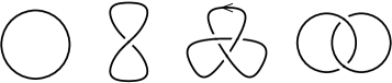
Figure 3.3: Shown from left to right are the unknot, another representation of the unknot, an oriented trefoil knot, and the Hopf link. Broken lines indicate undercrossings.

Reidemeister showed in 1927 that two knots are the same if and only if one can be deformed into the other by some sequence constructed from three elementary moves, known as the Reidemeister moves, shown in figure 3.4. This reduces the problem of distinguishing knots to a combinatorial problem, although one for which no efficient solution is known. In some cases, the sequence of Reidemeister moves needed to show equivalence of two knots involves intermediate steps that increase the number of crossings. Thus, it is very difficult to show upper bounds on the number of moves necessary. The most thoroughly studied knot equivalence problem is the problem of deciding whether a given knot is equivalent to the unknot. Even showing the decidability of this problem is highly nontrivial. This was achieved by Haken in 1961[87]. In 1998 it was shown by Hass, Lagarias, and Pippenger that the problem of recognizing the unknot is contained in NP[93].

Figure 3.4: Two knots are the same if and only if one can be deformed into the other by some sequence of the three Reidemeister moves shown above.

A knot invariant is any function on knots which is invariant under the Reidemeister moves. Thus, a knot invariant always takes the same value for different representations of the same knot, such as the two representations of the unknot shown in figure 3.3. In general, there can be distinct knots which a knot invariant fails to distinguish.

One of the best known knot invariants is the Jones polynomial, discovered in 1985 by Vaughan Jones[106]. To any oriented knot or link, it associates a Laurent polynomial in the variable $t^{1/2}$. The Jones polynomial has a degree in $t$ which grows at most linearly with the number of crossings in the link. The coefficients are all integers, but they may be exponentially large. Exact evaluation of Jones polynomials at all but a few special values of $t$ is #P-hard[101]. The Jones polynomial can be defined recursively by a simple “skein” relation. However, for our purposes it will be more convenient to use a definition in terms of a representation of the braid group, as discussed below.

Figure 3.5: Shown from left to right are a braid, its plat closure, and its trace closure.

To describe in more detail the computation of Jones polynomials we must specify how the knot will be represented on the computer. Although an embedding of a circle in $\mathbb{R}^{3}$ is a continuous object, all the topologically relevant information about a knot can be described in the discrete language of the braid group. Links can be constructed from braids by joining the free ends. Two ways of doing this are taking the plat closure and the trace closure, as shown in figure 3.5. Alexander’s theorem states that any link can be constructed as the trace closure of some braid. Any link can also be constructed as the plat closure of some braid. This can be easily proven as a corollary to Alexander’s theorem, as shown in figure 3.6.

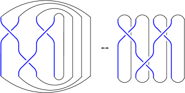
Figure 3.6: A trace closure of a braid on $n$ strands can be converted to a plat closure of a braid on $2n$ strands by moving the “return” strands into the braid.

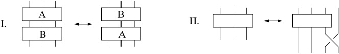
Figure 3.7: Shown are the two Markov moves. Here the boxes represent arbitrary braids. If a function on braids is invariant under these two moves, then the corresponding function on links induced by the trace closure is a link invariant.

Given that the trace closure provides a correspondence between links and braids, one may attempt to find functions on braids which yield link invariants via this correspondence. Markov’s theorem shows that a function on braids will yield a knot invariant provided it is invariant under the two Markov moves, shown in figure 3.7. Thus the Markov moves provide an analogue for braids of the Reidemeister moves on links. The constraints imposed by invariance under the Reidemeister moves are enforced in the braid picture jointly by invariance under Markov moves and by the defining relations of the braid group.

A linear function $f$ satisfying $f(AB)=f(BA)$ is called a trace. The ordinary trace on matrices is one such function. Taking a trace of a representation of the braid group yields a function on braids which is invariant under Markov move I. If the trace and representation are such that the resulting function is also invariant under Markov move II, then a link invariant will result. The Jones polynomial can be obtained in this way.

In [6], Aharonov, et al. show that an additive approximation to the Jones polynomial of the plat or trace closure of a braid at $t=e^{i2\pi/k}$ can be computed on a quantum computer in time which scales polynomially in the number of strands and crossings in the braid and in $k$. In [4, 174], it is shown that for plat closures, this problem is BQP-complete. The complexity of approximating the Jones polynomial for trace closures was left open, other than showing that it is contained in BQP.

The results of [6, 4, 174] reformulate and generalize the previous results of Freedman et al. [74, 73], which show that certain approximations of Jones polynomials are BQP-complete. The work of Freedman et al. in turn builds upon Witten’s discovery of a connection between Jones polynomials and topological quantum field theory [173]. Recently, Aharonov et al. have generalized further, obtaining an efficient quantum algorithm for approximating the Tutte polynomial for any planar graph, at any point in the complex plane, and also showing BQP-hardness at some points [5]. As special cases, the Tutte polynomial includes the Jones polynomial, other knot invariants such as the HOMFLY polynomial, and partition functions for some physical models such as the Potts model.

The algorithm of Aharonov et al. works by obtaining the Jones polynomial as a trace of the path model representation of the braid group. The path model representation is unitary for $t=e^{i2\pi/k}$ and, as shown in [6], can be efficiently implemented by quantum circuits. For computing the trace closure of a braid the necessary trace is similar to the ordinary matrix trace except that only a subset of the diagonal elements of the unitary implemented by the quantum circuit are summed, and there is an additional weighting factor. For the plat closure of a braid the computation instead reduces to evaluating a particular matrix element of the quantum circuit. Aharonov et al. also use the path model representation in their proof of BQP-completeness.

Given a braid $b$, we know that the problem of approximating the Jones polynomial of its plat closure is BQP-hard. By Alexander’s theorem, one can obtain a braid $b^{\prime}$ whose trace closure is the same link as the plat closure of $b$. The Jones polynomial depends only on the link, and not on the braid it was derived from. Thus, one may ask why this doesn’t immediately imply that estimating the Jones polynomial of the trace closure is a BQP-hard problem. The answer lies in the degree of approximation. As discussed in section 3.7, the BQP-complete problem for plat closures is to approximate the Jones polynomial to a certain precision which depends exponentially on the number of strands in the braid. The number of strands in $b^{\prime}$ can be larger than the number of strands in $b$, hence the degree of approximation obtained after applying Alexander’s theorem may be too poor to solve the original BQP-hard problem.

The fact that computing the Jones polynomial of the trace closure of a braid can be reduced to estimating a generalized trace of a unitary operator and the fact that trace estimation is DQC1-complete suggest a connection between Jones polynomials and the one clean qubit model. Here we find such a connection by showing that evaluating a certain approximation to the Jones polynomial of the trace closure of a braid at a fifth root of unity is DQC1-complete. The main technical difficulty is obtaining the Jones polynomial as a trace over the entire Hilbert space rather than as a summation of some subset of the diagonal matrix elements. To do this we will not use the path model representation of the braid group, but rather the Fibonacci representation, as described in the next section.

3.4 Fibonacci Representation

The Fibonacci representation $\rho_{F}^{(n)}$ of the braid group $B_{n}$ is described in [111] in the context of Temperley-Lieb recoupling theory. Temperley-Lieb recoupling theory describes two species of idealized “particles” denoted by $p$ and $*$. We will not delve into the conceptual and mathematical underpinnings of Temperley-Lieb recoupling theory. For present purposes, it will be sufficient to regard it as a formal procedure for obtaining a particular unitary representation of the braid group whose trace yields the Jones polynomial at $t=e^{i2\pi/5}$. Throughout most of this paper it will be more convenient to express the Jones polynomial in terms of $A=e^{-i3\pi/5}$, with $t$ defined by $t=A^{-4}$.

It is worth noting that the Fibonacci representation is a special case of the path model representation used in [6]. The path model representation applies when $t=e^{i2\pi/k}$ for any integer $k$, whereas the Fibonacci representation is for $k=5$. The relationship between these two representations is briefly discussed in section 3.10. However, for the sake of making our discussion self contained, we will derive all of our results directly within the Fibonacci representation.

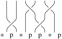
Figure 3.8: For an $n$-strand braid we can write a length $n+1$ string of $p$ and $*$ symbols across the base. The string may have no two $*$ symbols in a row, but can be otherwise arbitrary.

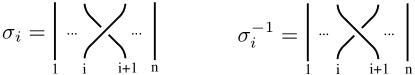
Figure 3.9: $\sigma_{i}$ denotes the elementary crossing of strands $i$ and $i+1$. The braid group on $n$ strands $B_{n}$ is generated by $\sigma_{1}\ldots\sigma_{n-1}$, which satisfy the relations $\sigma_{i}\sigma_{j}=\sigma_{j}\sigma_{i}$ for $|i-j|>1$ and $\sigma_{i+1}\sigma_{i}\sigma_{i+1}=\sigma_{i}\sigma_{i+1}\sigma_{i}$ for all $i$. The group operation corresponds to concatenation of braids.

Given an $n$-strand braid $b\in B_{n}$, we can write a length $n+1$ string of $p$ and $*$ symbols across the base as shown in figure 3.8. These strings have the restriction that no two $*$ symbols can be adjacent. The number of such strings is $f_{n+3}$, where $f_{n}$ is the $n^{\mathrm{th}}$ Fibonacci number, defined so that $f_{1}=1$, $f_{2}=1$, $f_{3}=2,\ldots$ Thus the formal linear combinations of such strings form an $f_{n+3}$-dimensional vector space. For each $n$, the Fibonacci representation $\rho_{F}^{(n)}$ is a homomorphism from $B_{n}$ to the group of unitary linear transformations on this space. We will describe the Fibonacci representation in terms of its action on the elementary crossings which generate the braid group, as shown in figure 3.9.

The elementary crossings correspond to linear operations which mix only those strings which differ by the symbol beneath the crossing. The linear transformations have a local structure, so that the coefficients for the symbol beneath the crossing to be changed or unchanged depend only on that symbol and its two neighbors. For example, using the notation of [111],

(3.3)

which means that the elementary crossing $\sigma_{i}$ corresponds to a linear transformation which takes any string whose $i^{\mathrm{th}}$ through $(i+2)^{\mathrm{th}}$ symbols are $p*p$ to the coefficient $c$ times the same string plus the coefficient $d$ times the same string with the $*$ at the $(i+1)^{\mathrm{th}}$ position replaced by $p$. (As shown in figure 9, the $i^{\mathrm{th}}$ crossing is over the $(i+1)^{\mathrm{th}}$ symbol.) To compute the linear transformation that the representation of a given braid applies to a given string of symbols, one can write the symbols across the base of the braid, and then apply rules of the form 3.3 until all the crossings are removed, and all that remains are various coefficients for different strings to be written across the base of a set of straight strands.

For compactness, we will use $(p\widehat{*}p)=c(p*p)+d(ppp)$ as a shorthand for equation 3.3. In this notation, the complete set of rules is as follows.

$$(*\widehat{p}p) = a(*pp)$$

$$(*\widehat{p}*) = b(*p*)$$

$$(p\widehat{*}p) = c(p*p)+d(ppp)$$

$$(p\widehat{p}*) = a(pp*)$$

$$(p\widehat{p}p) = d(p*p)+e(ppp),$$ (3.4)

where

$$a = -A^{4}$$

$$b = A^{8}$$

$$c = A^{8}\tau^{2}-A^{4}\tau$$

$$d = A^{8}\tau^{3/2}+A^{4}\tau^{3/2}$$

$$e = A^{8}\tau-A^{4}\tau^{2}$$

$$A = e^{-i3\pi/5}$$

$$\tau = 2/(1+\sqrt{5}).$$ (3.5)

Using these rules we can calculate any matrix from the Fibonacci representation of the braid group. Notice that this is a reducible representation. These rules do not allow the rightmost symbol or leftmost symbol of the string to change. Thus the vector space decomposes into four invariant subspaces, namely the subspace spanned by strings which begin and end with $p$, and the $*\ldots*$, $p\ldots*$, and $*\ldots p$ subspaces. As an example, we can use the above rules to compute the action of $B_{3}$ on the $*\ldots p$ subspace.

$$\rho_{*p}^{(3)}(\sigma_{1})=\left[\begin{array}[]{cc}b&0\\ 0&a\end{array}\right]\begin{array}[]{c}\textrm{$*$p$*$p}\\ \textrm{$*$ppp}\end{array}\quad\quad\quad\rho_{*p}^{(3)}(\sigma_{2})=\left[\begin{array}[]{cc}c&d\\ d&e\end{array}\right]\begin{array}[]{c}\textrm{$*$p$*$p}\\ \textrm{$*$ppp}\end{array}$$ (3.6)

In section 3.8 we prove that the Jones polynomial evaluated at $t=e^{i2\pi/5}$ can be obtained as a weighted trace of the Fibonacci representation over the $*\ldots*$ and $*\ldots p$ subspaces.

3.5 Computing the Jones Polynomial in DQC1

As mentioned previously, the Fibonacci representation acts on the vector space of formal linear combinations of strings of $p$ and $*$ symbols in which no two $*$ symbols are adjacent. The set of length $n$ strings of this type, $P_{n}$, has $f_{n+2}$ elements, where $f_{n}$ is the $n^{\mathrm{th}}$ Fibonacci number: $f_{1}=1$, $f_{2}=1$, $f_{3}=2$, and so on. As shown in section 3.12, one can construct a bijective correspondence between these strings and the integers from $0$ to $f_{n+2}-1$ as follows. If we think of $*$ as $1$ and $p$ as $0$, then with a string $s_{n}s_{n-1}\ldots s_{1}$ we associate the integer

$$z(s)=\sum_{i=1}^{n}s_{i}f_{i+1}.$$ (3.7)

This is known as the Zeckendorf representation.

Representing integers as bitstrings by the usual method of place value, we thus have a correspondence between the elements of $P_{n}$ and the bitstrings of length $b=\lceil\log_{2}(f_{n+2})\rceil$. This correspondence will be a key element in computing the Jones polynomial with a one clean qubit machine. Using a one clean qubit machine, one can compute the trace of a unitary over the entire Hilbert space of $2^{n}$ bitstrings. Using CNOT gates as above, one can also compute with polynomial overhead the trace over a subspace whose dimension is a polynomially large fraction of the dimension of the entire Hilbert space. However, it is probably not possible in general for a one clean qubit computer to compute the trace over subspaces whose dimension is an exponentially small fraction of the dimension of the total Hilbert space. For this reason, directly mapping the strings of $p$ and $*$ symbols to strings of $1$ and $0$ will not work. In contrast, the correspondence described in equation 3.7 maps $P_{n}$ to a subspace whose dimension is at least half the dimension of the full $2^{b}$-dimensional Hilbert space.

In outline, the DQC1 algorithm for computing the Jones polynomial works as follows. Using the results described in section 3.2, we will think of the quantum circuit as acting on $b$ maximally mixed qubits plus $O(1)$ clean qubits. Thinking in terms of the computational basis, we can say that the first $b$ qubits are in a uniform probabilistic mixture of the $2^{b}$ classical bitstring states. By equation 3.7, most of these bitstrings correspond to elements of $P_{n}$. In the Fibonacci representation, an elementary crossing on strands $i$ and $i-1$ corresponds to a linear transformation which can only change the value of the $i^{\mathrm{th}}$ symbol in the string of $p$’s and $*$’s. The coefficients for changing this symbol or leaving it fixed depend only on the two neighboring symbols. Thus, to simulate this linear transformation, we will use a quantum circuit which extracts the $(i-1)^{\mathrm{th}}$, $i^{\mathrm{th}}$, and $(i+1)^{\mathrm{th}}$ symbols from their bitstring encoding, writes them into an ancilla register while erasing them from the bitstring encoding, performs the unitary transformation prescribed by equation 3.4 on the ancillas, and then transfers this symbol back into the bitstring encoding while erasing it from the ancilla register. Constructing one such circuit for each crossing, multiplying them together, and performing DQC1 trace-estimation yields an approximation to the Jones polynomial.

Performing the linear transformation demanded by equation 3.4 on the ancilla register can be done easily by invoking gate set universality (cf. Solovay-Kitaev theorem [137]) since it is just a three-qubit unitary operation. The harder steps are transferring the symbol values from the bitstring encoding to the ancilla register and back.

It may be difficult to extract an arbitrary symbol from the bitstring encoding. However, it is relatively easy to extract the leftmost “most significant” symbol, which determines whether the Fibonacci number $f_{n}$ is present in the sum shown in equation 3.7. This is because, for a string $s$ of length $n$, $z(s)\geq f_{n-1}$ if and only if the leftmost symbol is $*$. Thus, starting with a clean $\left|{0}\right\rangle$ ancilla qubit, one can transfer the value of the leftmost symbol into the ancilla as follows. First, check whether $z(s)$ (as represented by a bitstring using place value) is $\geq f_{n-1}$. If so flip the ancilla qubit. Then, conditioned on the value of the ancilla qubit, subtract $f_{n-1}$ from the bitstring. (The subtraction will be done modulo $2^{b}$ for reversibility.)

Any classical circuit can be made reversible with only constant overhead. It thus corresponds to a unitary matrix which permutes the computational basis. This is the standard way of implementing classical algorithms on a quantum computer[137]. However, the resulting reversible circuit may require clean ancilla qubits as work space in order to be implemented efficiently. For a reversible circuit to be implementable on a one clean qubit computer, it must be efficiently implementable using at most logarithmically many clean ancillas. Fortunately, the basic operations of arithmetic and comparison for integers can all be done classically by NC1 circuits [171]. NC1 is the complexity class for problems solvable by classical circuits of logarithmic depth. As shown in [14], any classical NC1 circuit can be converted into a reversible circuit using only three clean ancillas. This is a consequence of Barrington’s theorem. Thus, the process described above for extracting the leftmost symbol can be done efficiently in DQC1.

More specifically, Krapchenko’s algorithm for adding two $n$-bit numbers has depth $\lceil\log n\rceil+O(\sqrt{\log n})$ [171]. A lower bound of depth $\log n$ is also known, so this is essentially optimal [171]. Barrington’s construction [20] yields a sequence of $2^{2d}$ gates on 3 clean ancilla qubits [14] to simulate a circuit of depth $d$. Thus we obtain an addition circuit which has quadratic size (up to a subpolynomial factor). Subtraction can be obtained analogously, and one can determine whether $a\geq b$ can be done by subtracting $a$ from $b$ and looking at whether the result is negative.

Although the construction based on Barrington’s theorem has polynomial overhead and is thus sufficient for our purposes, it seems worth noting that it is possible to achieve better efficiency. As shown by Draper [60], there exist ancilla-free quantum circuits for performing addition and subtraction, which succeed with high probability and have nearly linear size. Specifically, one can add or subtract a hardcoded number $a$ into an $n$-qubit register $\left|{x}\right\rangle$ modulo $2^{n}$ by performing quantum Fourier transform, followed by $O(n^{2})$ controlled-rotations, followed by an inverse quantum Fourier transform. Furthermore, using approximate quantum Fourier transforms[51, 19], [60] describes an approximate version of the circuit, which, for any value of parameter $m$, uses a total of only $O(mn\log n)$ gates to produce an output having an inner product with $\left|{x+a\mod 2^{n}}\right\rangle$ of $1-O(2^{-m})$.

Because they operate modulo $2^{n}$, Draper’s quantum circuits for addition and subtraction do not immediately yield fast ancilla-free quantum circuits for comparison, unlike the classical case. Instead, start with an $n$-bit number $x$ and then introduce a single clean ancilla qubit initialized to $\left|{0}\right\rangle$. Then subtract an $n$-bit hardcoded number $a$ from this register modulo $2^{n+1}$. If $a>x$ then the result will wrap around into the range $[2^{n},2^{n+1}-1]$, in which case the leading bit will be 1. If $a\leq x$ then the result will be in the range $[0,2^{n}-1]$. After copying the result of this leading qubit and uncomputing the subtraction, the comparison is complete. Alternatively, one could use the linear size quantum comparison circuit devised by Takahashi and Kunihiro, which uses $n$ uninitialized ancillas but no clean ancillas[163].

$$\begin{array}[]{cccc|cccccc}1&2&3&5&13&8&5&3&2&1\\ &p&p&*&p&p&*&p&p&p\end{array}\quad\leftrightarrow\quad(6,5)$$

Figure 3.10: Here we make a correspondence between strings of $p$ and $*$ symbols and ordered pairs of integers. The string of 9 symbols is split into substrings of length 4 and 5, and each one is used to compute an integer by adding the $(i+1)^{\mathrm{th}}$ Fibonacci number if $*$ appears in the $i^{\mathrm{th}}$ place. Note the two strings are read in different directions.

Unfortunately, most crossings in a given braid will not be acting on the leftmost strand. However, we can reduce the problem of extracting a general symbol to the problem of extracting the leftmost symbol. Rather than using equation 3.7 to make a correspondence between a string from $P_{n}$ and a single integer, we can split the string at some chosen point, and use equation 3.7 on each piece to make a correspondence between elements of $P_{n}$ and ordered pairs of integers, as shown in figure 3.10. To extract the $i^{\mathrm{th}}$ symbol, we thus convert encoding 3.7 to the encoding where the string is split between the $i^{\mathrm{th}}$ and $(i-1)^{\mathrm{th}}$ symbols, so that one only needs to extract the leftmost symbol of the second string. Like equation 3.7, this is also an efficient encoding, in which the encoded bitstrings form a large fraction of all possible bitstrings.

To convert encoding 3.7 to a split encoding with the split at an arbitrary point, we can move the split rightward by one symbol at a time. To introduce a split between the leftmost and second-to-leftmost symbols, one must extract the leftmost symbol as described above. To move the split one symbol to the right, one must extract the leftmost symbol from the right string, and if it is $*$ then add the corresponding Fibonacci number to the left string. This is again a procedure of addition, subtraction, and comparison of integers. Note that the computation of Fibonacci numbers in NC1 is not necessary, as these can be hardcoded into the circuits. Moving the split back to the left works analogously. As crossings of different pairs of strands are being simulated, the split is moved to the place that it is needed. At the end it is moved all the way leftward and eliminated, leaving a superposition of bitstrings in the original encoding, which have the correct coefficients determined by the Fibonacci representation of the given braid.

Lastly, we must consider the weighting in the trace, as described by equation 3.10. Instead of weight $W_{s}$, we will use $W_{s}/\phi$ so that the possible weights are 1 and $1/\phi$ both of which are $\leq 1$. We can impose any weight $\leq 1$ by doing a controlled rotation on an extra qubit. The CNOT trick for simulating a clean qubit which was described in section 3.2 can be viewed as a special case of this. All strings in which that qubit takes the value $\left|{1}\right\rangle$ have weight zero, as imposed by a $\pi/2$ rotation on the extra qubit. Because none of the weights are smaller than $1/\phi$, the weighting will cause only a constant overhead in the number of measurements needed to get a given precision.

3.6 DQC1-hardness of Jones Polynomials

We will prove DQC1-hardness of the problem of estimating the Jones polynomial of the trace closure of a braid by a reduction from the problem of estimating the trace of a quantum circuit. To do this, we will specify an encoding, that is, a map $\eta:Q_{n}\to S_{m}$ from the set $Q_{n}$ of strings of $p$ and $*$ symbols which start with $*$ and have no two $*$ symbols in a row, to $S_{m}$, the set of bitstrings of length $m$. For a given quantum circuit, we will construct a braid whose Fibonacci representation implements the corresponding unitary transformation on the encoded bits. The Jones polynomial of the trace closure of this braid, which is the trace of this representation, will equal the trace of the encoded quantum circuit.

Unlike in section 3.5, we will not use a one to one encoding between bit strings and strings of $p$ and $*$ symbols. All we require is that a sum over all strings of $p$ and $*$ symbols corresponds to a sum over bitstrings in which each bitstring appears an equal number of times. Equivalently, all bitstrings $b\in S_{m}$ must have a preimage $\eta^{-1}(b)$ of the same size. This insures an unbiased trace in which no bitstrings are overweighted. To achieve this we can divide the symbol string into blocks of three symbols and use the encoding

$$\begin{array}[]{ccc}\textrm{ppp}&\to&0\\ \textrm{p$*$p}&\to&1\\ \end{array}$$ (3.8)

The strings other than ppp and p$*$p do not correspond to any bit value. Since both the encoded 1 and the encoded 0 begin and end with p, they can be preceded and followed by any allowable string. Thus, changing an encoded 1 to an encoded zero does not change the number of allowed strings of $p$ and $*$ consistent with that encoded bitstring. Thus the condition that $|\eta^{-1}(b)|$ be independent of $b$ is satisfied.

We would also like to know a priori where in the string of p and $*$ symbols a given bit is encoded. This way, when we need to simulate a gate acting on a given bit, we would know which strands the corresponding braid should act on. If we were to simply divide our string of symbols into blocks of three and write down the corresponding bit string (skipping every block which is not in one of the two coding states ppp and p$*$p) then this would not be the case. Thus, to encode $n$ bits, we will instead divide the string of symbols into $n$ superblocks, each consisting of $c\log n$ blocks of three for some constant $c$. To decode a superblock, scan it from left to right until you reach either a ppp block or a p$*$p block. The first such block encountered determines whether the superblock encodes a 1 or a 0, according to equation 3.8. Now imagine we choose a string randomly from $Q_{3cn\log n}$. By choosing the constant prefactor $c$ in our superblock size we can ensure that in the entire string of $3cn\log n$ symbols, the probability of there being any noncoding superblock which contains neither a ppp block nor a p$*$p block is polynomially small. If this is the case, then these noncoding strings will contribute only a polynomially small additive error to the estimate of the circuit trace, on par with the other sources of error.

The gate set consisting of the CNOT, Hadamard, and $\pi/8$ gates is known to be universal for BQP [137]. Thus, it suffices to consider the simulation of 1-qubit and 2-qubit gates. Furthermore, it is sufficient to imagine the qubits arranged on a line and to allow 2-qubit gates to act only on neighboring qubits. This is because qubits can always be brought into neighboring positions by applying a series of SWAP gates to nearest neighbors. By our encoding a unitary gate applied to qubits $i$ and $i+1$ will correspond to a unitary transformation on symbols $i3c\log n$ through $(i+2)3c\log n-1$. The essence of our reduction is to take each quantum gate and represent it by a corresponding braid on logarithmically many symbols whose Fibonacci representation performs that gate on the encoded qubits.

Let’s first consider the problem of simulating a gate on the first pair of qubits, which are encoded in the leftmost two superblocks of the symbol string. We’ll subsequently consider the more difficult case of operating on an arbitrary pair of neighboring encoded qubits. As mentioned in section 3.4, the Fibonacci representation $\rho_{F}^{(n)}$ is reducible. Let $\rho_{**}^{(n)}$ denote the representation of the braid group $B_{n}$ defined by the action of $\rho_{F}^{(n)}$ on the vector space spanned by strings which begin and end with $*$. As shown in section 3.9, $\rho_{**}^{(n)}(B_{n})$ taken modulo phase is a dense subgroup of $SU(f_{n-1})$, and $\rho_{*p}^{(n)}(B_{n})$ modulo phase is a dense subgroup of $SU(f_{n})$.

In addition to being dense, the $**$ and $*$p blocks of the Fibonacci representation can be controlled independently. This is a consequence of the decoupling lemma, as discussed in section 3.9. Thus, given a string of symbols beginning with $*$, and any desired pair of unitaries on the corresponding $*$p and $**$ vector spaces, a braid can be constructed whose Fibonacci representation approximates these unitaries to any desired level of precision. However, the number of crossings necessary may in general be large. The space spanned by strings of logarithmically many symbols has only polynomial dimension. Thus, one might guess that the braid needed to approximate a given pair of unitaries on the $*$p and $**$ vector spaces for logarithmically many symbols will have only polynomially many crossings. It turns out that this guess is correct, as we state formally below.

Proposition 1.

Given any pair of elements $U_{*p}\in SU(f_{k+1})$ and $U_{**}\in SU(f_{k})$, and any real parameter $\epsilon$, one can in polynomial time find a braid $b\in B_{k}$ with $\mathrm{poly}(n,\log(1/\epsilon))$ crossings whose Fibonacci representation satisfies $\|\rho_{*p}(b)-U_{*p}\|\leq\epsilon$ and $\|\rho_{**}(b)-U_{**}\|\leq\epsilon$, provided that $k=O(\log n)$. By symmetry, the same holds when considering $\rho_{p*}$ rather than $\rho_{*p}$.

Note that proposition 1 is a property of the Fibonacci representation, not a generic consequence of density, since it is in principle possible for the images of group generators in a dense representation to lie exponentially close to some subgroup of the corresponding unitary group. We prove this proposition in section 3.11.

With proposition 1 in hand, it is apparent that any unitary gate on the first two encoded bits can be efficiently performed. To similarly simulate gates on arbitrary pairs of neighboring encoded qubits, we will need some way to unitarily bring a $*$ symbol to a known location within logarithmic distance of the relevant encoded qubits. This way, we ensure that we are acting in the $*p$ or $**$ subspaces.

To move $*$ symbols to known locations we’ll use an “inchworm” structure which brings a pair of $*$ symbols rightward to where they are needed. Specifically, suppose we have a pair of superblocks which each have a $*$ in their exact center. The presence of the left $*$ and the density of $\rho_{*p}$ allow us to use proposition 1 to unitarily move the right $*$ one superblock to the right by adding polynomially many crossings to the braid. Then, the presence of the right $*$ and the density of $\rho_{p*}$ allow us to similarly move the left $*$ one superblock to the right, thus bringing it into the superblock adjacent to the one which contains the right $*$. This is illustrated in figure 3.11. To move the inchworm to the left we use the inverse operation.

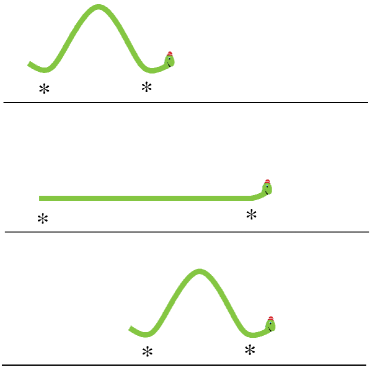
Figure 3.11: This sequence of unitary steps is used to bring a $*$ symbol where it is needed in the symbol string to ensure density of the braid group representation. The presence of the left $*$ ensures density to allow the movement of the right $*$ by proposition 1. Similarly, the presence of the right $*$ allows the left $*$ to be moved.

To simulate a given gate, one first uses the previously described procedure to make the inchworm crawl to the superblocks just to the left of the superblocks which encode the qubits on which the gate acts. Then, by the density of $\rho_{*p}$ and proposition 1, the desired gate can be simulated using polynomially many braid crossings.

To get this process started, the leftmost two superblocks must each contain a $*$ at their center. This occurs with constant probability. The strings in which this is not the case can be prevented from contributing to the trace by a technique analogous to that used in section 3.2 to simulate logarithmically many clean ancillas. Namely, an extra encoded qubit can be conditionally flipped if the first two superblocks do not both have $*$ symbols at their center. This can always be done using proposition 1, since the leftmost symbol in the string is always $*$, and the $\rho_{*p}$ and $\rho_{**}$ representations are both dense.

It remains to specify the exact unitary operations which move the inchworm. Suppose we have a current superblock and a target superblock. The current superblock contains a $*$ in its center, and the target superblock is the next superblock to the right or left. We wish to move the $*$ to the center of the target superblock. To do this, we can select the smallest segment around the center such that in each of these superblocks, the segment is bordered on its left and right by p symbols. This segment can then be swapped, as shown in figure 3.12.

Figure 3.12: This unitary procedure starts with a $*$ in the current superblock and brings it to the center of the target superblock.

For some possible strings this procedure will not be well defined. Specifically there may not be any segment which contains the center and which is bordered by p symbols in both superblocks. On such strings we define the operation to act as the identity. For random strings, the probability of this decreases exponentially with the superblock size. Thus, by choosing $c$ sufficiently large we can make this negligible for the entire computation.

As the inchworm moves rightward, it leaves behind a trail. Due to the swapping, the superblocks are not in their original state after the inchworm has passed. However, because the operations are unitary, when the inchworm moves back to the left, the modifications to the superblocks get undone. Thus the inchworm can shuttle back and forth, moving where it is needed to simulate each gate, always stopping just to the left of the superblocks corresponding to the encoded qubits.

The only remaining detail to consider is that the trace appearing in the Jones polynomial is weighted depending on whether the last symbol is $p$ or $*$, whereas the DQC1-complete trace estimation problem is for completely unweighted traces. This problem is easily solved. Just introduce a single extra superblock at the end of the string. After bringing the inchworm adjacent to the last superblock, apply a unitary which performs a conditional rotation on the qubit encoded by this superblock. The rotation will be by an angle so that the inner product of the rotated qubit with its original state is $1/\phi$ where $\phi$ is the golden ratio. This will be done only if the last symbol is $p$. This exactly cancels out the weighting which appears in the formula for the Jones polynomial, as described in section 3.8.

Thus, for appropriate $\epsilon$, approximating the Jones polynomial of the trace closure of a braid to within $\pm\epsilon$ is DQC1-hard.

3.7 Conclusion

The preceding sections show that the problem of approximating the Jones polynomial of the trace closure of a braid with $n$ strands and $m$ crossings to within $\pm\epsilon$ at $t=e^{i2\pi/5}$ is a DQC1-complete problem for appropriate $\epsilon$. The proofs are based on the problem of evaluating the Markov trace of the Fibonacci representation of a braid to $\frac{1}{\mathrm{poly}(n,m)}$ precision. By equation 3.11, we see that this corresponds to evaluating the Jones polynomial with $\pm\frac{|D^{n-1}|}{\mathrm{poly}(n,m)}$ precision, where $D=-A^{2}-A^{-2}=2\cos(6\pi/5)$. Whereas approximating the Jones polynomial of the plat closure of a braid was known[4] to be BQP-complete, it was previously only known that the problem of approximating the Jones polynomial of the trace closure of a braid was in BQP. Understanding the complexity of approximating the Jones polynomial of the trace closure of a braid to precision $\pm\frac{|D^{n-1}|}{\mathrm{poly}(n,m)}$ was posed as an open problem in [6]. This paper shows that for $A=e^{-i3\pi/5}$, this problem is DQC1-complete. Such a completeness result improves our understanding of both the difficulty of the Jones polynomial problem and the power one clean qubit computers by finding an equivalence between the two.

It is generally believed that DQC1 is not contained in P and does not contain all of BQP. The DQC1-completeness result shows that if this belief is true, it implies that approximating the Jones polynomial of the trace closure of a braid is not so easy that it can be done classically in polynomial time, but is not so difficult as to be BQP-hard.

To our knowledge, the problem of approximating the Jones polynomial of the trace closure of a braid is one of only four known candidates for classically intractable problems solvable on a one clean qubit computer. The others are estimating the Pauli decomposition of the unitary matrix corresponding to a polynomial-size quantum circuit, [118, 158], estimating quadratically signed weight enumerators[119], and estimating average fidelity decay of quantum maps[144, 153].

3.8 Jones Polynomials by Fibonacci Representation

For any braid $b\in B_{n}$ we will define $\widetilde{\mathrm{Tr}}(b)$ by:

$$\widetilde{\mathrm{Tr}}(b)=\frac{1}{\phi f_{n}+f_{n-1}}\sum_{s\in Q_{n+1}}W_{s}\begin{array}[]{l}\includegraphics[width=14.45377pt]{braidtrace.eps}\end{array}$$ (3.9)

We will use $\mid$ to denote a strand and $\nmid$ to denote multiple strands of a braid (in this case $n$). $Q_{n+1}$ is the set of all strings of $n+1$ $p$ and $*$ symbols which start with $*$ and contain no two $*$ symbols in a row. The symbol

$$\begin{array}[]{l}\includegraphics[width=14.45377pt]{braidtrace.eps}\end{array}$$

denotes the $s,s$ matrix element of the Fibonacci representation of braid $b$. The weight $W_{s}$ is

$$W_{s}=\left\{\begin{array}[]{ll}\phi&\textrm{if $s$ ends with $p$}\\ 1&\textrm{if $s$ ends with $*$}.\end{array}\right.$$ (3.10)

$\phi$ is the golden ratio $(1+\sqrt{5})/\sqrt{2}$.

As discussed in [6], the Jones polynomial of the trace closure of a braid $b$ is given by

$$V_{b^{\mathrm{tr}}}(A^{-4})=(-A)^{3w(b^{\mathrm{tr}})}D^{n-1}\mathrm{Tr}(\rho_{A}(b^{\mathrm{tr}})).$$ (3.11)

$b^{\mathrm{tr}}$ is the link obtained by taking the trace closure of braid $b$. $w(b^{\mathrm{tr}})$ is denotes the writhe of the link $b^{\mathrm{tr}}$. For an oriented link, one assigns a value of $+1$ to each crossing of the form , and the value $-1$ to each crossing of the form . The writhe of a link is defined to be the sum of these values over all crossings. $D$ is defined by $D=-A^{2}-A^{-2}$. $\rho_{A}:B_{n}\to\mathrm{TL}_{n}(D)$ is a representation from the braid group to the Temperley-Lieb algebra with parameter $D$. Specifically,

$$\rho_{A}(\sigma_{i})=AE_{i}+A^{-1}\mathds{1}$$ (3.12)

where $E_{1}\ldots E_{n}$ are the generators of $\mathrm{TL}_{n}(D)$, which satisfy the following relations.

$$E_{i}E_{j} = E_{j}E_{i}\quad\textrm{ for }|i-j|>1$$ (3.13)

$$E_{i}E_{i\pm 1}E_{i} = E_{i}$$ (3.14)

$$E_{i}^{2} = DE_{i}$$ (3.15)

The Markov trace on $\mathrm{TL}_{n}(D)$ is a linear map $\mathrm{Tr}:\mathrm{TL}_{n}(D)\to\mathbb{C}$ which satisfies

$$\mathrm{Tr}(\mathds{1}) = 1$$ (3.16)

$$\mathrm{Tr}(XY) = \mathrm{Tr}(YX)$$ (3.17)

$$\mathrm{Tr}(XE_{n-1}) = \frac{1}{D}\mathrm{Tr}(X^{\prime})$$ (3.18)

On the left hand side of equation 3.18, the trace is on $\mathrm{TL}_{n}(D)$, and $X$ is an element of $\mathrm{TL}_{n}(D)$ not containing $E_{n-1}$. On the right hand side of equation 3.18, the trace is on $\mathrm{TL}_{n-1}(D)$, and $X^{\prime}$ is the element of $\mathrm{TL}_{n-1}(D)$ which corresponds to $X$ in the obvious way since $X$ does not contain $E_{n-1}$.

We’ll show that the Fibonacci representation satisfies the properties implied by equations 3.12, 3.13, 3.14, and 3.15. We’ll also show that $\widetilde{\mathrm{Tr}}$ on the Fibonacci representation satisfies the properties corresponding to 3.16, 3.17, and 3.18. It was shown in [6] that properties 3.16, 3.17, and 3.18, along with linearity, uniquely determine the map $\mathrm{Tr}$. It will thus follow that $\widetilde{\mathrm{Tr}}(\rho_{F}^{(n)}(b))=\mathrm{Tr}(\rho_{A}(b))$, which proves that the Jones polynomial is obtained from the trace $\widetilde{\mathrm{Tr}}$ of the Fibonacci representation after multiplying by the appropriate powers of $D$ and $(-A)$ as shown in equation 3.11. Since these powers are trivial to compute, the problem of approximating the Jones polynomial at $A=e^{-i3\pi/5}$ reduces to the problem of computing this trace.

$\widetilde{\mathrm{Tr}}$ is equal to the ordinary matrix trace on the subspace of strings ending in $*$ plus $\phi$ times the matrix trace on the subspace of strings ending in p. Thus the fact that the matrix trace satisfies property 3.17 immediately implies that $\widetilde{\mathrm{Tr}}$ does too. Furthermore, since the dimensions of these subspaces are $f_{n-1}$ and $f_{n}$ respectively, we see from equation 3.9 that $\widetilde{\mathrm{Tr}}(\mathds{1})=1$. To address property 3.18, we’ll first show that

$$\widetilde{\mathrm{Tr}}\left(\begin{array}[]{l}\includegraphics[width=36.135pt]{braidbox3.eps}\end{array}\right)=\frac{1}{\delta}\widetilde{\mathrm{Tr}}\left(\begin{array}[]{l}\includegraphics[width=21.68121pt]{blanktrace2.eps}\end{array}\right)$$ (3.19)

for some constant $\delta$ which we will calculate. We will then use equation 3.12 to relate $\delta$ to $D$.

Using the definition of $\widetilde{\mathrm{Tr}}$ we obtain

$$\widetilde{\mathrm{Tr}}\left(\begin{array}[]{l}\includegraphics[width=36.135pt]{braidbox3.eps}\end{array}\right) = \frac{1}{f_{n}\phi+f_{n-1}}\left[\phi\sum_{s\in Q_{n-2}}\begin{array}[]{l}\includegraphics[width=36.135pt]{psp.eps}\end{array}+\phi\sum_{s\in Q_{n-2}}\begin{array}[]{l}\includegraphics[width=36.135pt]{ppp.eps}\end{array}\right.$$

$$\left.+\sum_{s\in Q_{n-2}}\begin{array}[]{l}\includegraphics[width=36.135pt]{pps.eps}\end{array}+\sum_{s\in Q^{\prime}_{n-2}}\begin{array}[]{l}\includegraphics[width=36.135pt]{sps.eps}\end{array}+\phi\sum_{s\in Q^{\prime}_{n-2}}\begin{array}[]{l}\includegraphics[width=36.135pt]{spp.eps}\end{array}\right]$$

where $Q^{\prime}_{n-2}$ is the set of length $n-2$ strings of $*$ and $p$ symbols which begin with $*$, end with $p$, and have no two $*$ symbols in a row.

Next we expand according to the braiding rules described in equations 3.3 and 3.4.

$$= \frac{1}{f_{n}\phi+f_{n-1}}\left[\sum_{s\in Q_{n-2}}\left(\phi c\begin{array}[]{l}\includegraphics[width=36.135pt]{straight_psp.eps}\end{array}+\phi e\begin{array}[]{l}\includegraphics[width=36.135pt]{straight_ppp.eps}\end{array}+a\begin{array}[]{l}\includegraphics[width=36.135pt]{straight_pps.eps}\end{array}\right)\right.$$

$$\left.+\sum_{s\in Q^{\prime}_{n-2}}\left(b\begin{array}[]{l}\includegraphics[width=36.135pt]{straight_sps.eps}\end{array}+\phi a\begin{array}[]{l}\includegraphics[width=36.135pt]{straight_spp.eps}\end{array}\right)\right]$$

We know that matrix elements in which differing string symbols are separated by unbraided strands will be zero. To obtain the preceding expression we have omitted such terms. Simplifying yields

$$=\frac{1}{f_{n}+\phi f_{n-1}}\left[\sum_{s\in Q_{n-2}}\left(\phi c\begin{array}[]{l}\includegraphics[width=25.29494pt]{ps.eps}\end{array}+(\phi e+a)\begin{array}[]{l}\includegraphics[width=25.29494pt]{pp.eps}\end{array}\right)+\sum_{s\in Q^{\prime}_{n-2}}(b+\phi a)\begin{array}[]{l}\includegraphics[width=25.29494pt]{sp.eps}\end{array}\right].$$

By the definitions of $A$, $a$, $b$, and $e$, given in equation 3.4, we see that $\phi e+a=b+\phi a$. Thus the above expression simplifies to

$$=\frac{1}{f_{n}\phi+f_{n-1}}\left[\sum_{s\in Q^{\prime}_{n-1}}\phi c\begin{array}[]{l}\includegraphics[width=21.68121pt]{s.eps}\end{array}+\sum_{s\in Q_{n-1}}(\phi e+a)\begin{array}[]{l}\includegraphics[width=21.68121pt]{p.eps}\end{array}\right]$$

Now we just need to show that

$$\frac{\phi c}{f_{n}\phi+f_{n-1}}=\frac{1}{\delta}\frac{1}{f_{n-1}\phi+f_{n-2}}$$ (3.24)

and

$$\frac{\phi e+a}{f_{n}\phi+f_{n-1}}=\frac{1}{\delta}\frac{\phi}{f_{n-1}\phi+f_{n-2}}.$$ (3.25)

The Fibonacci numbers have the property

$$\frac{f_{n}\phi+f_{n-1}}{f_{n-1}\phi+f_{n-2}}=\phi$$

for all $n$. Thus equations 3.24 and 3.25 are equivalent to

$$\phi c=\frac{1}{\delta}\phi$$ (3.26)

and

$$\phi e+a=\frac{1}{\delta}\phi^{2}$$ (3.27)

respectively. For $A=e^{-i3\pi/5}$ these both yield $\delta=A-1$. Hence

$$\widetilde{\mathrm{Tr}}\left(\begin{array}[]{l}\includegraphics[width=36.135pt]{braidbox3.eps}\end{array}\right)=\frac{1}{\delta}\frac{1}{f_{n-1}\phi+f_{n-2}}\left[\sum_{s\in Q^{\prime}_{n-1}}\begin{array}[]{l}\includegraphics[width=21.68121pt]{s.eps}\end{array}+\sum_{s\in Q_{n-1}}\phi\begin{array}[]{l}\includegraphics[width=21.68121pt]{p.eps}\end{array}\right]$$

$$=\frac{1}{\delta}\widetilde{\mathrm{Tr}}(b),$$

thus confirming equation 3.19.

Now we calculate $D$ from $\delta$. Solving 3.12 for $E_{i}$ yields

$$E_{i}=A^{-1}\rho_{A}(\sigma_{i})-A^{-2}\mathds{1}$$ (3.28)

Substituting this into 3.18 yields

$$\mathrm{Tr}(X(A^{-1}\rho_{A}(\sigma_{i})-A^{-2}\mathds{1}))=\frac{1}{D}\mathrm{Tr}(X)$$

$$\Rightarrow A^{-1}\mathrm{Tr}(X\rho_{A}(\sigma_{i}))-A^{-2}\mathrm{Tr}(X)=\frac{1}{D}\mathrm{Tr}(X).$$

Comparison to our relation $\mathrm{Tr}(X\rho_{A}(\sigma_{i}))=\frac{1}{\delta}\mathrm{Tr}(X)$ yields

$$A^{-1}\frac{1}{\delta}-A^{-2}=\frac{1}{D}.$$

Solving for $D$ and substituting in $A=e^{-i3\pi/5}$ yields

$$D=\phi.$$

This is also equal to $-A^{2}-A^{-2}$ consistent with the usage elsewhere.

Thus we have shown that $\widetilde{\mathrm{Tr}}$ has all the necessary properties. We will next show that the image of the representation $\rho_{F}$ of the braid group $B_{n}$ also forms a representation of the Temperley-Lieb algebra $TL_{n}(D)$. Specifically, $E_{i}$ is represented by

$$E_{i}\to A^{-1}\rho_{F}^{(n)}(\sigma_{i})-A^{-2}\mathds{1}.$$ (3.29)

To show that this is a representation of $TL_{n}(D)$ we must show that the matrices described in equation 3.29 satisfy the properties 3.13, 3.14, and 3.15. By the theorem of [6] which shows that a Markov trace on any representation of the Temperley-Lieb algebra yields the Jones polynomial, it will follow that the trace of the Fibonacci representation yields the Jones polynomial.

Since $\rho_{F}$ is a representation of the braid group and $\sigma_{i}\sigma_{j}=\sigma_{j}\sigma_{i}$ for $|i-j|>1$, it immediately follows that the matrices described in equation 3.29 satisfy condition 3.13. Next, we’ll consider condition 3.15. By inspection of the Fibonacci representation as given by equation 3.4, we see that by appropriately ordering the basis we can bring $\rho_{A}(\sigma_{i})$ into block diagonal form, where each block is one of the following $1\times 1$ or $2\times 2$ possibilities.

$$\left[a\right]\quad\left[b\right]\quad\left[\begin{array}[]{cc}c&d\\ d&e\end{array}\right]$$

Thus, by equation 3.29, it suffices to show that

$$\left(A^{-1}\left[\begin{array}[]{cc}c&d\\ d&e\end{array}\right]-A^{-2}\left[\begin{array}[]{cc}1&0\\ 0&1\end{array}\right]\right)^{2}=D\left(A^{-1}\left[\begin{array}[]{cc}c&d\\ d&e\end{array}\right]-A^{-2}\left[\begin{array}[]{cc}1&0\\ 0&1\end{array}\right]\right),$$

$$(A^{-1}a-A^{-2})^{2}=D(A^{-1}a-A^{-2}),$$

and

$$(A^{-1}b-A^{-2})^{2}=D(A^{-1}b-A^{-2}),$$

i.e. each of the blocks square to $D$ times themselves. These properties are confirmed by direct calculation.

Now all that remains is to check that the correspondence 3.29 satisfies property 3.14. Using the rules described in equation 3.4 we have

$$\rho_{F}^{(3)}(\sigma_{1})=\left[\begin{array}[]{cccccccc}b&0&&&&&&\\ 0&a&&&&&&\\ &&a&&&&&\\ &&&e&0&d&&\\ &&&0&a&0&&\\ &&&d&0&c&&\\ &&&&&&e&d\\ &&&&&&d&c\end{array}\right]\begin{array}[]{c}\textrm{$*$p$*$p}\\ \textrm{$*$ppp}\\ \textrm{$*$pp$*$}\\ \textrm{pppp}\\ \textrm{pp$*$p}\\ \textrm{p$*$pp}\\ \textrm{ppp$*$}\\ \textrm{p$*$p$*$}\\ \end{array}\quad\quad\rho_{F}^{(3)}(\sigma_{2})=\left[\begin{array}[]{cccccccc}c&d&&&&&&\\ d&e&&&&&&\\ &&a&&&&&\\ &&&e&d&0&&\\ &&&d&c&0&&\\ &&&0&0&a&&\\ &&&&&&a&0\\ &&&&&&0&b\end{array}\right]\begin{array}[]{c}\textrm{$*$p$*$p}\\ \textrm{$*$ppp}\\ \textrm{$*$pp$*$}\\ \textrm{pppp}\\ \textrm{pp$*$p}\\ \textrm{p$*$pp}\\ \textrm{ppp$*$}\\ \textrm{p$*$p$*$}\\ \end{array}$$

(Here we have considered all four subspaces unlike in equation 3.6.) Substituting this into equation 3.29 yields matrices which satisfy condition 3.15. It follows that equation 3.29 yields a representation of the Temperley-Lieb algebra. This completes the proof that

$$V_{b^{\mathrm{tr}}}(A^{-4})=(-A)^{3w(b^{\mathrm{tr}})}D^{n-1}\widetilde{\mathrm{Tr}}(\rho_{F}^{(n)}(b^{\mathrm{tr}}))$$

for $A=e^{-i3\pi/5}$.

3.9 Density of the Fibonacci representation

In this section we will show that $\rho_{**}^{(n)}(B_{n})$ is a dense subgroup of $SU(f_{n-1})$ modulo phase, and that $\rho_{*p}^{(n)}(B_{n})$ and $\rho_{p*}^{(n)}(B_{n})$ are dense subgroups of $SU(f_{n})$ modulo phase. Similar results regarding the path model representation of the braid group were proven in [4]. Our proofs will use many of the techniques introduced there.

We’ll first show that $\rho_{**}^{(4)}(B_{4})$ modulo phase is a dense subgroup of $SU(2)$. We can then use the bridge lemma from [4] to extend the result to arbitrary $n$.

Proposition 2.

$\rho_{**}^{(4)}(B_{4})$ modulo phase is a dense subgroup of $SU(2)$.

Proof.

Using equation 3.4 we have:

$$\rho_{**}^{(4)}(\sigma_{1})=\rho_{**}^{(4)}(\sigma_{3})=\left[\begin{array}[]{cc}b&0\\ 0&a\end{array}\right]\begin{array}[]{c}\textrm{$*$p$*$p$*$}\\ \textrm{$*$ppp$*$}\end{array}\quad\quad\rho_{**}^{(4)}(\sigma_{2})=\left[\begin{array}[]{cc}c&d\\ d&e\end{array}\right]\begin{array}[]{c}\textrm{$*$p$*$p$*$}\\ \textrm{$*$ppp$*$}\end{array}$$

We do not care about global phase so we will take

$$\rho_{**}^{(n)}(\sigma_{i})\quad\to\quad\frac{1}{\left(\det\rho_{**}^{(n)}(\sigma_{i})\right)^{1/f_{n-1}}}\ \rho_{**}^{(n)}(\sigma_{i})$$

to project into $SU(f_{n-1})$. Thus we must show the group $\langle A,B\rangle$ generated by

$$A=\frac{1}{\sqrt{ab}}\left[\begin{array}[]{cc}b&0\\ 0&a\end{array}\right]\quad\quad B=\frac{1}{\sqrt{ce-d^{2}}}\left[\begin{array}[]{cc}c&d\\ d&e\end{array}\right]$$ (3.30)

is a dense subgroup of $SU(2)$. To do this we will use the well known surjective homomorphism $\phi:SU(2)\to SO(3)$ whose kernel is $\{\pm\mathds{1}\}$ (cf. [15], pg. 276). A general element of $SU(2)$ can be written as

$$\cos\left(\frac{\theta}{2}\right)\mathds{1}+i\sin\left(\frac{\theta}{2}\right)\left[x\sigma_{x}+y\sigma_{y}+z\sigma_{z}\right]$$

where $\sigma_{x}$, $\sigma_{y}$, $\sigma_{z}$ are the Pauli matrices, and $x$, $y$, $z$ are real numbers satisfying $x^{2}+y^{2}+z^{2}=1$. $\phi$ maps this element to the rotation by angle $\theta$ about the axis

$$\vec{x}=\left[\begin{array}[]{c}x\\ y\\ z\end{array}\right].$$

Using equations 3.30 and 3.4, one finds that $\phi(A)$ and $\phi(B)$ are both rotations by $7\pi/5$. These rotations are about different axes which are separated by angle

$$\theta_{12}=\cos^{-1}(2-\sqrt{5})\simeq 1.8091137886\ldots$$

To show that $\rho_{**}^{(4)}(B_{4})$ modulo phase is a dense subgroup of $SU(2)$ it suffices to show that $\phi(A)$ and $\phi(B)$ generate a dense subgroup of $SO(3)$. To do this we take advantage of the fact that the finite subgroups of $SO(3)$ are completely known.

Theorem 3.

$\mathrm{(\cite[cite]{[\@@bibref{}{Artin}{}{}]}\ pg.\ 184)}$ Every finite subgroup of $SO(3)$ is one of the following:

• $C_{k}$: the cyclic group of order $k$

• $D_{k}$: the dihedral group of order $k$

• $T$: the tetrahedral group (order 12)

• $O$: the octahedral group (order 24)

• $I$: the icosahedral group (order 60)

The infinite proper subgroups of $SO(3)$ are all isomorphic to $O(2)$ or $SO(2)$. Thus, since $\phi(A)$ and $\phi(B)$ are rotations about different axes, $\langle\phi(A),\phi(B)\rangle$ can only be $SO(3)$ or a finite subgroup of $SO(3)$. If we can show that $\langle\phi(A),\phi(B)\rangle$ is not contained in any of the finite subgroups of $SO(3)$ then we are done.

Since $\phi(A)$ and $\phi(B)$ are rotations about different axes we know that $\langle\phi(A),\phi(B)\rangle$ is not $C_{k}$ or $D_{k}$. Next, we note that $R=\phi(A)^{5}\phi(B)^{5}$ is a rotation by $2\theta_{12}$. By direct calculation, $2\theta_{12}$ is not an integer multiple of $2\pi/k$ for $k=1,2,3,4,$ or 5. Thus $R$ has order greater than 5. As mentioned on pg. 262 of [105], $T$, $O$, and $I$ do not have any elements of order greater than 5. Thus, $\langle\phi(A),\phi(B)\rangle$ is not contained in $C$, $O$, or $I$, which completes the proof. Alternatively, using more arithmetic and less group theory, we can see that $2\theta_{12}$ is not any integer multiple of $2\pi/k$ for any $k\leq 30$, thus $R$ cannot be in $T$, $O$, or $I$ since its order does not divide the order of any of these groups. ∎

Next we’ll consider $\rho_{**}^{(n)}$ for larger $n$. These will be matrices acting on the strings of length $n+1$. These can be divided into those which end in pp$*$ and those which end in $*$p$*$. The space upon which $\rho_{**}^{(n)}$ acts can correspondingly be divided into two subspaces which are the span of these two sets of strings. From equation 3.4 we can see that $\rho_{**}^{(n)}(\sigma_{1})\ldots\rho_{**}^{(n)}(\sigma_{n-3})$ will leave these subspaces invariant. Thus if we order our basis to respect this grouping of strings, $\rho_{**}^{(n)}(\sigma_{1})\ldots\rho_{**}^{(n)}(\sigma_{n-3})$ will appear block-diagonal with a block corresponding to each of these subspaces.

The possible prefixes of $*$p$*$ are all strings of length $n-2$ that start with $*$ and end with p. Now consider the strings acted upon by $\rho_{**}^{(n-2)}$. These have length $n-1$ and must end in $*$. The possible prefixes of this $*$ are all strings of length $n-2$ that begin with $*$ and end with p. Thus these are in one to one correspondence with the strings acted upon by $\rho_{**}^{(n)}$ that end in $*$p$*$. Furthermore, since the rules 3.4 depend only on the three symbols neighboring a given crossing, the block of $\rho_{**}^{(n)}(\sigma_{1})\ldots\rho_{**}^{(n)}(\sigma_{n-3})$ corresponding to the $*$p$*$ subspace is exactly the same as $\rho_{**}^{(n-2)}(\sigma_{1})\ldots\rho_{**}^{(n-2)}(\sigma_{n-3})$. By a similar argument, the block of $\rho_{**}^{(n)}(\sigma_{1})\ldots\rho_{**}^{(n)}(\sigma_{n-3})$ corresponding to the pp$*$ is exactly the same as $\rho_{**}^{(n-1)}(\sigma_{1})\ldots\rho_{**}^{(n-1)}(\sigma_{n-3})$.

For any $n>3$, $\rho_{**}^{(n)}(\sigma_{n-2})$ will not leave these subspaces invariant. This is because the crossing $\sigma_{n-2}$ spans the $(n-1)^{\mathrm{th}}$ symbol. Thus if the $(n-2)^{\mathrm{th}}$ and $n^{\mathrm{th}}$ symbols are $p$, then by equation 3.4, $\rho_{**}^{(n)}$ can flip the value of the $(n-1)^{\mathrm{th}}$ symbol. The $n^{\mathrm{th}}$ symbol is guaranteed to be $p$, since the $(n+1)^{\mathrm{th}}$ symbol is the last one and is therefore $*$ by definition. For any $n>3$, the space acted upon by $\rho_{**}^{(n)}(\sigma_{n-1})$ will include some strings in which the $(n-2)^{\mathrm{th}}$ symbol is $p$.

As an example, for five strands:

$$\rho_{**}^{(5)}(\sigma_{1})=\left[\begin{array}[]{ccc}b&0&0\\ 0&a&0\\ 0&0&a\end{array}\right]\begin{array}[]{c}\textrm{$*$p$*$pp$*$}\\ \textrm{$*$pppp$*$}\\ \textrm{$*$pp$*$p$*$}\end{array}\quad\quad\rho_{**}^{(5)}(\sigma_{2})=\left[\begin{array}[]{ccc}c&d&0\\ d&e&0\\ 0&0&a\end{array}\right]\begin{array}[]{c}\textrm{$*$p$*$pp$*$}\\ \textrm{$*$pppp$*$}\\ \textrm{$*$pp$*$p$*$}\end{array}$$

$$\rho_{**}^{(5)}(\sigma_{3})=\left[\begin{array}[]{ccc}a&0&0\\ 0&e&d\\ 0&d&c\end{array}\right]\begin{array}[]{c}\textrm{$*$p$*$pp$*$}\\ \textrm{$*$pppp$*$}\\ \textrm{$*$pp$*$p$*$}\end{array}\quad\quad\rho_{**}^{(5)}(\sigma_{4})=\left[\begin{array}[]{ccc}a&0&0\\ 0&a&0\\ 0&0&b\end{array}\right]\begin{array}[]{c}\textrm{$*$p$*$pp$*$}\\ \textrm{$*$pppp$*$}\\ \textrm{$*$pp$*$p$*$}\end{array}$$

We recognize the upper $2\times 2$ blocks of $\rho_{**}^{(5)}(\sigma_{1})$, and $\rho_{**}^{(5)}(\sigma_{2})$ from equation 3.6. The lower $1\times 1$ block matches $\rho_{**}^{(3)}(\sigma_{1})$ and $\rho_{**}^{(3)}(\sigma_{2})$, which are both easily calculated to be $[a]$. $\rho_{**}^{(5)}(\sigma_{3})$ mixes these two subspaces.

We can now use the preceding observations about the recursive structure of $\{\rho_{**}^{(n)}|n=4,5,6,7\ldots\}$ to show inductively that $\rho_{**}^{(n)}(B_{n})$ forms a dense subgroup of $SU(f_{n-1})$ for all $n$. To perform the induction step we use the bridge lemma and decoupling lemma from [4].

Lemma 1 (Bridge Lemma).

Let $C=A\oplus B$ where $A$ and $B$ are vector spaces with $\dim{B}>\dim{A}\geq 1$. Let $W\in SU(C)$ be a linear transformation which mixes the subspaces $A$ and $B$. Then the group generated by $SU(A)$, $SU(B)$, and $W$ is dense in $SU(C)$.

Lemma 2 (Decoupling Lemma).

Let $G$ be an infinite discrete group, and let $A$ and $B$ be two vector spaces with $\dim(A)\neq\dim(B)$. Let $\rho_{a}:G\to SU(A)$ and $\rho_{b}:G\to SU(B)$ be homomorphisms such that $\rho_{a}(G)$ is dense in $SU(A)$ and $\rho_{b}(G)$ is dense in $SU(B)$. Then for any $U_{a}\in SU(A)$ there exist a series of $G$-elements $\alpha_{n}$ such that $\lim_{n\to\infty}\rho_{a}(\alpha_{n})=U_{a}$ and $\lim_{n\to\infty}\rho_{b}(\alpha_{n})=\mathds{1}$. Similarly, for any $U_{b}\in SU(B)$, there exists a series $\beta_{n}\in G$ such that $\lim_{n\to\infty}\rho_{a}(\beta_{n})=\mathds{1}$ and $\lim_{n\to\infty}\rho_{a}(\beta_{n})=U_{b}$.

With these in hand we can prove the main proposition of this section.

Proposition 3.

For any $n\geq 3$, $\rho_{**}^{(n)}(B_{n})$ modulo phase is a dense subgroup of $SU(f_{n-1})$.

Proof.

As mentioned previously, the proof will be inductive. The base cases are $n=3$ and $n=4$. As mentioned previously, $\rho_{**}^{(3)}(\sigma_{1})=\rho_{**}^{(3)}(\sigma_{2})=[a]$. Trivially, these generate a dense subgroup of (indeed, all of) $SU(1)=\{\mathds{1}\}$ modulo phase. By proposition 2, $\rho_{**}^{(4)}(\sigma_{1})$, and $\rho_{**}^{(4)}(\sigma_{2})$ generate a dense subgroup of $SU(2)$ modulo phase. Now for induction assume that $\rho_{**}^{(n-1)}(B_{n-1})$ is a dense subgroup of $SU(f_{n-2})$ and $\rho_{**}^{(n-2)}(B_{n-2})$ is a dense subgroup of $SU(f_{n-3})$. As noted above, these correspond to the upper and lower blocks of $\rho_{**}^{(n)}(\sigma_{1})\ldots\rho_{**}^{(n)}(\sigma_{n-2})$. Thus, by the decoupling lemma, $\rho_{**}^{(n)}(B_{n})$ contains an element arbitrarily close to $U\oplus\mathds{1}$ for any $U\in SU(f_{n-2})$ and an element arbitrarily close to $\mathds{1}\oplus U$ for any $U\in SU(f_{n-3})$. Since, as observed above, $\rho_{**}^{(n)}(\sigma_{n-1})$ mixes these two subspaces, the bridge lemma shows that $\rho_{**}^{(n)}(B_{n})$ is dense in $SU(f_{n-1})$. ∎

From this, the density of $\rho_{*p}^{(n)}$ and $\rho_{p*}^{(n)}$ easily follow.

Corollary 1.

$\rho_{*p}^{(n)}(B_{n})$ and $\rho_{p*}^{(n)}(B_{n})$ are dense subgroups of $SU(f_{n})$ modulo phase.

Proof.

It is not hard to see that

$$\begin{array}[]{rcl}\rho_{*p}^{(n)}(\sigma_{1})&=&\rho_{**}^{(n+1)}(\sigma_{1})\\ &\vdots&\\ \rho_{*p}^{(n)}(\sigma_{n-1})&=&\rho_{**}^{(n+1)}(\sigma_{n-1})\end{array}.$$

As we saw in the proof of proposition 3, $\rho_{**}^{(n+1)}(\sigma_{n})$ is not necessary to obtain density in $SU(f_{n})$, that is, $\langle\rho_{**}^{(n+1)}(\sigma_{1}),\ldots,\rho_{**}^{(n+1)}(\sigma_{n-1})\rangle$ is a dense subgroup of $SU(f_{n})$ modulo phase. Thus, the density of $\rho_{*p}^{(n)}$ in $SU(f_{n})$ follows immediately from the proof of proposition 3. By symmetry, $\rho_{p*}^{(n)}(B_{n})$ is isomorphic to $\rho_{*p}^{(n)}(B_{n})$, thus this is a dense subgroup of $SU(f_{n})$ modulo phase as well. ∎

3.10 Fibonacci and Path Model Representations

For any braid group $B_{n}$, and any root of unity $e^{i2\pi/k}$, the path model representation is a homomorphism from $B_{n}$ to to a set of linear operators. The vector space that these linear operators act is the space of formal linear combinations of $n$ step paths on the rungs of a ladder of height $k-1$ that start on the bottom rung. As an example, all the paths for $n=4$, $k=5$ are shown in below.

Thus, the $n=4,k=5$ path model representation is on a five dimensional vector space. For $k=5$ we can make a bijective correspondence between the allowed paths of $n$ steps and the set of strings of $p$ and $*$ symbols of length $n+1$ which start with $*$ and have no to $*$ symbols in a row. To do this, simply label the rungs from top to bottom as $*$, $p$, $p$, $*$, and directly read off the symbol string for each path as shown below.

In [6], it is explained in detail for any given braid how to calculate the corresponding linear transformation on paths. Using the correspondence described above, one finds that the path model representation for $k=5$ is equal to the $-1$ times Fibonacci representation described in this paper. This sign difference is a minor detail which arises only because [6] chooses a different fourth root of $t$ for $A$ than we do. This sign difference is automatically compensated for in the factor of $(-A)^{3\cdot\mathrm{writhe}}$, so that both methods yield the correct Jones polynomial.

3.11 Unitaries on Logarithmically Many Strands

In this section we’ll prove the following proposition.

Proposition 1.

Given any pair of elements $U_{*p}\in SU(f_{k+1})$ and $U_{**}\in SU(f_{k})$, and any real parameter $\epsilon$, one can in polynomial time find a braid $b\in B_{k}$ with $\mathrm{poly}(n,\log(1/\epsilon))$ crossings whose Fibonacci representation satisfies $\|\rho_{*p}(b)-U_{*p}\|\leq\epsilon$ and $\|\rho_{**}(b)-U_{**}\|\leq\epsilon$, provided that $k=O(\log n)$. By symmetry, the same holds when considering $\rho_{p*}$ rather than $\rho_{*p}$.

To do so, we’ll use a recursive construction. Suppose that we already know how to achieve proposition 1 on $n$ symbols, and we wish to extend this to $n+1$ symbols. Using the construction for $n$ symbols we can efficiently obtain a unitary of the form

$$M_{n-1}(A,B)=\begin{array}[]{l}\includegraphics[width=144.54pt]{inductblocks.eps}\end{array}$$ (3.31)

where $A$ and $B$ are arbitrary unitaries of the appropriate dimension. The elementary crossing $\sigma_{n}$ on the last two strands has the representation

$$M_{n}=\left[\begin{array}[]{ccccc}b&&&&\\ &a&&&\\ &&a&&\\ &&&e&d\\ &&&d&c\end{array}\right]\begin{array}[]{c}\textrm{$*$ \ldots$*$p$*$}\\ \textrm{$*$ \ldots pp$*$}\\ \textrm{$*$ \ldots$*$pp}\\ \textrm{$*$ \ldots ppp}\\ \textrm{$*$ \ldots p$*$p}\end{array}.$$

As a special case of equation 3.31, we can obtain

$$M_{\mathrm{diag}}(\alpha)=\left[\begin{array}[]{ccccc}e^{i\alpha/2}&&&&\\ &e^{i\alpha/2}&&&\\ &&e^{i\alpha/2}&&\\ &&&e^{i\alpha/2}&\\ &&&&e^{-i\alpha/2}\end{array}\right]\begin{array}[]{c}\textrm{$*$ \ldots$*$p$*$}\\ \textrm{$*$ \ldots pp$*$}\\ \textrm{$*$ \ldots$*$pp}\\ \textrm{$*$ \ldots ppp}\\ \textrm{$*$ \ldots p$*$p}\end{array}.$$

Where $0\leq\alpha<2\pi$. We’ll now show the following.

Lemma 3.

For any element

$$\left[\begin{array}[]{cc}V_{11}&V_{12}\\ V_{21}&V_{22}\end{array}\right]\in SU(2),$$

one can find some product $P$ of $O(1)$ $M_{\mathrm{diag}}$ matrices and $M_{n}$ matrices such that for some phases $\phi_{1}$ and $\phi_{2}$,

$$P=\left[\begin{array}[]{ccccc}\phi_{1}&&&&\\ &\phi_{2}&&&\\ &&\phi_{2}&&\\ &&&V_{11}&V_{12}\\ &&&V_{21}&V_{22}\end{array}\right]\begin{array}[]{c}\textrm{$*$ \ldots$*$p$*$}\\ \textrm{$*$ \ldots pp$*$}\\ \textrm{$*$ \ldots$*$pp}\\ \textrm{$*$ \ldots ppp}\\ \textrm{$*$ \ldots p$*$p}\end{array}.$$

Proof.

Let $B_{\mathrm{diag}}(\alpha)$ and $B_{n}$ be the following $2\times 2$ matrices

$$B_{\mathrm{diag}}(\alpha)=\left[\begin{array}[]{cc}e^{i\alpha/2}&0\\ 0&e^{-i\alpha/2}\end{array}\right]\quad\mathrm{and}\quad B_{n}=\left[\begin{array}[]{cc}e&d\\ d&c\end{array}\right]$$

We wish to show that we can approximate an arbitrary element of $SU(2)$ as a product of $O(1)$ $B_{\mathrm{diag}}$ and $B_{n}$ matrices. To do this, we will use the well known homomorphism $\phi:SU(2)\to SO(3)$ whose kernel is $\{\pm\mathds{1}\}$ (see section 3.9). To obtain an arbitrary element $V$ of $SU(2)$ modulo phase it suffices to show that the we can use $\phi(B_{n})$ and $\phi(B_{\mathrm{diag}}(\alpha))$ to obtain an arbitrary $SO(3)$ rotation. In section 3.9 we showed that

$$\left[\begin{array}[]{cc}a&0\\ 0&b\end{array}\right]\quad\mathrm{and}\quad\left[\begin{array}[]{cc}e&d\\ d&c\end{array}\right]$$

correspond to two rotations of $7\pi/5$ about axes which are separated by an angle of $\theta_{12}\simeq 1.8091137886\ldots$ By the definition of $\phi$, $\phi(B_{\mathrm{diag}}(\alpha))$ is a rotation by angle $\alpha$ about the same axis that $\phi\left(\left[\begin{array}[]{cc}a&0\\ 0&b\end{array}\right]\right)$ rotates about. $\phi(B_{n}^{5})$ is a $\pi$ rotation. Hence, $R(\alpha)\equiv\phi(B_{n}^{5}B_{\mathrm{diag}}(\alpha)B_{n}^{5})$ is a rotation by angle $\alpha$ about an axis which is separated by angle $2\theta_{12}-\pi$ from the axis that $\phi(B_{\mathrm{diag}}(\alpha))$ rotates about. $Q\equiv R(\pi)\phi(B_{\mathrm{diag}}(\alpha))R(\pi)$ is a rotation by angle $\alpha$ about some axis whose angle of separation from the axis that $\phi(B_{\mathrm{diag}}(\alpha))$ rotates about is $2(2\theta_{12}-\pi)\simeq 0.9532$. Similarly, by geometric visualization, $\phi(B_{\mathrm{diag}}(\alpha^{\prime}))Q\phi(B_{\mathrm{diag}}(-\alpha^{\prime}))$ is a rotation by $\alpha$ about an axis whose angle of separation from the axis that $Q$ rotates about is anywhere from $0$ to $2\times 0.9532$ depending on the value of $\alpha^{\prime}$. Since $2\times 0.9532>\pi/2$, there exists some choice of $\alpha^{\prime}$ such that this angle of separation is $\pi/2$. Thus, using the rotations we have constructed we can perform Euler rotations to obtain an arbitrary rotation. ∎

As a special case of lemma 3, we can obtain, up to global phase,

$$M_{\mathrm{swap}}=\left[\begin{array}[]{ccccc}\phi_{1}&&&&\\ &\phi_{2}&&&\\ &&\phi_{2}&&\\ &&&0&1\\ &&&1&0\end{array}\right]\begin{array}[]{c}\textrm{$*$ \ldots$*$p$*$}\\ \textrm{$*$ \ldots pp$*$}\\ \textrm{$*$ \ldots$*$pp}\\ \textrm{$*$ \ldots ppp}\\ \textrm{$*$ \ldots p$*$p}\end{array}.$$

Similarly, we can produce $M_{\mathrm{swap}}^{-1}$. Using $M_{\mathrm{swap}}$, $M_{\mathrm{swap}}^{-1}$, and equation 3.31 we can produce the matrix

$$M_{C}=\begin{array}[]{l}\includegraphics[width=144.54pt]{cblock.eps}\end{array}$$

for any unitary $C$. We do it as follows. Since $C$ is a normal operator, it can be unitarily diagonalized. That is, there exists some unitary $U$ such that $UCU^{-1}=D$ for some diagonal unitary $D$. Next, note that in equation 3.31 the dimension of $B$ is more than half that of $A$. Let $d=\mathrm{dim}(A)-\mathrm{dim}(B)$, and let $I_{d}$ be the identity operator of dimension $d$. We can easily construct two diagonal unitaries $D_{1}$ and $D_{2}$ of dimension $\mathrm{dim}(B)$ such that $(D_{1}\oplus I_{d})(I_{d}\oplus D_{2})=D$. As special cases of equation 3.31 we can obtain

$$M_{D_{1}}=\left[\begin{array}[]{ccccc}1&&&&\\ &1&&&\\ &&1&&\\ &&&1&\\ &&&&D_{1}\end{array}\right]\begin{array}[]{c}\textrm{$*$ \ldots$*$p$*$}\\ \textrm{$*$ \ldots pp$*$}\\ \textrm{$*$ \ldots$*$pp}\\ \textrm{$*$ \ldots ppp}\\ \textrm{$*$ \ldots p$*$p}\end{array}$$

and

$$M_{D_{2}}=\left[\begin{array}[]{ccccc}1&&&&\\ &1&&&\\ &&1&&\\ &&&1&\\ &&&&D_{2}\end{array}\right]\begin{array}[]{c}\textrm{$*$ \ldots$*$p$*$}\\ \textrm{$*$ \ldots pp$*$}\\ \textrm{$*$ \ldots$*$pp}\\ \textrm{$*$ \ldots ppp}\\ \textrm{$*$ \ldots p$*$p}\end{array}$$

and

$$M_{P}=\begin{array}[]{l}\includegraphics[width=144.54pt]{mpblocks.eps}\end{array}$$

where $P$ is a permutation matrix that shifts the lowest $\dim(B)$ basis states from the bottom of the block to the top of the block. Thus we obtain

$$M_{2}\equiv M_{\mathrm{swap}}M_{D_{2}}M_{\mathrm{swap}}^{-1}=\begin{array}[]{l}\includegraphics[width=144.54pt]{d2mat.eps}\end{array}$$

and

$$M_{1}\equiv M_{P}M_{\mathrm{swap}}M_{D_{1}}M_{\mathrm{swap}}^{-1}M_{P}^{-1}=\begin{array}[]{l}\includegraphics[width=144.54pt]{d1mat.eps}\end{array}.$$

Thus

$$M_{1}M_{2}=\begin{array}[]{l}\includegraphics[width=144.54pt]{idimat.eps}\end{array}.$$

As a special case of equation 3.31 we can obtain

$$M_{U}=\begin{array}[]{l}\includegraphics[width=144.54pt]{umat.eps}\end{array}.$$

Thus we obtain $M_{C}$ by the construction $M_{C}=M_{U}M_{1}M_{2}M_{U}^{-1}$. By multiplying together $M_{C}$ and $M_{n-1}$ we can control the three blocks independently. For arbitrary unitaries $A,B,C$ of appropriate dimension we can obtain

$$M_{ACB}=\begin{array}[]{l}\includegraphics[width=144.54pt]{acbmat.eps}\end{array}.$$ (3.32)

As a special case of equation 3.32 we can obtain

$$M_{\mathrm{unphase}}=\left[\begin{array}[]{ccccc}\phi_{1}^{*}&&&&\\ &\phi_{2}^{*}&&&\\ &&\phi_{2}^{*}&&\\ &&&1&\\ &&&&1\end{array}\right]\begin{array}[]{c}\textrm{$*$ \ldots$*$p$*$}\\ \textrm{$*$ \ldots pp$*$}\\ \textrm{$*$ \ldots$*$pp}\\ \textrm{$*$ \ldots ppp}\\ \textrm{$*$ \ldots p$*$p}\end{array}.$$

Thus, we obtain a clean swap

$$M_{\mathrm{clean}}=M_{\mathrm{unphase}}M_{\mathrm{swap}}=\left[\begin{array}[]{ccccc}1&&&&\\ &1&&&\\ &&1&&\\ &&&0&1\\ &&&1&0\end{array}\right]\begin{array}[]{c}\textrm{$*$ \ldots$*$p$*$}\\ \textrm{$*$ \ldots pp$*$}\\ \textrm{$*$ \ldots$*$pp}\\ \textrm{$*$ \ldots ppp}\\ \textrm{$*$ \ldots p$*$p}\end{array}.$$ (3.33)

We’ll now use $M_{\mathrm{clean}}$ and $M_{ACB}$ as our building blocks to create the maximally general unitary

$$M_{\mathrm{gen}}(V,W)=\begin{array}[]{l}\includegraphics[width=144.54pt]{genmat.eps}\end{array}.$$ (3.34)

For $n+1$ symbols, the $*\ldots*pp$ subspace has dimension $f_{n-3}$, and the $*\ldots p*p$ and $*\ldots ppp$ subspaces each have dimension $f_{n-2}$. Thus, in equation 3.32, the block $C$ has dimension $f_{n-2}+f_{n-3}=f_{n-1}$, and the block $B$ has dimension $f_{n-2}$. To construct $M_{\mathrm{gen}}(V,W)$ we will choose a subset of the $f_{n}$ basis states acted upon by the $B$ and $C$ blocks and permute them into the $C$ block. Then using $M_{ACB}$, we’ll perform an arbitrary unitary on these basis states. At each such step we can act upon a subspace whose dimension is a constant fraction of the dimension of the entire $f_{n}$ dimensional space on which we wish to apply an arbitrary unitary. Furthermore, this constant fraction is more than half. Specifically, $f_{n}/f_{n-1}\simeq 1/\phi\simeq 0.62$ for large $n$. We’ll show that an arbitrary unitary can be built up as a product of a constant number of unitaries each of which act only on half the basis states. Thus our ability to act on approximately $62\%$ of the basis states at each step is more than sufficient.

Before proving this, we’ll show how to permute an arbitrary set of basis states into the $C$ block of $M_{ACB}$. Just use $M_{\mathrm{clean}}$ to swap the $B$ block into the $*\ldots ppp$ subspace of the $C$ block. Then, as a special case of equation 3.32, choose $A$ and $B$ to be the identity, and $C$ to be a permutation which swaps some states between the $*\ldots*pp$ and $*\ldots ppp$ subspaces of the $C$ block. The states which we swap up from the $*\ldots ppp$ subspace are the ones from $B$ which we wish to move into $C$. The ones which we swap down from the $*\ldots*pp$ subspace are the ones from $C$ which we wish to move into $B$. This process allows us to swap a maximum of $f_{n-3}$ states between the $B$ block and the $C$ block. Since $f_{n-3}$ is more than half the dimension of the $B$ block, it follows that any desired permutation of states between the $B$ and $C$ blocks can be achieved using two repetitions of this process.

We’ll now show the following.

Lemma 4.

Let $m$ by divisible by 4. Any $m\times m$ unitary can be obtained as a product of seven unitaries, each of which act only on the space spanned by $m/2$ of the basis states, and leave the rest of the basis states undisturbed.

It will be obvious from the proof that even if the dimension of the matrix is not divisible by four, and the fraction of the basis states on which the individual unitaries act is not exactly $1/2$ it will still be possible to obtain an arbitrary unitary using a constant number of steps independent of $m$. Therefore, we will not explicitly work out this straightforward generalization.

Proof.

In [137] it is shown that for any unitary $U$, one can always find a series of unitaries $L_{n},\ldots,L_{1}$ which each act on only two basis states such that $L_{n}\ldots L_{1}U$ is the identity. Thus $L_{n}\ldots L_{1}=U^{-1}$. It follows that any unitary can be obtained as a product of such two level unitaries. The individual matrices $L_{1},\ldots,L_{n}$ each perform a (unitary) row operation on $U$. The sequence $L_{n}\ldots L_{1}$ reduces $U$ to the identity by a method very similar to Gaussian elimination. We will use a very similar construction to prove the present lemma. The essential difference is that we must perform the two level unitaries in groups. That is, we choose some set of $m/2$ basis states, perform a series of two level unitaries on them, then choose another set of $m/2$ basis states, perform a series of two level unitaries on them, and so on. After a finite number of such steps (it turns out that seven will suffice) we will reduce $U$ to the identity.

Our two-level unitaries will all be of the same type. We’ll fix our attention on two entries in $U$ taken from a particular column: $U_{ik}$ and $U_{jk}$. We wish to perform a unitary row operation, i.e. left multiply by a two level unitary, to set $U_{jk}=0$. If $U_{ik}$ and $U_{jk}$ are not both zero, then the two-level unitary which acts on the rows $i$ and $j$ according to

$$\frac{1}{\sqrt{|U_{ik}|^{2}+|U_{jk}|^{2}}}\left[\begin{array}[]{cc}U_{ik}^{*}&U_{jk}^{*}\\ U_{jk}&-U_{ik}\end{array}\right]$$ (3.35)

will achieve this. If $U_{ik}$ and $U_{jk}$ are both zero there is nothing to be done.

We can now use this two level operation within groups of basis states to eliminate matrix elements of $U$ one by one. As in Gaussian elimination, the key is that once you’ve obtained some zero matrix elements, your subsequent row operations must be chosen so that they do not make these nonzero again, undoing your previous work.

As the first step, we’ll act on the top $m/2$ rows in order to reduce the upper-left quadrant of $U$ to upper triangular form. We can do this as follows. Consider the first and second entries in the first column. Using the operation 3.35 we can make the second entry zero. Next consider the first and third entries in the first column. By operation 3.35 we can similarly make the third entry zero. Repeating this procedure, we get all of the entries in the top half of the first column to be zero other than the top entry. Next, we perform the same procedure on the second column except leaving out the top row. These row operations will not alter the first column since the rows being acted upon all have zero in the first column. We can then repeat this procedure for each column in the left half of $U$ until the upper-left block is upper triangular.

We’ll now think of U in terms of 16 blocks of size $(m/4)\times(m/4)$. In the second step we’ll eliminate the matrix elements in the third block of the first column. The second step is shown schematically as

$$\begin{array}[]{l}\includegraphics[width=144.54pt]{step2.eps}\end{array}$$

The curly braces indicate the rows to be acted upon, and the unshaded areas represent zero matrix elements. This step can be performed very similarly to the first step. The nonzero matrix elements in the bottom part of the first column can be eliminated one by one by interacting with the first row. The nonzero matrix elements in the bottom part of the second column can then be eliminated one by one by interacting with the second row. The first column will be undisturbed by this because the rows being acted upon in this step have zero matrix elements in the first column. Similarly acting on the remaining columns yields the desired result.

The next step, as shown below, is nearly identical and can be done the same way.

$$\begin{array}[]{l}\includegraphics[width=144.54pt]{step3.eps}\end{array}$$ (3.36)

The matrix on the right hand side of 3.36 is unitary. It follows that it must be of the form

$$\begin{array}[]{l}\includegraphics[width=50.58878pt]{matform.eps}\end{array}$$

where the upper-leftmost block is a diagonal unitary. We can next apply the same sorts of steps to the lower $3\times 3$ blocks, as illustrated below.

$$\begin{array}[]{l}\includegraphics[width=209.58255pt]{steps45.eps}\end{array}$$

By unitarity the resulting matrix is actually of the form

$$\begin{array}[]{l}\includegraphics[width=50.58878pt]{matform2.eps}\end{array}$$

where the lower-right quadrant is an $(m/2)\times(m/2)$ unitary matrix, and the upper-left quadrant is an $(m/2)\times(m/2)$ diagonal unitary matrix. We can now apply the inverse of the upper-left quadrant to the top $m/2$ rows and then apply the inverse of the lower-right quadrant to the bottom $m/2$ rows. This results in the identity matrix, and we are done. In total we have used seven steps. ∎

Examining the preceding construction, we can see the recursive step uses a constant number of the $M_{n-1}$ operators from the next lower level of recursion, plus a constant number of $M_{n}$ operators. Thus, the number of crossings in the braid grows only exponentially in the recursion depth. Since each recursion adds one more symbol, we see that to construct $M_{\mathrm{gen}}(V,W)$ on logarithmically many symbols requires only polynomially many crossings in the corresponding braid.

The main remaining task is to work out the base case on which the recursion rests. Since the base case is for a fixed set of generators on a fixed number of symbols, we can simply use the Solovay-Kitaev theorem[116].

Theorem 4 (Solovay-Kitaev).

Suppose matrices $U_{1},\ldots,U_{r}$ generate a dense subgroup in $SU(d)$. Then, given a desired unitary $U\in SU(d)$, and a precision parameter $\delta>0$, there is an algorithm to find a product $V$ of $U_{1},\ldots,U_{r}$ and their inverses such that $\|V-U\|\leq\delta$. The length of the product and the runtime of the algorithm are both polynomial in $\log(1/\delta)$.

Because the total complexity of the process is polynomial, it is only necessary to implement the base case to polynomially small $\delta$ in order for the final unitary $M_{\mathrm{gen}}(V,W)$ to have polynomial precision. This follows from simple error propagation. An analogous statement about the precision of gates needed in quantum circuits is worked out in [137]. This completes the proof of proposition 1.

3.12 Zeckendorf Representation

Following [111], to construct the Fibonacci representation of the braid group, we use strings of p and $*$ symbols such that no two $*$ symbols are adjacent. There exists a bijection $z$ between such strings and the integers, known as the Zeckendorf representation. Let $P_{n}$ be the set of all such strings of length $n$. To construct the map $z:P_{n}\to\{0,1,\ldots,f_{n+2}\}$ we think of $*$ as one and $p$ as zero. Then, for a given string $s=s_{n}s_{n-1}\ldots s_{1}$ we associate the integer

$$z(s)=\sum_{i=1}^{n}s_{i}f_{i+1},$$ (3.37)

where $f_{i}$ is the $i^{\mathrm{th}}$ Fibonacci number: $f_{1}=1,f_{2}=1,f_{3}=2$, and so on. In this section we’ll show the following.

Proposition 4.

For any $n$, the map $z:P_{n}\to\{0,\ldots,f_{n+2}\}$ defined by $z(s)=\sum_{i=1}^{n}s_{i}f_{i+1}$ is bijective.

Proof.

We’ll inductively show that the following two statements are true for every $n\geq 2$.

$\mathbf{A_{n}:}\quad$ $z$ maps strings of length $n$ starting with p bijectively to $\{0,\ldots,f_{n+1}-1\}$.

$\mathbf{B_{n}:}\quad$ $z$ maps strings of length $n$ starting with $*$ bijectively to $\{f_{n+1},\ldots,f_{n+2}-1\}$.

Together, $A_{n}$ and $B_{n}$ imply that $z$ maps $P_{n}$ bijectively to $\{0,\ldots,f_{n+2}-1\}$. As a base case, we can look at $n=2$.

$$pp \leftrightarrow 0$$

$$p* \leftrightarrow 1$$

$$p \leftrightarrow 2$$

Thus $A_{2}$ and $B_{2}$ are true. Now for the induction. Let $s_{n-1}\in P_{n-1}$. By equation 3.37,

$$z(ps_{n-1})=z(s_{n-1}).$$

Since $s_{n-1}$ follows a p symbol, it can be any element of $P_{n-1}$. By induction, $z$ is bijective on $P_{n-1}$, thus $A_{n}$ is true. Similarly, by equation 3.37

$$z(*s_{n-1})=f_{n+1}+z(s_{n-1}).$$

Since $s_{n-1}$ here follows a $*$, its allowed values are exactly those strings which start with p. By induction, $A_{n-1}$ tells us that $z$ maps these bijectively to $\{0,\ldots,f_{n}-1\}$. Since $f_{n+1}+f_{n}=f_{n+2}$, this implies $B_{n}$ is true. Together, $A_{n}$ and $B_{n}$ for all $n\geq 2$, along with the trivial $n=1$ case, imply proposition 4. ∎

Chapter 4 Perturbative Gadgets

4.1 Introduction

Perturbative gadgets were introduced to construct a two-local Hamiltonian whose low energy effective Hamiltonian corresponds to a desired three-local Hamiltonian. They were originally developed by Kempe, Kitaev, and Regev in 2004 to prove the QMA-completeness of the 2-local Hamiltonian problem and to simulate 3-local adiabatic quantum computation using 2-local adiabatic quantum computation[113]. Perturbative gadgets have subsequently been used to simulate spatially nonlocal Hamiltonians using spatially local Hamiltonians[140], and to find a minimal set of set of interactions for universal adiabatic quantum computation[27]. It was also pointed out in [140] that perturbative gadgets can be used recursively to obtain $k$-local effective interactions using a 2-local Hamiltonian. Here we generalize perturbative gadgets to directly obtain arbitrary $k$-local effective interactions by a single application of $k^{\mathrm{th}}$ order perturbation theory. Our formulation is based on a perturbation expansion due to Bloch[28].

A $k$-local operator is one consisting of interactions between at most $k$ qubits. A general $k$-local Hamiltonian on $n$ qubits can always be expressed as a sum of $r$ terms,

$$H^{\mathrm{comp}}=\sum_{s=1}^{r}c_{s}H_{s}$$ (4.1)

with coefficients $c_{s}$, where each term $H_{s}$ is a $k$-fold tensor product of Pauli operators. That is, $H_{s}$ couples some set of $k$ qubits according to

$$H_{s}=\sigma_{s,1}\ \sigma_{s,2}\ \ldots\ \sigma_{s,k},$$ (4.2)

where each operator $\sigma_{s,j}$ is of the form

$$\sigma_{s,j}=\hat{n}_{s,j}\cdot\vec{\sigma}_{s,j},$$ (4.3)

where $\hat{n}_{s,j}$ is a unit vector in $\mathbb{R}^{3}$, and $\vec{\sigma}_{s,j}$ is the vector of Pauli matrices operating on the $j^{\mathrm{th}}$ qubit in the set of $k$ qubits acted upon by $H_{s}$.

We wish to simulate $H^{\mathrm{comp}}$ using only 2-local interactions. To this end, for each term $H_{s}$, we introduce $k$ ancilla qubits, generalizing the technique of [113]. There are then $rk$ ancilla qubits and $n$ computational qubits, and we choose the gadget Hamiltonian as

$$H^{\mathrm{gad}}=\sum_{s=1}^{r}H_{s}^{\mathrm{anc}}+\lambda\sum_{s=1}^{r}\sqrt[k]{c_{s}}V_{s},$$ (4.4)

where

$$H_{s}^{\mathrm{anc}}=\sum_{1\leq i<j\leq k}\frac{1}{2}(I-Z_{s,i}Z_{s,j}),$$ (4.5)

and

$$V_{s}=\sum_{j=1}^{k}\sigma_{s,j}\otimes X_{s,j}.$$ (4.6)

For each $s$ there is a corresponding register of $k$ ancilla qubits. The operators $X_{s,j}$ and $Z_{s,j}$ are Pauli $X$ and $Z$ operators acting on the $j^{\mathrm{th}}$ ancilla qubit in the ancilla register associated with $s$. For each ancilla register, the ground space of $H_{s}^{\mathrm{anc}}$ is the span of $\left|{000\ldots}\right\rangle$ and $\left|{111\ldots}\right\rangle$. $\lambda$ is the small parameter in which the perturbative analysis is carried out.

Figure 4.1: The ancilla qubits are all coupled together using $ZZ$ couplings. This gives a unit energy penalty for each pair of unaligned qubits. If there are $k$ bits, of which $j$ are in the state $\left|{1}\right\rangle$ and the remaining $k-j$ are in the state $\left|{0}\right\rangle$, then the energy penalty is $j(k-j)$. In the example shown in this diagram, the 1 and 0 labels indicate that the qubits are in the state $\left|{0001}\right\rangle$, which has energy penalty 3.

For each $s$, the operator

$$X_{s}^{\otimes k}=X_{s,1}\otimes X_{s,2}\otimes\ldots\otimes X_{s,k}$$ (4.7)

acting on the $k$ ancilla qubits in the register $s$ commutes with $H^{\mathrm{gad}}$. Since there are $r$ ancilla registers, $H^{\mathrm{gad}}$ can be block diagonalized into $2^{r}$ blocks, where each register is in either the $+1$ or $-1$ eigenspace of its $X_{s}^{\otimes k}$. In this paper, we analyze only the block corresponding to the $+1$ eigenspace for every register. This $+1$ block of the gadget Hamiltonian is a Hermitian operator, that we label $H_{+}^{\mathrm{gad}}$. We show that the effective Hamiltonian on the low energy eigenstates of $H_{+}^{\mathrm{gad}}$ approximates $H^{\mathrm{comp}}$. For many purposes this is sufficient. For example, suppose one wishes to simulate a $k$-local adiabatic quantum computer using a $2$-local adiabatic quantum computer. If the initial state of the computer lies within the all $+1$ subspace, then the system will remain in this subspace throughout its evolution. To put the initial state of the system into the all $+1$ subspace, one can initialize each ancilla register to the state

$$\left|{+}\right\rangle=\frac{1}{\sqrt{2}}(\left|{000\ldots}\right\rangle+\left|{111\ldots}\right\rangle),$$ (4.8)

which is the ground state of $\sum_{s}H_{s}^{\mathrm{anc}}$ within the $+1$ subspace. Given the extensive experimental literature on the preparation of states of the form $\left|{+}\right\rangle$, also known as cat states, a supply of such states seems a reasonable resource to assume.

The purpose of the perturbative gadgets is to obtain $k$-local effective interactions in the low energy subspace. To quantify this, we use the concept of an effective Hamiltonian. We define this to be

$$H_{\mathrm{eff}}(H,d)\equiv\sum_{j=1}^{d}E_{j}\left|{\psi_{j}}\right\rangle\left\langle{\psi_{j}}\right|,$$ (4.9)

where $\left|{\psi_{1}}\right\rangle,\ldots,\left|{\psi_{d}}\right\rangle$ are the $d$ lowest energy eigenstates of a Hamiltonian $H$, and $E_{1},\ldots,E_{d}$ are their energies.

In section 4.3, we calculate $H_{\mathrm{eff}}(H^{\mathrm{gad}}_{+},2^{n})$ perturbatively to $k^{\mathrm{th}}$ order in $\lambda$. To do this, we write $H^{\mathrm{gad}}$ as

$$H^{\mathrm{gad}}=H^{\mathrm{anc}}+\lambda V$$ (4.10)

where

$$H^{\mathrm{anc}}=\sum_{s=1}^{r}H_{s}^{\mathrm{anc}}$$ (4.11)

and

$$V=\sum_{s=1}^{r}\sqrt[k]{c_{s}}V_{s}$$ (4.12)

We consider $H^{\mathrm{anc}}$ to be the unperturbed Hamiltonian and $\lambda V$ to be the the perturbation. We find that $\lambda V$ perturbs the ground space of $H^{\mathrm{anc}}$ in two separate ways. The first is to shift the energy of the entire space. The second is to split the degeneracy of the ground space. This splitting arises at $k^{\mathrm{th}}$ order in perturbation theory, because the lowest power of $\lambda V$ that has nonzero matrix elements within the ground space of $H^{\mathrm{anc}}$ is the $k^{\mathrm{th}}$ power. It is this splitting which allows the low energy subspace of $H^{\mathrm{gad}}_{+}$ to mimic the spectrum of $H^{\mathrm{comp}}$.

It is convenient to analyze the shift and the splitting separately. To do this, we define

$$\widetilde{H}_{\mathrm{eff}}(H,d,\Delta)\equiv H_{\mathrm{eff}}(H,d)-\Delta\Pi,$$ (4.13)

where $\Pi$ is the projector onto the support of $H_{\mathrm{eff}}(H,d)$. Thus, $\widetilde{H}_{\mathrm{eff}}(H,d,\Delta)$ differs from $H_{\mathrm{eff}}(H,d)$ only by an energy shift of magnitude $\Delta$. The eigenstates of $\widetilde{H}_{\mathrm{eff}}(H,d,\Delta)$ are identical to the eigenstates of $H_{\mathrm{eff}}(H,d)$, as are all the gaps between eigenenergies. The rest of this paper is devoted to showing that, for any $k$-local Hamiltonian $H^{\mathrm{comp}}$ acting on $n$ qubits, there exists some function $f(\lambda)$ such that

$$\widetilde{H}_{\mathrm{eff}}(H^{\mathrm{gad}}_{+},2^{n},f(\lambda))=\frac{-k(-\lambda)^{k}}{(k-1)!}H^{\mathrm{comp}}\otimes P_{+}+\mathcal{O}(\lambda^{k+1})$$ (4.14)

for sufficiently small $\lambda$. Here $P_{+}$ is an operator acting on the ancilla registers, projecting each one into the state $\left|{+}\right\rangle$. To obtain equation 4.14 we use a formulation of degenerate perturbation theory due to Bloch[28, 128], which we describe in the next section.

4.2 Perturbation Theory

Suppose we have a Hamiltonian of the form

$$H=H^{(0)}+\lambda V,$$ (4.15)

where $H^{(0)}$ has a $d$-dimensional degenerate ground space $\mathcal{E}^{(0)}$ of energy zero. As discussed in [110, 128], the effective Hamiltonian for the $d$ lowest eigenstates of $H$ can be obtained directly as a perturbation series in $V$. However, for our purposes it is more convenient to use an indirect method due to Bloch [28, 128], which we now describe. As shown in section 4.6, the perturbative expansions converge provided that

$$\|\lambda V\|<\frac{\gamma}{4},$$ (4.16)

where $\gamma$ is the energy gap between the eigenspace in question and the next nearest eigenspace, and $\|\cdot\|$ denotes the operator norm.

Let $\left|{\psi_{1}}\right\rangle,\ldots,\left|{\psi_{d}}\right\rangle$ be the $d$ lowest energy eigenstates of $H$, and let $E_{1},\ldots,E_{d}$ be their energies. For small perturbations, these states lie primarily within $\mathcal{E}^{(0)}$. Let

$$\left|{\alpha_{j}}\right\rangle=P_{0}\left|{\psi_{j}}\right\rangle,$$ (4.17)

where $P_{0}$ is the projector onto $\mathcal{E}^{(0)}$. For $\lambda$ satisfying 4.16, the vectors $\left|{\alpha_{1}}\right\rangle,\ldots,\left|{\alpha_{d}}\right\rangle$ are linearly independent, and there exists a linear operator $\mathcal{U}$ such that

$$\left|{\psi_{j}}\right\rangle=\mathcal{U}\left|{\alpha_{j}}\right\rangle\quad\textrm{for $j=1,2,\ldots,d$}$$ (4.18)

and

$$\mathcal{U}\left|{\phi}\right\rangle=0\quad\mathrm{for}\quad\left|{\phi}\right\rangle\in\mathcal{E}^{(0)\perp}.$$ (4.19)

Note that $\mathcal{U}$ is in general nonunitary. Let

$$\mathcal{A}=\lambda P_{0}V\mathcal{U}.$$ (4.20)

As shown in [128, 28] and recounted in section 4.5, the eigenvectors of $\mathcal{A}$ are $\left|{\alpha_{1}}\right\rangle,\ldots,\left|{\alpha_{d}}\right\rangle$, and the corresponding eigenvalues are $E_{1},\ldots,E_{d}$. Thus,

$$H_{\mathrm{eff}}=\mathcal{U}\mathcal{A}\mathcal{U}^{\dagger}.$$ (4.21)

$\mathcal{A}$ and $\mathcal{U}$ have the following perturbative expansions. Let $S^{l}$ be the operator

$$S^{l}=\left\{\begin{array}[]{ll}\displaystyle\sum_{j\neq 0}\frac{P_{j}}{(-E^{(0)}_{j})^{l}}&\textrm{if $l>0$}\\ \\ \displaystyle-P_{0}&\textrm{if $l=0$}\end{array}\right.$$ (4.22)

where $P_{j}$ is the projector onto the eigenspace of $H^{(0)}$ with energy $E^{(0)}_{j}$. (Recall that $E^{(0)}_{0}=0$.) Then

$$\mathcal{A}=\sum_{m=1}^{\infty}\mathcal{A}^{(m)},$$ (4.23)

where

$$\mathcal{A}^{(m)}=\lambda^{m}\sum_{(m-1)}P_{0}VS^{l_{1}}VS^{l_{2}}\ldots VS^{l_{m-1}}VP_{0},$$ (4.24)

and the sum is over all nonnegative integers $l_{1}\ldots l_{m-1}$ satisfying

$$l_{1}+\ldots+l_{m-1} = m-1$$ (4.25)

$$l_{1}+\ldots+l_{p} \geq p\quad(p=1,2,\ldots,m-2).$$ (4.26)

Similarly, $\mathcal{U}$ has the expansion

$$\mathcal{U}=P_{0}+\sum_{m=1}^{\infty}\mathcal{U}^{(m)},$$ (4.27)

where

$$\mathcal{U}^{(m)}=\lambda^{m}\sum_{(m)}S^{l_{1}}VS^{l_{2}}V\ldots VS^{l_{m}}VP_{0},$$ (4.28)

and the sum is over

$$l_{1}+\ldots+l_{m} = m$$ (4.29)

$$l_{1}+\ldots+l_{p} \geq p\quad(p=1,2,\ldots,m-1).$$ (4.30)

In section 4.5 we derive the expansions for $\mathcal{U}$ and $\mathcal{A}$, and in section 4.6 we prove that condition 4.16 suffices to ensure convergence. The advantage of the method of [28] over the direct approach of [110] is that $\mathcal{A}$ is an operator whose support is strictly within $\mathcal{E}^{(0)}$, which makes some of the calculations more convenient.

4.3 Analysis of the Gadget Hamiltonian

Before analyzing $H^{\mathrm{gad}}$ for a general $k$-local Hamiltonian, we first consider the case where $H^{\mathrm{comp}}$ has one coefficient $c_{s}=1$ and all the rest equal to zero. That is,

$$H^{\mathrm{comp}}=\sigma_{1}\sigma_{2}\ldots\sigma_{k},$$ (4.31)

where for each $j$, $\sigma_{j}=\hat{n}_{j}\cdot\vec{\sigma}_{j}$ for some unit vector $\hat{n}_{j}$ in $\mathbb{R}^{3}$. The corresponding gadget Hamiltonian is thus

$$H^{\mathrm{gad}}=H^{\mathrm{anc}}+\lambda V,$$ (4.32)

where

$$H^{\mathrm{anc}}=\sum_{1\leq i<j\leq k}\frac{1}{2}(I-Z_{i}Z_{j}),$$ (4.33)

and

$$V=\sum_{j=1}^{k}\sigma_{j}\otimes X_{j}.$$ (4.34)

Here $\sigma_{j}$ acts on the $j^{\mathrm{th}}$ computational qubit, and $X_{j}$ and $Z_{j}$ are the Pauli $X$ and $Z$ operators acting on the $j^{\mathrm{th}}$ ancilla qubit. We use $k^{\mathrm{th}}$ order perturbation theory to show that $\widetilde{H}^{\mathrm{eff}}(H^{\mathrm{gad}}_{+},2^{k},\Delta)$ approximates $H^{\mathrm{comp}}$ for appropriate $\Delta$.

We start by calculating $\mathcal{A}$ for $H_{+}^{\mathrm{gad}}$. For $H^{\mathrm{anc}}$, the energy gap is $\gamma=k-1$, and $\|V\|=k$, so by condition 4.16, we can use perturbation theory provided $\lambda$ satisfies

$$\lambda<\frac{k-1}{4k}.$$ (4.35)

Because all terms in $\mathcal{A}$ are sandwiched by $P_{0}$ operators, the nonzero terms in $\mathcal{A}$ are ones in which the $m$ powers of $V$ take a state in $\mathcal{E}^{(0)}$ and return it to $\mathcal{E}^{(0)}$. Because we are working in the $+1$ eigenspace of $X^{\otimes k}$, an examination of equation 4.33 shows that $\mathcal{E}^{(0)}$ is the span of the states in which the ancilla qubits are in the state $\left|{+}\right\rangle$. Thus, $P_{0}=I\otimes P_{+}$, where $P_{+}$ acts only on the ancilla qubits, projecting them onto the state $\left|{+}\right\rangle$. Each term in $V$ flips one ancilla qubit. To return to $\mathcal{E}^{(0)}$, the powers of $V$ must either flip some ancilla qubits and then flip them back, or they must flip all of them. The latter process occurs at $k^{\mathrm{th}}$ order and gives rise to a term that mimics $H^{\mathrm{comp}}$. The former process occurs at many orders, but at orders $k$ and lower gives rise only to terms proportional to $P_{0}$.

As an example, let’s examine $\mathcal{A}$ up to second order for $k>2$.

$$\mathcal{A}^{(\leq 2)}=\lambda P_{0}VP_{0}+\lambda^{2}P_{0}VS^{1}VP_{0}$$ (4.36)

The term $P_{0}VP_{0}$ is zero, because $V$ kicks the state out of $\mathcal{E}^{(0)}$. By equation 4.34 we see that applying $V$ to a state in the ground space yields a state in the energy $k-1$ eigenspace. Substituting this denominator into $S^{1}$ yields

$$\mathcal{A}^{(2)}=-\frac{\lambda^{2}}{k-1}P_{0}V^{2}P_{0}.$$ (4.37)

Because $V$ is a sum, $V^{2}$ consists of the squares of individual terms of $V$ and cross terms. The cross terms flip two ancilla qubits, and thus do not return the state to the ground space. The squares of individual terms are proportional to the identity, thus

$$\mathcal{A}^{(2)}=\lambda^{2}\alpha_{2}P_{0}$$ (4.38)

for some $\lambda$-independent constant $\alpha_{2}$. Similarly, at any order $m<k$, the only terms in $V^{m}$ which project back to $\mathcal{E}^{(0)}$ are those arising from squares of individual terms, which are proportional to the identity. Thus, up to order $k-1$,

$$\mathcal{A}^{(\leq k-1)}=\left(\sum_{m}\alpha_{m}\lambda^{m}\right)P_{0}$$ (4.39)

where the sum is over even $m$ between zero and $k-1$ and $\alpha_{0},\alpha_{2},\ldots$ are the corresponding coefficients.

At $k^{\mathrm{th}}$ order there arises another type of term. In $V^{k}$ there are $k$-fold cross terms in which each of the terms in $V$ appears once. For example, there is the term

$$\lambda^{k}P_{0}(\sigma_{1}\otimes X_{1})S^{1}(\sigma_{2}\otimes X_{2})S^{1}\ldots S^{1}(\sigma_{k}\otimes X_{k})P_{0}$$ (4.40)

The product of the energy denominators occurring in the $S^{1}$ operators is

$$\prod_{j=1}^{k-1}\frac{1}{-j(k-j)}=\frac{(-1)^{k-1}}{((k-1)!)^{2}}.$$ (4.41)

Thus, this term is

$$\frac{(-1)^{k-1}\lambda^{k}}{((k-1)!)^{2}}P_{0}(\sigma_{1}\otimes X_{1})(\sigma_{2}\otimes X_{2})\ldots(\sigma_{k}\otimes X_{k})P_{0},$$ (4.42)

which can be rewritten as

$$\frac{-(-\lambda)^{k}}{((k-1)!)^{2}}P_{0}(\sigma_{1}\sigma_{2}\ldots\sigma_{k}\otimes X^{\otimes k})P_{0}.$$ (4.43)

This term mimics $H^{\mathrm{comp}}$. The fact that all the $S$ operators in this term are $S^{1}$ is a general feature. Any term in $\mathcal{A}^{(k)}$ where $l_{1}\ldots l_{k-1}$ are not all equal to 1 either vanishes or is proportional to $P_{0}$. This is because such terms contain $P_{0}$ operators separated by fewer than $k$ powers of $V$, and thus the same arguments used for $m<k$ apply.

There are a total of $k!$ terms of the type shown in expression 4.40. Thus, up to $k^{\mathrm{th}}$ order

$$\mathcal{A}^{(\leq k)}=f(\lambda)P_{0}+\frac{-k(-\lambda)^{k}}{(k-1)!}P_{0}(\sigma_{1}\sigma_{2}\ldots\sigma_{k}\otimes X^{\otimes k})P_{0},$$ (4.44)

which can be written as

$$\mathcal{A}^{(\leq k)}=f(\lambda)P_{0}+\frac{-k(-\lambda)^{k}}{(k-1)!}P_{0}(H^{\mathrm{comp}}\otimes X^{\otimes k})P_{0}$$ (4.45)

where $f(\lambda)$ is some polynomial in $\lambda$. Note that, up to $k^{\mathrm{th}}$ order, $\mathcal{A}$ happens to be Hermitian. The effective Hamiltonian is $\mathcal{U}\mathcal{A}\mathcal{U}^{\dagger}$, thus by equation 4.45,

$$H_{\mathrm{eff}}(H_{+}^{\mathrm{gad}},2^{k}) = \mathcal{U}f(\lambda)P_{0}\mathcal{U}^{\dagger}+\mathcal{U}\left[\frac{-k(-\lambda)^{k}}{(k-1)!}P_{0}(H^{\mathrm{comp}}\otimes X^{\otimes k})P_{0}+\mathcal{O}(\lambda^{k+1})\right]\mathcal{U}^{\dagger}$$ (4.46)

$$= f(\lambda)\Pi+\mathcal{U}\left[\frac{-k(-\lambda)^{k}}{(k-1)!}P_{0}(H^{\mathrm{comp}}\otimes X^{\otimes k})P_{0}+\mathcal{O}(\lambda^{k+1})\right]\mathcal{U}^{\dagger}$$

since $\mathcal{U}P_{0}\mathcal{U}^{\dagger}=\Pi$. Thus,

$$\widetilde{H}_{\mathrm{eff}}(H_{+}^{\mathrm{gad}},2^{k},f(\lambda))=\mathcal{U}\left[\frac{-k(-\lambda)^{k}}{(k-1)!}P_{0}(H^{\mathrm{comp}}\otimes X^{\otimes k})P_{0}+\mathcal{O}(\lambda^{k+1})\right]\mathcal{U}^{\dagger}.$$ (4.47)

To order $\lambda^{k}$, we can approximate $\mathcal{U}$ as $P_{0}$ since the higher order corrections to $\mathcal{U}$ give rise to terms of order $\lambda^{k+1}$ and higher in the expression for $\widetilde{H}_{\mathrm{eff}}(H_{+}^{\mathrm{gad}},2^{k},f(\lambda))$. Thus,

$$\widetilde{H}_{\mathrm{eff}}(H_{+}^{\mathrm{gad}},2^{k},f(\lambda))=\frac{-k(-\lambda)^{k}}{(k-1)!}P_{0}(H^{\mathrm{comp}}\otimes X^{\otimes k})P_{0}+\mathcal{O}(\lambda^{k+1}).$$ (4.48)

Using $P_{0}=I\otimes P_{+}$ we rewrite this as

$$\widetilde{H}_{\mathrm{eff}}(H_{+}^{\mathrm{gad}},2^{k},f(\lambda))=\frac{-k(-\lambda)^{k}}{(k-1)!}H^{\mathrm{comp}}\otimes P_{+}+\mathcal{O}(\lambda^{k+1}).$$ (4.49)

Now let’s return to the general case where $H^{\mathrm{comp}}$ is a linear combination of $k$-local terms with arbitrary coefficients $c_{s}$, as described in equation 4.1. Now that we have gadgets to obtain $k$-local effective interactions, it is tempting to eliminate one $k$-local interaction at a time, by introducing corresponding gadgets one by one. However, this approach does not lend itself to simple analysis by degenerate perturbation theory. This is because the different $k$-local terms in general act on overlapping sets of qubits. Hence, we instead consider

$$V^{\mathrm{gad}}=\sum_{s=1}^{r}\sqrt[k]{c_{s}}V_{s}$$ (4.50)

as a single perturbation, and work out the effective Hamiltonian in powers of this operator. The unperturbed part of the total gadget Hamiltonian is thus

$$H^{\mathrm{anc}}=\sum_{s=1}^{r}H_{s}^{\mathrm{anc}},$$ (4.51)

which has energy gap $\gamma=k-1$. The full Hamiltonian is

$$H^{\mathrm{gad}}=H^{\mathrm{anc}}+\lambda V^{\mathrm{gad}},$$ (4.52)

so the perturbation series is guaranteed to converge under the condition

$$\lambda<\frac{k-1}{4\|V^{\mathrm{gad}}\|}$$ (4.53)

As mentioned previously, we will work only within the simultaneous $+1$ eigenspace of the $X^{\otimes k}$ operators acting on each of the ancilla registers. In this subspace, $H^{\mathrm{anc}}$ has degeneracy $2^{n}$ which gets split by the perturbation $\lambda V$ so that it mimics the spectrum of $H^{\mathrm{comp}}$.

Each $V_{s}$ term couples to a different ancilla register. Hence, any cross term between different $V_{s}$ terms flips some ancilla qubits in one register and some ancilla qubits in another. Thus, at $k^{\mathrm{th}}$ order, non-identity cross terms between different $s$ cannot flip all $k$ ancilla qubits in any given ancilla register, and they are thus projected away by the $P_{0}$ operators appearing in the formula for $\mathcal{A}$. Hence the perturbative analysis proceeds just as it did when there was only a single nonzero $c_{s}$, and one finds,

$$\widetilde{H}_{\mathrm{eff}}(H_{+}^{\mathrm{gad}},2^{n},f(\lambda))=\frac{-k(-\lambda)^{k}}{(k-1)!}P_{0}\left(\sum_{s=1}^{r}c_{s}H_{s}\otimes X_{s}^{\otimes k}\right)P_{0}+\mathcal{O}(\lambda^{k+1}),$$ (4.54)

where $X_{s}^{\otimes k}$ is the operator $X^{\otimes k}$ acting on the register of $k$ ancilla qubits corresponding to a given $s$, and $f(\lambda)$ is some polynomial in $\lambda$ of degree at most $k$. Note that coefficients in the polynomial $f(\lambda)$ depend on $H^{\mathrm{comp}}$. As before, this can be rewritten as

$$\widetilde{H}_{\mathrm{eff}}(H_{+}^{\mathrm{gad}},2^{n},f(\lambda))=\frac{-k(-\lambda)^{k}}{(k-1)!}H^{\mathrm{comp}}\otimes P_{+}+\mathcal{O}(\lambda^{k+1}),$$ (4.55)

where $P_{+}$ acts only on the ancilla registers, projecting them all into the $\left|{+}\right\rangle$ state. Hence, as asserted in section 4.1, the 2-local gadget Hamiltonian $H^{\mathrm{gad}}$ generates effective interactions which mimic the $k$-local Hamiltonian $H^{\mathrm{comp}}$. We expect that this technique may find many applications in quantum computation, such as in proving QMA-completeness of Hamiltonian problems, and constructing physically realistic Hamiltonians for adiabatic quantum computation.

4.4 Numerical Examples

In this section we numerically examine the performance of perturbative gadgets in some small examples. As shown in section 4.3, the shifted effective Hamiltonian is that given in equation 4.55. We define

$$H^{\mathrm{id}}\equiv\frac{-k(-\lambda)^{k}}{(k-1)!}H^{\mathrm{comp}}\otimes P_{+}.$$ (4.56)

$\widetilde{H}_{\mathrm{eff}}$ consists of the ideal piece $H^{\mathrm{id}}$, which is of order $\lambda^{k}$, plus an error term of order $\lambda^{k+1}$ and higher. For sufficiently small $\lambda$ these error terms are therefore small compared to the $H^{\mathrm{id}}$ term which simulates $H^{\mathrm{comp}}$. Indeed, by a calculation very similar to that which appears in section 4.6, one can easily place an upper bound on the norm of the error terms. However, in practice the actual size of the error terms may be smaller than this bound. To examine the error magnitude in practice, we plot $\frac{\|H^{\mathrm{id}}-\widetilde{H}_{\mathrm{eff}}\|}{\|H^{\mathrm{id}}\|}$ in figure 4.2 using direct numerical computation of $\widetilde{H}_{\mathrm{eff}}$ without perturbation theory. $f(\lambda)$ was calculated analytically for these examples. In all cases the ratio of $\|H^{\mathrm{id}}-\widetilde{H}_{\mathrm{eff}}\|$ to $\|H^{\mathrm{id}}\|$ scales approximately linearly with $\lambda$, as one expects since the error terms are of order $\lambda^{k+1}$ and higher, whereas $H^{\mathrm{id}}$ is of order $\lambda^{k}$.

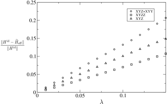
Figure 4.2: Here the ratio of the error terms to the ideal Hamiltonian $H^{\mathrm{id}}\equiv\frac{-k(-\lambda)^{k}}{(k-1)!}H^{\mathrm{comp}}$ is plotted. We examine three examples, a third order gadget simulating a single $XYZ$ interaction, a third order gadget simulating a pair of interactions $XYZ+XYY$, and a fourth order gadget simulating a fourth order interaction $XYZZ$. Here $\widetilde{H}_{\mathrm{eff}}$ is calculated by direct numerical computation without using perturbation theory. As expected the ratio of the norm of the error terms to $H^{\mathrm{id}}$ goes linearly to zero with shrinking $\lambda$.

4.5 Derivation of Perturbative Formulas

In this section we give a self-contained presentation of the derivations for the method of degenerate perturbation theory used in this paper. We closely follow Bloch[28]. Given a Hamiltonian of the form

$$H=H^{(0)}+\lambda V$$ (4.57)

we wish to find the effective Hamiltonian induced by the perturbation $\lambda V$ on the ground space of $H^{(0)}$. In what follows, we assume that the ground space of $H^{(0)}$ has energy zero. This simplifies notation, and the generalization to nonzero ground energy is straightforward. To further simplify notation we define

$$\hat{V}=\lambda V.$$ (4.58)

Suppose the ground space of $H^{(0)}$ is $d$-dimensional and denote it by $\mathcal{E}^{(0)}$. Let $\left|{\psi_{1}}\right\rangle,\ldots,\left|{\psi_{d}}\right\rangle$ be the perturbed eigenstates arising from the splitting of this degenerate ground space, and let $E_{1},\ldots,E_{d}$ be their energies. Furthermore, let $\left|{\alpha_{j}}\right\rangle=P_{0}\left|{\psi_{j}}\right\rangle$ where $P_{0}$ is the projector onto the unperturbed ground space of $H^{(0)}$. If $\lambda$ is sufficiently small, $\left|{\alpha_{1}}\right\rangle,\ldots,\left|{\alpha_{d}}\right\rangle$ are linearly independent, and we can define an operator $\mathcal{U}$ such that

$$\mathcal{U}\left|{\alpha_{j}}\right\rangle=\left|{\psi_{j}}\right\rangle$$ (4.59)

and

$$\mathcal{U}\left|{\phi}\right\rangle=0\quad\forall\left|{\phi}\right\rangle\in\mathcal{E}^{(0)\perp}.$$ (4.60)

Now let $\mathcal{A}$ be the operator

$$\mathcal{A}=P_{0}\hat{V}\mathcal{U}.$$ (4.61)

$\mathcal{A}$ has $\left|{\alpha_{1}}\right\rangle,\ldots,\left|{\alpha_{d}}\right\rangle$ as its eigenstates, and $E_{1},\ldots,E_{d}$ as its corresponding energies. To see this, note that since $H^{(0)}$ has zero ground state energy

$$P_{0}\hat{V}=P_{0}(H^{(0)}+\hat{V})=P_{0}H.$$ (4.62)

Thus,

$$\mathcal{A}\left|{\alpha_{j}}\right\rangle = P_{0}\hat{V}\mathcal{U}\left|{\alpha_{j}}\right\rangle$$ (4.63)

$$= P_{0}\hat{V}\left|{\psi_{j}}\right\rangle$$

$$= P_{0}H\left|{\psi_{j}}\right\rangle$$

$$= P_{0}E_{j}\left|{\psi_{j}}\right\rangle$$

$$= E_{j}\left|{\alpha_{j}}\right\rangle.$$

The essential task in this formulation of degenerate perturbation theory is to find a perturbative expansion for $\mathcal{U}$. From $\mathcal{U}$ one can obtain $\mathcal{A}$ by equation 4.61. By diagonalizing $\mathcal{A}$ one obtains $E_{1},\ldots,E_{d}$, and $\left|{\alpha_{1}}\right\rangle,\ldots,\left|{\alpha_{d}}\right\rangle$. Then, by applying $\mathcal{U}$ to $\left|{\alpha_{j}}\right\rangle$ one obtains $\left|{\psi_{j}}\right\rangle$. So, given a perturbative formula for $\mathcal{U}$, all quantities of interest can be calculated. Rather than diagonalizing $\mathcal{A}$ to obtain individual eigenstates and eigenenergies, one can instead compute an effective Hamiltonian for the entire perturbed eigenspace, defined by

$$H_{\mathrm{eff}}(H,d)\equiv\sum_{j=1}^{d}E_{j}\left|{\psi_{j}}\right\rangle\left\langle{\psi_{j}}\right|.$$ (4.64)

This is given by

$$H_{\mathrm{eff}}(H,d)=\mathcal{U}\mathcal{A}\mathcal{U}^{\dagger}.$$ (4.65)

To derive a perturbative formula for $\mathcal{U}$, we start with Schrödinger’s equation:

$$H\left|{\psi_{j}}\right\rangle=E_{j}\left|{\psi_{j}}\right\rangle.$$ (4.66)

By equation 4.62, left-multiplying this by $P_{0}$ yields

$$P_{0}\hat{V}\left|{\psi_{j}}\right\rangle=E_{j}\left|{\alpha_{j}}\right\rangle.$$ (4.67)

By equation 4.60,

$$\mathcal{U}P_{0}=\mathcal{U}.$$ (4.68)

Thus left-multiplying equation 4.67 by $\mathcal{U}$ yields

$$\mathcal{U}\hat{V}\left|{\psi_{j}}\right\rangle=E_{j}\left|{\psi_{j}}\right\rangle.$$ (4.69)

By subtracting 4.69 from 4.66 we obtain

$$(H-\mathcal{U}\hat{V})\left|{\psi_{j}}\right\rangle=0.$$ (4.70)

The span of $\left|{\psi_{j}}\right\rangle$ we call $\mathcal{E}$. For any state $\left|{\beta}\right\rangle$ in $\mathcal{E}$ we have

$$(H-\mathcal{U}\hat{V})\left|{\beta}\right\rangle=0.$$ (4.71)

Since $\mathcal{U}\left|{\gamma}\right\rangle\in\mathcal{E}$ for any state $\left|{\gamma}\right\rangle$, it follows that

$$(H-\mathcal{U}\hat{V})\mathcal{U}=0.$$ (4.72)

This equation can be rewritten as

$$H^{(0)}\mathcal{U}=-\hat{V}\mathcal{U}+\mathcal{U}\hat{V}\mathcal{U}.$$ (4.73)

Defining $Q_{0}=\mathds{1}-P_{0}$ we have

$$\mathcal{U}=P_{0}\mathcal{U}+Q_{0}\mathcal{U}.$$ (4.74)

Substituting this into the left side of 4.73 yields

$$H^{(0)}Q_{0}\mathcal{U}=-\hat{V}\mathcal{U}+\mathcal{U}\hat{V}\mathcal{U},$$ (4.75)

because $H^{(0)}P_{0}=0$. In $\mathcal{E}^{(0)\perp}$, $H^{(0)}$ has a well defined inverse and one can write

$$Q_{0}\mathcal{U}=-\frac{1}{H^{(0)}}Q_{0}(\hat{V}\mathcal{U}-\mathcal{U}\hat{V}\mathcal{U}).$$ (4.76)

Using equation 4.74, one obtains

$$\mathcal{U}=P_{0}\mathcal{U}-\frac{1}{H^{(0)}}Q_{0}(\hat{V}\mathcal{U}-\mathcal{U}\hat{V}\mathcal{U}).$$ (4.77)

By the definition of $\mathcal{U}$ it is apparent that $P_{0}\mathcal{U}=P_{0}$, thus this equation simplifies to

$$\mathcal{U}=P_{0}-\frac{1}{H^{(0)}}Q_{0}(\hat{V}\mathcal{U}-\mathcal{U}\hat{V}\mathcal{U}).$$ (4.78)

We now expand $\mathcal{U}$ in powers of $\lambda$ (equivalently, in powers of $\hat{V}$), and denote the $m^{\mathrm{th}}$ order term by $\mathcal{U}^{(m)}$. Substituting this expansion into equation 4.78 and equating terms at each order yields the following recurrence relations.

$$\mathcal{U}^{(0)} = P_{0}$$ (4.79)

$$\mathcal{U}^{(m)} = -\frac{1}{H^{(0)}}Q_{0}\left[\hat{V}\mathcal{U}^{(m-1)}-\sum_{p=1}^{m-1}\mathcal{U}^{(p)}\hat{V}\mathcal{U}^{(m-p-1)}\right]\quad(m=1,2,3\ldots)$$ (4.80)

Note that the sum over $p$ starts at $p=1$, not $p=0$. This is because

$$\frac{1}{H^{(0)}}Q_{0}\mathcal{U}^{(0)}=\frac{1}{H^{(0)}}Q_{0}P_{0}=0.$$ (4.81)

Let

$$S^{l}=\left\{\begin{array}[]{ll}\frac{1}{\left(-H^{(0)}\right)^{l}}Q_{0}&\textrm{if $l>0$}\\ -P_{0}&\textrm{if $l=0$}\end{array}\right..$$ (4.82)

$\mathcal{U}^{(m)}$ is of the form

$$\mathcal{U}^{(m)}={\sum}^{\prime}S^{l_{1}}\hat{V}S^{l_{2}}\hat{V}\ldots S^{l_{m}}\hat{V}P_{0},$$ (4.83)

where $\sum^{\prime}$ is a sum over some subset of $m$-tuples $(l_{1},l_{2},\ldots,l_{m})$ such that

$$l_{i}\geq 0\quad(i=1,2,\ldots,m)$$ (4.84)

$$l_{1}+l_{2}+\ldots+l_{m}=m.$$ (4.85)

The proof is an easy induction. $\mathcal{U}^{(0)}$ clearly satisfies this, and we can see that if $\mathcal{U}^{(j)}$ has these properties for all $j<m$, then by recurrence 4.80, $\mathcal{U}^{(m)}$ also has these properties.

All that remains is to prove that the subset of allowed $m$-tuples appearing in the sum $\sum^{\prime}$ are exactly those which satisfy

$$l_{1}+\ldots+l_{p}\geq p\quad(p=1,2,\ldots,m-1).$$ (4.86)

Following [28], we do this by introducing stairstep diagrams to represent the $m$-tuples, as shown in figure 4.3.

Figure 4.3: From a given $m$-tuple $(l_{1},l_{2},\ldots,l_{m})$ we construct a corresponding stairstep diagram by making the $j^{\mathrm{th}}$ step have height $l_{j}$, as illustrated above.

The $m$-tuples with property 4.86 correspond to diagrams in which the steps lie above the diagonal. Following [28] we call these convex diagrams. Thus our task is to prove that the sum $\sum^{\prime}$ is over all and only the convex diagrams. To do this, we consider the ways in which convex diagrams of order $m$ can be constructed from convex diagrams of lower order. We then relate this to the way $\mathcal{U}^{(m)}$ is obtained from lower order terms in the recurrence 4.80.

In any convex diagram, $l_{1}\geq 1$. We now consider the two cases $l_{1}=1$ and $l_{1}>1$. In the case that $l_{1}=1$, the diagram is as shown on the left in figure 4.4.

Figure 4.4: A convex diagram must have either $l_{1}=1$ or $l_{1}>1$. In either case, the diagram can be decomposed as a concatenation of lower order convex diagrams.

In any convex diagram of order $m$ with $l_{1}=1$, there is an intersection with the diagonal after one step, at the point that we have labelled $c$. The diagram from $c$ to $b$ is a convex diagram of order $m-1$. Conversely, given any convex diagram of order $m-1$ we can construct a convex diagram of order $m$ by adding one step to the beginning. Thus the convex diagrams of order $m$ with $l_{1}=1$ correspond bijectively to the convex diagrams of order $m-1$.

The case $l_{1}>1$ is shown in figure 4.4 on the right. Here we introduce the line from $a^{\prime}$ to $b^{\prime}$, which is parallel to the diagonal, but higher by one step. Since the diagram must end at $b$, it must cross back under $a^{\prime}b^{\prime}$ at some point. We’ll label the first point at which it does so as $c^{\prime}$. In general, $c^{\prime}$ can equal $b^{\prime}$. The curve going from $a^{\prime}$ to $c^{\prime}$ is a convex diagram of order $p$ with $1\leq p\leq m-1$, and the curve going from $c$ to $b$ is a convex diagram of order $n-p-1$ (which may be order zero if $c^{\prime}$ = $b^{\prime}$). Since $c^{\prime}$ exists and is unique, this establishes a bijection between the convex diagrams of order $m$ with $l_{1}>1$, and the set of the pairs of convex diagrams of orders $p$ and $n-p-1$, for $1\leq p\leq n-1$.

Examining the recurrence 4.80, we see that the $l_{1}=1$ diagrams are exactly those which arise from the term

$$\frac{Q_{0}}{H^{(0)}}\hat{V}\mathcal{U}^{(m-1)}$$ (4.87)

and the $l_{1}>1$ diagrams are exactly those which arise from the term

$$\frac{Q_{0}}{H^{(0)}}\sum_{p=1}^{m-1}\mathcal{U}^{(p)}\hat{V}\mathcal{U}^{(n-p-1)}.$$ (4.88)

which completes the proof that $\sum^{\prime}$ is over the $m$-tuples satisfying equation 4.86.

4.6 Convergence of Perturbation Series

Here we show that the perturbative expansion for $\mathcal{U}$ given in equation 4.27 converges for

$$\|\lambda V\|<\frac{\gamma}{4}.$$ (4.89)

By equation 4.20, the convergence of $\mathcal{U}$ also implies the convergence of $\mathcal{A}$. Applying the triangle inequality to equation 4.27 yields

$$\|\mathcal{U}\|\leq 1+\sum_{m=1}^{\infty}\|\mathcal{U}^{(m)}\|.$$ (4.90)

Substituting in equation 4.28 and applying the triangle inequality again yields

$$\|\mathcal{U}\|\leq 1+\sum_{m=1}^{\infty}\lambda^{m}\sum_{(m)}\|S^{l_{1}}\ldots VS^{l_{m}}VP_{0}\|.$$ (4.91)

By the submultiplicative property of the operator norm,

$$\|\mathcal{U}\|\leq 1+\sum_{m=1}^{\infty}\lambda^{m}\sum_{(m)}\|S^{l_{1}}\|\cdot\|V\|\ldots\|V\|\cdot\|S^{l_{m}}\|\cdot\|V\|\cdot\|P_{0}\|.$$ (4.92)

$\|P_{0}\|=1$, and by equation 4.22 we have

$$\|S^{l}\|=\frac{1}{(E_{1}^{(0)})^{l}}=\frac{1}{\gamma^{l}}.$$ (4.93)

Since the sum in equation 4.92 is over $l_{1}+\ldots+l_{m}=m$, we have

$$\|\mathcal{U}\|\leq 1+\sum_{m=1}^{\infty}\sum_{(m)}\frac{\|\lambda V\|^{m}}{\gamma^{m}}.$$ (4.94)

The sum $\sum_{(m)}$ is over a subset of the $m$-tuples adding up to $m$. Thus, the number of terms in this sum is less than the number of ways of obtaining $m$ as a sum of $m$ nonnegative integers. By elementary combinatorics, the number of ways to obtain $n$ as a sum of $r$ nonnegative integers is $\binom{n+r-1}{n}$, thus

$$\|\mathcal{U}\|\leq 1+\sum_{m=1}^{\infty}\binom{2m-1}{m}\frac{\|\lambda V\|^{m}}{\gamma^{m}}.$$ (4.95)

Since

$$\sum_{j=0}^{2m-3}\binom{2m-1}{j}=2^{2m-1},$$ (4.96)

we have

$$\binom{2m-1}{m}\leq 2^{2m-1}.$$ (4.97)

Substituting this into equation 4.95 converts it into a convenient geometric series:

$$\|\mathcal{U}\|\leq 1+\sum_{m=1}^{\infty}2^{2m-1}\frac{\|\lambda V\|^{m}}{\gamma^{m}}.$$ (4.98)

This series converges for

$$\frac{4\|\lambda V\|}{\gamma}<1.$$ (4.99)

Chapter 5 Multiplicity and Unity

The fox knows many things but the hedgehog knows one big thing.
-Archilochus

In his essay “The Hedgehog and the Fox,” Isaiah Berlin, echoing Archilochus, classified thinkers into two categories, hedgehogs, who look for unity and generality, and foxes, who revel in the variety and complexity of the universe. In this chapter I will revisit the content of my thesis from each of these points of view.

5.1 Multiplicity

…you shall not add to the misery and sorrow of the world, but shall smile to the infinite variety and mystery of it.
-Sir William Saroyan

In this thesis I have spoken about many models of computation, especially the adiabatic, topological, and circuit models. Each of these models of computation can solve exactly the same set of problems in polynomial time. Thus one might ask: “why bother”? Why not just stick to the quantum circuit model?

As the many examples in this thesis have shown, sticking to only one model of quantum computation would be a mistake. The most obvious justification for considering alternative models of quantum computation is that they provide promising alternatives for the physical implementation of quantum computers. As discussed in chapters 1 and 2, the main barrier to practical quantum computation is the effect of noise. Three types of quantum computer show promise for overcoming this barrier: quantum circuits, by means of active error correction, adiabatic quantum computers, by their inherent indifference to local properties, and topological quantum computers by their energy gap, as discussed in chapter 2. It is not yet clear which of these strategies will prove most useful, and this provides justification for investigating all of them.

A skeptic might protest that this only justifies investigation of physically realistic models of quantum computation. Some of the models discussed in the literature, and in this thesis, are not very physically realistic. For example, it seems unlikely that adiabatic computation with 4-local Hamiltonians, or quantum walks on exponentially many nodes will be implemented in laboratories. However, even models slightly removed from physical practicality have proven useful in the development of practical physical implementations. For example, we now know that adiabatic quantum computation with 2-local Hamiltonians is universal. This was originally proven by showing that 5-local Hamiltonians are computationally universal, and then making a series of reductions from 3-local down to 2-local. Even now, the best known direct universality proof is for 3-local adiabiatic quantum computation[133].

There is a second, less obvious justification for considering multiple models of quantum computation. Although all of quantum algorithms could in principle be formulated using the quantum circuit model, this is not how quantum computation actually developed. The quantum algorithms for factoring and searching were discovered using the quantum circuit model. The quantum speedups for NAND tree evaluation and simulated annealing were discovered using quantum walks. The quantum algorithm for approximating Jones polynomials was discovered using topological quantum computation. History has shown us that a particular model of quantum computation gives us a perspective from which certain quantum algorithms are easily visible, while they remain obscure from the perspective of other models.

Having argued the virtues of having a multiplicity of models of quantum computation, the time has come to put this principle into action. That is, I will propose a direction for further research based on the premise that formulating additional models of quantum computation is useful even if the models are not directly practical.

One striking thing about the topological model of quantum computation is its indifference to the details of the manipulations of the particles. Only the topology of the braiding matters, and the specific geometry is irrelevant. Let’s now push this a step further and consider a model where even the topology is irrelevant, and the only thing that matters is how the particles were permuted. Just as the braiding of anyons induces a representation of the braid group, we analogously expect that the permutation of the particles induces a representation of the symmetric group.

Such a model is not entirely without physical motivation. The exchange statistics of Bosons and Fermions are exactly the two one-dimensional representations of the symmetric group. Particles with exchange statistics given by a higher dimensional representation of the symmetric group have been proposed in the past. This is called parastatistics. Such particles have never been observed. However, based on the presently understood physics, they remain an exotic, but not inconcievable possibility[142]. Furthermore, many Hamiltonians in nature are symmetric under permutation of the particles. If a Hamiltonian has symmetry group $G$, then its degenerate eigenspaces will transform as representations of $G$, and these representations will generically be irreducible[91].

More precisely, suppose a Hamiltonian $H$ on $n$ particles has a $d$-fold degenerate eigenspace spanned by $\phi_{1}(x_{1},\ldots,x_{n}),\ldots,\phi_{d}(x_{1},\ldots,x_{n})$. We start with a given state within that space

$$\psi(x_{1},\ldots,x_{n})=\sum_{j=1}^{d}\alpha_{j}\phi_{j}(x_{1},\ldots,x_{n})$$

Then, if we permute the particles according to some permutation $\pi$ we obtain some other state $\psi(x_{\pi(1)},\ldots,x_{\pi(n)})$. Because the Hamiltonian is permutation symmetric, this state will lie within the same eigenspace. That is, there are some coefficients $\beta_{1},\ldots,\beta_{d}$ such that

$$\psi(x_{\pi(1)},\ldots,x_{\pi(n)})=\sum_{j=1}^{d}\beta_{j}\phi_{j}(x_{1},\ldots,x_{n}).$$

It is clear that the dependence of $\beta_{1},\ldots,\beta_{d}$ on $\alpha_{1},\ldots,\alpha_{d}$ is linear. Thus there is some matrix $M^{\pi}$ corresponding to permutation $\pi$:

$$\beta_{i}=\sum_{j=1}^{d}M^{\pi}_{ij}\alpha_{j}.$$

It is not hard to see that the mapping from permutations to their corresponding matrices is a group homomorphism. That is, these $d\times d$ matrices form a representation of the symmetric group $S_{n}$. If the $H$ has no other symmetries, then this representation will generically be irreducible[91].

As advocated above, I will not worry too much about the physical justification for the model, but instead consider just two questions. First, does the model lend itself to the the rapid solution of any interesting computational problems, and second, can it be efficiently simulated by quantum circuits? If both answers are yes, then we obtain new quantum algorithms.

The question of what problem this model of computation lends itself to has an obvious answer: the computation of representations of the symmetric group. There are many good reasons to restrict our consideration to only the irreducible representations. Any finite group has only finitely many irreducible representations but infinitely many reducible representations. These reducible representations are always the direct sum of multiple irreducible representations. Thus, by performing a computation with a reducible representation we would merely be performing a superposition of computations with irreducible representations.

In chapter 3 we saw that if we can apply a representation of the braid group then, using the Hadamard test, we can estimate the matrix elements of this representation to polynomial precision. Furthermore, by sampling over the diagonal matrix elements we can estimate the normalized trace of the representation to polynomial precision. If we instead have a representation of the symmetric group, the situation is precisely analogous. The trace of a group representation is called its character. Characters of group representations have many uses not only in mathematics, but also in physics and chemistry. Note that, unlike the matrix elements of a representation, its character is basis independent.

Just as with anyonic quantum computation, we can imagine the particles initially positioned along a line. We then allow ourselves to swap neighbors. The runtime of an algorithm is the number of necessary swaps. Interestingly, in the parastistical model of computation, no algorithm has runtime more than $O(n^{2})$, because there are only finitely many permutations and each of them can be constructed using at most $O(n^{2})$ swaps.

To formulate the concrete computational problems we’ll need to delve a little bit into the specifics of the irreducible representations of the symmetric group. The irreducible representations of $S_{n}$ are indexed by the Young diagrams of $n$ boxes. These are all the possible partitions of the $n$ boxes into rows, where the rows are arranged in descending order of length. The example $n=4$ is shown in figure 5.1. The matrix elements of these representations depend on a choice of basis. For our purposes it is essential that the basis be chosen so that the representation is unitary. The most widely used such basis is called the Young-Yamanouchi basis[91]. In this basis the irreducible representations are sparse orthogonal matricees. For the irreducible representation corresponding to a Young diagram $\lambda$, the Young-Yamanouchi basis vectors correspond to the set of standard Young tableaux compatible with lambda. These are all the numberings of boxes so that if we added the boxes in this order, the configuration would be a valid Young diagram after every step. This is illustrated in figure 5.2. It is not hard to see that for some $\lambda$, the number of standard tableaux, and hence the dimension of the representation, is exponential in $n$.

Figure 5.1: The Young diagrams with four boxes. They correspond to the irreducible representations of $S_{4}$.

Figure 5.2: Above we show an example Young tableau, and beneath it the corresponding sequence of Young diagrams from left to right.

Thus we can state the following computational problems regarding $S_{n}$, which are solvable in $\mathrm{poly}(n)$ time in the parastatistical model of computation.

Problem: Calculate an irreducible representation for the symmetric group $S_{n}$. Input: A Young diagram specifying the irreducible representation, a permutation from $S_{n}$, a pair of standard Young tableaux indicating the desired matrix element, and a polynomially small parameter $\epsilon$. Output: The specified matrix element to within $\pm\epsilon$. Problem: Calculate a character for the symmetric group $S_{n}$. Input: A Young diagram $\lambda$ specifying the irreducible representation, a permutation $\pi$ from $S_{n}$, and a polynomially small parameter $\epsilon$. Output: Let $\chi_{\lambda}(\pi)$ be the character, and let $d_{\lambda}$ be the dimension of the irreducible representation. The output is $\chi_{\lambda}(\pi)/d_{\lambda}$ to within $\pm\epsilon$. Next, we must find out how hard these problems are classically. If classical polynomial time algorithms for these problems are known then we have not discovered anything interesting. Without looking into the classical computation literature there are already two things we can say. First, as noted above, for some Young diagrams of $S_{n}$, the corresponding representation has dimension exponential in $n$. Thus the above problems cannot be solved classically in polynomial time by directly using matrix multiplication. Second, the irreducible representations have both positive and negative matrix elements in all of the bases discussed in standard references[91, 29]. Thus interference effects are important, so naive Markov chain methods will not work.

To go beyond these simple observations, we must consult the relevant experts and body of literature. As shown in [95], the problem of exactly evaluating the characters of the irreducible representations of the symmetric group is #P-complete. This rules out the possibility that some ingenious closed form expression for the characters is buried in the math literature somewhere. The characters are obtained in the parastatistical model of computation to only polynomial precision. This corresponds to the precision one could obtain by classically sampling from the diagonal matrix elements of the representation. Thus, the most likely scenario by which these algorithms could fail to be interesting is if the individual matrix element of the irreducible representations of the symmetric group are easy to compute classically, and the only reason that computing the characters is hard is that there are exponentially many of these matrix elements to add up. However, the sources I have consulted do not provide any way to obtain matrix elements of the irreducible representations of the $S_{n}$ in $\mathrm{poly}(n)$ time for arbitrary permutations[129, 91, 29]. Furthermore, there is a body of work on how to improve the efficiency of exponential time algorithms for this problem[175, 176, 64, 49]. Unless this entire body of work is misguided, no polynomial-time methods for computing such matrix elements were known when these papers were written.

A completeness result would provide even stronger evidence of the difficulty of these problems. The problems of estimating Jones polynomials discussed in section 3 were each BQP or DQC1 complete. In general one could conjecture that for any representation dense in a unitary group of exponentially large dimension, the problem of estimating matrix elements to polynomial precision is BQP-complete and the problem of estimationg normalized characters to polynomial precision is DQC1-complete. However, because the symmetric group is finite, no representation of it can be dense in a continuous group. Thus it seems unlikely that the problems of estimating the matrix elements and characters of the symmetric group are BQP-complete or DQC1-complete. Furthermore, the fact that no parastatistical algorithm on $n$ particles requires more than $O(n^{2})$ computational steps makes it seem unlikely that this model is universal.

Next we must see whether the parastatistical model of computation can be simulated in polynomial time by standard quantum computers. If so we obtain two new polynomial time quantum algorithms apparently providing exponential speedup over known classical algorithms. Normally the search for quantum algorithms is a pursuit fraught with frustration. However, in this case we have a win-win situation. If the parastatistical model cannot be simulated by quantum computers in polynomial time, then instead of quantum algorithms we have a physically plausible model of computation not contained in BQP, which is also very exciting.

A detailed examination of the Young-Yamanouchi matrices in [91] makes me fairly convinced that the parastatistical model of computation can be simulated in polynomial time by quantum circuits. Specifically, it appears that this can be done very analogously to the implementation of the Fibonacci representation of the braid group in chapter 3. However, this is not the place to discuss such details. Instead I will now switch teams, and take the side of the hedgehog.

5.2 Unity

…the world will somehow come clearer and we will grasp the true strangeness of the universe. And the strangeness will all prove to be connected and make sense.
-E.O. Wilson

Upon examining the catalogue of quantum algorithms in chapter 1, a striking pattern emerges. Although the quantum algorithms are superficially widely varied, the exponential speedups for non-oracular problems generally fall into two broad families: the speedups obtained by reduction to hidden subgroup problems, and the speedups related to knot invariants. Interestingly, both of these families of speedups rely on representation theory. The speedups for the hidden subgroup related problems are based on the Fourier transform over groups. Such a Fourier transform goes between the computational basis, and a basis made from matrix elements of irreducible representations. The speedups for the evaluation of knot invariants are based on implementating a unitary representation of the braid group using quantum circuits. It is therefore tempting to look for some grand unification to unite all exponential speedups into one representation-theoretic framework.

I do not know whether such a grand unification is possible, nevermind how to carry it out. However, I will offer a bold speculation as to a possible route forward. Rather than starting with the Fourier transform, lets first consider the Schur transform. Like the Fourier transform, the Schur transform can be efficiently implented using quantum circuits [92], and has applications in quantum information processing. Furthermore, it has a more obvious connection to multiparticle physics than does the Fourier transform. For example, suppose we have two spin-1/2 particles. The Hilbert space of quantum states for these spins is four dimensional. One basis we can choose for this Hilbert space is obtained by taking the tensor product of $\sigma_{z}$-basis for each spin:

$$\begin{array}[]{l}\left|{\uparrow}\right\rangle\left|{\uparrow}\right\rangle\\ \left|{\uparrow}\right\rangle\left|{\downarrow}\right\rangle\\ \left|{\downarrow}\right\rangle\left|{\uparrow}\right\rangle\\ \left|{\downarrow}\right\rangle\left|{\downarrow}\right\rangle\end{array}$$

Another basis can be obtained as the simultaneous eigenbasis of the total angular momentum $\sigma_{x}^{(1)}\sigma_{x}^{(2)}+\sigma_{y}^{(1)}\sigma_{y}^{(2)}+\sigma_{z}^{(1)}\sigma_{z}^{(2)}$ and the total azimuthal angular momentum $\sigma_{z}^{(1)}+\sigma_{z}^{(2)}$. This basis is

$$\begin{array}[]{l}\left|{\uparrow}\right\rangle\left|{\uparrow}\right\rangle\\ \frac{1}{\sqrt{2}}\left(\left|{\uparrow}\right\rangle\left|{\downarrow}\right\rangle+\left|{\downarrow}\right\rangle\left|{\uparrow}\right\rangle\right)\\ \left|{\downarrow}\right\rangle\left|{\downarrow}\right\rangle\\ \frac{1}{\sqrt{2}}\left(\left|{\uparrow}\right\rangle\left|{\downarrow}\right\rangle+\left|{\downarrow}\right\rangle\left|{\uparrow}\right\rangle\right)\end{array}$$

The Schur transform in this case is just the unitary change of basis between these two bases. The general case is explained in [92], and is fairly analogous.

The matrix elements appearing in this change of basis are known as Clebsch-Gordon coefficients, and are tabulated in most undergraduate quantum mechanics textbooks. According to [136], the coefficients appearing in the fusion rules of a topological quantum field theory are essentially a generalization of Clebsch-Gordon coefficients. Thus, I offer the conjecture that one could implement the Schur transform directly using the fusion rules of some TQFT. (Since some TQFTs are universal for quantum computation, and Schur transforms can be efficiently computed, one could always take the circuit for finding Schur transforms and convert it into some extremely complicated braiding of anyons. This is not what we are looking for.)

The Schur transform is related to the Fourier transform over the symmetric group[92]. Thus, if a direct TQFT implementation of the Schur transform were found then one could next look for a direct anyonic implementations of Fourier transforms. I therefore propose the conjecture that the two classes of quantum algorithms correspond to the two components of a topological quantum field theory: the knot invariant algorithms correspond to the braiding rules, and the hidden subgroup problems correspond to the fusion rules.

Appendix A Classical Circuit Universality

Consider an arbitrary function $f$ from $n$ bits to one bit. $f$ can be specified by listing each bitstrings $x\in\{0,1\}^{n}$ such that $f(x)=1$. To show the universality of the $\{\mathrm{AND,NOT,OR,FANOUT}\}$ gate set, we wish to construct a circuit out of these gates that implements $f$. We’ll diagrammatically represent these gates using

From two-input AND gates we can construct an $m$-input AND gate for any $m$. The example $m=4$ is shown below.

An $m$-input OR gate can be constructed from 2-input OR gates, and an $m$-output FANOUT gate can be constructed from 2-output FANOUT gates similarly. The $m$-input AND gate accepts only the string $111\ldots$. To accept a different string, one can simply attach NOT gates to all the inputs which should be 0. Using AND and NOT gates, one can thus make a circuit to accept each bitstring accepted by $f$. These can then be joined together using a multi-input OR circuit. FANOUT gates are used to supply the inputs to each of these. The resulting circuit simulates $f$ as shown in figure A.1.

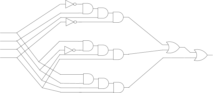
Figure A.1: The Boolean circuit with four bits of input and one bit of output which accepts only the inputs $0110$, $1011$, and $1111$ is implemented by the shown circuit. Any Boolean function can be implemented similarly, as described in the text.

To implement a function with multiple bits of output, one can consider each bit of output to be a separate single-bit Boolean function of the inputs, and construct a circuit for each bit of output accordingly.

Appendix B Optical Computing

Quantum mechanics bears a close resemblance to classical optics. An optical wave associates an amplitude with each point in space. A quantum wavefunction associates an amplitude with each possible configuration of the system. Whereas an optical wave is a function of at most three spatial variables, a quantum wavefunction of a system of particles is a function of all the parameters needed to describe the configuration of the particles. Thus classical optics lacks the exponentially high-dimensional state space of quantum mechanics. The similarity between classical optics and quantum mechanics is of course no coincidence, as photons are governed by quantum mechanics. Essentially, classical optics treats the case where these photons are independent and unentangled, so that the intensity of light on at a given point on the detector is simply proportional to the probability density for a single photon to be detected at that point if it were sent through the optical apparatus by itself.

Figure B.1: A collimated beam shined at an angle toward a lens will have phases varying linearly across the face of the lens, due to the extra distance that some rays must travel. Such a beam gets focused to a point on the focal plane whose location depends on the angle at which the beam was shined onto the lens. Thus, the amplitude across the lens of $e^{ikx}$ gets transformed to an amplitude across the focal plane of $\delta(x+k)$. Since a lens is a linear optical device, any superposition of plane waves will be mapped to the corresponding superposition of delta functions. Thus the amplitude across the focal plane will be the Fourier transform of the amplitude across the face of the lens.

Fourier transforms are an important primitive in quantum computing, and lie at the heart of the factoring algorithm, and several other quantum algorithms. As shown in [160], quantum computers can perform Fourier transforms on $n$-qubits using $O(n^{3})$ gates. Consider the computational basis states of $n$-qubits as corresponding to the numbers $\{0,1,\ldots,2^{n}-1\}$ via place value. The quantum Fourier transform on $n$ qubits is the following unitary transformation.

$$U_{F}\sum_{x=0}^{2^{n}-1}a(x)\left|{x}\right\rangle=\frac{1}{\sqrt{2^{n}}}\sum_{k=0}^{2^{n}-1}\sum_{x=0}^{2^{n}-1}e^{i2\pi xk/2^{n}}a(x)\left|{k}\right\rangle.$$

The Fourier can be performed optically with a single lens, as shown in figure B.1. Before digital computers became as powerful as they are today, people used to develop optical schemes for analog computation. Many of them were based in some way on the optical Fourier transform.

Another important primitive in quantum algorithms is phase kickback. Typically, an oracle $U_{f}$ for a give function $f$ acts according to

$$U_{f}\left|{x}\right\rangle\left|{y}\right\rangle=\left|{x}\right\rangle\left|{(y+f(x))\ \mathrm{mod}\ 2^{n_{o}}}\right\rangle,$$

where $n_{o}$ is the number of output bits. Normally, one chooses $y=0$ so that the output register contains $f(x)$ after applying the oracle. However, if one instead prepares the output register in the state

$$\left|{\psi}\right\rangle=\frac{1}{\sqrt{2^{n_{o}}}}\sum_{y=0}^{2^{n_{o}}}e^{i2\pi y/2^{n_{o}}}\left|{y}\right\rangle,$$

$f(x)$ will be written into the phase instead of the qubits:

$$U_{f}\left|{x}\right\rangle\left|{\psi}\right\rangle=e^{i2\pi f(x)/2^{n_{o}}}\left|{x}\right\rangle\left|{\psi}\right\rangle.$$

This is because, for the process of adding $z$ modulo $2^{n_{o}}$, $\left|{\psi}\right\rangle$ is an eigenstate with eigenvalue $e^{i2\pi z/2^{n_{o}}}$.

Phase kickback also has an optical analogue. Simply constuct a sheet of glass whose thickness is proportional to $f(x)$. Because light travels more slowly through glass than through air, the beam experiences a phase lag proportional to the thickness of glass it passes through. Now consider the following optical “algorithm”. For simplicity we’ll demonstrate it in two dimensions, althogh it could also be done in three. We are given a piece of glass whose thickness is given by a smooth function $f(x)$. Because it is smooth, $f(x)$ is locally linear, and so the sheet looks locally like a prism. By inserting this glass between two lenses, as shown in figure B.2, we can determine the angle of this prism (i.e. $\frac{df}{dx}$) by the location of the spot made on the detector.

Figure B.2: At the left, a point source produces light. This is focused into a collimated beam by a lens. The beam then passes through a glass sheet which deflects the beam. The second lens then focuses the beam to a point on the detector whose location depends on the thickness gradient of the glass sheet.

By the analogies discussed above, this has an alternative description in terms of Fourier transforms, and an analogous quantum algorithm, as shown in figure B.3.

Figure B.3: Intially one starts with a given basis state. This is then Fourier transformed to yield the uniform superposition. A phase shift proportional to $f(x)$ is then performed. If $f(x)$ is locally linear than, the resulting shifted state is a plane wave $e^{if^{\prime}(x)x}$. The second Fourier transform then converts this to a basis state $\left|{f^{\prime}(x)}\right\rangle$.

So far, this is an unimpressive accomplishment. Both determining the angle of a prism and approximating the derivative of an oracular function of one variable are easy tasks. Now recall the difference between optical and quantum computing. Namely, the quantum analogue can be extended to an arbitrary number of dimensions. In particular, a phase proportional to $f(\vec{x})$ can easily be obtained using phase kickback, and a $d$-dimensional quantum Fourier transform can be achieved by applying a quantum Fourier transform to each vector component. As a result, on a quantum computer, one can obtain the gradient of a function of $d$ variables by generalizing the above algorithm. This requires only a single query to the oracle to do the phase kickback. In contrast, classically estimating the gradient of an oracular function requires at least $d+1$ queries. This is described in [107].

A literature exists on analog optical computation. It might be interesting to investigate whether some existing optical algorithms have more powerful quantum analogues. Also, it seems that quantum computers would be naturally suited to the simulation of classical optics problems. Perhaps a quantum speedup could be obtained for optical problems of practical interest, such as ray tracing.

Appendix C Phase Estimation

Phase estimation for unitary operators was introduced in [115], and is explained nicely in [137]. Here I will describe this method, and discuss how it can be used to measure in the eigenbasis of physical observables.

Suppose you have a quantum circuit of $\mathrm{poly}(n)$ gates on $n$ qubits which implements the unitary transformation $U$. Suppose also you are given some eigenstate $\left|{\psi_{j}}\right\rangle$ of $U$. You can always efficiently estimate the corresponding eigenvalue to polynomial precision using phase estimation. The first step in constructing the phase estimation circuit is to construct a circuit for controlled-$U$.

Given an polynomial size quantum circuit for $U$, one can always construct a polynomial size quantum circuit for controlled-$U$, which is a unitary $\widetilde{U}$ on $n+1$ qubits defined by

$$\widetilde{U}\left|{0}\right\rangle\left|{\psi}\right\rangle = \left|{0}\right\rangle\left|{\psi}\right\rangle$$

$$\widetilde{U}\left|{1}\right\rangle\left|{\psi}\right\rangle = \left|{1}\right\rangle U\left|{\psi}\right\rangle$$

for any $n$-qubit state $\left|{\psi}\right\rangle$. One can do this by taking the quantum circuit for $U$ and replacing each gate with the corresponding controlled gate. Each gate in the original circuit acts on at most $k$ qubits, where $k$ is some constant independent of $n$. Then, the corresponding controlled gate acts on $k+1$ qubits. By general gate universality results, any unitary on a constant number of qubits can be efficiently implemented.

The phase estimation algorithm uses a series of controlled-$U^{2^{m}}$ operators for successive values of $m$. Given a quantum circuit for $U$, one can construct a quantum circuit for $U^{k}$ by concatenating $k$ copies of the original circuit. The resulting circuit for $U^{k}$ can then be converted into a circuit for controlled-$U^{k}$ as described above.

Now consider the following circuit, which performs phase estimation to three bits of precision.

The top three qubits collectively form the control register. The bottom $n$ qubits are initialized to the eigenstate $\left|{\psi_{j}}\right\rangle$ and form the target register. The initial array of Hadamard gates puts the control register into the uniform superposition. Thus the state of the $n+3$ qubits after this step is

$$\frac{1}{\sqrt{8}}\sum_{x=0}^{7}\left|{x}\right\rangle\left|{\psi_{j}}\right\rangle.$$

Here we are using place value to make a correspondence between the strings of 3 bits and the integers from 0 to 7. The contolled-$U^{2^{m}}$ circuits then transform the state to

$$\frac{1}{\sqrt{8}}\sum_{x=0}^{7}\left|{x}\right\rangle U^{x}\left|{\psi_{j}}\right\rangle.$$

$\left|{\psi_{j}}\right\rangle$ is an eigenstate of $U$, thus this is equal to

$$\frac{1}{\sqrt{8}}\sum_{x=0}^{7}\left|{x}\right\rangle e^{ix\theta_{j}}\left|{\psi_{j}}\right\rangle$$

where $e^{i\theta_{j}}$ is the eigenvalue of $\left|{\psi_{j}}\right\rangle$. Notice that the control register is not entangled with the target register. Performing an inverse Fourier transform on the control register thus yields

$$\left|{\lceil\frac{8}{2\pi}\theta_{j}\rfloor}\right\rangle,$$

where the notation $\lceil\cdot\rfloor$ indicates rounding to the nearest integer. Thus we obtain $\theta$ with three bits of precision.

Similarly, with $b$ qubits in the control register, one can obtain $\theta_{j}$ to $b$ bits of precision. The necessary Hadamard and Fourier transforms require only $\mathrm{poly}(b)$ gates to perform. However, in order to obtain $b$ bits of precision, one must have a circuit for controlled-$U^{2^{b}}$. The only known completely general way to construct a circuit for $U^{2^{b}}$ from a circuit for $U$ is to concatenate $2^{b}$ copies of the circuit for $U$. Thus, the total size of the circuit for phase estimation will be on the order of $2^{b}g+\mathrm{poly}(b)$, where $g$ is the number of gates in the circuit for $U$. Thus, $\theta_{j}$ is obtained by the phase estimation algorithm to within $\pm 2^{-b}$, and the dominant contribution to the total runtime is proportional to $2^{b}$. In other words, $1/\mathrm{poly}(n)$ precision can be obtained in $\mathrm{poly}(n)$ time.

For some special $U$, it is possible to construct a circuit for $U^{2^{b}}$ using $\mathrm{poly}(b)$ gates. For example, this is true for the operation of modular exponentiation. The quantum algorithm for factoring can be formulated in terms of phase estimation of the modular exponentiation operator, as described in chapter five of [137].

The phase estimation algorithm can be thought of as a special type of measurement. Suppose you are given a superposition of eigenstates of $U$. By linearity, the phase estimation circuit will perform the following transformation

$$\left|{00\ldots}\right\rangle\sum_{j}a_{j}\left|{\psi_{j}}\right\rangle\to\sum_{j}a_{j}\left|{\lceil\frac{8}{2\pi}\theta_{j}\rfloor}\right\rangle\left|{\psi_{j}}\right\rangle.$$

By measuring the control register in the computational basis, one obtains the result $\lceil\frac{8}{2\pi}\theta_{j}\rfloor$ with probability $|a_{j}|^{2}$. If the eigenvalues of $U$ are separated by at least $2^{-b}$, then one has thus performed a measurement in the eigenbasis of $U$.

Often, one is interested in measuring in the eigenbasis of some observable defined by a Hermition operator. For example, one may wish to measure in the eigenbasis of a Hamiltonian, or an angular momentum operator. This can be done by combining the techniques of phase estimation and quantum simulation. As discussed in section 1.3, it is generally believed that any physically realistic observable can be efficiently simulated using a quantum circuit. More precisely, for any observable $H$, one can construct a circuit for $U=e^{iHt}$, where the number of gates is polynomial in $t$. Using this $U$ in the phase estimation algorithm, one can measure eigenvalues of $H$ to polynomial precision.

Appendix D Minimizing Quadratic Forms

A quadratic form is a function of the form $f(x)=x^{T}Mx+b\cdot x+c$, where $M$ is a $d\times d$ matrix, $x$ and $b$ are $d$-dimensional vectors, and $c$ is a scalar. Here we consider $M$, $x$, $b$, and $c$ to be real. Without loss generality we may assume that $M$ is symmetric. If $M$ is also positive definite, then $f$ has a unique minimum. In addition to its intrinsic interest, the problem of finding this minimum by making queries to a blackbox for $f$ can serve as an idealized mathematical model for numerical optimization problems.

Andrew Yao proved in 1975 that $\Omega(d^{2})$ classical queries are necessary to find the minimum of a quadratic form[177]. In 2004, I found that a single quantum query suffices to estimate the gradient of a blackbox function, whereas a minimum of $d+1$ queries are required classically[107]. One natural application for this is gradient based numerical optimization. In 2005, David Bulger applied quantum gradient estimation along with Grover search to the problem of numerically finding the minimum to an objective function with many basin-like local minima[36]. In the same paper he suggested that it would be interesting to analyze the speedup obtainable by applying quantum gradient estimation to the problem of minimizing a quadratic form. In this appendix, I show that a simple quantum algorithm based on gradient estimation can find the minimum of a quadratic form using only $O(d)$ queries, thus beating the classical lower bound.

For the blackbox for $f$ to be implemented on a digital computer, its inputs and outputs must be discretized, and represented with some finite number of bits. For present purposes, we shall ignore the “numerical noise” introduced by this discretization. In addition, on quantum computers, blackboxes must be implemented as unitary transformations. The standard way to achieve this is to let the unitary transformation $U_{f}\left|{x}\right\rangle\left|{y}\right\rangle=\left|{x}\right\rangle\left|{(y+f(x))\ \mathrm{mod}\ N_{o}}\right\rangle$ serve as the blackbox for $f$. Here $\left|{x}\right\rangle$ is the input register, $\left|{y}\right\rangle$ is the output register, and $N_{o}$ is the allowed range of $y$. By choosing $y=0$, one obtains $f(x)$ in the output register. As discussed in appendix B, by choosing

$$\left|{y}\right\rangle\propto\sum_{z}e^{-iz}\left|{z}\right\rangle,$$

one obtains $U_{f}\left|{x}\right\rangle\left|{y}\right\rangle=e^{if(x)}\left|{x}\right\rangle\left|{y}\right\rangle$, since, in this case, $\left|{y}\right\rangle$ is an eigenstate of addition modulo $N_{o}$. This is a standard technique in quantum computation, known as phase kickback.

There are a number of methods by which one can find the minimum of a quadratic form using $O(d)$ applications of quantum gradient estimation. Since each gradient estimation requires only a single quantum query to the blackbox, such methods only use $O(d)$ queries. One such method is as follows. First, we evaluate $\nabla f$ at $x=0$. If $M$ is symmetric, $\nabla f=2Mx+b$. Thus, this first gradient evaluation gives us $b$. Next we evaluate $\nabla f$ at $x=(1/2,0,0,\ldots)^{T}$. This yields $2M(1/2,0,0,\ldots)^{T}+b$. After subtracting $b$ we obtain the first column of $M$. Similarly, we then evaluate $\nabla f$ at $(0,1/2,0,0,\ldots)^{T}$ and subtract $b$ to obtain the second column of $M$, and so on, until we have full knowledge of $M$. Next we just compute $-\frac{1}{2}M^{-1}b$ to find the minimum of $f$. This process uses a total of $d+1$ gradient estimations, and hence $d+1$ quantum queries to the blackbox for $f$. Note that $M$ is always invertible since by assumption it is symmetric and positive definite.

Appendix E Principle of Deferred Measurement

The principle of deferred measurement is a simple but conceptually important fact which follows directly from the postulates of quantum mechanics[137]. It says:

Any measurement performed in the course of a quantum computation can always be deferred until the end of the computation. If any operations are conditionally performed depending on the measurement outcome they can be replaced by coherent conditional operations.

For example, consider a process on two qubits, where one qubit is measured in the computational basis, and if it is found to be in the state $\left|{1}\right\rangle$ then the second qubit is flipped.

By the principle of deferred measurement, this is exactly equivalent to

The principle of deferred measurement allows us to immediately see that the measurement based model of quantum computation (as described in section 1.6.5) can be efficiently simulated by quantum circuits. In addition, the principle of deferred measurement implies that uniform families of quantum circuits generated in polynomial time by quantum computers are no more powerful than uniform families of quantum circuits generated in polynomial time by classical computers, as shown below.

A quantum circuit can be described by series of bits corresponding to possible quantum gates. If a bit is 1 then the corresponding gate is present in the quantum circuit. Otherwise it is absent. Any quantum circuit on $n$ bits with $\mathrm{poly}(n)$ gates chosen from a finite set can be described by $\mathrm{poly}(n)$ classical bits in this way. We can think of the quantum circuit as a series of classically controlled gates, one for each bit in the description. Now suppose these bits are generated by a quantum computer, which I’ll call the control circuit. By the principle of deferred measurement, these classically controlled gates can be replaced by quantum controlled gates. We now consider the control circuit and these controlled gates together as one big quantum circuit. It is still of polynomial size, and it is controlled by the classical computer that generated the control circuit. Thus it is in BQP.

Appendix F Adiabatic Theorem

F.1 Main Proof

This appendix give a proof of the adiabatic theorem due to Jeffrey Goldstone [81].

Theorem 5.

Let $H(s)$ be a finite-dimensional twice differentiable Hamiltonian on $0\leq s\leq 1$ with a nondegenerate ground state $\left|{\phi_{0}(s)}\right\rangle$ separated by an energy energy gap $\gamma(s)$. Let $\left|{\psi(t)}\right\rangle$ be the state obtained by Schrödinger time evolution with Hamiltonian $H(t/T)$ starting with state $\left|{\phi_{0}(0)}\right\rangle$ at $t=0$. Then, with appropriate choice of phase for $\left|{\phi_{0}(t)}\right\rangle$,

$$\begin{array}[]{l}\|\left|\psi(T)\right>-\left|\phi_{0}(T)\right>\|\leq\frac{1}{T}\left[\frac{1}{\gamma(0)^{2}}\left\|\frac{\mathrm{d}H}{\mathrm{d}s}\right\|_{s=0}+\frac{1}{\gamma(1)^{2}}\left\|\frac{\mathrm{d}H}{\mathrm{d}s}\right\|_{s=1}+\int_{0}^{1}\mathrm{d}s\left(\frac{5}{\gamma^{3}}\left\|\frac{\mathrm{d}H}{\mathrm{d}s}\right\|^{2}+\frac{1}{\gamma^{2}}\left\|\frac{\mathrm{d}^{2}H}{\mathrm{d}s^{2}}\right\|\right)\right].\end{array}$$

Proof.

Let $E_{0}(t)$ be the ground state energy of $H(t)$. Let $H_{f}(t)=H(t)-E_{0}(t)\mathds{1}$. It is easy to see that if $\left|{\psi(t)}\right\rangle$ is the state obtained by time evolving an initial state $\left|{\psi(0)}\right\rangle$ according to $H(t)$ then

$$\left|{\psi_{f}(t)}\right\rangle=e^{i\int_{0}^{t}E_{0}(\tau)\mathrm{d}\tau}\left|{\psi(t)}\right\rangle$$

is the state obtained by time evolving the initial state $\left|{\psi(0)}\right\rangle$ according to $H_{f}(t)$. Since these states differ by only a global phase, the problem of proving the adiabatic theorem reduces to the case where $E_{0}(t)=0$ for $0\leq t\leq T$. We assume this from now on. Thus

$$H(s)\left|{\phi_{0}(s)}\right\rangle=0,$$

so

$$\frac{\mathrm{d}}{\mathrm{d}s}\left|{\phi_{0}}\right\rangle=-G\frac{\mathrm{d}H}{\mathrm{d}s}\left|{\phi_{0}}\right\rangle,$$ (F.1)

where

$$G=\sum_{j\neq 0}\frac{\left|{\phi_{j}}\right\rangle\left\langle{\phi_{j}}\right|}{E_{j}},$$ (F.2)

and $\left|{\phi_{0}(s)}\right\rangle,\left|{\phi_{1}(s)}\right\rangle,\left|{\phi_{2}(s)}\right\rangle,\ldots$ is an eigenbasis for $H(s)$ with corresponding energies $E_{0}(s)=0,E_{1}(s),E_{2}(s),\ldots$.

We start with the Schrödinger equation

$$i\frac{\mathrm{d}}{\mathrm{d}t}\left|{\psi}\right\rangle=H(t/T)\left|{\psi}\right\rangle,$$

and rescale the time coordinate to obtain

$$\frac{i}{T}\frac{\mathrm{d}}{\mathrm{d}s}\left|{\psi}\right\rangle=H(s)\left|{\psi}\right\rangle.$$

The corresponding unitary evolution operator $U_{T}(s,s^{\prime})$ is the solution of

$$\frac{i}{T}\frac{\mathrm{d}}{\mathrm{d}s}U_{T}(s,s^{\prime})=H(s)U_{T}(s,s^{\prime})$$

$$U(s,s)=1,$$

and also satisfies

$$-\frac{i}{T}\frac{\mathrm{d}}{\mathrm{d}s^{\prime}}U_{T}(s,s^{\prime})=U_{T}(s,s^{\prime})H(s^{\prime}).$$

We wish to bound the norm of

$$\delta_{T} = \left|{\phi_{0}(1)}\right\rangle-U_{T}(1,0)\left|{\phi_{0}(0)}\right\rangle$$

$$= \int_{0}^{1}\frac{\mathrm{d}}{\mathrm{d}s}\left[U_{T}(1,s)\left|{\phi_{0}(s)}\right\rangle\right]\mathrm{d}s.$$

Integration by parts yields

$$\delta_{T}=\frac{i}{T}\left[U_{T}(1,s)G^{2}\frac{\mathrm{d}H}{\mathrm{d}s}\left|{\phi_{0}}\right\rangle\right]_{s=0}^{s=1}-\frac{i}{T}\int_{0}^{1}\mathrm{d}s\ U_{T}(1,s)\frac{\mathrm{d}}{\mathrm{d}s}\left(G^{2}\frac{\mathrm{d}H}{\mathrm{d}s}\left|{\phi_{0}}\right\rangle\right).$$

Thus, by the triangle inequality

$$\|\delta_{T}\|\leq\frac{1}{T}\left(\left\|G^{2}\frac{\mathrm{d}H}{\mathrm{d}s}\right\|_{s=1}+\left\|G^{2}\frac{\mathrm{d}H}{\mathrm{d}s}\right\|_{s=0}+\int_{0}^{1}\mathrm{d}s\left\|\frac{\mathrm{d}}{\mathrm{d}s}\left(G^{2}\frac{\mathrm{d}H}{\mathrm{d}s}\left|{\phi_{0}}\right\rangle\right)\right\|\right).$$ (F.3)

A straightforward calculation gives

$$\frac{\mathrm{d}}{\mathrm{d}s}\left(G^{2}\frac{\mathrm{d}H}{\mathrm{d}s}\left|{\phi_{0}}\right\rangle\right) = \left|{\phi_{0}}\right\rangle\left\langle{\phi_{0}}\right|\frac{\mathrm{d}H}{\mathrm{d}s}G^{3}\frac{\mathrm{d}H}{\mathrm{d}s}\left|{\phi_{0}}\right\rangle-G\frac{\mathrm{d}H}{\mathrm{d}s}G^{2}\frac{\mathrm{d}H}{\mathrm{d}s}\left|{\phi_{0}}\right\rangle+G^{3}\frac{\mathrm{d}H}{\mathrm{d}s}\left|{\phi_{0}}\right\rangle\left\langle{\phi_{0}}\right|\frac{\mathrm{d}H}{\mathrm{d}s}\left|{\phi_{0}}\right\rangle$$

$$+G^{2}\frac{\mathrm{d}^{2}H}{\mathrm{d}s^{2}}\left|{\phi_{0}}\right\rangle-2G^{2}\frac{\mathrm{d}H}{\mathrm{d}s}G\frac{\mathrm{d}H}{\mathrm{d}s}\left|{\phi_{0}}\right\rangle$$

as shown in section F.2. Thus, by the triangle inequality and submultiplicativity,

$$\left\|\frac{\mathrm{d}}{\mathrm{d}s}\left(G^{2}\frac{\mathrm{d}H}{\mathrm{d}s}\left|{\phi_{0}}\right\rangle\right)\right\|\leq 5\left\|G^{3}\right\|\left\|\frac{\mathrm{d}H}{\mathrm{d}s}\right\|^{2}+\left\|G^{2}\right\|\left\|\frac{\mathrm{d}^{2}H}{\mathrm{d}s^{2}}\right\|.$$ (F.4)

Substituting equation F.4 into equation F.3 and noting that $\|G\|=1/\gamma$ completes the proof. ∎

F.2 Supplementary Calculation

In this section we calculate

$$\frac{\mathrm{d}}{\mathrm{d}s}\left(G^{2}\frac{\mathrm{d}H}{\mathrm{d}s}\left|{\phi_{0}}\right\rangle\right).$$

$G$ as described in equation F.2 is not convenient to work with. Roughly speaking, $G$ represents the “operator” $\frac{Q}{H}$, where $Q$ is the projector

$$Q=\mathds{1}-\left|{\phi_{0}}\right\rangle\left\langle{\phi_{0}}\right|.$$

However, $H$ has a zero eigenvalue and is therefore not invertible. We can define

$$\widetilde{H}=H+\epsilon\left|{\phi_{0}}\right\rangle\left\langle{\phi_{0}}\right|,$$

where $\epsilon$ is some arbitrary real constant. $\widetilde{H}$ is invertible and furthermore,

$$G=Q\widetilde{H}^{-1}=\widetilde{H}^{-1}Q=Q\widetilde{H}^{-1}Q.$$

Thus,

$$\frac{\mathrm{d}}{\mathrm{d}s}G = \frac{\mathrm{d}}{\mathrm{d}s}\left(Q\widetilde{H}^{-1}Q\right)$$

$$= \frac{\mathrm{d}Q}{\mathrm{d}s}\widetilde{H}^{-1}Q+Q\frac{\mathrm{d}\widetilde{H}^{-1}}{\mathrm{d}s}Q+Q\widetilde{H}^{-1}\frac{\mathrm{d}Q}{\mathrm{d}s}$$

$$= \frac{\mathrm{d}Q}{\mathrm{d}s}G+Q\frac{\mathrm{d}\widetilde{H}^{-1}}{\mathrm{d}s}Q+G\frac{\mathrm{d}Q}{\mathrm{d}s}$$

For any invertible operator $M$,

$$\frac{\mathrm{d}}{\mathrm{d}s}M^{-1}=-M^{-1}\frac{\mathrm{d}M}{\mathrm{d}s}M^{-1}.$$

Thus,

$$\frac{\mathrm{d}G}{\mathrm{d}s}=\frac{\mathrm{d}Q}{\mathrm{d}s}G-Q\widetilde{H}^{-1}\frac{\mathrm{d}\widetilde{H}}{\mathrm{d}s}\widetilde{H}^{-1}Q+G\frac{\mathrm{d}Q}{\mathrm{d}s}.$$

$\epsilon$ is an $s$-independent constant, so $\frac{\mathrm{d}\widetilde{H}}{\mathrm{d}s}=\frac{\mathrm{d}H}{\mathrm{d}s}$, thus

$$\frac{\mathrm{d}G}{\mathrm{d}s}=\frac{\mathrm{d}Q}{\mathrm{d}s}G-G\frac{\mathrm{d}H}{\mathrm{d}s}G+G\frac{\mathrm{d}Q}{\mathrm{d}s}.$$ (F.5)

Using

$$\frac{\mathrm{d}Q}{\mathrm{d}s}=-\frac{\mathrm{d}\left|{\phi_{0}}\right\rangle}{\mathrm{d}s}\left\langle{\phi_{0}}\right|-\left|{\phi_{0}}\right\rangle\frac{\mathrm{d}\left\langle{\phi_{0}}\right|}{\mathrm{d}s}$$

and equation F.1 yields

$$\frac{\mathrm{d}Q}{\mathrm{d}s}=G\frac{\mathrm{d}H}{\mathrm{d}s}\left|{\phi_{0}}\right\rangle\left\langle{\phi_{0}}\right|+\left|{\phi_{0}}\right\rangle\left\langle{\phi_{0}}\right|\frac{\mathrm{d}H}{\mathrm{d}s}G.$$

Substituting this into equation F.5 yields

$$\frac{\mathrm{d}G}{\mathrm{d}s}=G^{2}\frac{\mathrm{d}H}{\mathrm{d}s}\left|{\phi_{0}}\right\rangle\left\langle{\phi_{0}}\right|+\left|{\phi_{0}}\right\rangle\left\langle{\phi_{0}}\right|\frac{\mathrm{d}H}{\mathrm{d}s}G^{2}-G\frac{\mathrm{d}H}{\mathrm{d}s}G.$$ (F.6)

With this expression for $\frac{\mathrm{d}G}{\mathrm{d}s}$ we can now easily calculate $\frac{\mathrm{d}}{\mathrm{d}s}\left(G^{2}\frac{\mathrm{d}H}{\mathrm{d}s}\left|{\phi_{0}}\right\rangle\right)$. Specifically,

$$\frac{\mathrm{d}}{\mathrm{d}s}\left(G^{2}\frac{\mathrm{d}H}{\mathrm{d}s}\left|{\phi_{0}}\right\rangle\right) = \frac{\mathrm{d}G}{\mathrm{d}s}G\frac{\mathrm{d}H}{\mathrm{d}s}\left|{\phi_{0}}\right\rangle+G\frac{\mathrm{d}G}{\mathrm{d}s}\frac{\mathrm{d}H}{\mathrm{d}s}\left|{\phi_{0}}\right\rangle+G^{2}\frac{\mathrm{d}^{2}H}{\mathrm{d}s^{2}}\left|{\phi_{0}}\right\rangle+G^{2}\frac{\mathrm{d}H}{\mathrm{d}s}\frac{\mathrm{d}\left|{\phi_{0}}\right\rangle}{\mathrm{d}s}$$

$$= \left|{\phi_{0}}\right\rangle\left\langle{\phi_{0}}\right|\frac{\mathrm{d}H}{\mathrm{d}s}G^{3}\frac{\mathrm{d}H}{\mathrm{d}s}\left|{\phi_{0}}\right\rangle-G\frac{\mathrm{d}H}{\mathrm{d}s}G^{2}\frac{\mathrm{d}H}{\mathrm{d}s}\left|{\phi_{0}}\right\rangle+G^{3}\frac{\mathrm{d}H}{\mathrm{d}s}\left|{\phi_{0}}\right\rangle\left\langle{\phi_{0}}\right|\frac{\mathrm{d}H}{\mathrm{d}s}\left|{\phi_{0}}\right\rangle$$

$$+G^{2}\frac{\mathrm{d}^{2}H}{\mathrm{d}s^{2}}\left|{\phi_{0}}\right\rangle-2G^{2}\frac{\mathrm{d}H}{\mathrm{d}s}G\frac{\mathrm{d}H}{\mathrm{d}s}\left|{\phi_{0}}\right\rangle$$

References

- [1] Scott Aaronson and Greg Kuperburg. The complexity zoo. qwiki.stanford.edu/wiki/Complexity_Zoo.
- [2] Johan Åberg, David Kult, and Erik Sjöqvist. Robustness of the adiabatic quantum search. Physical Review A, 72:042317, 2005. arXiv:quant-ph/0507010.
- [3] Daniel S. Abrams and Seth Lloyd. Simulation of many-body Fermi systems on a universal quantum computer. Physical Review Letters, 79(13):2586–2589, 1997.
- [4] Dorit Aharonov and Itai Arad. The BQP-hardness of approximating the Jones polynomial. arXiv:quant-ph/0605181, 2006.
- [5] Dorit Aharonov, Itai Arad, Elad Eban, and Zeph Landau. Polynomial quantum algorithms for additive approximations of the Potts model and other points of the Tutte plane. arXiv:quant-ph/0702008, 2007.
- [6] Dorit Aharonov, Vaughan Jones, and Zeph Landau. A polynomial quantum algorithm for approximating the Jones polynomial. In Proceedings of the 38th ACM Symposium on Theory of Computing, 2006. arXiv:quant-ph/0511096.
- [7] Dorit Aharonov and Amnon Ta-Shma. Adiabatic quantum state generation and statistical zero knowledge. In Proceedings of the 35th ACM Symposium on Theory of Computing, 2003. arXiv:quant-ph/0301023.
- [8] Dorit Aharonov, Wim van Dam, Julia Kempe, Zeph Landau, Seth Lloyd, and Oded Regev. Adiabatic quantum computation is equivalent to standard quantum computation. SIAM Journal of Computing, 37(1):166–194, 2007. arXiv:quant-ph/0405098.
- [9] Panos Aliferis and Debbie Leung. Simple proof of fault tolerance in the graph-state model. Physical Review A, 73:032308, 2006. arXiv:quant-ph/0503130.
- [10] A. Ambainis, H. Buhrman, P. Høyer, M. Karpinizki, and P. Kurur. Quantum matrix verification. Unpublished Manuscript, 2002.
- [11] Andris Ambainis. Quantum lower bounds by quantum arguments. In Proceedings of the 32nd ACM Symposium on Theory of Computing, pages 636–643, 2000. arXiv:quant-ph/0002066.
- [12] Andris Ambainis. Quantum walk algorithm for element distinctness. SIAM Journal on Computing, 37:210–239, 2007. arXiv:quant-ph/0311001.
- [13] Andris Ambainis, Andrew M. Childs, Ben W.Reichardt, Robert Špalek, and Shengyu Zheng. Every AND-OR formula of size N can be evaluated in time on a quantum computer. In Proceedings of the 48th IEEE Symposium on the Foundations of Computer Science, pages 363–372, 2007. arXiv:quant-ph/0703015 and arXiv:0704.3628.
- [14] Andris Ambainis, Leonard Schulman, and Umesh Vazirani. Computing with highly mixed states. Journal of the ACM, 53(3):507–531, May 2006. arXiv:quant-ph/0003136.
- [15] Michael Artin. Algebra. Prentice Hall, 1991.
- [16] Dave Bacon, Kenneth R. Brown, and K. Birgitta Whaley. Coherence-preserving quantum bits. Physical Review Letters, 87:247902, 2001. arXiv:quant-ph/0012018.
- [17] Dave Bacon, Andrew M. Childs, and Wim van Dam. From optimal measurement to efficient quantum algorithms for the hidden subgroup problem over semidirect product groups. In Proceedings of the 46th IEEE Symposium on Foundations of Computer Science, pages 469–478, 2005. arXiv:quant-ph/0504083.
- [18] David H. Bailey. Integer relation detection. Computing in Science and Engineering, 2(1):24–28, January/February 2000.
- [19] Adriano Barenco, Artur Ekert, Kalle-Antti Suominen, and Päivi Törmä. Approximate quantum Fourier transform and decoherence. Phyical Review A, 54(1):139–146, 1996. arXiv:quant-ph/9601018.
- [20] David A. Barrington. Bounded-width polynomial-size brancing programs recognize exactly those languages in . Journal of Computer and System Sciences, 38:150–164, 1989.
- [21] R. Beals, H. Buhrmann, R. Cleve, M. Mosca, and R. de Wolf. Quantum lower bounds by polynomials. In Proceedings of the 39th Annual Symposium on Fountations of Computer Science, pages 352–361. IEEE Los Alamitos, CA, 1998. arXiv:quant-ph/9802049.
- [22] Michael Ben-Or and Avinatan Hassidim. Quantum search in an ordered list via adaptive learning. arXiv:quant-ph/0703231, 2007.
- [23] Charles H. Bennet, Ethan Bernstein, Gilles Brassard, and Umesh Vazirani. The strengths and weaknesses of quantum computation. SIAM Journal on Computing, 26(5):1510–1523, 1997. arXiv:quant-ph/9701001.
- [24] Ethan Bernstein and Umesh Vazirani. Quantum complexity theory. Proceedings of the 25th ACM Symposium on the Theory of Computing, pages 11–20, 1993.
- [25] D.W. Berry, G. Ahokas, R. Cleve, and B. C. Sanders. Efficient quantum algorithms for simulating sparse Hamiltonians. Communications in Mathematical Physics, 270(2):359–371, 2007. arXiv:quant-ph/0508139.
- [26] A. Berzina, A. Dubrovsky, R. Frivalds, L. Lace, and O. Scegulnaja. Quantum query complexity for some graph problems. In Proceedings of the 30th Conference on Current Trends in Theory and Practive of Coputer Science, pages 140–150, 2004.
- [27] Jacob D. Biamonte and Peter J. Love. Realizable Hamiltonians for universal adiabatic quantum computers. arXiv:0704.1287, 2007.
- [28] Claude Bloch. Sur la théorie des perturbations des états liés. Nuclear Physics, 6:329–347, 1958.
- [29] H. Boerner. Representation of Groups. North-Holland, 1963.
- [30] D. Boneh and R. J. Lipton. Quantum cryptoanalysis of hidden linear functions. In Don Coppersmith, editor, CRYPTO ’95, Lecture Notes in Computer Science, pages 424–437. Springer-Verlag, 1995.
- [31] M. Boyer, G. Brassard, P. Høyer, and A. Tapp. Tight bounds on quantum searching. Fortschritte der Physik, 46:493–505, 1998.
- [32] G. Brassard, P. Høyer, and A. Tapp. Quantum counting. arXiv:quant-ph/9805082, 1998.
- [33] Gilles Brassard, Peter Høyer, Michele Mosca, and Alain Tapp. Quantum amplitude amplification and estimation. In Samuel J. Lomonaco Jr. and Howard E. Brandt, editors, Quantum Computation and Quantum Information: A Millennium Volume, volume 305 of AMS Contemporary Mathematics Series. American Mathematical Society, 2002.
- [34] Gilles Brassard, Peter Høyer, and Alain Tapp. Quantum algorithm for the collision problem. ACM SIGACT News, 28:14–19, 1997. arXiv:quant-ph/9705002.
- [35] Harry Buhrman and Robert Špalek. Quantum verification of matrix products. In Proceedings of the 17th ACM-SIAM Symposium on Discrete Algorithms, pages 880–889, 2006. arXiv:quant-ph/0409035.
- [36] David Bulger. Quantum basin hopping with gradient-based local optimisation. arXiv:quant-ph/0507193, 2005.
- [37] Harry Burhrman, Christoph Dürr, Mark Heiligman, Peter Høyer, Fr’ed’eric Magniez, Miklos Santha, and Ronald de Wolf. Quantum algorithms for element distinctness. In Proceedings of the 16th IEEE Annual Conference on Computational Complexity, pages 131–137, 2001. arXiv:quant-ph/000701.
- [38] Dong Pyo Chi, Jeong San Kim, and Soojoon Lee. Notes on the hidden subgroup problem on some semi-direct product groups. arXiv:quant-ph/0604172, 2006.
- [39] A. M. Childs, L. J. Schulman, and U. V. Vazirani. Quantum algorithms for hidden nonlinear structures. In Proceedings of the 48th IEEE Symposium on Foundations of Computer Science, pages 395–404, 2007. arXiv:0705.2784.
- [40] Andrew Childs. Personal communication.
- [41] Andrew Childs, Edward Farhi, and John Preskill. Robustness of adiabatic quantum computation. Physical Review A, 65(012322), 2001. arXiv:quant-ph/0108048.
- [42] Andrew Childs and Troy Lee. Optimal quantum adversary lower bounds for ordered search. arXiv:0708.3396, 2007.
- [43] Andrew M. Childs. Quantum information processing in continuous time. PhD thesis, MIT, 2004.
- [44] Andrew M. Childs, Richard Cleve, Enrico Deotto, Edward Farhi, Sam Gutmann, and Daniel A. Spielman. Exponential algorithmic speedup by quantum walk. In Proceedings of the 35th ACM Symposium on Theory of Computing, pages 59–68, 2003. arXiv:quant-ph/0209131.
- [45] Andrew M. Childs, Richard Cleve, Stephen P. Jordan, and David Yeung. Discrete-query quantum algorithm for NAND trees. arXiv:quant-ph/0702160, 2007.
- [46] Andrew M. Childs and Wim van Dam. Quantum algorithm for a generalized hidden shift problem. In Proceedings of the 18th ACM-SIAM Symposium on Discrete Algorithms, pages 1225–1232, 2007. arXiv:quant-ph/0507190.
- [47] Richard Cleve, Dmitry Gavinsky, and David L. Yeung. Quantum algorithms for evaluating MIN-MAX trees. arXiv:0710.5794, 2007.
- [48] Richard Cleve and John Watrous. Fast parallel circuits for the quantum Fourier transform. In Proceedings of the 41st IEEE Symposium on Foundations of Computer Science, pages 526–536, 2000. arXiv:quant-ph/0006004.
- [49] Joseph M. Clifton. A simplification of the computation of the natural representation of the symmetric group . Proceedings of the American Mathematical Society, 83(2):248–250, 1981.
- [50] Claude Cohen-Tannoudji, Bernard Diu, and Franck Laloë. Quantum Mechanics. Wiley-VCH, New York, 1977.
- [51] D. Coppersmith. An approximate Fourier transform useful in quantum factoring. arXiv:quant-ph/0201067, 2002.
- [52] Andrew Cross, Graeme Smith, John A. Smolin, and Bei Zeng. Codeword stabilized quantum codes. arXiv:0708.1021, 2007.
- [53] Steven A. Cuccaro, Thomas G. Draper, Samuel A. Kutin, and David Petrie Moulton. A new quantum ripple-carry addition circuit. arXiv:quant-ph/0410184, 2004.
- [54] Animesh Datta, Steven T. Flammia, and Carlton M. Caves. Entanglement and the power of one qubit. Physical Review A, 72(042316), 2005. arXiv:quant-ph/0505213.
- [55] J. Niel de Beaudrap, Richard Cleve, and John Watrous. Sharp quantum versus classical query complexity separations. Algorithmica, 34(4):449–461, 2002. arXiv:quant-ph/0011065v2.
- [56] Thomas Decker, Jan Draisma, and Pawel Wocjan. Quantum algorithm for identifying hidden polynomial function graphs. arXiv:0706.1219, 2007.
- [57] David Deutsch. Quantum theory, the Church-Turing principle, and the universal quantum computer. Proceedings of the Royal Society of London Series A, 400:97–117, 1985.
- [58] David Deutsch and Richard Josza. Rapid solution of problems by quantum computation. Proceedings of the Royal Society of London Series A, 493:553–558, 1992.
- [59] David DiVincenzo. personal communication.
- [60] Thomas Draper. Addition on a quantum computer. arXiv:quant-ph/0008033, 2000.
- [61] Christoph Dürr, Mark Heiligman, Peter Høyer, and Mehdi Mhalla. Quantum query complexity of some graph problems. SIAM Journal on Computing, 35(6):1310–1328, 2006. arXiv:quant-ph/0401091.
- [62] Christoph Dürr and Peter Høyer. A quantum algorithm for finding the minimum. arXiv:quant-ph/9607014, 1996.
- [63] Christoph Dürr, Mehdi Mhalla, and Yaohui Lei. Quantum query complexity of graph connectivity. arXiv:quant-ph/0303169, 2003.
- [64] Ömer Eǧecioǧlu. Algorithms for the character theory of the symmetric group. In EUROCAL ’85, volume 204/1985 of Lecture Notes in Computer Science, pages 206–224, 1985.
- [65] Mark Ettinger, Peter Høyer, and Emanuel Knill. The quantum query complexity of the hidden subgroup problem is polynomial. Information Processing Letters, 91(1):43–48, 2004. arXiv:quant-ph/0401083.
- [66] Edward Farhi, Jeffrey Goldstone, and Sam Gutmann. A quantum algorithm for the Hamiltonian NAND tree. arXiv:quant-ph/0702144, 2007.
- [67] Edward Farhi, Jeffrey Goldstone, Sam Gutmann, and Michael Sipser. Limit on the speed of quantum computation in determining parity. Physical Review Letters, 81(24):5442–5444, 1998. arXiv:quant-ph/9802045.
- [68] Edward Farhi, Jeffrey Goldstone, Sam Gutmann, and Michael Sipser. Invariant quantum algorithms for insertion into an ordered list. arXiv:quant-ph/9901059, 1999.
- [69] Edward Farhi, Jeffrey Goldstone, Sam Gutmann, and Michael Sipser. Quantum computation by adiabatic evolution. arXiv:quant-ph/0001106, 2000.
- [70] Edward Farhi and Sam Gutmann. Quantum computation and decision trees. Physical Review A, 58(2):915–928, 1998. arXiv:quant-ph/9706062.
- [71] Richard Feynman. Quantum mechanical computers. Optics News, (11):11–20, 1985. reprinted in Foundations of Physics 16(6) 507-531, 1986.
- [72] Richard P. Feynman. Simulating physics with computers. International Journal of Theoretical Physics, 21(6/7):467–488, 1982.
- [73] Michael Freedman, Alexei Kitaev, and Zhenghan Wang. Simulation of topological field theories by quantum computers. Communications in Mathematical Physics, 227:587–603, 2002.
- [74] Michael Freedman, Michael Larsen, and Zhenghan Wang. A modular functor which is universal for quantum computation. arXiv:quant-ph/0001108, 2000.
- [75] K. Friedl, G. Ivanyos, F. Magniez, M. Santha, and P. Sen. Hidden translation and orbit coset in quantum computing. In Proceedings of the 35th ACM Symposium on Theory of Computing, pages 1–9, 2003. arXiv:quant-ph/0211091.
- [76] M. R. Garey and D. S. Johnson. Computers and Intractability: A Guide to the Theory of NP-Completeness. W. H. Freeman, 1979.
- [77] D. Gavinsky. Quantum solution to the hidden subgroup problem for poly-near-Hamiltonian-groups. Quantum Information and Computation, 4:229–235, 2004.
- [78] Joseph Geraci. A BQP-complete problem related to the Ising model partition function via a new connection between quantum circuits and graphs. arXiv:0801.4833, 2008.
- [79] Joseph Geraci and Frank Van Bussel. A note on cyclotomic cosets, an algorithm for finding coset representatives and size, and a theorem on the quantum evaluation of weight enumerators for a certain class of cyclic codes. arXiv:cs/0703129, 2007.
- [80] Joseph Geraci and Daniel A. Lidar. On the exact evaluation of certain instances of the Potts partition function by quantum computers. arXiv:quant-ph/0703023, 2007.
- [81] Jeffrey Goldstone. personal communication.
- [82] Daniel Gottesman. Stabilizer Codes and Quantum Error Correction. PhD thesis, Caltech, 1997. arXiv:quant-ph/9807006.
- [83] Daniel Gottesman. Theory of fault-tolerant quantum computation. Physical Review A, 57(1):127–137, 1998.
- [84] Daniel Gottesman and Isaac Chuang. Demonstrating the viability of universal quantum computation using teleportation and single-qubit operations. Nature, 402:390–393, 1999. quant-ph/9908010.
- [85] David J. Griffiths. Introduction to Quantum Mechanics. Prentice Hall, Upper Saddle River, NJ, 1st edition, 2000.
- [86] Lov K. Grover. Quantum mechanics helps in searching for a needle in a haystack. Physical Review Letters, 79(2):325–328, 1997. arXiv:quant-ph/9605043.
- [87] W. Haken. Theorie der normalflachen, ein isotopiekriterium für den kreisknoten. Acta Mathematica, (105):245–375, 1961.
- [88] Sean Hallgren. Polynomial-time quantum algorithms for Pell’s equation and the principal ideal problem. In Proceedings of the 34th ACM Symposium on Theory of Computing, 2002.
- [89] Sean Hallgren. Fast quantum algorithms for computing the unit group and class group of a number field. In Proceedings of the 37th ACM Symposium on Theory of Computing, 2005.
- [90] Sean Hallgren, Alexander Russell, and Amnon Ta-Shma. Normal subgroup reconstruction and quantum computation using group representations. SIAM Journal on Computing, 32(4):916–934, 2003.
- [91] Morton Hamermesh. Group Theory and its Application to Physical Problems. Addison-Wesley, 1962.
- [92] Aram W. Harrow. Applications of coherent classical communication and the Schur transform to quantum information theory. PhD thesis, MIT, 2005. arXiv:quant-ph/0512255.
- [93] Joel Hass, Jeffrey Lagarias, and Nicholas Pippenger. The computational complexity of knot and link problems. Journal of the ACM, 46(2):185–211, 1999. arXiv:math.GT/9807016.
- [94] Mark Heiligman. Quantum algorithms for lowest weight paths and spanning trees in complete graphs. arXiv:quant-ph/0303131, 2003.
- [95] Charles Thomas Hepler. On the complexity of computing characters of finite groups. Master’s thesis, University of Calgary, 1994.
- [96] Yoshifumi Inui and Francois Le Gall. Efficient quantum algorithms for the hidden subgroup problem over a class of semi-direct product groups. Quantum Information and Computation, 7(5/6):559–570, 2007). arXiv:quant-ph/0412033.
- [97] Yuki Kelly Itakura. Quantum algorithm for commutativity testing of a matrix set. Master’s thesis, University of Waterloo, 2005. arXiv:quant-ph/0509206.
- [98] Gábor Ivanyos, Frederic Magniez, and Miklos Santha. Efficient quantum algorithms for some instances of the non-abelian hidden subgroup problem. In Proceedings of the 13th ACM Symposium on Parallel Algorithms and Architectures, pages 263–270, 2001. arXiv:quant-ph/0102014.
- [99] Gábor Ivanyos, Luc Sanselme, and Miklos Santha. An efficient quantum algorithm for the hidden subgroup problem in extraspecial groups. In Proceedings of the 24th Symposium on Theoretical Aspects of Computer Science, 2007. arXiv:quant-ph/0701235.
- [100] Gábor Ivanyos, Luc Sanselme, and Miklos Santha. An efficient quantum algorithm for the hidden subgroup problem in nil-2 groups. arXiv:0707.1260, 2007.
- [101] F. Jaeger, D. L. Vertigan, and D. J. A. Welsh. On the computational complexity of the Jones and Tutte polynomials. Mathematical Proceedings of the Cambridge Philosophical Society, 108:35–53, 1990.
- [102] Dominik Janzing and Pawel Wocjan. BQP-complete problems concerning mixing properties of classical random walks on sparse graphs. arXiv:quant-ph/0610235, 2006.
- [103] Dominik Janzing and Pawel Wocjan. A promiseBQP-complete string rewriting problem. arXiv:0705.1180, 2007.
- [104] Dominik Janzing and Pawel Wocjan. A simple promiseBQP-complete matrix problem. Theory of Computing, 3:61–79, 2007. arXiv:quant-ph/0606229.
- [105] Vaughan F. R. Jones. Braid groups, Hecke algebras and type factors. In Geometric methods in operator algebras, US-Japan Seminar, pages 242–273, Kyoto, July 1983.
- [106] Vaughan F. R. Jones. A polynomial invariant for knots via von Neumann algebras. Bulletin of the American Mathematical Society, 12:103–111, 1985.
- [107] Stephen P. Jordan. Fast quantum algorithm for numerical gradient estimation. Physical Review Letters, 95:050501, 2005. arXiv:quant-ph/0405146.
- [108] William M. Kaminsky and Seth Lloyd. Scalable architecture for adiabatic quantum computing of NP-hard problems. In Quantum Computing and Quantum Bits in Mesoscopic Systems. Kluwer Academic, 2003. arXiv:quant-ph/0211152.
- [109] Ivan Kassal, Stephen P. Jordan, Peter J. Love, Masoud Mohseni, and Alán Aspuru-Guzik. Quantum algorithms for the simulation of chemical dynamics. arXiv:0801.2986, 2008.
- [110] Tosio Kato. On the convergence of the perturbation method. I. Progress of Theoretical Physics, 4(4):514–523, 1949.
- [111] Louis H. Kauffman and Samuel J. Lomonaco Jr. q-deformed spin networks knot polynomials and anyonic topological quantum computation. arXiv:quant-ph/0606114, 2006.
- [112] Kirin S. Kedlaya. Quantum computation of zeta functions of curves. Computational Complexity, 15:1–19, 2006. arXiv:math/0411623.
- [113] Julia Kempe, Alexei Kitaev, and Oded Regev. The complexity of the local Hamiltonian problem. SIAM Journal on Computing, 35(5):1070–1097, 2004. arXiv:quant-ph/0406180.
- [114] A. Yu Kitaev, A. H. Shen, and M. N. Vyalyi. Classical and Quantum Computation, volume 47 of Graduate Studies in Mathematics. American Mathematical Society, 2002.
- [115] Alexei Kitaev. Quantum measurements and the Abelian stabilizer problem. arXiv:quant-ph/9511026, 1995.
- [116] Alexei Yu. Kitaev. Quantum computations: algorithms and error correction. Russian Mathematical Surveys, 52(6):1191–1249, 1997.
- [117] Alexei Yu. Kitaev. Fault-tolerant quantum computation by anyons. Annals of Physics, 303:2–30, 2003. arXiv:quant-ph/9707021.
- [118] E. Knill and R. Laflamme. Power of one bit of quantum information. Physical Review Letters, 81(25):5672–5675, 1998. arXiv:quant-ph/9802037.
- [119] E. Knill and R. Laflamme. Quantum computation and quadratically signed weight enumerators. Information Processing Letters, 79(4):173–179, 2001. arXiv:quant-ph/9909094.
- [120] Greg Kuperberg. A subexponential-time quantum algorithm for the dihedral hidden subgroup problem. arXiv:quant-ph/0302112, 2003.
- [121] Debbie W. Leung. Two-qubit projective measurements are universal for quantum computation. arXiv:quant-ph/0111122, 2001.
- [122] Daniel A. Lidar. On the quantum computational complexity of the Ising spin glass partition function and of knot invariants. New Journal of Physics, 2004. arXiv:quant-ph/0309064.
- [123] Daniel A. Lidar and Haobin Wang. Calculating the thermal rate constant with exponential speedup on a quantum computer. Physical Review E, 59(2):2429–2438, 1999. arXiv:quant-ph/9807009.
- [124] Yi-Kai Liu. Consistency of local density matrices is QMA-complete. arXiv:quant-ph/0604166, 2006.
- [125] Chris Lomont. The hidden subgroup problem - review and open problems. arXiv:quant-ph/0411037, 2004.
- [126] Frederic Magniez, Miklos Santha, and Mario Szegedy. Quantum algorithms for the triangle problem. SIAM Journal on Computing, 37(2):413–424, 2007. arXiv:quant-ph/0310134.
- [127] Carlos Magno, M. Cosme, and Renato Portugal. Quantum algorithm for the hidden subgroup problem on a class of semidirect product groups. arXiv:quant-ph/0703223, 2007.
- [128] Albert Messiah. Quantum Mechanics. Dover, Mineola, 1961.
- [129] Cristopher Moore. Personal communication.
- [130] Cristopher Moore, Daniel Rockmore, Alexander Russell, and Leonard Schulman. The power of basis selection in Fourier sampling: the hidden subgroup problem in affine groups. In Proceedings of the 15th ACM-SIAM Symposium on Discrete Algorithms, pages 1113–1122, 2004. arXiv:quant-ph/0211124.
- [131] M. Mosca. Quantum searching, counting, and amplitude amplification by eigenvector analysis. In R. Freivalds, editor, Proceedings of International Workshop on Randomized Algorithms, pages 90–100, 1998.
- [132] Michele Mosca. Quantum Computer Algorithms. PhD thesis, University of Oxford, 1999.
- [133] Daniel Nagaj. Local Hamiltonians in quantum computation. PhD thesis, MIT, 2008.
- [134] Daniel Nagaj and Shay Mozes. New construction for a QMA complete 3-local Hamiltonian. Journal of Mathematical Physics, 48(7):072104, 2007. arXiv:quant-ph/0612113.
- [135] Ashwin Nayak and Felix Wu. The quantum query complexity of approximating the median and related statistics. In Proceedings of 31st ACM Symposium on the Theory of Computing, 1999. arXiv:quant-ph/9804066.
- [136] Chetan Nayak, Steven H. Simon, Ady Stern, Michael Freedman, and Sankar Das Sarma. Non-abelian anyons and topological quantum computation. arxiv:0707.1889, 2007. To appear in Reviews of Modern Physics.
- [137] Michael A. Nielsen and Isaac L. Chuang. Quantum Computation and Quantum Information. Cambridge University Press, Cambridge, UK, 2000.
- [138] Micheal A. Nielsen. Universal quantum computation using only projective measurement, quantum memory, and preparation of the 0 state. Physics Letters A, 308(2-3):96–100, 2003. arXiv:quant-ph/0108020.
- [139] Erich Novak. Quantum complexity of integration. Journal of Complexity, 17:2–16, 2001. arXiv:quant-ph/0008124.
- [140] Roberto Oliveira and Barbara M. Terhal. The complexity of quantum spin systems in a two-dimensional square lattice. arXiv:quant-ph/0504050, 2006.
- [141] Christos H. Papadimitriou. Computational Complexity. Addison Wesley Longman, Reading, MA, 1994.
- [142] Asher Peres. Quantum Theory: Concepts and Methods. Springer, 1993.
- [143] David Perez-Garcia, Frank Verstraete, Michael M. Wolf, and J. Ignacio Cirac. Matrix product state representations. Quantum Information and Computation, 7(5-6):401–430, 2007. arXiv:quant-ph/0608197.
- [144] David Poulin, Robin Blume-Kohout, Raymond Laflamme, and Harold Ollivier. Exponential speedup with a single bit of quantum information: Measuring the average fidelity decay. Physical Review Letters, 92(17):177906, 2004. arXiv:quant-ph/0310038.
- [145] Robert Raussendorf and Hans J. Briegel. A one-way quantum computer. Physical Review Letters, 86(22):5188–5191, 2001.
- [146] Alexander A. Razborov and Steven Rudich. Natural proofs. In 26th ACM Symposium on Theory of Computing, pages 204–213, 1994.
- [147] Oded Regev. Quantum computation and lattice problems. In Proceedings of the 43rd Symposium on Foundations of Computer Science, 2002. arXiv:cs/0304005.
- [148] Oded Regev. A subexponential time algorithm for the dihedral hidden subgroup problem with polynomial space. arXiv:quant-ph/0406151, 2004.
- [149] Ben Reichardt and Robert Špalek. Span-program-based quantum algorithm for evaluating formulas. arXiv:0710.2630, 2007.
- [150] Martin Roetteler and Thomas Beth. Polynomial-time solution to the hidden subgroup problem for a class of non-abelian groups. arXiv:quant-ph/9812070, 1998.
- [151] Jeremie Roland and Nicolas J. Cerf. Noise resistance of adiabatic quantum computation using random matrix theory. Physical Review A, 71:032330, 2005. arXiv:quant-ph/0409127.
- [152] Geordie Rose. personal communication.
- [153] C. A. Ryan, J. Emerson, D. Poulin, C. Negrevergne, and R. Laflamme. Characterization of complex quantum dynamics with a scalable NMR information processor. Physical Review Letters, 95:250502, 2005. arXiv:quant-ph/0506085.
- [154] J. J. Sakurai. Modern Quantum Mechanics. Addison Wesley Longman, Reading, MA, revised edition, 1994.
- [155] M. S. Sarandy and D. A. Lidar. Adiabatic quantum computation in open systems. Physical Review Letters, 95:250503, 2005. ArXiv:quant-ph/0502014.
- [156] W. J. Savitch. Relationships between nondeterministic and deterministic tape complexities. Journal of Computer and System Sciences, 4(2):177–192, 1970.
- [157] N. Schuch, M. M. Wolf, F. Verstraete, and J. I. Cirac. Computational complexity of PEPS. Physical Review Letters, 98:140506, 2007. arXiv:quant-ph/0611050.
- [158] Dan Shepherd. Computation with unitaries and one pure qubit. arXiv:quant-ph/0608132, 2006.
- [159] Yaoyun Shi. Both Toffoli and Controlled-NOT need little help to do universal quantum computation. Quantum Information and Computation, 3(1):84–92, 2003. arXiv:quant-ph/0205115.
- [160] Peter W. Shor. Polynomial-time algorithms for prime factorization and discrete logarithms on a quantum computer. SIAM Journal on Computing, 26(5):1484–1509, 2005. arXiv:quant-ph/9508027.
- [161] R. D. Somma, S. Boixo, and H. Barnum. Quantum simulated annealing. arXiv:0712.1008, 2007.
- [162] M. Szegedy. Quantum speed-up of Markov chain based algorithms. In Proceedings of the 45th IEEE Symposium on Foundations of Computer Science, page 32, 2004. (see also arXiv:quant-ph/0401053).
- [163] Yasuhiro Takahashi and Noburu Kunihiro. A quantum circuit for Shor’s factoring algorithm using qubits. Quantum Information and Computation, 6(2):184–192, 2006.
- [164] Wim van Dam. Quantum algorithms for weighing matrices and quadratic residues. Algorithmica, 34(4):413–428, 2002. arXiv:quant-ph/0008059.
- [165] Wim van Dam. Quantum computing and zeros of zeta functions. arXiv:quant-ph/0405081, 2004.
- [166] Wim van Dam and Sean Hallgren. Efficient quantum algorithms for shifted quadratic character problems. arXiv:quant-ph/0011067, 2000.
- [167] Wim van Dam, Sean Hallgren, and Lawrence Ip. Quantum algorithms for some hidden shift problems. SIAM Journal on Computing, 36(3):763–778, 2006. arXiv:quant-h/0211140.
- [168] Wim van Dam and Gadiel Seroussi. Efficient quantum algorithms for estimating Gauss sums. arXiv:quant-ph/0207131, 2002.
- [169] John Watrous. Quantum algorithms for solvable groups. In Proceedings of the 33rd ACM Symposium on Theory of Computing, pages 60–67, 2001. arXiv:quant-ph/0011023.
- [170] John Watrous. On the complexity of simulating space-bounded quantum computations. Computational Complexity, 12(1):48–84, 2003.
- [171] Ingo Wegener. The Complexity of Boolean Functions. Wiley, 1987.
- [172] Stephen Wiesner. Simulations of many-body quantum systems by a quantum computer. arXiv:quant-ph/9603028, 1996.
- [173] Edward Witten. Quantum field theory and the Jones polynomial. Communications in Mathematical Physics, 121(3):351–399, 1989.
- [174] Pawel Wocjan and Jon Yard. The Jones polynomial: quantum algorithms and applications in quantum complexity theory. arXiv:quant-ph/0603069, 2006.
- [175] Wei Wu and Qianer Zhang. An efficient algorithm for evaluating the standart Young-Yamanouchi orthogonal representation with two-column Young tableaux for symmetric groups. Journal of Physics A: Mathematical and General, 25:3737–3747, 1992.
- [176] Wi Wu and Qianer Zhang. The orthogonal and the natural representation for symmetric groups. International Journal of Quantum Chemistry, 50:55–67, 1994.
- [177] Andrew Yao. On computing the minima of quadratic forms. STOC, pages 23–26, 1975.
- [178] Sixia Yu, Qing Chen, C. H. Lai, and C. H. Oh. Nonadditive quantum error-correcting code. arXiv:0704.2122, 2007.
- [179] Christof Zalka. Efficient simulation of quantum systems by quantum computers. Proceedings of the Royal Society of London Series A, 454:313, 1996. arXiv:quant-ph/9603026.
- [180] Xinlan Zhou, Debbie W. Leung, and Isaac L. Chuang. Quantum algorithms which accept hot qubit inputs. arXiv:quant-ph/9906112, 1999.