Coupling Control Variates for Markov Chain Monte Carlo

Abstract

We show that Markov couplings can be used to improve the accuracy of Markov chain Monte Carlo calculations in some situations where the steady-state probability distribution is not explicitly known. The technique generalizes the notion of control variates from classical Monte Carlo integration. We illustrate it using two models of nonequilibrium transport.

Introduction

Markov chain Monte Carlo (MCMC) algorithms generate samples from a probability distribution by simulating a Markov chain that leaves the distribution invariant. One estimates expected values by time averaging over long simulations [10, 18]. For high-accuracy Monte Carlo computations, variance reduction methods are crucial. Unfortunately, some variance reduction methods are hard to apply in MCMC, particularly when there is no explicit expression for the steady-state probability distribution of the Markov chain.

In this paper, we demonstrate a technique for MCMC variance reduction which can improve accuracy by factors of up to 2 or more in certain situations where an approximate steady-state distribution is known. The technique, which we call coupling control variates, builds on earlier work using Markov couplings in MCMC [15, 17, 20]. Specifically, we assume that we can obtain an explicit approximation of the steady-state distribution, and that the expected values of this approximate distribution are known. The basic idea is to find a second Markov process which (i) leaves the approximate distribution invariant, and (ii) “shadows” (i.e., closely follows) the original Markov process. The expectations of the approximate distribution then provide an initial “guess,” which we correct by simulating the two “coupled” processes to estimate the difference (in expected values) between the true steady-state distribution and our approximate distribution.

We apply the technique to certain lattice models from statistical physics, in which the steady-state probability distribution is approximately a product of local distributions when the system is out of equilibrium. These systems are of interest in the theory of transport processes such as heat conduction. In this paper, we consider models consisting of a linear chain of lattice sites coupled to “heat baths” at each end; each bath is characterized by thermodynamic parameter(s) like temperature, chemical potential, etc. The steady-state probability distribution is a Gibbs-Boltzmann distribution if the bath parameters are equal. This is not the case for unequal heat baths. However, a large lattice out of equilibrium may still have a steady-state distribution that is locally in equilibrium, e.g., for heat flow, the statistics at a given location is approximately governed by a Gibbs-Boltzmann distribution with a local temperature (see Sect. 2 for details). We will show how such “local equilibrium” distributions can be used to achieve variance reduction.

We note that similar ideas have appeared in previous studies. In addition to the works cited earlier, another example is “shadow hybrid Monte Carlo” in molecular dynamics [8]. See also [6] for a version of this idea applied to Markov sensitivity analysis. Finally, we point out that Markov couplings have been used in a quite different way to perform exact Monte Carlo sampling [16].

1 Coupling control variates

1.1 General framework

We begin by recalling the technique of control variates in classical Monte Carlo (MC) integration [7]: suppose $X$ is a random variable with probability density $p_{X}$, and we want to estimate its expected value $\bar{X}={\mathbb{E}}[X]=\int_{-\infty}^{\infty}{x\cdot p_{X}(x)~{}dx}$. The standard Monte Carlo estimator of $\bar{X}$ is

$$\widehat{X}_{n}=\frac{1}{n}\sum_{k=1}^{n}X_{k}~{},$$ (1)

where $X_{1},X_{2},\cdots,$ are independent samples from the distribution $p_{X}$. The variance of the estimator is ${\rm Var}[\widehat{X}_{n}]={\rm Var}[X]/n$. It is not generally possible to improve the $c/n$ scaling; more accurate estimates are usually obtained by reducing the variance of the estimand.

A control variate for $X$ is a random variable $Y$ whose expected value $\bar{Y}={\mathbb{E}}[Y]$ is known and is correlated with $X$. One can estimate $\bar{X}$ using the control variate estimator

$$\widehat{X}_{CV,\alpha;n}=\frac{1}{n}\sum_{k=1}^{n}\big{[}X_{k}+\alpha\cdot(\bar{Y}-Y_{k})\big{]}\ .$$ (2)

where $(X_{k},Y_{k}),k=1,2,\cdots,$ are samples from the joint distribution of $X$ and $Y$, and $\alpha$ is an adjustable parameter. Optimizing ${\rm Var}[\widehat{X}_{CV,\alpha;n}]$ over $\alpha$ gives an optimal control variate estimator of $\bar{X}$ with variance

$$\frac{1}{n}~{}{\rm Var}[X]\cdot(1-\rho^{2}_{XY})~{},$$

where $\rho_{XY}$ is the correlation coefficient ${\rm Cov}(X,Y)/({\rm Var}[X]\cdot{\rm Var}[Y])^{1/2}$. In the special case $\alpha=1$, Eq. (2) simply corrects the initial “guess” $\bar{Y}$ with an estimate of $\bar{X}-\bar{Y}$.

Consider now Markov chain Monte Carlo, where the samples are not independent, but are successive states of a Markov process. For concreteness, let $X_{t}$ be a time-homogeneous continuous-time Markov process with finite state space $\Omega$. The dynamics of $X_{t}$ are completely specified by the transition rates $R(x^{\prime}|x)$, which tell us the rate at which $X_{t}$ jumps from state $x$ to state $x^{\prime}$, i.e., ${\rm Prob}\Big{(}X_{t+\Delta t}=x^{\prime}\Big{|}X_{t}=x\Big{)}=R(x^{\prime}|x)\cdot\Delta t+O(\Delta t^{2})~{}.$ We assume that the process $X_{t}$ has a unique steady-state probability distribution $P$, so that $\sum_{x^{\prime}}R(x|x^{\prime})~{}P(x^{\prime})=\sum_{x^{\prime}}R(x^{\prime}|x)~{}P(x)$.

Given an observable $\phi:\Omega\to{\mathbb{R}}$, one can obtain a direct estimate of ${\mathbb{E}}_{X}[\phi]=\sum_{x\in\Omega}\phi(x)\cdot P(x)$ by simulating the process $X_{t}$ for $t\in[0,T]$ and applying the simple estimator

$$\widehat{\phi}_{T}=\frac{1}{T}\int_{0}^{T}{\phi(X_{t})~{}dt}~{}.$$ (3)

This converges almost surely to ${\mathbb{E}}_{X}[\phi]$ as $T\to\infty$. The variance of $\widehat{\phi}_{T}$ is given by the Kubo variance formula [1]

$$\frac{{\rm Var}[\phi]\cdot\tau}{T}+O(1/T^{2})~{},$$ (4)

where ${\rm Var}[\phi]$ is the variance of the observable $\phi$ with respect to $P$. The constant $\tau$ is the integrated autocorrelation time

$$\tau=\int_{-\infty}^{\infty}\rho(t)\ dt~{},$$

where $\rho(t)=C(t)/C(0)$ is the time-autocorrelation function of $\phi(X_{t})$, and

$$C(t)=\lim_{t_{0}\to\infty}{\rm Cov}\Big{(}\phi(X_{t+t_{0}}),\phi(X_{t_{0}})\Big{)}~{}.$$

Note that $\tau$ depends on both the observable $\phi$ and the Markov process $X_{t}$.

As in the case of MC integration, it is not generally possible to improve the $c/T$ scaling in Eq. (4). Variance reduction schemes typically aim to reduce either the autocorrelation time $\tau$ or the variance $C(0)$ of the estimand.

To extend the notion of control variates to this setting, one looks for a second Markov process $Y_{t}$ which is correlated to the process of interest $X_{t}$ [15, 17, 20]. The notion of correlated processes can be made precise by Markov couplings [14]: if $X_{t}$ and $Y_{t}$ are Markov processes with respective transition rates $R_{X}$ and $R_{Y}$, a Markov coupling of $X_{t}$ and $Y_{t}$ is a specification of joint transition rates $R_{XY}((x^{\prime},y^{\prime})|(x,y))$ for transitions from $(X_{t},Y_{t})=(x,y)$ to $(X_{t},Y_{t})=(x^{\prime},y^{\prime})$, so that

$$\begin{array}[]{l}\sum_{y^{\prime}}R_{XY}((x^{\prime},y^{\prime})|(x,y))=R_{X}(x^{\prime}|x)\mbox{~{}~{}~{}for all $y,x,x^{\prime}$~{},\qquad and}\\[4.30554pt] \sum_{x^{\prime}}R_{XY}((x^{\prime},y^{\prime})|(x,y))=R_{Y}(y^{\prime}|y)\mbox{~{}~{}~{}for all $x,y,y^{\prime}$}~{}.\end{array}$$ (5)

In other words, a Markov coupling of $X_{t}$ and $Y_{t}$ is a Markov process on the product space $\Omega\times\Omega$ that gives a realization of $X_{t}$ when projected onto the first component, and likewise gives $Y_{t}$ when projected onto the second.

Suppose a process $Y_{t}$ can be found such that the expectation ${\mathbb{E}}_{Y}[\phi]$ with respect to the stationary distribution $Q$ of $Y_{t}$ can be computed easily. We define the coupling control variate estimator by

$$\widehat{\phi}_{couple,\alpha}=\frac{1}{T}\int_{0}^{T}\Big{[}\phi(X_{t})+\alpha\cdot\big{(}{\mathbb{E}}_{Y}[\phi]-\phi(Y_{t})\big{)}\Big{]}~{}dt~{}.$$ (6)

The process $Y_{t}$ is the coupling control variate. It is possible to estimate a nearly optimal $\alpha$ using the Kubo variance formula (4), but for simplicity we will always set $\alpha=1$ in this paper. In order for the coupling control variate to be effective with this choice of $\alpha$, $\phi(Y_{t})-\phi(X_{t})$ should have small variance, i.e., the states $X_{t}$ and $Y_{t}$ should remain as close to each other as possible.

1.2 The coupling control variate algorithm

Now, suppose we are interested in computing ${\mathbb{E}}_{X}[\phi]$ for a Markov process $X_{t}$ with transition rates $R_{X}(x^{\prime}|x)$. Suppose further that the steady-state distribution $P$ is not known, but that an approximate steady-state distribution $Q$ is available. Our aim is to construct a coupled process $(X_{t},Y_{t})$ with transition rates $R_{XY}((x^{\prime},y^{\prime})|(x,y))$ so that

1. The marginal $X_{t}$ has transition rates $R_{X}$, and therefore steady-state distribution $P$.

2. The marginal $Y_{t}$ has steady-state distribution $Q$.

3. $X_{t}$ and $Y_{t}$ remain as close as possible given constraints (i) and (ii).

We show here how the coupling $R_{XY}((x^{\prime},y^{\prime})|(x,y))$ can be constructed from a coupling $R_{XX}$ of two realizations of $R_{X}$ processes. Such couplings are available in many situations; see Sect. 1.3. The basic idea is to apply the Metropolis-Hastings algorithm using the second component of $R_{XX}$ as proposal and the distribution $Q$ as the target distribution. The result is a process $Y_{t}$ satisfying the detailed balance condition with respect to $Q$:

$$Q(y^{\prime})\cdot R_{Y}(y|y^{\prime})=Q(y)\cdot R_{Y}(y^{\prime}|y)~{}.$$ (7)

Thus, the stationary distribution of $Y_{t}$ is $Q$. This is a straightforward generalization of the detailed balance condition for discrete time Markov chains; see, e.g., [10, 18].

More precisely, recall that one way to simulate continuous-time finite-state Markov processes is as follows (sometimes known as the Gillespie algorithm [5]): let $R(x)=\sum_{x^{\prime}\neq x}R(x^{\prime}|x)$ be the total exit rate from a state $x\in\Omega$. Let $T_{n}$ be the times at which the system jumps to the next state, and let $X(n)=X_{T_{n}+}$ be the state of the system after each jump. If $X(n)=x$, we set an exponential clock of mean $1/R(x)$. When the clock rings, we choose a new state $x^{\prime}$ with probability $P(x^{\prime}|x)=R(x^{\prime}|x)/R(x)$ and set $X(n+1)=x^{\prime}$. Note that $X_{t}=X(n)$ for $T_{n}\leq t<T_{n+1}$.

The following simple algorithm generates one step of a coupled process $(X_{t},Y_{t})$ satisfying conditions (i-iii) above:

Algorithm.

Let ${\bf State}=(x,y)$ be the current state of the joint process $(X_{t},Y_{t})$. With rate $R_{XX}(x^{\prime},y^{\prime}|x,y)$, set ${\bf Proposal}=(x^{\prime},y^{\prime})$. Compute

$$Z=\frac{Q(x^{\prime})\cdot R_{X}(x|x^{\prime})}{Q(x)\cdot R_{X}(x^{\prime}|x)}~{}.$$ (8)

• With probability $\min(Z,1)$, we accept ${\bf Proposal}$ and set NewState to $(x^{\prime},y^{\prime})$.

• With probability $1-\min(Z,1)$, we reject ${\bf Proposal}$ and set NewState to $(x^{\prime},y)$.

It is easy to check that the coupled process $(X_{t},Y_{t})$ generated by this algorithm satisfies Eq. (7). Thus, the estimator (6), when applied to $(X_{t},Y_{t})$, is always consistent in that $\widehat{\phi}_{couple;T}\to{\mathbb{E}}_{Y}[\phi]$ as $T\to\infty$. Note, however, that whether the variance of the coupling control variate estimator is lower than that of the simple estimator (3) depends on the coupling $R_{XX}$ and the approximate distribution $Q$.

Remark.

We note that when computing the expectation of static observables using this algorithm for continuous-time Markov chains, one can reduce variance a little bit more by replacing the time intervals $T_{n+1}-T_{n}$ by the mean $1/R(X(n))$.

1.3 Some practical considerations

Approximate stationary distribution. The choice of $Q$ is problem-dependent. In the nonequilibrium models discussed in Sect. 2, as in many other physical situations, perturbative analysis of the relevant master equation often gives good candidates for $Q$. Note that because the coupling estimator is always consistent, it is not necessary to know a priori how good an approximation $Q$ is to the true stationary distribution, so that one can take advantage of uncontrolled approximations. However, the degree of variance reduction depends on the distribution $Q$ and the coupling $R_{XX}$.

To choose the distribution $Q$, one should follow these criteria:

1. The expected value ${\mathbb{E}}_{Q}[\phi]$ should be easy to compute. This is necessary in order to apply the coupling control variate estimator (6).

2. The distribution $Q$ should be “close enough” to the true stationary distribution $P_{X}$ that the rejection rate is low. We may then expect $Y_{t}$ to remain close to $X_{t}$, so that the coupling control variate estimator may have low variance.

Constructing couplings. How do we obtain a coupling $R_{XX}$ to start with? As mentioned earlier, constructing Markov couplings is not always straightforward. However, couplings have long been used as a theoretical tool for studying the ergodic properties of Markov processes, and “good” couplings have been found for a broad range of stochastic models [14]. In many (though not all) cases, it suffices to simply use the same sequence of random numbers to couple two Markov processes. Examples include stochastic differential equations that are contractive in the sense that their largest Lyapunov exponent is negative [11] and the models in Sect. 2.

Factors affecting scaling of errors. The variance of the coupling control variate estimate is

$${\rm Var}\Big{(}\widehat{A}_{couple}\Big{)}=\frac{{\rm Var}[\phi(X)-\phi(Y)]\cdot\tau_{couple}}{T}+O(1/T^{2})~{},$$ (9)

where $\tau_{couple}$ is here the integrated autocorrelation time of $\phi(X_{t})-\phi(Y_{t})$, and ${\rm Var}[\phi(X)-\phi(Y)]$ is the variance of the random variable $\phi(X)-\phi(Y)$ with respect to the stationary distribution of the coupled process on the product space $\Omega\times\Omega$. Note that if the coupling is effective in keeping $\phi(X_{t})-\phi(Y_{t})$ small, then the variance in Eq. (9) will be small. However, when a proposed move is rejected by our algorithm, the process $Y_{t}$ “stands still.” The process $Y_{t}$ (and hence $\phi(X_{t})-\phi(Y_{t})$) may therefore have a slower correlation time than $X_{t}$. That is, the amount by which the variance of the estimator is reduced may reflect competition between lower variance and larger correlation time.

Overhead and running time. Another practical consideration is the complexity of $Q$ and the coupling $R_{XX}$: a “good” coupling that is computationally expensive to implement may not, in the end, be worth the effort. Couplings that are easy to implement, for example simply using the same sequence of random numbers, have a distinct advantage in this regard.

2 Nonequilibrium transport processes

2.1 Symmetric simple exclusion process

Figure 1: The symmetric simple exclusion process.

The first model we consider is the symmetric simple exclusion process (SSEP) in one space dimension [12]. This is a stochastic lattice gas model of a linear medium with a reservoir placed at each end. The two reservoirs are typically maintained at different densities, so that there is a net flow of particles through the medium. More precisely, the domain is a linear chain of $N$ sites, with each site holding at most one particle at any given time. Thus, the state of the system $\sigma\in\Omega$ can be thought of as a binary string of length $N$, with $|\Omega|=2^{N}$. The dynamics are as follows: each particle carries an exponential clock of rate 1. When the clock rings, the particle will try to jump to a neighboring site, choosing left and right with equal probability; the particle does not move if the target site is occupied. The left reservoir will place a particle in site 1, when it is unoccupied, at rate $\alpha$; and remove a particle from site 1, when it is occupied, at rate $\beta$. The right reservoir acts on site $N$ in an analogous manner, at rates $\delta$ and $\gamma$, respectively. See Fig. 1. Note that the total particle number is conserved, except when the reservoirs inject or remove a particle.

We begin by summarizing some known results on the SSEP; see [4, 12] for details. It is easy to show that the SSEP has a unique stationary distribution $P_{N}$. Much is known about $P_{N}$. In particular, various probabilities can be calculated exactly using the “matrix method.” The SSEP thus provides a convenient test case for illustrating coupling control variates in nonequilibrium transport models. A central motivation for studying models like the SSEP is to understand how macroscopic transport processes arise from microscopic dynamics. One quantity of interest is the macroscopic density profile $\rho:(0,1)\to{\mathbb{R}}$, defined by

$$\rho(x)=\lim_{N\to\infty}{\mathbb{E}}_{N}[\sigma_{[xN]}],\qquad x\in(0,1)~{},$$ (10)

where ${\mathbb{E}}_{N}[\cdot]$ denotes expectation with respect to $P_{N}$. Another quantity of great interest is the correlation between distant sites (see below).

Specifically, let $\rho_{L}=\alpha/(\alpha+\beta)$ and $\rho_{R}=\delta/(\delta+\gamma)$. These quantities can be thought of as the particle densities of the reservoirs. When $\rho_{L}=\rho_{R}=\rho_{0}$, the SSEP satisfies detailed balance, and it is easy to check that the equilibrium distribution is

$$P_{N}(\sigma)=\prod_{i=1}^{N}p(\sigma_{i})~{},$$ (11)

where $p(1)=\rho_{0}$ and $p(0)=1-\rho_{0}$. The occupation numbers become IID Bernoulli random variables. Note that this means $\rho(x)\equiv\rho_{0}$.

If $\rho_{L}\neq\rho_{R}$, it can be shown that

$$\rho(x)=\rho_{L}\cdot(1-x)+\rho_{R}\cdot x\ .$$ (12)

The non-constant profile reflects the presence of a nonzero current. The stationary distribution $P_{N}$ is no longer a product: the covariance ${\rm Cov}_{N}(\sigma_{i},\sigma_{j})$ is nonzero for $i\neq j$. The dynamics no longer satisfies detailed balance.

The large-$N$ scaling of spatial correlations is also known. Fix $x$, $y$, so that $0<x<y<1$. Then [4]

$$\lim_{N\to\infty}N\cdot{\rm Cov}_{N}\big{(}\sigma_{[xN]},\sigma_{[yN]}\big{)}=-(\rho_{R}-\rho_{L})^{2}\cdot x~{}(1-y)\ .$$ (13)

Thus, for $N\gg 1$ and $i$, $j$ not too near the end points of $(0,1)$, we have ${\rm Cov}_{N}\big{(}\sigma_{i},\sigma_{j})=O(1/N)$. We note that this $1/N$ scaling is not unique to the SSEP — it has been observed in other settings as well [2, 4, 13, 19]. The correlation is thus quite weak for large $N$. This means that computing correlations in nonequilibrium transport models like the SSEP presents numerical difficulties: when the covariances are $O(1/N)$ and the occupation numbers $\sigma_{i}$ themselves remain $O(1)$, a direct computation entails subtracting two quantities of like magnitude to estimate a much smaller number.

To apply coupling control variates to this problem, we need an approximate stationary distribution $Q$ and a coupling. For nonequilibrium transport models like the SSEP, a choice of $Q$ is suggested by the notion of local thermal equilibrium (LTE): in physical terms, even though the system cannot be in thermal equilibrium because the two ends are in contact with reservoirs at different densities, for large $N$ it is generally expected that small parts of the medium will reach approximate local thermal equilibrium [3]. For the SSEP, it has been shown that LTE holds in the following sense: fix $x\in(0,1)$ and a positive integer $k$. Then, as $N\to\infty$ with $x$ and $k$ fixed, the occupation numbers $\sigma_{[xN]},\sigma_{[xN]+1},\cdots,\sigma_{[xN]+k}$ converge in distribution to independent, identically-distributed Bernoulli random variables with ${\rm Prob}(\sigma=1)=\rho(x)$, where $\rho$ is the linear profile given in Eq. (12). Heuristically, this tells us that even though the system cannot attain a global thermal equilibrium when $\rho_{L}\neq\rho_{R}$, it does approach local equilibrium when $N\gg 1$. It also suggests that we use as our approximate stationary distribution

$$Q_{N}(\sigma)=\prod_{i=1}^{N}q_{i}(\sigma_{i})\ ,$$ (14)

where $q_{i}(1)=\rho(x_{i})$, $q_{i}(0)=1-\rho(x_{i})$, and $x_{i}=\frac{i}{N+1}$. The distribution $Q_{N}$ can be thought of as a local equilibrium distribution, in which the sites are occupied independently with probability $\rho(x_{i})$. The LTE property suggests that $Q_{N}$ may become a better approximation of $P_{N}$ as $N\to\infty$, at least locally.

The other ingredient we need is $R_{XX}$, a coupling of the SSEP to itself, so that we can use the algorithm in Sect. 1.2 to construct a coupling control variate. This is straightforward [12]: given two copies of SSEP, we simply carry out the same moves in both copies whenever possible, and move independently when not. More precisely, let $Moves(\sigma)$ denote the set of all available moves for $\sigma$, where a move means a particle jumping from site $i$ to site $j$ (for all $i$, $j$ with $|i-j|=1$) or changing the occupation number of site 1 or site $N$. To each move in $Moves(\sigma)\cup Moves(\tilde{\sigma})$, we attach an independent exponential clock of the appropriate rate — 1/2 for jumps, $\alpha$ for injection by the left reservoir, etc. When a clock goes off, check if the corresponding move is in $Moves(\sigma)\cap Moves(\tilde{\sigma})$, i.e., whether $\sigma$ and $\tilde{\sigma}$ can make the same move. If so, update both $\sigma$ and $\tilde{\sigma}$ accordingly. If the move is in $Moves(\sigma)\setminus Moves(\tilde{\sigma})$, i.e., if only $\sigma$ can make the move, then update only $\sigma$. Similarly for moves in $Moves(\tilde{\sigma})\setminus Moves(\sigma)$. This algorithm couples two copies of the SSEP process.

We can now apply the Metropolis-Hastings construction from Sect. 1.2. This yields a coupling control variate for the SSEP, with Metropolis ratios $Z$ given by the following table:

Transition from site $i$ to $j$, $|i-j|=1$	$Z_{ij}=\frac{1-\rho_{i}}{\rho_{i}}\cdot\frac{\rho_{j}}{1-\rho_{j}}$
Injection (removal) by left reservoir	$Z_{\mbox{\tiny L,in}}=\frac{\rho_{1}}{1-\rho_{1}}\cdot\frac{\beta}{\alpha}$	$\big{(}Z_{\mbox{\tiny L,out}}=1/Z_{\mbox{\tiny L,in}}\big{)}$
Injection (removal) by right reservoir	$Z_{\mbox{\tiny R,in}}=\frac{\rho_{n}}{1-\rho_{n}}\cdot\frac{\gamma}{\delta}$	$\big{(}Z_{\mbox{\tiny R,out}}=1/Z_{\mbox{\tiny R,in}}\big{)}$

Note that the $Z$ ratios involve only local quantities because the distribution $Q_{N}$ has product form. Note also that the rejection probabilities are quite small when $N\gg 1$: since $\rho_{i}-\rho_{j}=O(1/N)$, the Metropolis-Hastings ratios $Z$ above are $1+O(1/N)$ (as long as $0<\rho_{L},\rho_{R}<1$). Thus, the Metropolis-Hastings algorithm rejects fewer and fewer samples as $N\to\infty$.

Numerical results. To assess the effectiveness of the coupling control variate, we use a metric we call the error ratio

$$e_{N}[\phi]=\left(\frac{{\rm Var}_{N}\big{[}\widehat{\phi}_{couple}\big{]}}{{\rm Var}_{N}\big{[}\widehat{\phi}\big{]}}\right)^{1/2}$$ (15)

for a given observable $\phi$. The error ratio measures the amount by which the estimator $\widehat{\phi}_{couple}$ improves the accuracy of the estimate.

Fig. 2(a) shows the error ratio $e[\sigma_{[xN]}]$ for the occupation numbers at a few selected locations along the chain, specifically $x\in\{0.3,0.5,0.8\}$. The error ratio decreases with increasing $N$. The improvement with $N$ is expected, since the local equilibrium distribution $Q_{N}$ is expected to be a better approximation of the true stationary distribution $P_{N}$ when $N$ is big. Indeed, our data show that the rejection rate of the Metropolis-Hastings step decreases as $N$ increases. In Fig. 2(b), the error ratio for the products $\sigma_{[xN]}\sigma_{[yN]}$ are shown for pairs $(x,y)$ at distances ranging from “infinitesimal” (nearest neighbors) to $|x-y|=0.7$. These results show that coupling control variates can effectively improve the accuracy of calculations involving hard-to-estimate quantities like spatial correlations.

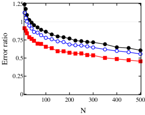
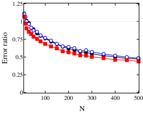
(a)	(b)

Figure 2: The SSEP error ratio vs. system size $N$. In (a), we show the error ratio $e_{N}$ (see text) for the estimated density at $x=0.3$ (solid discs), $x=0.5$ (open circles), and $x=0.8$ (squares). In (b), we show the error ratio for the near-neighbor product $\sigma_{[xN]}\cdot\sigma_{[xN]+1}$ with $x=0.5$ (solid discs), and for the products $\sigma_{[xN]}\cdot\sigma_{[yN]}$ with $(x,y)=(0.4,0.7)$ (open circles) and $(x,y)=(0.2,0.9)$ (squares). The errors are estimated using batched means estimators [18]. The parameters are $\alpha=2$, $\beta=0.1$, $\delta=0.3$, and $\gamma=1$.

Fig. 3 shows the error ratios for the occupation numbers $\sigma_{[xN]}$ as as functions of spatial location $x\in(0,1)$, for $N\in\{50,100,500\}$. As can be seen, the error ratio has a strong dependence on spatial location, nearly vanishing at the boundaries but quickly attaining a near-linear profile in the interior of the domain. The figure show that some degrees of freedom couple better than others, and that sites in a “boundary layer” near the reservoirs couple especially well. An explanation is that in order for the two processes to couple at, say, site $1$, we need only that their occupation numbers at site 1 agree, whereas for coupled moves to occur in in the interior of the system requires that the occupation numbers of two neighboring sites agree. In any case, despite this dependence on spatial location, overall the coupling control variate has improved the accuracy of MCMC estimates by a factor of $\gtrsim 40\%$ for $N\approx 500$.

We note that the coupling control variate estimator can be implemented with overhead of less than twice the running time of a single SSEP simulation. If we run two independent copies of SSEP simulations and average the results, the standard error of the resulting estimate will decrease by a factor of $1/\sqrt{2}\approx 0.7$, i.e., a 30% gain. We see that for single-site density estimates, the coupling control variate offers a noticeable improvement over simply running more copies of the simulation, and performs significantly better for two-site estimates.

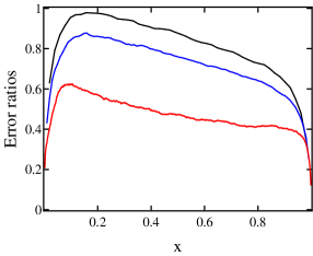
Figure 3: The SSEP error ratio for the occupation number $\sigma_{[xN]}$ as a function of location $x$. The curves are, from top to bottom, $N=50,100,500$. The parameters are $\alpha=2$, $\beta=0.1$, $\delta=0.3$, and $\gamma=1$.

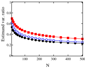
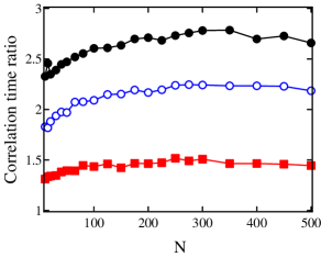
(a)	(b)

Figure 4: The variance and correlation time components of the error ratio for the SSEP. In (a), we show the factor $e_{var;N}$, as defined in Eq. (16), for $\phi=\sigma_{[xN]}$ with $x=0.3$ (solid discs), $x=0.5$ (open circles), and $x=0.8$ (squares). In (b), we show the corresponding ratios of correlation times. Correlation times are computed by checking numerically that Kubo scaling (4) is in effect (batched means estimates of the estimator error for integration times $T\in[10^{5},10^{7}]$ show that the mean squared error $\sim T^{-1/2}$). Then, the correlation time is “reverse-engineered” using the Kubo formula, and spot-checked by direct computation of time correlation functions. Variances are computed by time averaging for $10^{8}$ time units. The parameters are $\alpha=2$, $\beta=0.1$, $\delta=0.3$, and $\gamma=1$.

The Kubo formula (4) tells us that when the simulation time $T$ is sufficiently large, the error ratio (15) can be written as a product of two factors:

$$e_{N}[\phi] \approx\left(\frac{{\rm Var}\big{[}\phi(\sigma)-\phi(\eta)\big{]}}{{\rm Var}\big{[}\phi(\sigma)\big{]}}\right)^{1/2}\cdot\left(\frac{\tau_{couple}}{\tau}\right)^{1/2}$$ (16)

$$=e_{var;N}[\phi]\cdot e_{\tau;N}[\phi]~{}.$$

The reasoning in Sect. 1.2 suggests that the error ratio $e_{N}$ reflects both the gain in the first factor $e_{var;N}$ by reducing variance, and possible loss due to an increase in the second factor $e_{\tau;N}$, by increasing correlation times. To assess the situation, we have plotted $e_{var,N}[\phi]$, with $\phi=\sigma_{xN}$ for a few locations $x$, in Fig. 4(a). This curve should coincide with the plot of $e_{N}$ in Fig. 2(a) if the correlation time of the SSEP were equal to that of the coupling control variate. Instead, we find that $e_{var;N}<e_{N}$. Fig. 4(b) shows the ratio of integrated autocorrelation times. As can be seen, the coupling control variate may increase correlation times at the same time that it reduces variance. Here, the reduced variance wins over the increased correlation time.

2.2 KMP model

The second model we consider is the Kipnis-Marchioro-Presutti (KMP) model [9]. This is a stochastic idealization of a chain of $N$ coupled harmonic oscillators placed at the vertices of a regular lattice. We think of the $i$th oscillator as having energy $\varepsilon_{i}$, given by a nonnegative real number, so that the state space is $\Omega=[0,\infty)^{N}$. Note that unlike the SSEP, $\Omega$ is uncountable. At sites 0 and $N+1$, we place “heat baths” with temperature $T_{L}$ and $T_{R}$, respectively. There are thus $N+1$ bonds in the system, linking site $i$ with $i\pm 1$ for $i=1,\cdots,N$. Associated with each bond is an independent exponential clock of rate 1. If the clock for the bond $(i,i+1)$ rings and $1\leq i\leq N-1$, then the energies of oscillators $i$ and $i+1$ are pooled together and redistributed randomly, i.e., $\varepsilon_{i}^{+}=U\cdot(\varepsilon_{i}^{-}+\varepsilon_{i+1}^{-})$ and $\varepsilon_{i+1}^{+}=(1-U)\cdot(\varepsilon_{i}^{-}+\varepsilon_{i+1}^{-})$, where $U$ is a uniform random variable on $[0,1]$ independent of everything else, $\varepsilon^{+}$ denotes energy after the redistribution, and $\varepsilon^{-}$ denotes the prior energy. If the clock for the bond $i=0$ rings, $\varepsilon_{1}$ jumps to a new energy level $u$ with probability density $\beta_{L}e^{-\beta_{L}u},\beta_{L}=1/T_{L}$. Similarly for the bond $(N,N+1)$, but with parameter $\beta_{R}=1/T_{R}$. Notice that the dynamics conserves energy except at sites 1 and $N$, just as the interior dynamics of the SSEP conserves particle number.

The KMP process provide a simple microscopic model of heat conduction. When $T_{L}=T_{R}=T_{0}$, the system attains thermal equilibrium: the dynamics satisfies detailed balance, the stationary distribution $P_{N}$ is a product of Gibbs distributions with densities $\beta_{0}e^{-\beta_{0}\varepsilon}$ ($\beta_{0}=1/T_{0}$), and the temperature at all sites is equal to $T_{0}$. When $T_{L}\neq T_{R}$, we have a linear temperature profile

$$T(x)=T_{L}\cdot(1-x)+T_{R}\cdot x~{},\qquad x\in(0,1)~{},$$ (17)

where $T(x)=\lim_{N\to\infty}{\mathbb{E}}_{N}[\varepsilon_{[xn]}]$. This non-constant profile reflects the flow of a nonzero energy current through the system. The spatial correlations have a similar scaling as the SSEP [2]: the limit

$$c(x,y)=\lim_{N\to\infty}N~{}{\rm Cov}_{N}\big{(}\varepsilon_{[xN]},\varepsilon_{[yN]}\big{)}$$

exists, and

$$c(x,y)\propto(T_{R}-T_{L})^{2}\cdot x(1-y)\ ,\qquad 0<x<y<1\ .$$

Like the SSEP, ${\rm Cov}_{N}(\varepsilon_{[xN]},\varepsilon_{[yN]})=O(1/N)$. Thus, one encounters similar difficulties when estimating spatial correlations numerically.

It has been shown that the KMP model attains LTE as $N\to\infty$, i.e. $k$-site marginals converge to a product of Gibbs distributions, with a local temperature $T(x)$ given by the linear profile above. This suggests that we use

$$Q_{N}(\varepsilon)=\prod_{i=1}^{N}\beta_{i}e^{-\beta_{i}\varepsilon_{i}}~{},$$ (18)

where $\beta_{i}=1/T(x_{i})$, as approximate stationary distribution. A simple coupling of the KMP process to itself is also available: given two copies of the KMP process, we make the same bonds “ring” at the same time. For interior bonds, we use the same uniform random numbers $U$ to split energy in both copies; for heat baths, we set the boundary sites to the same new energy. The coupling is illustrated in Fig. 5: it entails having the $\tilde{\varepsilon}$ process use the same “randomness” as the $\varepsilon$ process to redistribute energy between nearby sites.

Figure 5: Illustration of the KMP coupling. Because the interaction conserves energy, the point $(X_{i},X_{i+1})$ is constrained to lie on the line $X_{i}+X_{i+1}=\mbox{const}$ both before and after the interaction.

One difference from the SSEP is that the KMP model has an uncountable state space, so the algorithm described in Sect. 1 requires slight modification. This is straightforward for Markov jump processes with transition densities: one can simply replace the ratio of transition rate coefficients $R_{X}$ in Eq. (8) with the ratio of the corresponding densities. The KMP process does not only have an uncountable state space, though — it also has singular transition rate measures (this is a consequence of energy conservation). Nonetheless, it can be checked that the ratios are well-defined in this case, and yield the following Metropolis ratios:

Interaction resulting in $(\varepsilon_{i},\varepsilon_{j})\mapsto(\varepsilon^{\prime}_{i},\varepsilon^{\prime}_{j})$, $|i-j|=1$	$Z_{ij}=\exp\Big{(}[\beta_{i}\varepsilon_{i}+\beta_{j}\varepsilon_{j}]-[\beta_{i}\varepsilon^{\prime}_{i}+\beta_{j}\varepsilon^{\prime}_{j}]\Big{)}$
Left heat bath setting $\varepsilon_{1}\mapsto\varepsilon^{\prime}_{1}$	$Z_{L}=\exp\big{(}(\beta_{L}-\beta_{1})\cdot(\varepsilon^{\prime}_{1}-\varepsilon_{1})\big{)}$
Right heat bath setting $\varepsilon_{n}\mapsto\varepsilon^{\prime}_{n}$	$Z_{R}=\exp\big{(}(\beta_{R}-\beta_{n})\cdot(\varepsilon^{\prime}_{n}-\varepsilon_{n})\big{)}$

Applying the algorithm in Sect. 1.2 with these ratios yields a coupling control variate which preserves the local equilibrium distribution $Q_{N}$.

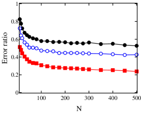
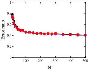
(a)	(b)

Figure 6: The KMP error ratio as a function of system size $N$. In (a), we show the error ratio for the estimated mean energies at $x=0.3$ (solid discs), $x=0.5$ (open circles), and $x=0.8$ (squares) as functions of $N$. In (b), we show the error ratio for the near-neighbor product $\varepsilon_{[xN]}\cdot\varepsilon_{[xN]+1}$ with $x=0.5$ (solid discs), and for the products $\varepsilon_{[xN]}\cdot\varepsilon_{[yN]}$ with $(x,y)=(0.4,0.7)$ (open circles) and $(x,y)=(0.2,0.9)$ (squares). The errors are estimated using batched means estimator. The parameters are $T_{L}=10$ and $T_{R}=100$.

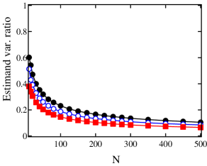
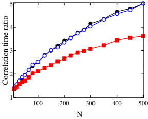
(a)	(b)

Figure 7: The variance and correlation time components of the error ratio for the KMP process. In (a), we show the factor $e_{var;N}$, as defined in Eq. (16), for $\phi=\varepsilon_{[xN]}$ for $x=0.3$ (solid discs), $x=0.5$ (open circles), and $x=0.8$ (squares). In (b), we show the corresponding “reverse-engineered” ratio of correlation times. The parameters are $T_{L}=10$ and $T_{R}=100$.

Numerical results. Fig. 6(a) shows the error ratios for various sites in the KMP model. As is the case for the SSEP, the coupling control variate significantly reduces the variance of the estimator. In contrast to the SSEP, the amount by which the error is reduced depends more strongly on location, ranging from 20 to 60%. Fig. 7(b) shows the error ratios for the products $\varepsilon_{[xN]}\cdot\varepsilon_{[yN]}$ for pairs $(x,y)$ located at various distances. These ratios are much more consistent and tend to $\approx 40\%$ for the range of $N$ tested.

Fig. 7(a) shows the corresponding factor $e_{var;N}$. As in the case of the SSEP, $e_{var;N}$ is strictly smaller than the error ratio $e_{N}$; at the same time, the ratio $e_{\tau;N}$ of correlation times increase; see Fig. 7(b). Thus, Metropolis rejections can have a dramatic effect on the correlation time of the coupling control variate. Despite that, the overall performance of the coupling control variate estimator is quite good: even at its worst, the accuracy has been improved by 40%.

Conclusion

We have shown that Markov couplings, when available, can be used effectively to improve the accuracy of Markov chain Monte Carlo calculations. This method useful in situations where the stationary distribution is not known explicitly, as in the case of nonequilibrium transport models. As shown by the examples considered in this paper, good candidates for approximate stationary distribution can be found based on physical reasoning, and when an effective coupling is available for the Markov process at hand, one can construct an effective coupling control variate.

The numerical results suggest various directions for improvement. In particular, the observation that coupling control variate has larger correlation times than the original process suggests that one try to “trade” variance for correlation time. However, simple ideas like resampling the energy of random sites at random times, as in heat bath / partial resampling, may very well increase variance more than it decreases correlation time, resulting in a net gain of error. A related issue is the dependence of the estimator error ratio on observables: in many applications, it is desirable to be able to optimize the error ratio only for observables of interest. (One does not expect to be able to have small error ratios for all observables unless the approximate and true stationary distributions are close in the total variation norm.)

Finally, we mention that it might be possible to use related coupling methods for sensitivity analysis. If the Markov process depends on parameters $\theta$, then the observable $\phi$ in Eq. (6) becomes $\phi_{\theta}$ and the sensitivities are derivatives of $\phi_{\theta}$ with respect to $\theta$. Sensitivities are used, for example, in numerical computation of optimal stochastic controls in situations where the curse of dimensionality makes dynamic programming impractical. If there is a known formula for the stationary distribution $P_{\theta}$, two common methods for evaluating sensitivities, the common random variables (or same paths) method and the likelihood ratio (or score function) methods. Glynn [6] and others have generalizations of the likelihood ratio method to situations where $T$ is known but not $P$. It also might be helpful to have such a generalization of the same paths method.

Acknowledgments.

We thank Peter Glynn for pointing out the references [6, 17, 20]. JG was supported in part by the Applied Mathematical Sciences Program of the U.S. Department of Energy under Contract DEFG0200ER25053. KL was supported in part by an NSF Mathematical Sciences Postdoctoral Fellowship.

References

- [1] T. W. Anderson, The Statistical Analysis of Time Series, John Wiley & Sons, New York (1971)
- [2] L. Bertini, D. Gabrielli, and J. L. Lebowitz, “Large deviations for a stochastic model of heat flow,” J. Stat. Phys. 121 (2005) pp. 843–885
- [3] S. R. de Groot and P. Mazur, Non-Equilibrium Thermodynamics, North-Holland (1962)
- [4] B. Derrida, “Non-equilibrium steady states: fluctuations and large deviations of the density and of the current,” J. Stat. Mech. (2007) P07023
- [5] D. T. Gillespie, “Exact stochastic simulation of coupled chemical-reactions,” J. Phys. Chem. 81 (1977) pp. 2340–2361
- [6] P. W. Glynn and P. L’Ecuyer, “Likelihood ratio gradient estimation for stochastic recursions,” Adv. in Appl. Probab. 27 (1995) pp. 1019–1053
- [7] J. M. Hammersley and D. C. Handscomb, Monte Carlo Methods, John Wiley and Sons (1964)
- [8] J. A. Izaguirre and S. S. Hampton, “Shadow hybrid Monte Carlo: an efficient propagator in phase space of macromolecules,” J. Comp. Phys. 200 (2004) pp. 581-604
- [9] C. Kipnis, C. Marchioro, and E. Presutti, “Heat flow in an exactly solvable model,” J. Stat. Phys. 27 (1982)
- [10] M. H. Kalos and P. A. Whitlock, Monte Carlo Methods, Wiley (1986)
- [11] Y. Le Jan, “On isotropic Brownian motion,” Z. Wahr. Verw. Geb. 70 (1985) pp. 609–620
- [12] T. M. Liggett, Interacting Particle Systems, Springer-Verlag (1985)
- [13] K. K. Lin and L.-S. Young, “Correlations in nonequilibrium steady states of random-halves models,” J. Stat. Phys. 128 (2007) pp. 607–639
- [14] T. Lindvall, Lectures on the Coupling Method, Wiley (1992)
- [15] R. L. Pinto and R. M. Neal, “Improving Markov chain Monte Carlo estimators by coupling to an approximating chain,” Technical Report No. 0101, Dept. of Statistics, University of Toronto (2001)
- [16] J. Propp and D. Wilson, “Exact sampling with coupled Markov chains and applications to statistical mechanics,” Random Structures and Algorithms 9 (1995) pp. 223–252
- [17] A. P. Sharon and B. L. Nelson, “Analytic and external control variates for queueing network simulation,” J. Oper. Res. Soc. 39 (1998) pp. 595–602
- [18] A. D. Sokal, “Monte Carlo Methods in Statistical Mechanics: Foundations and New Algorithms,” in Functional Integration, NATO Adv. Sci. Inst. Ser. B Phys. 361 (1997) pp. 131–192
- [19] H. Spohn, “Long range correlations for stochastic lattice gases in a non-equilibrium steady state,” J. Phys. A 16 (1983) pp. 4275–4291
- [20] M. R. Taaffe and S. A. Horn, “External control variance reduction for nonstationary simulation,” Proc. 1983 Winter Simulation Conference, S. Roberts, J. Banks, B. Schmeiser, Eds. (1983)