Variational and perturbative formulations of QM/MM free energy with mean-field embedding and its analytical gradients

Abstract

Conventional quantum chemical solvation theories are based on the mean-field embedding approximation. That is, the electronic wavefunction is calculated in the presence of the mean field of the environment. In this paper a direct quantum mechanical/molecular mechanical (QM/MM) analog of such a mean-field theory is formulated based on variational and perturbative frameworks. In the variational framework, an appropriate QM/MM free energy functional is defined and is minimized in terms of the trial wavefunction that best approximates the true QM wavefunction in a statistically averaged sense. Analytical free energy gradient is obtained, which takes the form of the gradient of effective QM energy calculated in the averaged MM potential. In the perturbative framework, the above variational procedure is shown to be equivalent with the first-order expansion of the QM energy (in the exact free energy expression) about the self-consistent reference field. This helps understand the relation between the variational procedure and the exact QM/MM free energy as well as existing QM/MM theories. Based on this, several ways are discussed for evaluating non-mean-field effects (i.e., statistical fluctuations of the QM wavefunction) that are neglected in the mean-field calculation. As an illustration, the method is applied to an S_N2 Menshutkin reaction in water, $\mathrm{NH_{3}+CH_{3}Cl\rightarrow NH_{3}CH_{3}^{+}+Cl^{-}},$ for which free energy profiles are obtained at the HF, MP2, B3LYP, and BH&HLYP levels by integrating the free energy gradient. Non-mean-field effects are evaluated to be $<0.5$ kcal/mol using a Gaussian fluctuation model for the environment, which suggests that those effects are rather small for the present reaction in water.

I Introduction

A combined quantum mechanical/molecular mechanical (QM/MM) method is a powerful computational tool for studying chemical reactions in solution and in biological systems.Warshel (1991); Cramer (2002) It treats a chemically active part of the entire system with accurate QM methods while the rest of the system with MM force fields. The quality of a given QM/MM calculation depends primarily on the electronic structure method used. In the calculation of statistical properties like free energy, it is also important to adequately sample the relevant phase space.Klahn et al. (2005) However, this phase space sampling is very demanding computationally, because one needs to calculate QM electronic energy for a large number of statistical samples. One can ensure sufficient statistics by using fast semiempirical methods, but the resulting energetics may be less satisfactory than obtained with ab initio methods. On the other hand, highly correlated QM methods require too much computational time and thus it becomes difficult to explore the phase space.

A variety of approaches have been proposed in order to address the above trade-off between accuracy and efficiency. One approach is a family of dual-level methods, in which a classical or semiempirical potential is used for statistical sampling and an accurate QM method for energetic corrections.Muller and Warshel (1995); Bentzien et al. (1998); Strajbl et al. (2002); Rosta et al. (2006); Wood et al. (1999); Sakane et al. (2000); Wood et al. (2002); Rod and Ryde (2005a, b); Ruiz-Pernia et al. (2004); Valiev et al. (2007); Crespo et al. (2005) Another approach is to introduce some approximation to the QM–MM electrostatic interactions in order to reduce the number of QM calculations. Our main interest in this paper is in the second approach above. In particular, we are concerned with the following three embedding schemes that prescribe how to calculate the QM wavefunction in the MM environment:

(1) Gas-phase embedding scheme. This scheme totally neglects electrostatic perturbations of the MM environment on the QM subsystem. The QM wavefunction is calculated a priori in the gas phase, and the resulting charge density or partial charges are embedded into the MM environment. The reaction path is also determined by the gas-phase calculation. The free energy profile in solution is obtained via free energy perturbation (FEP) calculations along the pre-determined reaction path. This approach was first utilized by Jorgensen and co-workersChandrasekhar et al. (1985); Jorgensen (1989); Blake and Jorgensen (1991); Severance and Jorgensen (1992) to study organic reactions in solution, and later by Kollman and co-workersStanton et al. (1998); Kuhn and Kollman (2000); Kollman et al. (2001) to study enzyme reactions. It should be noted however that this approach may not be appropriate for a certain class of enzyme reactions.Zhang et al. (1999)

(2) Mean-field embedding scheme. This method calculates the QM wavefunction in the presence of the mean field of the environment. The averaged polarization (or distortion) of the QM wavefunction is thus correctly taken into account, while statistical fluctuations of the QM wavefunction are totally neglected. Indeed, this mean-field approximation has been the basis of many conventional solvation models like the PCMTomasi and Persico (1994); Tomasi et al. (2005) and RISM-SCFTen-no et al. (1994); Sato et al. (1996, 2000); Hirata (2004) methods. The mean-field idea has also been applied to the QM/MM framework by several authors. For example, Aguilar and co-workers Galvan et al. (2003a, b, 2004); Sanchez et al. (2002); Galvan et al. (2006) performed geometry optimization on an approximate QM/MM free energy surface using the averaged solvent electrostatic potential (ASEP)/MD method. More recently, the mean-field idea was exploited by Warshel and co-workersRosta et al. (2008) in order to accelerate QM/MM calculation of solvation free energy.

(3) Polarizable embedding scheme. This method first develops a polarizable model of the QM subsystem and then embeds the resulting model into the MM environment. The polarizable QM model can be developed, for example, by Taylor expanding the QM electronic energy up to second order. Morita and Kato (1997, 1998); Naka et al. (1999a); Lu and Yang (2004); Hu et al. (2007a, 2008); Hu and Yang (2008); Higashi and Truhlar (2008) The QM/MM minimum free energy path (MFEP) method by Yang and co-workers Lu and Yang (2004); Hu et al. (2007a, 2008); Hu and Yang (2008) is based on this perturbative expansion idea, which has been applied to chemical reactions in solution and enzymes. Among the three embedding schemes above, the polarizable one is most accurate by allowing statistical fluctuations of the QM wavefunction.

The first goal of this paper is to formulate the mean-field embedding scheme above by starting from a variational principle for the QM/MM free energy (Sec. II.2). As mentioned above, conventional solvation models are based on the mean-field embedding approximation. They often start with a variational principle for the following free energy Tomasi and Persico (1994); Tomasi et al. (2005); Ángyán (1992)

$$A(\mathbf{r}_{\mathrm{QM}})=\langle\Psi|\hat{H}_{\mathrm{QM}}|\Psi\rangle+\Delta A_{\mathrm{solv}}[\Psi].$$ (1)

Minimization of $A(\mathbf{r}_{\mathrm{QM}})$ in terms of $\Psi$ gives a nonlinear Schrödinger equation for $\Psi$ that is subject to the mean field of the environment. Very often, analytical gradient of free energy, $\partial A(\mathbf{r}_{\mathrm{QM}})/\partial\mathbf{r}_{\mathrm{QM}}$, is obtained by utilizing the variational nature of $A(\mathbf{r}_{\mathrm{QM}})$. Since those solvation models are quite successful in studying solution-phase chemistry, it is natural to try to extend them to the QM/MM framework. The main benefits of this extension are as follows. First, QM/MM models can describe inhomogeneous as well as homogeneous environments on an equal theoretical footing. This makes it more straightforward to compare the chemical reactivity of a system in different environments (e.g., in solution and enzymes). Second, since the mean-field QM wavefunction is calculated only for a “batch” of MM configurations, the number of QM calculations can be made significantly smaller than a direct QM/MM statistical calculation. As mentioned above, such a mean-field QM/MM approach has been explored by several authors in the literature. For example, ÁngyánÁngyán (1992) discussed such a method quite a few years ago based on a variational principle and linear-response approximation (LRA). More recently, Kato and co-workersHigashi et al. (2007a, b) developed the QM/MM LRFE method using a different type of variational/LRA idea and applied it to chemical reactions in solution and enzymes. On the other hand, Aguilar and co-workersGalvan et al. (2003b) took a different approach in the ASEP/MD method, where they did not invoke a variational principle nor LRA but rather approximated the free energy gradient as follows:

$$\frac{\partial A(\mathbf{r}_{\mathrm{QM}})}{\partial\mathbf{r}_{\mathrm{QM}}}=\left\langle\frac{\partial E(\mathbf{r}_{\mathrm{QM}},\mathbf{r}_{\mathrm{MM}})}{\partial\mathbf{r}_{\mathrm{QM}}}\right\rangle\simeq\frac{\partial}{\partial\mathbf{r}_{\mathrm{QM}}}\langle E(\mathbf{r}_{\mathrm{QM}},\mathbf{r}_{\mathrm{MM}})\rangle.$$ (2)

Here, $E(\mathbf{r}_{\mathrm{QM}},\mathbf{r}_{\mathrm{MM}})$ is the total energy of the QM/MM system and $\langle\cdots\rangle$ denotes the statistical average over MM degrees of freedom. Note that in Eq. (2) “the average of the energy gradient” (the exact expression) is replaced by “the gradient of the averaged energy” in the spirit of the mean-field approximation. While Aguilar et al. demonstrated its accuracy via comparison with direct QM/MM calculations,Galvan et al. (2003b) the detailed derivation of Eq. (2) was not provided and it was used as an ansatz. Therefore, our first aim in this paper is (i) to formulate a mean-field QM/MM framework by starting from a variational principle (but not invoking the LRA), (ii) obtain analytical gradient of the associated free energy, and (iii) discuss a possible rationale for the approximate gradient in Eq. (2).

The second goal of this paper is to understand the relation of the above variational/mean-field procedure with the underlying exact QM/MM free energy as well as existing QM/MM theories (Secs. II.3 and II.4). First, it is shown that the above variational procedure is equivalent with the first-order expansion of effective QM energy (in the exact free energy expression) about the self-consistent reference field. As mentioned above, the QM/MM-MFEP method Hu et al. (2007a, 2008) is based on this type of perturbative expansions. Therefore, it is interesting to compare the present approach with the QM/MM-MFEP method in detail (Appendix C). From this comparison it follows that the variational procedure is essentially equivalent with Model 3 of the QM/MM-MFEP method with charge response kernel $\chi$ neglected. Note however that the full version of Model 3 includes that response kernel $\chi$ and thus it is more accurate by describing statistical fluctuations of the QM wavefunction. Therefore, in Sec. II.4 we also discuss several possible ways for evaluating such non-mean-field effects on top of the variational/mean-field calculation.

As an illustration, the present method is applied to an S_N2 reaction in water (Sec. III). Free energy profiles are obtained by integrating the free energy gradient and they are compared with free energy perturbation (FEP) results. Non-mean-field effects are also evaluated using a Gaussian fluctuation model for the environment. The obtained results suggest that the non-mean-field effects are rather small for the present reaction in water.

II Methodology

II.1 The underlying QM/MM free energy

We consider the following QM/MM free energy (or the potential of mean forces acting on QM atoms)

$$A(\mathbf{R})=-\frac{1}{\beta}\ln\int d\mathbf{R}^{+}\exp\{-\beta E(\mathbf{R},\mathbf{R}^{+})\},$$ (3)

where $\mathbf{R}$ and $\mathbf{R}^{+}$ are Cartesian coordinates of the QM and MM atoms, respectively, $\beta=1/k_{B}T$ is the reciprocal temperature, and $E(\mathbf{R},\mathbf{R}^{+})$ is the total energy given by

$$E(\mathbf{R},\mathbf{R}^{+})=\mathcal{E}_{\mathrm{QM}}(\mathbf{R},\mathbf{v}_{\mathrm{MM}}(\mathbf{R},\mathbf{R}^{+}))+\mathcal{E}_{\mathrm{MM}}(\mathbf{R},\mathbf{R}^{+}).$$ (4)

Here, $\mathcal{E}_{\mathrm{QM}}$ is the electronic energy of the QM subsystem in the presence of an external electrostatic field (called the effective QM energy). In the standard electronic embedding scheme, it is defined via the following Schrödinger equation

$$[\hat{H}_{\mathrm{QM}}+\int d\mathbf{x}\hat{\rho}(\mathbf{x})v^{\prime}(\mathbf{x})]|\Psi[\mathbf{R},v^{\prime}]\rangle=\mathcal{E}_{\mathrm{QM}}[\mathbf{R},v^{\prime}]|\Psi[\mathbf{R},v^{\prime}]\rangle$$ (5)

(note that the prime symbol will be attached on variables and functions of “dummy” nature). $\hat{H}_{\mathrm{QM}}$ is the QM Hamiltonian in the gas phase, $\hat{\rho}(\mathbf{x})$ is the QM charge density operator,

$$\hat{\rho}(\mathbf{x})=\sum^{\mathrm{nuc}}_{a}Z_{a}\delta(\mathbf{x}-\mathbf{R}_{a})-\sum^{\mathrm{ele}}_{i}\delta(\mathbf{x}-\hat{\mathbf{r}}_{i}),$$ (6)

and $v^{\prime}(\mathbf{x})$ is an (arbitrary) external electrostatic field. In this paper we will utilize a discretized approximation to Eq. (5) given by

$$[\hat{H}_{\mathrm{QM}}+\sum_{a}\hat{Q}_{a}v^{\prime}_{a}]|\Psi(\mathbf{R},\mathbf{v}^{\prime})\rangle=\mathcal{E}_{\mathrm{QM}}(\mathbf{R},\mathbf{v}^{\prime})|\Psi(\mathbf{R},\mathbf{v}^{\prime})\rangle,$$ (7)

where $\{\hat{Q}_{a}\}$ are a set of “partial charge” operators associated with QM atoms $\{\mathbf{R}_{a}\}$, and $v^{\prime}_{a}=v^{\prime}(\mathbf{R}_{a})$. The motivation for using Eq. (7) is that the external field can be parametrized by an $N$-dimensional vector $\mathbf{v}^{\prime}=(v^{\prime}_{1},\ldots,v^{\prime}_{N})$, where $N$ is the number of QM atoms. This fact makes the following discussion somewhat simpler. Nevertheless, we stress that there is no fundamental difficulty in using the original Schrödinger equation in Eq. (5); see Appendix A for such a formulation. In Appendix B, we summarize the present definition of the partial charge operator $\hat{\mathbf{Q}}=(\hat{Q}_{1},\ldots,\hat{Q}_{N})$ based on the electrostatic potential (ESP) fitting procedure.Bayly et al. (1993)

Now going back to Eq. (4), $\mathbf{v}_{\mathrm{MM}}(\mathbf{R},\mathbf{R}^{+})=(v_{\mathrm{MM},1},\ldots,v_{\mathrm{MM},N})$ are MM electrostatic potentials acting on QM atoms,

$$v_{\mathrm{MM},a}=v_{\mathrm{MM}}(\mathbf{R}_{a},\mathbf{R}^{+}),$$ (8)

where

$$v_{\mathrm{MM}}(\mathbf{x},\mathbf{R}^{+})=\sum_{l}\frac{q_{l}^{\mathrm{MM}}}{|\mathbf{x}-\mathbf{R}^{+}_{l}|}$$ (9)

with $\{q^{\mathrm{MM}}_{l}\}$ being partial charges of the MM atoms. $\mathcal{E}_{\mathrm{MM}}(\mathbf{R},\mathbf{R}^{+})$ is the sum of the van der Waals interactions between QM–MM subsystems and the internal energy of the MM subsystem,

$$\mathcal{E}_{\mathrm{MM}}(\mathbf{R},\mathbf{R}^{+})=E_{\mathrm{QM/MM}}^{\mathrm{vdw}}(\mathbf{R},\mathbf{R}^{+})+E_{\mathrm{MM}}(\mathbf{R}^{+}).$$ (10)

In the following we will sometimes drop the arguments of $\mathbf{v}_{\mathrm{MM}}$ and $\mathcal{E}_{\mathrm{MM}}$ for notational simplicity, i.e. $\mathbf{v}_{\mathrm{MM}}=\mathbf{v}_{\mathrm{MM}}(\mathbf{R},\mathbf{R}^{+})$ and $\mathcal{E}_{\mathrm{MM}}=\mathcal{E}_{\mathrm{MM}}(\mathbf{R},\mathbf{R}^{+})$.

II.2 Variational approach for mean-field embedding

The free energy in Eq. (3) may be rewritten as

$$A(\mathbf{R})=-\frac{1}{\beta}\ln\int d\mathbf{R}^{+}\exp\{-\beta[\langle\Psi(\mathbf{R},\mathbf{v}_{\mathrm{MM}})|\hat{H}_{\mathrm{QM}}+\hat{\mathbf{Q}}\cdot\mathbf{v}_{\mathrm{MM}}|\Psi(\mathbf{R},\mathbf{v}_{\mathrm{MM}})\rangle+\mathcal{E}_{\mathrm{MM}}]\},$$ (11)

by explicitly writing $\mathcal{E}_{\mathrm{QM}}(\mathbf{R},\mathbf{v}_{\mathrm{MM}})$ in terms of the QM wavefunction. Note that $\mathbf{v}_{\mathrm{MM}}$ always stands for $\mathbf{v}_{\mathrm{MM}}(\mathbf{R},\mathbf{R}^{+})$ as mentioned above. A direct evaluation of $A(\mathbf{R})$ is computationally demanding because $\Psi(\mathbf{R},\mathbf{v}_{\mathrm{MM}})$ depends on $\mathbf{R}^{+}$ through $\mathbf{v}_{\mathrm{MM}}=\mathbf{v}_{\mathrm{MM}}(\mathbf{R},\mathbf{R}^{+})$. To avoid repeated QM calculations, let us replace the true wavefunction $\Psi(\mathbf{R},\mathbf{v}_{\mathrm{MM}})$ by some trial one $\tilde{\Psi}(\mathbf{R})$ that best approximates the true wavefunction in a statistically averaged sense. To do so, we consider a free energy functional of the form

$$\tilde{A}[\mathbf{R},\tilde{\Psi}]=-\frac{1}{\beta}\ln\int d\mathbf{R}^{+}\exp\{-\beta[\langle\tilde{\Psi}|\hat{H}_{\mathrm{QM}}+\hat{\mathbf{Q}}\cdot\mathbf{v}_{\mathrm{MM}}|\tilde{\Psi}\rangle+\mathcal{E}_{\mathrm{MM}}]\}.$$ (12)

Since the following inequality holds by definition for arbitrary $\mathbf{v}_{\mathrm{MM}}=\mathbf{v}_{\mathrm{MM}}(\mathbf{R},\mathbf{R}^{+})$ [we assume that $\Psi(\mathbf{R},\mathbf{v}_{\mathrm{MM}})$ is the ground state of $\hat{H}_{\mathrm{QM}}+\hat{\mathbf{Q}}\cdot\mathbf{v}_{\mathrm{MM}}$],

$$\langle\Psi(\mathbf{R},\mathbf{v}_{\mathrm{MM}})|\hat{H}_{\mathrm{QM}}+\hat{\mathbf{Q}}\cdot\mathbf{v}_{\mathrm{MM}}|\Psi(\mathbf{R},\mathbf{v}_{\mathrm{MM}})\rangle\;\leqslant\;\langle\tilde{\Psi}(\mathbf{R})|\hat{H}_{\mathrm{QM}}+\hat{\mathbf{Q}}\cdot\mathbf{v}_{\mathrm{MM}}|\tilde{\Psi}(\mathbf{R})\rangle,$$ (13)

we obtain a variational principle for free energy

$$A(\mathbf{R})\leqslant\tilde{A}[\mathbf{R},\tilde{\Psi}].$$ (14)

Namely, $\tilde{A}[\mathbf{R},\tilde{\Psi}]$ is a strict upper bound on $A(\mathbf{R})$, and the best approximation to $A(\mathbf{R})$ is obtained by minimizing $\tilde{A}[\mathbf{R},\tilde{\Psi}]$ with respect to $\tilde{\Psi}$. This variational principle is indeed a direct QM/MM analog of the standard ones used in conventional solvation theories.Ángyán (1992); Tomasi and Persico (1994); Tomasi et al. (2005) By minimizing the following Lagrangian to account for the normalization of $\tilde{\Psi}$,

$$L[\mathbf{R},\tilde{\Psi},\lambda]=\tilde{A}[\mathbf{R},\tilde{\Psi}]-\lambda\{\langle\tilde{\Psi}|\tilde{\Psi}\rangle-1\},$$ (15)

we obtain the following stationary condition for $\tilde{\Psi}$:

$$\left[\hat{H}_{\mathrm{QM}}+\hat{\mathbf{Q}}\cdot\ll\mathbf{v}_{\mathrm{MM}}\gg_{\mathbf{Q}[\tilde{\Psi}]}\right]|\tilde{\Psi}\rangle=\lambda|\tilde{\Psi}\rangle.$$ (16)

Here $\ll\cdots\gg$ represents the statistical average over MM degrees of freedom,

$$\ll\cdots\gg_{\mathbf{Q}^{\prime}}=\frac{\int d\mathbf{R}^{+}e^{-\beta[\mathbf{Q}^{\prime}\cdot\mathbf{v}_{\mathrm{MM}}+\mathcal{E}_{\mathrm{MM}}]}(\cdots)}{\int d\mathbf{R}^{+}e^{-\beta[\mathbf{Q}^{\prime}\cdot\mathbf{v}_{\mathrm{MM}}+\mathcal{E}_{\mathrm{MM}}]}},$$ (17)

and $\mathbf{Q}[\Psi^{\prime}]=\langle\Psi^{\prime}|\hat{\mathbf{Q}}|\Psi^{\prime}\rangle$. [In this paper the double bracket $\ll\cdots\gg$ indicates that the average is of “classical” nature, i.e., it does not require repeated QM calculations.] Since Eq. (16) is nonlinear with respect to $\tilde{\Psi}$, it is usually solved via iteration. It follows from comparison between Eqs. (7) and (16) that $\tilde{\Psi}$ and $\lambda$ may be written as

$$\tilde{\Psi} = \Psi(\mathbf{R},\mathbf{v}^{\mathrm{sc}}),$$ (18a)

$$\lambda = \mathcal{E}_{\mathrm{QM}}(\mathbf{R},\mathbf{v}^{\mathrm{sc}}),$$ (18b)

where $\mathbf{v}^{\mathrm{sc}}$ is the self-consistent response field determined by

$$\mathbf{v}^{\mathrm{sc}}(\mathbf{R}) = \ll\mathbf{v}_{\mathrm{MM}}(\mathbf{R},\mathbf{R}^{+})\gg_{\mathbf{Q}^{\mathrm{sc}}},$$ (19a)

$$\mathbf{Q}^{\mathrm{sc}}(\mathbf{R}) = \langle\Psi^{\mathrm{sc}}|\hat{\mathbf{Q}}|\Psi^{\mathrm{sc}}\rangle,$$ (19b)

with $\Psi^{\mathrm{sc}}=\Psi(\mathbf{R},\mathbf{v}^{\mathrm{sc}})$. In this paper, Eq. (19) will be called the self-consistent (embedding) condition. The minimum value of the free energy functional is obtained by inserting $\tilde{\Psi}=\Psi^{\mathrm{sc}}$ into Eq. (12):

$$\min_{\tilde{\Psi}}\tilde{A}[\mathbf{R},\tilde{\Psi}] = -\frac{1}{\beta}\ln\int d\mathbf{R}^{+}\exp\{-\beta[\langle\Psi^{\mathrm{sc}}|\hat{H}_{\mathrm{QM}}+\hat{\mathbf{Q}}\cdot\mathbf{v}_{\mathrm{MM}}|\Psi^{\mathrm{sc}}\rangle+\mathcal{E}_{\mathrm{MM}}]\}$$ (20)

$$= \langle\Psi^{\mathrm{sc}}|\hat{H}_{\mathrm{QM}}|\Psi^{\mathrm{sc}}\rangle+\Delta A_{\mathrm{MM}}(\mathbf{R},\mathbf{Q}^{\mathrm{sc}})$$

$$\equiv A^{\mathrm{MF}}(\mathbf{R}),$$

where $\Delta A_{\mathrm{MM}}$ is defined by

$$\Delta A_{\mathrm{MM}}(\mathbf{R},\mathbf{Q}^{\prime})=-\frac{1}{\beta}\ln\int d\mathbf{R}^{+}e^{-\beta[\mathbf{Q}^{\prime}\cdot\mathbf{v}_{\mathrm{MM}}+\mathcal{E}_{\mathrm{MM}}]}.$$ (21)

Note that $\langle\Psi^{\mathrm{sc}}|\hat{H}_{\mathrm{QM}}|\Psi^{\mathrm{sc}}\rangle$ has been extracted from the integral over $\mathbf{R}^{+}$ since it is independent of $\mathbf{R}^{+}$. By the last line of Eq. (20), we define the QM/MM free energy with mean-field embedding approximation, $A^{\mathrm{MF}}(\mathbf{R})$.

The analytical gradient of $A^{\mathrm{MF}}(\mathbf{R})$ can be obtained using a standard procedure as follows. First, we rewrite the $A^{\mathrm{MF}}(\mathbf{R})$ in terms of the Lagrangian,

$$A^{\mathrm{MF}}(\mathbf{R})=\tilde{A}[\mathbf{R},\Psi^{\mathrm{sc}}]=L[\mathbf{R},\Psi^{\mathrm{sc}},\lambda^{\mathrm{sc}}]$$ (22)

with $\lambda^{\mathrm{sc}}=\mathcal{E}_{\mathrm{QM}}(\mathbf{R},\mathbf{v}^{\mathrm{sc}})$. Recalling that $L[\mathbf{R},\tilde{\Psi},\lambda]$ is stationary with respect to $\tilde{\Psi}$ and $\lambda$, we obtain

$$\frac{\partial}{\partial\mathbf{R}}A^{\mathrm{MF}}(\mathbf{R})=\left.\frac{\partial L[\mathbf{R},\tilde{\Psi},\lambda]}{\partial\mathbf{R}}\right|_{\tilde{\Psi}=\Psi^{\mathrm{sc}},\lambda=\lambda^{\mathrm{sc}}},$$ (23)

where the $\mathbf{R}$ derivative in the right-hand side does not act on $\tilde{\Psi}$ nor $\lambda$. We then obtain the analytical gradient in Eq. (33), which will be discussed in the next section.

II.3 Perturbative approach for mean-field embedding

$A^{\mathrm{MF}}(\mathbf{R})$ in Eq. (20) can also be obtained from the exact $A(\mathbf{R})$ in Eq. (3) by Taylor expanding the effective QM energy $\mathcal{E}_{\mathrm{QM}}(\mathbf{R},\mathbf{v}_{\mathrm{MM}})$ up to first order:

$$\mathcal{E}_{\mathrm{QM}}(\mathbf{R},\mathbf{v}_{\mathrm{MM}})\simeq\mathcal{E}_{\mathrm{QM}}(\mathbf{R},\mathbf{v}^{\circ})\\ +\left.\frac{\partial\mathcal{E}_{\mathrm{QM}}(\mathbf{R},\mathbf{v}^{\prime})}{\partial\mathbf{v}^{\prime}}\right|_{\mathbf{v}^{\prime}=\mathbf{v}^{\circ}}\cdot(\mathbf{v}_{\mathrm{MM}}-\mathbf{v}^{\circ}).$$ (24)

Here, $\mathbf{v}^{\circ}=\mathbf{v}^{\circ}(\mathbf{R})$ is an arbitrary reference potential that is assumed to be independent of $\mathbf{R}^{+}$. Using the following Hellman-Feynman theorem for $\mathcal{E}_{\mathrm{QM}}$,

$$\frac{\partial\mathcal{E}_{\mathrm{QM}}(\mathbf{R},\mathbf{v}^{\prime})}{\partial\mathbf{v}^{\prime}} = \langle\Psi(\mathbf{R},\mathbf{v}^{\prime})|\hat{\mathbf{Q}}|\Psi(\mathbf{R},\mathbf{v}^{\prime})\rangle$$ (25)

$$\equiv \mathbf{Q}(\mathbf{R},\mathbf{v}^{\prime}),$$

and introducing the internal QM energy as

$$E_{\mathrm{QM}}(\mathbf{R},\mathbf{v}^{\prime})=\langle\Psi(\mathbf{R},\mathbf{v}^{\prime})|\hat{H}_{\mathrm{QM}}|\Psi(\mathbf{R},\mathbf{v}^{\prime})\rangle,$$ (26)

or alternately via

$$\mathcal{E}_{\mathrm{QM}}(\mathbf{R},\mathbf{v}^{\prime})=E_{\mathrm{QM}}(\mathbf{R},\mathbf{v}^{\prime})+\mathbf{Q}(\mathbf{R},\mathbf{v}^{\prime})\cdot\mathbf{v}^{\prime},$$ (27)

Eq. (24) may be rewritten as

$$\mathcal{E}_{\mathrm{QM}}(\mathbf{R},\mathbf{v}_{\mathrm{MM}})\simeq E_{\mathrm{QM}}(\mathbf{R},\mathbf{v}^{\circ})+\mathbf{Q}(\mathbf{R},\mathbf{v}^{\circ})\cdot\mathbf{v}_{\mathrm{MM}}.$$ (28)

(see Appendix E for cases where the Hellmann-Feynman theorem does not hold). Inserting the above expansion of $\mathcal{E}_{\mathrm{QM}}$ into the exact $A(\mathbf{R})$ and extracting $E_{\mathrm{QM}}(\mathbf{R},\mathbf{v}^{\circ})$ from the integral over $\mathbf{R}^{+}$, we obtain

$$A(\mathbf{R})\simeq E_{\mathrm{QM}}(\mathbf{R},\mathbf{v}^{\circ})+\Delta A_{\mathrm{MM}}(\mathbf{R},\mathbf{Q}^{\circ})$$ (29)

with $\mathbf{Q}^{\circ}=\mathbf{Q}(\mathbf{R},\mathbf{v}^{\circ})$. The above equation is very similar to $A^{\mathrm{MF}}(\mathbf{R})$ in Eq. (20), and indeed, the latter can be recovered simply by setting $\mathbf{v}^{\circ}$ to the self-consistent potential $\mathbf{v}^{\mathrm{sc}}$:

$$A^{\mathrm{MF}}(\mathbf{R})=E_{\mathrm{QM}}(\mathbf{R},\mathbf{v}^{\mathrm{sc}})+\Delta A_{\mathrm{MM}}(\mathbf{R},\mathbf{Q}^{\mathrm{sc}}).$$ (30)

Therefore, the variational principle in Sec. II.2 is essentially equivalent with the first-order expansion of the effective QM energy about the self-consistent reference field.

The analytical gradient of $A^{\mathrm{MF}}(\mathbf{R})$ can be obtained by first writing $A^{\mathrm{MF}}(\mathbf{R})$ in terms of the effective QM energy as

$$A^{\mathrm{MF}}(\mathbf{R}) = \mathcal{E}_{\mathrm{QM}}(\mathbf{R},\mathbf{v}^{\mathrm{sc}}(\mathbf{R}))-\mathbf{Q}^{\mathrm{sc}}(\mathbf{R})\cdot\mathbf{v}^{\mathrm{sc}}(\mathbf{R})$$ (31)

$$+\Delta A_{\mathrm{MM}}(\mathbf{R},\mathbf{Q}^{\mathrm{sc}}(\mathbf{R}))$$

[cf. Eq. (27)], taking the $\mathbf{R}$ derivative of the right-hand side, and using the following symmetric relations:

$$\left.\frac{\partial\mathcal{E}_{\mathrm{QM}}(\mathbf{R},\mathbf{v}^{\prime})}{\partial\mathbf{v}^{\prime}}\right|_{\mathbf{v}^{\prime}=\mathbf{v}^{\mathrm{sc}}}=\mathbf{Q}^{\mathrm{sc}}(\mathbf{R}),$$ (32a)

$$\left.\frac{\partial\Delta A_{\mathrm{MM}}(\mathbf{R},\mathbf{Q}^{\prime})}{\partial\mathbf{Q}^{\prime}}\right|_{\mathbf{Q}^{\prime}=\mathbf{Q}^{\mathrm{sc}}}=\mathbf{v}^{\mathrm{sc}}(\mathbf{R}).$$ (32b)

It then follows that the derivatives of $\mathbf{Q}^{\mathrm{sc}}(\mathbf{R})$ and $\mathbf{v}^{\mathrm{sc}}(\mathbf{R})$ cancel with each other and we are left with the following:

$$\frac{\partial}{\partial\mathbf{R}}A^{\mathrm{MF}}(\mathbf{R})=\left.\frac{\partial\mathcal{E}_{\mathrm{QM}}(\mathbf{R},\mathbf{v}^{\prime})}{\partial\mathbf{R}}\right|_{\mathbf{v}^{\prime}=\mathbf{v}^{\mathrm{sc}}}+\left.\frac{\partial\Delta A_{\mathrm{MM}}(\mathbf{R},\mathbf{Q}^{\prime})}{\partial\mathbf{R}}\right|_{\mathbf{Q}^{\prime}=\mathbf{Q}^{\mathrm{sc}}}.$$ (33)

This is our working equation for the gradient of QM/MM free energy with mean-field embedding [see also Eqs. (71) and (96) for related equations]. The first term is the partial $\mathbf{R}$ derivative of the effective QM energy (not of internal QM energy $E_{\mathrm{QM}}$), which may be written using the Hellman-Feynman theorem as

$$\left.\frac{\partial\mathcal{E}_{\mathrm{QM}}(\mathbf{R},\mathbf{v}^{\prime})}{\partial\mathbf{R}_{a}}\right|_{\mathbf{v}^{\prime}=\mathbf{v}^{\mathrm{sc}}}=\langle\Psi^{\mathrm{sc}}|\frac{\partial\hat{H}_{\mathrm{QM}}}{\partial\mathbf{R}_{a}}+\sum_{b}\frac{\partial\hat{Q}_{b}}{\partial\mathbf{R}_{a}}v^{\mathrm{sc}}_{b}|\Psi^{\mathrm{sc}}\rangle.$$ (34)

The second term in Eq. (33) is the partial $\mathbf{R}$ derivative of the (classical) solvation free energy, which may be written using Eq. (21) as

$$\left.\frac{\partial\Delta A_{\mathrm{MM}}(\mathbf{R},\mathbf{Q}^{\prime})}{\partial\mathbf{R}_{a}}\right|_{\mathbf{Q}^{\prime}=\mathbf{Q}^{\mathrm{sc}}}=\ll Q^{\mathrm{sc}}_{a}\frac{\partial v_{\mathrm{MM},a}}{\partial\mathbf{R}_{a}}+\frac{\partial\mathcal{E}_{\mathrm{MM}}}{\partial\mathbf{R}_{a}}\gg_{\mathbf{Q}^{\mathrm{sc}}}.$$ (35)

An alternative way to obtain the free energy gradient in Eq. (33) is as follows (see also Appendix C). First we define the mean-field approximation to the total energy $E(\mathbf{R},\mathbf{R}^{+})$ and the QM/MM free energy $A(\mathbf{R})$ as

$$E^{\mathrm{MF}}(\mathbf{R},\mathbf{R}^{+})=\mathcal{E}_{\mathrm{QM}}(\mathbf{R},\mathbf{v}^{\mathrm{sc}})+\mathbf{Q}^{\mathrm{sc}}\cdot(\mathbf{v}_{\mathrm{MM}}-\mathbf{v}^{\mathrm{sc}})+\mathcal{E}_{\mathrm{MM}},$$ (36)

and

$$A^{\mathrm{MF}}(\mathbf{R})=-\frac{1}{\beta}\ln\int d\mathbf{R}^{+}\exp\{-\beta E^{\mathrm{MF}}(\mathbf{R},\mathbf{R}^{+})\}.$$ (37)

The gradient of $A^{\mathrm{MF}}(\mathbf{R})$ then becomes

$$\frac{\partial}{\partial\mathbf{R}}A^{\mathrm{MF}}(\mathbf{R}) = \left\langle\frac{\partial E^{\mathrm{MF}}(\mathbf{R},\mathbf{R}^{+})}{\partial\mathbf{R}}\right\rangle_{E^{\mathrm{MF}}}$$ (38)

$$= \ll\frac{\partial E^{\mathrm{MF}}(\mathbf{R},\mathbf{R}^{+})}{\partial\mathbf{R}}\gg_{\mathbf{Q}^{\mathrm{sc}}}.$$

Inserting Eq. (36) into the above equation and using the self-consistency condition in Eq. (19) gives the free energy gradient in Eq. (33). We note that if the reference potential $\mathbf{v}^{\circ}$ is not set at the self-consistent one, i.e. $\mathbf{v}^{\circ}\neq\mathbf{v}^{\mathrm{sc}}(\mathbf{R})$, the following term appears due to incomplete cancellation among terms,

$$\frac{\partial\mathbf{Q}^{\circ}(\mathbf{R})}{\partial\mathbf{R}}\cdot\left[\ll\mathbf{v}_{\mathrm{MM}}\gg_{\mathbf{Q}^{\circ}}-\mathbf{v}^{\circ}\right],$$ (39)

which requires the derivative of QM charges calculated in the reference potential, $\partial\mathbf{Q}^{\circ}(\mathbf{R})/\partial\mathbf{R}=\partial\mathbf{Q}(\mathbf{R},\mathbf{v}^{\circ})/\partial\mathbf{R}$.

We now compare the above perturbative approach with the QM/MM-MFEPHu et al. (2007a, 2008) and ASEP/MD methods.Galvan et al. (2003b, a) The QM/MM-MFEP method develops a series of polarizable QM models by Taylor expanding its energy and ESP charges up to first or second order. Their comparison with the present approach is made in Appendix C. From this comparison it follows that $A^{\mathrm{MF}}(\mathbf{R})$ is essentially equivalent with Model 3 of the QM/MM-MFEP method with charge response kernel $\chi$ neglected. The free energy gradient of Model 3 (with $\chi$ neglected) looks somewhat different from the present result at first sight. However, the former can be rewritten using the self-consistency condition as follows (see Appendix C for the notation)

$$\frac{\partial A(\mathbf{r}_{\mathrm{QM}})}{\partial\mathbf{r}_{\mathrm{QM}}}\simeq\frac{\partial\langle\Psi|\hat{H}_{\mathrm{eff}}|\Psi\rangle^{\circ}}{\partial\mathbf{r}_{\mathrm{QM}}}+\left\langle\frac{\partial\mathcal{E}_{\mathrm{MM}}(\mathbf{r}_{\mathrm{QM}},\mathbf{r}_{\mathrm{MM}})}{\partial\mathbf{r}_{\mathrm{QM}}}\right\rangle_{\tilde{E}},$$ (40)

which is essentially equivalent with the present gradient expressions [Eqs. (33), (71), and (96)].

The above equation provides some rationale for the approximate gradient used by the ASEP/MD method [Eq. (2)]. To see this, let us rewrite Eq. (40) as

$$\frac{\partial A(\mathbf{r}_{\mathrm{QM}})}{\partial\mathbf{r}_{\mathrm{QM}}}\simeq\frac{\partial}{\partial\mathbf{r}_{\mathrm{QM}}}\langle\Psi^{\circ}|\hat{H}_{\mathrm{QM}}+\hat{V}_{\mathrm{QM/MM}}^{\mathrm{MF}}|\Psi^{\circ}\rangle,$$ (41)

with

$$\hat{V}_{\mathrm{QM/MM}}^{\mathrm{MF}}=\frac{1}{L}\sum_{\tau=1}^{L}[\int d\mathbf{x}\hat{\rho}(\mathbf{x})v_{\mathrm{MM}}(\mathbf{x},\mathbf{r}_{\mathrm{MM}}^{\circ}(\tau))\\ +\mathcal{E}_{\mathrm{MM}}(\mathbf{r}_{\mathrm{QM}},\mathbf{r}_{\mathrm{MM}}^{\circ}(\tau))],$$ (42)

which suggests that the gradient of $A(\mathbf{r}_{\mathrm{QM}})$ may be viewed as the gradient of effective QM energy calculated in the averaged MM potential. Here it should be noted that the $\mathbf{r}_{\mathrm{QM}}$-derivative above does not act on $\Psi^{\circ}$ nor $\mathbf{r}_{\mathrm{MM}}^{\circ}(\tau)$, no matter whether the self-consistency condition is assumed or not (see Appendix D for details).

II.4 Statistical fluctuations of the QM wavefunction

As seen above, the variational/mean-field approach totally neglects statistical fluctuations of the QM wavefunction about the mean-field state. The aim of this section is thus to discuss several ways for evaluating such non-mean-field effects on QM/MM free energy.

First, let us separate the total energy into the mean-field and non-mean-field contributions as follows:

$$E(\mathbf{R},\mathbf{R}^{+})=E^{\mathrm{MF}}(\mathbf{R},\mathbf{R}^{+})+\Delta E(\mathbf{R},\mathbf{R}^{+}),$$ (43)

where $E^{\mathrm{MF}}(\mathbf{R},\mathbf{R}^{+})$ is defined by Eq. (36) and $\Delta E(\mathbf{R},\mathbf{R}^{+})$ is the remaining part of the total energy. Using the definition of $E(\mathbf{R},\mathbf{R}^{+})$ in Eq. (4), the non-mean-field term can be written more explicitly as

$$\Delta E(\mathbf{R},\mathbf{R}^{+})=\mathcal{E}_{\mathrm{QM}}(\mathbf{R},\mathbf{v}_{\mathrm{MM}})\\ -\mathcal{E}_{\mathrm{QM}}(\mathbf{R},\mathbf{v}^{\mathrm{sc}})-\mathbf{Q}^{\mathrm{sc}}\cdot(\mathbf{v}_{\mathrm{MM}}-\mathbf{v}^{\mathrm{sc}}).$$ (44)

Inserting Eq. (43) into the exact $A(\mathbf{R})$ in Eq. (3) gives

$$A(\mathbf{R})=A^{\mathrm{MF}}(\mathbf{R})+\Delta A_{\mathrm{fluc}}(\mathbf{R}),$$ (45)

where

$$\Delta A_{\mathrm{fluc}}(\mathbf{R})=-\frac{1}{\beta}\ln\ll\exp(-\beta\Delta E)\gg_{\mathbf{Q}^{\mathrm{sc}}}.$$ (46)

We note that up to this point Eqs. (45) and (46) are still exact. The statistical average in Eq. (46) can be evaluated rather rigorously as follows. First, one calculates a long trajectory of the MM subsystem using the sampling function $\exp(-\beta E^{\mathrm{MF}})$, selects a relatively small subset of MM configurations from the long trajectory (say, 500 samples), and calculates $\Delta E$ for those selected configurations in order to take the average of $\exp(-\beta\Delta E)$. Indeed, this is a type of dual-level QM/MM sampling method, where $\exp(-\beta E^{\mathrm{MF}})$ is used as a low-cost sampling function while $\Delta E$ gives energetic corrections.

Although the above dual-level method is rigorous, it requires hundreds of QM calculations and thus may be rather expensive. One approach for reducing the computational cost is to truncate the expansion of effective QM energy at the second order,Naka et al. (1999a); Lu and Yang (2004); Hu et al. (2008)

$$\Delta E\simeq\Delta E^{(2)}=\frac{1}{2}(\mathbf{v}_{\mathrm{MM}}-\mathbf{v}^{\mathrm{sc}})\cdot\boldsymbol{\chi}_{\mathrm{QM}}\cdot(\mathbf{v}_{\mathrm{MM}}-\mathbf{v}^{\mathrm{sc}}),$$ (47)

where $\boldsymbol{\chi}_{\mathrm{QM}}$ is defined by

$$\boldsymbol{\chi}_{\mathrm{QM}}(\mathbf{R},\mathbf{v}^{\prime})=\frac{\partial^{2}\mathcal{E}_{\mathrm{QM}}(\mathbf{R},\mathbf{v}^{\prime})}{\partial\mathbf{v}^{\prime}\partial\mathbf{v}^{\prime}}=\frac{\partial\mathbf{Q}(\mathbf{R},\mathbf{v}^{\prime})}{\partial\mathbf{v}^{\prime}}$$ (48)

with $\mathbf{v}^{\prime}=\mathbf{v}^{\mathrm{sc}}$. $\boldsymbol{\chi}_{\mathrm{QM}}$ is also called the charge response kernel due to the second equality in Eq. (48).Morita and Kato (1997, 1998) Once $\boldsymbol{\chi}_{\mathrm{QM}}$ is obtained, the statistical average of $\exp(-\beta\Delta E^{(2)})$ can be evaluated with no extra QM calculations, thus significantly reducing the computational cost. The above second-order expansion is also utilized by Models 2 and 3 of the QM/MM-MFEP method [see Eq. (C) in the present paper] in order to describe statistical fluctuations of the QM wavefunction. Hu et al. (2007a, 2008)

A further simplification can be made by introducing a Gaussian fluctuation model for the MM environment. Specifically, we assume that the MM electrostatic potential acting on QM atoms, $\mathbf{v}_{\mathrm{MM}}=\mathbf{v}_{\mathrm{MM}}(\mathbf{R},\mathbf{R}^{+})$, takes a (multi-dimensional) Gaussian distribution: Levy et al. (1991); Levy and Gallicchio (1998); Simonson (2002)

$$\ll\delta(\mathbf{v}^{\prime}-\mathbf{v}_{\mathrm{MM}})\gg_{\mathbf{Q}^{\mathrm{sc}}}\\ \propto\exp\left[-\frac{1}{2}(\mathbf{v}^{\prime}-\mathbf{v}^{\mathrm{sc}})\cdot\boldsymbol{\sigma}_{\mathrm{MM}}^{-1}\cdot(\mathbf{v}^{\prime}-\mathbf{v}^{\mathrm{sc}})\right].$$ (49)

Here, $\boldsymbol{\sigma}_{\mathrm{MM}}$ is the covariance matrix of $\mathbf{v}_{\mathrm{MM}}$,

$$\boldsymbol{\sigma}_{\mathrm{MM}}=\ll(\mathbf{v}_{\mathrm{MM}}-\mathbf{v}^{\mathrm{sc}})(\mathbf{v}_{\mathrm{MM}}-\mathbf{v}^{\mathrm{sc}})^{T}\gg_{\mathbf{Q}^{\mathrm{sc}}}.$$ (50)

By combining $\Delta E^{(2)}$ in Eq. (47) and the Gaussian fluctuation model above, we obtain an approximate analytical expression for $\Delta A_{\mathrm{fluc}}(\mathbf{R})$:

$$\Delta A_{\mathrm{fluc}}(\mathbf{R})\simeq\frac{1}{2\beta}\ln\det[1+\beta\boldsymbol{\chi}_{\mathrm{QM}}\boldsymbol{\sigma}_{\mathrm{MM}}].$$ (51)

Note that since $\boldsymbol{\chi}_{\mathrm{QM}}$ is negative definite, Morita and Kato (1997) $\Delta E^{(2)}$ and $\Delta A_{\mathrm{fluc}}(\mathbf{R})$ are always negative. The basic appeal of Eq. (51) is that once the charge response kernel $\boldsymbol{\chi}_{\mathrm{QM}}$ is obtained, $\Delta A_{\mathrm{fluc}}(\mathbf{R})$ can also be obtained simultaneously by combining with $\boldsymbol{\sigma}_{\mathrm{MM}}$ that is available from the mean-field calculation. $\boldsymbol{\chi}_{\mathrm{QM}}$ can be evaluated most efficiently by solving a coupled-perturbed Hartree-Fock or Kohn-Sham equation, Morita and Kato (1997, 1998); Ishida and Morita (2006) or more primitively, by numerically differentiating the ESP charges $\mathbf{Q}(\mathbf{R},\mathbf{v}^{\prime})$ with respect to $\mathbf{v}^{\prime}$ based on the second equality in Eq. (48).

III Application to an S_N2 reaction in water

III.1 Background

We now apply the above method to a Type-II S_N2 reaction in water (the Menshutkin reaction)

$$\mathrm{NH_{3}+CH_{3}Cl\rightarrow NH_{3}CH_{3}^{+}+Cl^{-}}.$$ (52)

This reaction is known to exhibit greatly enhanced rates in polar solvents than in the gas phase due to strong electrostatic stabilization of the products.Menshutkin (1890); Reinchardt (2003) This is in contrast to Type-I S_N2 reactions like $\mathrm{Cl^{-}+CH_{3}Cl\rightarrow ClCH_{3}+Cl^{-}},$ which are decelerated by greater electrostatic stabilization of the reactant than of the transition state. Due to the great acceleration in rate, the Menshutkin reaction became the subject of many theoretical studies.Sola et al. (1991); Gao (1991); Gao and Xia (1993); Shaik et al. (1994); Dillet et al. (1996); Truong et al. (1997); Amovilli et al. (1998); Castejon and Wiberg (1999); Webb and Gordon (1999); Naka et al. (1999b); Hirao et al. (2001); Poater et al. (2001); Galvan et al. (2004); Ruiz-Pernia et al. (2004); Su et al. (2007); Higashi et al. (2007a) Gao and Xia performed the first extensive QM/MM study using the AM1 model,Gao and Xia (1993) and demonstrated that the transition state in water is shifted remarkably toward the reactant region. Continuum solvent models were also applied to the same reaction at various levels of QM methods. Dillet et al. (1996); Truong et al. (1997); Amovilli et al. (1998) While those studies observed that continuum models can provide free energetics similar to the QM/MM results,Gao and Xia (1993) it was also argued that those models may not be appropriate for reaction (52) due to the presence of hydrogen bonds.Castejon and Wiberg (1999) Since then, several QM/MM(-type) calculations were performed, Castejon and Wiberg (1999); Webb and Gordon (1999); Naka et al. (1999b); Hirao et al. (2001); Poater et al. (2001); Galvan et al. (2004); Higashi et al. (2007a); Ruiz-Pernia et al. (2004) including the RISM-SCF method,Naka et al. (1999b) a mean-field QM/MM approach,Galvan et al. (2004) and a dual-level method.Ruiz-Pernia et al. (2004) Overall, those calculations are in reasonable agreement with each other, predicting the free energy of activation $\Delta G^{\ddagger}$ to be 20 $\sim$ 30 kcal/mol and the free energy of reaction $\Delta G_{\mathrm{r}}$ to be $-20$ $\sim$ $-35$ kcal/mol (both including solute entropic contributions). Among those studies, the present one is most similar in spirit to the mean-field QM/MM calculation by Aguilar and co-workers. Galvan et al. (2004)

III.2 Computational details

Following previous studies, we define the reaction coordinate as

$$s(\mathbf{R})=r(\mathrm{C-Cl})-r(\mathrm{C-N}).$$ (53)

The mean-field free energy $A^{\mathrm{MF}}(\mathbf{R})$ is minimized with respect to $\mathbf{R}$ under the constraint $s(\mathbf{R})=s^{\prime}$. The resulting optimized geometry will be denoted as $\mathbf{R}^{*}(s^{\prime})$. Our goal here is to obtain the free energy profile $A^{\mathrm{MF}}(\mathbf{R}^{*}(s^{\prime}))$ as a function of $s^{\prime}$. In this paper we constructed such a profile by integrating $\nabla A^{\mathrm{MF}}$ along the optimized reaction path $\mathbf{R}^{*}(s^{\prime})$ [i.e., via thermodynamic integration (TI)]:

$$A^{\mathrm{MF}}(\mathbf{R}^{*}(s_{b}))-A^{\mathrm{MF}}(\mathbf{R}^{*}(s_{a}))\\ =\int^{s_{b}}_{s_{a}}ds^{\prime}\frac{\partial\mathbf{R}^{*}(s^{\prime})}{\partial s^{\prime}}\cdot\nabla A^{\mathrm{MF}}(\mathbf{R}^{*}(s^{\prime})),$$ (54)

where $\nabla=\partial/\partial\mathbf{R}$. We calculated $\mathbf{R}^{*}(s^{\prime})$ and $\nabla A^{\mathrm{MF}}(\mathbf{R}^{*}(s^{\prime}))$ for equally spaced grid points, $s_{k}=0.2k$ Å $(k=0,\pm 1,\ldots)$, and evaluated the above integral via cubic spline interpolation. In practice, the following trapezoid rule was also sufficient for this small size of grid spacing:

$$A^{\mathrm{MF}}(\mathbf{R}^{*}(s_{K}))-A^{\mathrm{MF}}(\mathbf{R}^{*}(s_{0}))\\ \simeq\sum_{k=1,K}\left[\mathbf{R}^{*}(s_{k})-\mathbf{R}^{*}(s_{k-1})\right]\qquad\qquad\qquad\\ \qquad\times\frac{1}{2}\left[\nabla A^{\mathrm{MF}}(\mathbf{R}^{*}(s_{k}))+\nabla A^{\mathrm{MF}}(\mathbf{R}^{*}(s_{k-1}))\right].$$ (55)

The geometry optimization on $A^{\mathrm{MF}}(\mathbf{R})$ was performed by adapting the sequential sampling/optimization method by Yang and co-workersHu et al. (2008)for the present purpose. Since the free energy gradient in Eq. (33) assumes that the self-consistency (SC) condition in Eq. (19) is satisfied, one might think that the latter must be solved for each step of the optimization. Then, the optimization procedure may appear the following:

1. Given a geometry $\mathbf{R}^{(n)}$ at an intermediate step $n$, solve the SC condition in Eq. (19) for obtaining $\mathbf{v}^{\mathrm{sc}}$ and $\mathbf{Q}^{\mathrm{sc}}$, and evaluate the analytical gradient $\nabla A^{\mathrm{MF}}(\mathbf{R}^{(n)})$ via Eq. (33);

2. Advance $\mathbf{R}^{(n)}$ one step, e.g., as $\mathbf{R}^{(n+1)}:=\mathbf{R}^{(n)}-\lambda\nabla A^{\mathrm{MF}}(\mathbf{R}^{(n)})$; and

3. Repeat steps 1 and 2 until a given convergence criterion is met, e.g., $|\nabla A^{\mathrm{MF}}(\mathbf{R}^{(n)})|<\epsilon$.

However, this scheme is somewhat too restrictive because the gradient does not have to be exact nor very accurate at the early stages of the optimization. What is needed is that the gradient becomes increasingly more accurate as the optimization proceeds. This observation leads to the following variant of the sequential sampling/optimization procedure,Hu et al. (2008)which performs the statistical sampling of the MM environment and the optimization of the QM geometry in an iterative manner:

1. Cycle 0: QM optimization.
   The QM subsystem is optimized in the gas phase to prepare the initial state. The resulting QM geometry and partial charges are denoted as $\mathbf{R}^{(0)}$ and $\mathbf{Q}^{(0)}$. No MM/MD simulation is performed at this cycle.

2. Cycle $n$: (i) MM sampling.
   The QM geometry $\mathbf{R}^{(n-1)}$ and charges $\mathbf{Q}^{(n-1)}$ of the previous cycle are embedded into the MM environment. An MM/MD simulation is then performed to evaluate the averaged electrostatic potential and the gradient of $\Delta A_{\mathrm{MM}}$ in Eq. (35):

   $$\mathbf{v}^{(n)}=\ll\mathbf{v}_{\mathrm{MM}}\gg_{\mathbf{R}^{(n-1)},\mathbf{Q}^{(n-1)}},$$ (56)

   $$\mathbf{G}^{(n)}_{a} = \left.\frac{\partial\Delta A_{\mathrm{MM}}(\mathbf{R},\mathbf{Q}^{\prime})}{\partial\mathbf{R}_{a}}\right|_{\mathbf{R}^{(n-1)},\mathbf{Q}^{(n-1)}}$$

   $$= \ll Q^{(n-1)}_{a}\frac{\partial v_{\mathrm{MM},a}}{\partial\mathbf{R}_{a}}+\frac{\partial\mathcal{E}_{\mathrm{MM}}}{\partial\mathbf{R}_{a}}\gg_{\mathbf{R}^{(n-1)},\mathbf{Q}^{(n-1)}}.$$

   Since $\mathbf{v}^{(n)}$ and $\mathbf{G}^{(n)}=(\mathbf{G}^{(n)}_{1},\ldots,\mathbf{G}^{(n)}_{N})$ are simple $N$- and $3N$-dimensional vectors ($N$ is the number of QM atoms), they can be accumulated directly in the MD simulation.

3. Cycle $n$: (ii) QM optimization.
   The QM geometry is optimized in the presence of $\mathbf{v}^{(n)}$ and $\mathbf{G}^{(n)}$. To this end, we employ the following target function for optimizing the QM geometry $\mathbf{R}$:

   $$A^{(n)}(\mathbf{R}) = \mathcal{E}_{\mathrm{QM}}(\mathbf{R},\mathbf{v}^{(n)})$$ (58)

   $$+\sum_{a}\mathbf{G}^{(n)}_{a}\cdot(\mathbf{R}_{a}-\mathbf{R}^{(n-1)}_{a}).$$

   The gradient of this target function is

   $$\frac{\partial}{\partial\mathbf{R}_{a}}A^{(n)}(\mathbf{R}) = \frac{\partial\mathcal{E}_{\mathrm{QM}}(\mathbf{R},\mathbf{v}^{(n)})}{\partial\mathbf{R}_{a}}+\mathbf{G}^{(n)}_{a}$$

   $$= \left.\frac{\partial\mathcal{E}_{\mathrm{QM}}(\mathbf{R},\mathbf{v}^{\prime})}{\partial\mathbf{R}_{a}}\right|_{\mathbf{v}^{\prime}=\mathbf{v}^{(n)}}$$

   $$+\left.\frac{\partial\Delta A_{\mathrm{MM}}(\mathbf{R},\mathbf{Q}^{\prime})}{\partial\mathbf{R}_{a}}\right|_{\mathbf{R}^{(n-1)},\mathbf{Q}^{(n-1)}}.$$

   We note that $A^{(n)}(\mathbf{R})$ gives a local approximation to $A^{\mathrm{MF}}(\mathbf{R})$ in that its gradient $\nabla A^{(n)}(\mathbf{R})$ approximates the analytical gradient $\nabla A^{\mathrm{MF}}(\mathbf{R})$ in Eq. (33). By minimizing $A^{(n)}(\mathbf{R})$ under the constraint $s(\mathbf{R})=s^{\prime}$ [i.e., by eliminating the orthogonal component of $\nabla A^{(n)}(\mathbf{R})$ to $\nabla s(\mathbf{R})$], we obtain a new QM geometry $\mathbf{R}^{(n)}$ for the next cycle. In this paper the optimization of $A^{(n)}(\mathbf{R})$ was performed by adding linear external potentials $\mathbf{G}_{a}\cdot(\mathbf{R}_{a}-\mathbf{R}_{a}^{(n-1)})$ and forces $-\mathbf{G}_{a}$ for individual QM atoms in the GAMESS quantum chemistry package.Schmidt et al. (1993)

4. By iterating over the above cycles, the QM geometry, ESP charges, and MM mean potentials converge to their asymptotic values, namely $\mathbf{R}^{(n)}\approx\mathbf{R}^{(n-1)}$, $\mathbf{Q}^{(n)}\approx\mathbf{Q}^{(n-1)}$, and $\mathbf{v}^{(n)}\approx\mathbf{v}^{(n-1)}$. This means that the SC condition is satisfied to a good accuracy. Since the QM geometry does not move any further, we may regard $\nabla A^{(n)}(\mathbf{R}^{(n)})$ as providing a good approximation to $\nabla A^{\mathrm{MF}}(\mathbf{R}^{*})$ at the optimized geometry $\mathbf{R}^{*}\simeq\mathbf{R}^{(n)}$.

The above iterative optimization was used to obtain the free energy gradient in Eq. (54).

The other computational details are as follows. The QM and MM calculations were performed using modified versions of GAMESSSchmidt et al. (1993) and DL_POLY packages.Forester and Smith (2007) Following Truong et al.,Truong et al. (1997) we used the BHHLYP/6-31+G(d,p) method in most calculations. Previous study shows that this method gives results similar to the MP4/aug-cc-pVDZ level for the present reaction.Truong et al. (1997) The ESP charge operator and associated fitting grid were defined following Ten-no et al.Ten-no et al. (1994) and Spackman.Spackman (1996); Not (a) The charge response kernel $\boldsymbol{\chi}_{\mathrm{QM}}$ was calculated via finite difference of the ESP charges $\mathbf{Q}(\mathbf{R},\mathbf{v}^{\prime})$ with respect to $\mathbf{v}^{\prime}$.

$C_{3v}$ symmetry was enforced on the QM subsystem. The optimization tolerance was set to $5\times 10^{-4}$ hartree/bohr, which is five times larger than the default setting in GAMESS. Although $\mathbf{v}^{(n)}$ and $\mathbf{G}^{(n)}$ above should satisfy $C_{3v}$ symmetry in principle, they do not in practice due to statistical errors. These errors generate small artificial components of overall translation and rotation. We thus removed those components manually such that the optimization could be completed to a given tolerance.

MD calculations were performed by solvating one solute molecule into 253 water molecules (with the TIP3P potential)Jorgensen et al. (1983) in a cubic box of side length 19.7 Å at $T$ = 300 K. Periodic boundary condition was applied, and electrostatic potentials were calculated using the Ewald method. The Lennard-Jones parameters are listed in Table 1. The timestep for integration was 2 fs. One iterative optimization cycle consisted of 50000 MD steps for equilibration and 300000 steps for production. Although 100000 production steps were sufficient for obtaining a similar result, we did not attempt to minimize the computational efforts. Rather, we aimed at obtaining a highly converged result, such that the statistical errors become comparable to the width of the plotting line.

Table 1: Lennard-Jones parameters for the solute molecule. Parameters of the Cl atom are taken from Gao and Xia (LABEL:GaoXia_Mensh), and those of the other atoms are from the AMBER94 force field (LABEL:Amber94).

Atom	$\sigma$ (Å)	$\epsilon$ (kcal/mol)
C	3.3996	0.1094
N	3.3409	0.1700
HC	2.4713	0.0157
HN	1.0691	0.0157
Cl	4.1964	0.1119

III.3 Free energy profiles

To illustrate the above optimization procedure, Fig. 1 displays the $z$ component of the approximate free energy gradient $\nabla A^{(n)}(\mathbf{R}^{(n)})$ in Eq. (3) as a function of iterative optimization cycle $n$. (Here the solute molecule was kept oriented in the $z$ direction of the simulation box, so only the $z$ component of the gradient is nonvanishing.) As seen, the approximate gradients converge monotonically to their asymptotic values as cycle $n$ proceeds. Other quantities like $\mathbf{Q}^{(n)}$ and $\mathbf{v}^{(n)}$ exhibited a similar convergence behavior. We thus expect that the self-consistency is achieved to a good accuracy in the last few cycles of the iterative procedure. In this paper we used 8 cycles for each value of the reaction coordinate $s$. Figure 2 plots the gradients thus obtained as a function of $s$.

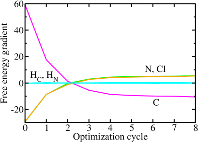
Figure 1: The $z$ component of approximate free energy gradient $\nabla A^{(n)}$ (in kcal/mol/Å) at $s=0.0$ Å  as a function of iterative optimization cycle $n$.

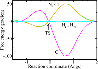
Figure 2: The $z$ components of free energy gradient $\nabla A^{\mathrm{MF}}(\mathbf{R}^{*}(s))$ (in kcal/mol/Å) as a function of reaction coordinate $s$ (in Å). The arrow indicates the location of the transition state in solution.

By integrating the gradients in Fig. 2, we obtain a free energy profile $A^{\mathrm{MF}}(s)\equiv A^{\mathrm{MF}}(\mathbf{R}^{*}(s))$ in Fig. 3 (solid line with circles). The barrier top of $A^{\mathrm{MF}}(s)$ is located at $s^{\ddagger}=-0.05$ Å, which corresponds to $r^{\ddagger}(\mathrm{C-N})=2.215$ Å  and $r^{\ddagger}(\mathrm{C-Cl})=2.165$ Å. The free energy of activation and of reaction are defined here as

$$\Delta A^{\ddagger} = A^{\mathrm{MF}}(s^{\ddagger})-A^{\mathrm{MF}}(s=-1.6),$$

$$\Delta A_{\mathrm{r}} = A^{\mathrm{MF}}(s=2.0)-A^{\mathrm{MF}}(s=-1.6),$$

which are found to be $\Delta A^{\ddagger}=10.6$ kcal/mol and $\Delta A_{\mathrm{r}}=-38.7$ kcal/mol at the BHHLYP/6-31+G(d,p) level. By adding solute entropic contributions,Truong et al. (1997); Amovilli et al. (1998) we obtain $\Delta G^{\ddagger}=\Delta A^{\ddagger}+13.1=23.7$ kcal/mol, which is in good agreement with $\Delta G^{\ddagger}=25.6$ kcal/mol obtained by Aguilar et al. at the BHHLYP/aug-cc-pVDZ level. Galvan et al. (2004) On the other hand, the reaction free energy is $\Delta G_{\mathrm{r}}=\Delta A_{\mathrm{r}}+7.5=-31.2$ kcal/mol, which falls within the error bar of the experimental result, $-34\pm 10$ kcal/mol.Gao and Xia (1993)

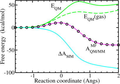
Figure 3: Free energy profile $A^{\mathrm{MF}}$ in Eq. (30) at the BHHLYP/6-31+G(d,p) level without solute entropic contributions (solid line with circles). The solid line and circles are obtained with Eqs. (54) and (55), respectively. $E_{\mathrm{QM}}$, $E_{\mathrm{QM}}(\mathrm{gas})$, and $\Delta A_{\mathrm{MM}}$ represent the internal QM energy in Eq. (26), its gas-phase counterpart, and the (relative) solvation free energy in Eq. (21), respectively. All the profiles are depicted such that they coincide at $s=-1.6$ Å.

Figure 3 also illustrates how the internal QM energy $E_{\mathrm{QM}}(\mathbf{R},\mathbf{v}^{\mathrm{sc}})$ and the (relative) solvation free energy $\Delta A_{\mathrm{MM}}(\mathbf{R},\mathbf{Q}^{\mathrm{sc}})$ vary as functions of $s$. The gas-phase counterpart of the former [i.e., $E_{\mathrm{QM}}(\mathbf{R},\mathbf{v}^{\prime}=\mathbf{0})$ along the gas-phase optimized path] is also plotted. To facilitate the comparison, all the profiles are shifted vertically such that they coincide at $s=-1.6$ Å. Figure 3 shows that $A^{\mathrm{MF}}$ is determined by strong cancellation between $E_{\mathrm{QM}}$ and $\Delta A_{\mathrm{MM}}$. While the QM electronic energy increases steeply with the separation of the ion pair, this is more than compensated by strong electrostatic stabilization by the solvent. Figures 4 and 5 illustrate how the QM fragment charges and MM mean potentials vary as functions of $s$. The optimized reaction paths in the gas phase and in solution are compared in Fig. 6. As stressed previously,Gao and Xia (1993) the transition state in solution [i.e., the saddle point of $A^{\mathrm{MF}}(\mathbf{R})$] is shifted remarkably toward the reactant region. This indicates that for the present charge separation reaction, the transition state in the gas phase should not be used for calculating the activation free energy in solution.

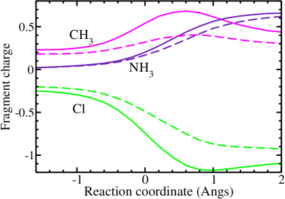
Figure 4: Fragment charges for $\mathrm{CH_{3}}$, $\mathrm{NH_{3}}$, and Cl atom in solution (solid lines) and in the gas phase (dashed lines).

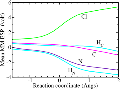
Figure 5: Mean electrostatic potentials $\mathbf{v}^{\mathrm{sc}}$ from the MM environment.

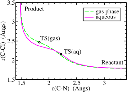
Figure 6: Reaction paths optimized in solution (solid line) and in the gas phase (dashed line). “TS(aq)” and “TS(gas)” represent the transition states corresponding to the top of the barrier of $A^{\mathrm{MF}}$ and $E_{\mathrm{QM}}(\mathrm{gas})$ in Fig. 3, respectively.

To check the validity of the free energy gradient, separate free-energy perturbation (FEP) calculations were also performed. Free energy differences between neighboring points of $s_{k}$ (corresponding to circles in Fig. 3) were calculated as

$$A^{\mathrm{MF}}(\mathbf{R}^{*}_{k+1})-A^{\mathrm{MF}}(\mathbf{R}^{*}_{k})\\ =-\frac{1}{\beta}\ln\ll\exp(-\beta\Delta E_{k+1,k})\gg_{k},$$ (60)

where $\mathbf{R}^{*}_{k}=\mathbf{R}^{*}(s_{k})$, $\Delta E_{k+1,k}=E^{\mathrm{MF}}(\mathbf{R}^{*}_{k+1},\mathbf{R}^{+})-E^{\mathrm{MF}}(\mathbf{R}^{*}_{k},\mathbf{R}^{+})$ with $E^{\mathrm{MF}}(\mathbf{R},\mathbf{R}^{+})$ given in Eq. (36), and $\ll\cdots\gg_{k}$ denotes the statistical average with the sampling function $\exp[-\beta E^{\mathrm{MF}}(\mathbf{R}^{*}_{k},\mathbf{R}^{+})]$. The necessary input like $\mathbf{R}^{*}_{k}$ was obtained from the TI calculation. Since FEP does not utilize the gradient information, the comparison of FEP profiles with TI ones offers a stringent test of consistency between $A^{\mathrm{MF}}(\mathbf{R})$ and $\nabla A^{\mathrm{MF}}(\mathbf{R})$. Figure 7 shows that the FEP profiles thus obtained are in excellent agreement with the TI ones, indicating that the free energy gradient is calculated correctly. Although there are slight differences between the FEP and TI profiles in the product region, this may be due to electrostatic finite-size effects,Not (b) because the agreement becomes better for a larger number of solvent molecules $N=997$ than $N=253$.

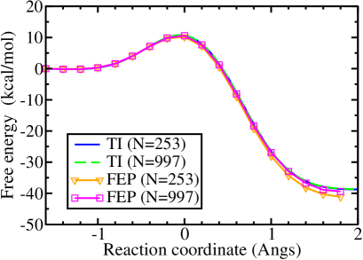
Figure 7: Free energy profiles obtained with thermodynamic integration (TI) and free energy perturbation (FEP). $N$ is the number of water solvent molecules.

Figure 8 compares the free energy profiles obtained at the HF, MP2, B3LYP, and BHHLYP levels with a larger basis set 6-311+G(2d,2p). This figure shows that the MP2 gives the highest value of the free energy barrier, $\Delta A^{\ddagger}=15.5$ kcal/mol, the B3LYP gives the lowest value, 9.2 kcal/mol, and the BHHLYP their intermediate, 11.9 kcal/mol (without including solute entropic contributions). Table 2 summarizes those values of $\Delta A^{\ddagger}$ and $\Delta A_{\mathrm{r}}$ obtained with various QM methods and basis sets. If we assume that the BHHLYP gives the “best” energetics for the present reaction,Truong et al. (1997) our main results are $\Delta G^{\ddagger}=11.9+13.1=25.0$ kcal/mol and $\Delta G_{\mathrm{r}}=-37.1+7.5=-29.6$ kcal/mol (including solute entropic contributions).

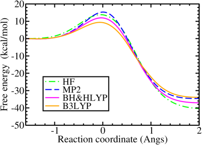
Figure 8: Free energy profiles obtained at the HF, MP2, B3LYP, and BHHLYP levels with the 6-311+G(2d,2p) basis set. The MP2 gives the highest value of $\Delta A^{\ddagger}$, while the B3LYP gives the lowest. See Table 2 for individual values of $\Delta A^{\ddagger}$ and $\Delta A_{\mathrm{r}}$. The profiles do not include solute entropic contributions. The RESP method is used for all calculations.

Table 2: Free energy of activation $\Delta A^{\ddagger}$ and reaction $\Delta A_{\mathrm{r}}$ (in kcal/mol) obtained at the HF, MP2, B3LYP, and BHHLYP levels with the 6-31+G(d,p) basis. Values in parentheses are obtained with the 6-311+G(2d,2p) basis. To compare with the previous studies, one needs to add solute entropic contributions to $\Delta A^{\ddagger}$ and $\Delta A_{\mathrm{r}}$ such that $\Delta G^{\ddagger}\simeq\Delta A^{\ddagger}+13.1$ and $\Delta G_{\mathrm{r}}\simeq\Delta A_{\mathrm{r}}+7.5$ kcal/mol (Refs. Truong et al., 1997 and Amovilli et al., 1998). The RESP method is used for all calculations unless otherwise noted.

Method	$\Delta A^{\ddagger}$	$\Delta A_{\mathrm{r}}$
HF	12.0 (13.7)	$-41.6$ ($-40.4$)
MP2	16.8 (15.5)	$-35.1$ ($-34.6$)
B3LYP	7.8 (9.2)	$-36.9$ ($-33.9$)
BHHLYP	10.6 (11.9)	$-38.7$ ($-37.1$)
BHHLYP	10.6 (11.9)	$-38.7$ ($-34.0$)

To estimate the non-mean-field effects on QM/MM free energy, Table 3 lists the values of $\Delta A_{\mathrm{fluc}}$ evaluated using the Gaussian fluctuation model in Eq. (51). This table also gives the values of $\Delta E_{\mathrm{fluc}}$ defined by

$$\Delta E_{\mathrm{fluc}}=\ll\mathcal{E}_{\mathrm{QM}}(\mathbf{R},\mathbf{v}_{\mathrm{MM}})\gg_{\mathbf{Q}^{\mathrm{sc}}}-\mathcal{E}_{\mathrm{QM}}(\mathbf{R},\mathbf{v}^{\mathrm{sc}}),$$ (61)

which was also calculated using the Gaussian model as

$$\Delta E_{\mathrm{fluc}}\simeq\frac{1}{2}\mathrm{tr}[\boldsymbol{\chi}_{\mathrm{QM}}\boldsymbol{\sigma}_{\mathrm{MM}}].$$ (62)

This quantity was used previously by Naka et al.Naka et al. (1999a) and Aguilar et al.Sanchez et al. (2002) in order to study fluctuations of the QM wavefunction in solution. The table shows that the absolute values of $\Delta A_{\mathrm{fluc}}$ and $\Delta E_{\mathrm{fluc}}$ are considerably small ($<0.5$ kcal/mol) for the entire region of the reaction coordinate. They are also similar to the values reported for other organic molecules in water ($\Delta E_{\mathrm{fluc}}=-0.2\sim-0.5$ kcal/mol). Naka et al. (1999b); Sanchez et al. (2002) It should be noted that the impact of $\Delta A_{\mathrm{fluc}}(\mathbf{R})$ on free energy profiles is even smaller, because the variation of $\Delta A_{\mathrm{fluc}}(\mathbf{R}^{*}(s))$ as a function of $s$ is on the order of 0.1 kcal/mol. This result suggests that the non-mean-field effects on QM/MM free energy are rather small for the present reaction in water. Similar observations have been made in the literature. Sanchez et al. (2002); Galvan et al. (2006); Kastner et al. (2006); Takahashi et al. (2003) Nevertheless, we stress that it is not clear at present to what extent this conclusion applies to different types of systems, e.g., enzyme reactions where local fluctuations of the MM environment may deviate significantly from the Gaussian distribution.Simonson (2002)

Table 3: Fluctuation corrections for the free energy $\Delta A_{\mathrm{fluc}}$ in Eq. (51) and for the interaction energy $\Delta E_{\mathrm{fluc}}$ in Eq. (62) calculated with the BHHLYP/6-31+G(d,p) method. Values in parentheses are obtained with the 6-311+G(2d,2p) basis. RC stands for the reaction coordinate in Eq. (53). All energies are given in kcal/mol.

RC  (Å)	$\Delta A_{\mathrm{fluc}}$	$\Delta E_{\mathrm{fluc}}$
$-1.6$	$-0.43$ ($-0.44$)	$-0.38$ ($-0.39$)
$0.0$	$-0.41$ ($-0.45$)	$-0.36$ ($-0.40$)
$2.0$	$-0.30$ ($-0.34$)	$-0.28$ ($-0.31$)

IV Discussions and conclusions

Numerical stability of the ESP charge operator. ESP charges and associated charge operator $\hat{\mathbf{Q}}$ are sometimes numerically unstable, as often stressed in the literature.Hu et al. (2007b); Yokogawa et al. (2007); Ishida and Morita (2006) For example, we observed an oscillatory behavior of partial charges within the CH₃ group during the optimization cycles. This was typical for $s=0.8$ Å, where the ion pair products start to form. Since these oscillations are partly due to ambiguous assignment of partial charges for “buried” atoms, Ishida and Morita (2006) the RESP methodBayly et al. (1993) was of great help in suppressing those oscillations. However, the RESP method was of little help in removing a divergent behavior of partial charges within the NH₃ group observed in the reactant asymptotic region ($s<-2.0$ Å). Specifically, the partial charge on the N (H_N) atom kept on growing in the negative (positive) direction during the optimization cycles. This might be due to inherent limitations of the present charge model, where partial charges are placed only on atomic nuclei and the lone pair on the N atom may be poorly described. Galvan et al. (2006) In this respect, it may be more straightforward to use the continuous or mixed representation in Appendix A or D, where one embeds the MM point charges directly into the QM Hamiltonian. See Refs. Galvan et al., 2003a and Hu et al., 2008 for this type of implementation.

FEP that connects optimized geometries. If one is interested only in the free energy difference between two stationary points (e.g., activation free energy), it is probably more efficient to use FEP than TI. Specifically, one first searches the free energy surface for stationary points by using the free energy gradient (and possibly the hessian), and then connects these points via FEP. The QM geometries and charges of intermediate points could be generated by linear interpolation of two end points. See LABEL:Aguilar_ASEP_Mensh for such a calculation. In this way, one can reduce the number of costly free energy optimization. If one also needs to know a rough free energy profile, one could perform additional optimization for a limited number of intermediate points and then connect them via FEP.

Solute thermal/entropic contributions. The method in this paper calculates the QM/MM free energy for a given fixed QM geometry. The thermal/entropic contributions of the QM subsystem thus need to be taken into account separately, e.g., via harmonic vibration approximations. This is a well-known limitation of the present type of method, which is also shared by conventional solvation theories. To overcome this limitation, several methods have been proposed for a priori including the solute flexibility into the QM/MM free energy calculation at a reasonable computational cost. Rosta et al. (2006); Lu and Yang (2004); Higashi and Truhlar (2008)

To conclude, we have presented a direct QM/MM analog of conventional solvation theories based on variational and perturbative frameworks. The main approximation in this paper is that the true QM wavefunction is replaced by an averaged one that is calculated in the MM mean field. We stress however that the electrostatic interactions between the averaged QM wavefunction and the MM environment are calculated correctly without further approximations. The basic appeal of the mean-field QM/MM approach is that it can describe different environments (e.g., solutions and enzymes) on an equal theoretical footing, while the number of QM calculations can be made significantly smaller than a direct QM/MM calculation.

Appendix A Continuous representation

The main text is based on the approximate Schrödinger equation in Eq. (7), where QM/MM electrostatic interactions are “discretized” in terms of the ESP charge operator. In this section we summarize an alternative formulation using the continuous Schrödinger equation in Eq. (5).

First, the total energy is given by

$$E(\mathbf{R},\mathbf{R}^{+})=\mathcal{E}_{\mathrm{QM}}[\mathbf{R},v_{\mathrm{MM}}]+\mathcal{E}_{\mathrm{MM}}(\mathbf{R},\mathbf{R}^{+}),$$ (63)

where $\mathcal{E}_{\mathrm{QM}}[\mathbf{R},v_{\mathrm{MM}}]$ is defined via Eq. (5) with $v^{\prime}(\mathbf{x})=v_{\mathrm{MM}}(\mathbf{x},\mathbf{R}^{+})$. We then expand $\mathcal{E}_{\mathrm{QM}}[\mathbf{R},v_{\mathrm{MM}}]$ in terms of $v_{\mathrm{MM}}(\mathbf{x},\mathbf{R}^{+})$ up to first order,

$$\mathcal{E}_{\mathrm{QM}}[\mathbf{R},v_{\mathrm{MM}}] \simeq \mathcal{E}_{\mathrm{QM}}[\mathbf{R},v^{\mathrm{sc}}]+\int d\mathbf{x}\rho^{\mathrm{sc}}(\mathbf{x}|\mathbf{R})\{v_{\mathrm{MM}}(\mathbf{x},\mathbf{R}^{+})-v^{\mathrm{sc}}(\mathbf{x}|\mathbf{R})\}$$ (64)

$$= E_{\mathrm{QM}}[\mathbf{R},v^{\mathrm{sc}}]+\int d\mathbf{x}\rho^{\mathrm{sc}}(\mathbf{x}|\mathbf{R})v_{\mathrm{MM}}(\mathbf{x},\mathbf{R}^{+}),$$

where $E_{\mathrm{QM}}[\mathbf{R},v^{\mathrm{sc}}]=\langle\Psi^{\mathrm{sc}}|\hat{H}_{\mathrm{QM}}|\Psi^{\mathrm{sc}}\rangle$ and we have used the following Hellmann-Feynman theorem:

$$\frac{\delta\mathcal{E}_{\mathrm{QM}}[\mathbf{R},v^{\prime}]}{\delta v^{\prime}(\mathbf{x})}=\langle\Psi[\mathbf{R},v^{\prime}]|\hat{\rho}(\mathbf{x})|\Psi[\mathbf{R},v^{\prime}]\rangle.$$ (65)

$\rho^{\mathrm{sc}}(\mathbf{x}|\mathbf{R})$ and $v^{\mathrm{sc}}(\mathbf{x}|\mathbf{R})$ are obtained from the following self-consistency condition,

$$v^{\mathrm{sc}}(\mathbf{x}|\mathbf{R})=\ll v_{\mathrm{MM}}(\mathbf{x},\mathbf{R}^{+})\gg_{\rho^{\mathrm{sc}}},$$ (66a)

$$\rho^{\mathrm{sc}}(\mathbf{x}|\mathbf{R})=\langle\Psi^{\mathrm{sc}}|\hat{\rho}(\mathbf{x})|\Psi^{\mathrm{sc}}\rangle,$$ (66b)

with $\Psi^{\mathrm{sc}}\equiv\Psi[\mathbf{R},v^{\mathrm{sc}}]$. Note that $v^{\mathrm{sc}}$ and $\rho^{\mathrm{sc}}$ depend parametrically on $\mathbf{R}$ via Eq. (66). $\ll\cdots\gg$ is the statistical average defined by

$$\ll\cdots\gg_{\rho^{\prime}}=\frac{\int d\mathbf{R}^{+}e^{-\beta\mathcal{E}[\rho^{\prime},\mathbf{R},\mathbf{R}^{+}]}(\cdots)}{\int d\mathbf{R}^{+}e^{-\beta\mathcal{E}[\rho^{\prime},\mathbf{R},\mathbf{R}^{+}]}},$$ (67)

with

$$\mathcal{E}[\rho^{\prime},\mathbf{R},\mathbf{R}^{+}]=\int d\mathbf{x}\rho^{\prime}(\mathbf{x})v_{\mathrm{MM}}(\mathbf{x},\mathbf{R}^{+})+\mathcal{E}_{\mathrm{MM}}(\mathbf{R},\mathbf{R}^{+}).$$ (68)

Inserting the above first-order expansion into $A(\mathbf{R})$ in Eq. (3) gives the QM/MM free energy with mean-field embedding,

$$A^{\mathrm{MF}}(\mathbf{R})=E_{\mathrm{QM}}[\mathbf{R},v^{\mathrm{sc}}]+\Delta A_{\mathrm{MM}}[\mathbf{R},\rho^{\mathrm{sc}}],$$ (69)

with

$$\Delta A_{\mathrm{MM}}[\mathbf{R},\rho^{\prime}]=-\frac{1}{\beta}\ln\int d\mathbf{R}^{+}e^{-\beta\mathcal{E}[\rho^{\prime},\mathbf{R},\mathbf{R}^{+}]}.$$ (70)

The gradient of $A^{\mathrm{MF}}(\mathbf{R})$ can be obtained via similar arguments as

$$\frac{\partial}{\partial\mathbf{R}}A^{\mathrm{MF}}(\mathbf{R})=\left.\frac{\partial\mathcal{E}_{\mathrm{QM}}[\mathbf{R},v^{\prime}]}{\partial\mathbf{R}}\right|_{v^{\prime}=v^{\mathrm{sc}}}+\left.\frac{\partial\Delta A_{\mathrm{MM}}[\mathbf{R},\rho^{\prime}]}{\partial\mathbf{R}}\right|_{\rho^{\prime}=\rho^{\mathrm{sc}}}.$$ (71)

The first term represents the energy gradient in a fixed external field. The second term may be rewritten using Eq. (70) as

$$\left.\frac{\partial\Delta A_{\mathrm{MM}}[\mathbf{R},\rho^{\prime}]}{\partial\mathbf{R}}\right|_{\rho^{\prime}=\rho^{\mathrm{sc}}}=\;\ll\frac{\partial\mathcal{E}_{\mathrm{MM}}(\mathbf{R},\mathbf{R}^{+})}{\partial\mathbf{R}}\gg_{\rho^{\mathrm{sc}}}.$$ (72)

Note that the above equation lacks the electrostatic term like $Q^{\mathrm{sc}}_{a}\ll\partial v_{\mathrm{MM},a}/\partial\mathbf{R}_{a}\gg$ that is present in the the discretized case [Eq. (35)]. This discrepancy originates from the different physical meaning of $\partial\mathcal{E}_{\mathrm{QM}}[\mathbf{R},v^{\prime}]/\partial\mathbf{R}$ (in the continuous representation) and $\partial\mathcal{E}_{\mathrm{QM}}(\mathbf{R},\mathbf{v}^{\prime})/\partial\mathbf{R}$ (in the discretized representation). In the discretized case, the external potential values $\mathbf{v}^{\prime}$ acting on QM atoms are kept constant while varying the nuclear coordinates $\mathbf{R}$. In the continuous case, the external potential field $v^{\prime}(\mathbf{x})$ is kept constant while varying $\mathbf{R}$. This means that the potential values acting on QM atoms, $v^{\prime}(\mathbf{R}_{a})$, may vary as a function of $\mathbf{R}$. The situation becomes clear by considering the following relation:

$$\left.\frac{\partial\mathcal{E}_{\mathrm{QM}}[\mathbf{R},v^{\prime}]}{\partial\mathbf{R}_{a}}\right|_{v^{\prime}=v^{\mathrm{sc}}} \simeq \left.\frac{\partial}{\partial\mathbf{R}_{a}}\mathcal{E}_{\mathrm{QM}}(\mathbf{R},\{v^{\mathrm{sc}}(\mathbf{R}_{b}|\mathbf{X})\})\right|_{\mathbf{X}=\mathbf{R}}$$

$$\simeq \left.\frac{\partial\mathcal{E}_{\mathrm{QM}}(\mathbf{R},\mathbf{v}^{\prime})}{\partial\mathbf{R}_{a}}\right|_{\mathbf{v}^{\prime}=\mathbf{v}^{\mathrm{sc}}}$$

$$+ Q^{\mathrm{sc}}_{a}(\mathbf{R})\ll\frac{\partial v_{\mathrm{MM}}(\mathbf{R}_{a},\mathbf{R}^{+})}{\partial\mathbf{R}_{a}}\gg_{\mathbf{Q}^{\mathrm{sc}}},$$

where we have used the following identity obtained from Eq. (66a):

$$\left.\frac{\partial v^{\mathrm{sc}}(\mathbf{R}_{a}|\mathbf{X})}{\partial\mathbf{R}_{a}}\right|_{\mathbf{X}=\mathbf{R}} = \left.\frac{\partial v^{\mathrm{sc}}(\mathbf{x}|\mathbf{R})}{\partial\mathbf{x}}\right|_{\mathbf{x}=\mathbf{R}_{a}}$$

$$= \left.\ll\frac{\partial v_{\mathrm{MM}}(\mathbf{x},\mathbf{R}^{+})}{\partial\mathbf{x}}\gg_{\rho^{\mathrm{sc}}}\right|_{\mathbf{x}=\mathbf{R}_{a}}.$$

Therefore, it follows that the missing electrostatic term in Eq. (72) is now accounted for by the energy gradient term in Eq. (71).

Appendix B ESP charge operator

The ESP charges $\{Q_{a}\}$ for a given wavefunction $\Psi$ are obtained by minimizing the following functionBayly et al. (1993)

$$L(\mathbf{Q},\lambda) = \sum_{l}^{\mathrm{grid}}\left\{\int d\mathbf{x}\frac{\langle\Psi|\hat{\rho}(\mathbf{x})|\Psi\rangle}{|\mathbf{G}_{l}-\mathbf{x}|}-\sum_{a}\frac{Q_{a}}{|\mathbf{G}_{l}-\mathbf{R}_{a}|}\right\}^{2}$$ (75)

$$-\lambda\left[\sum_{a}Q_{a}-Q_{\mathrm{tot}}\right],$$

where $\{\mathbf{G}_{l}\}$ are the ESP fitting grid and $Q_{\mathrm{tot}}$ is the total charge. By requiring that $\partial L(\mathbf{Q},\lambda)/\partial\mathbf{Q}=0$, inverting the resulting linear equations for $\mathbf{Q}$, and determining $\lambda$ via $\sum_{a}Q_{a}=Q_{\mathrm{tot}}$, we obtain

$$Q_{a}=\langle\Psi|\hat{Q}_{a}|\Psi\rangle,$$ (76)

where $\hat{Q}_{a}$ is an explicit function of $\{\mathbf{r}_{i}\},\{\mathbf{R}_{a}\},\{\mathbf{G}_{k}\},$ and $Q_{\mathrm{tot}}$, with $\{\mathbf{r}_{i}\}$ being the electron coordinates. See previous work for the explicit form of $\hat{Q}_{a}$ in the atomic orbital basis. Ten-no et al. (1994); Sato et al. (1996); Morita and Kato (1997, 1998); Ishida and Morita (2006) The above definition of $\hat{\mathbf{Q}}$ suggests that one may make the following replacement

$$\int d\mathbf{x}\frac{\hat{\rho}(\mathbf{x})}{|\mathbf{y}-\mathbf{x}|}\simeq\sum_{a}\frac{\hat{Q}_{a}}{|\mathbf{y}-\mathbf{R}_{a}|},$$ (77)

as long as $\mathbf{y}$ is located outside the core region of the QM charge density. Then, the continuous QM/MM electrostatic interaction may be discretized as

$$\int d\mathbf{x}\hat{\rho}(\mathbf{x})v_{\mathrm{MM}}(\mathbf{x},\mathbf{R}^{+})\simeq\sum_{a}\hat{Q}_{a}v_{\mathrm{MM}}(\mathbf{R}_{a},\mathbf{R}^{+}),$$ (78)

by inserting the definition of $v_{\mathrm{MM}}(\mathbf{x},\mathbf{R}^{+})$ in Eq. (9). This is the present rationale for using $\hat{\mathbf{Q}}$ in Eq. (7).

Appendix C Comparison with the QM/MM-MFEP method

Here we compare the perturbative treatment of $A^{\mathrm{MF}}(\mathbf{R})$ in Sec. II.3 with the QM/MM-MFEP method. Hu et al. (2007a, 2008) The starting point is the same as Eq. (3) (here expressed using the notation in LABEL:Yang_QMMM_MFEP08),

$$A(\mathbf{r}_{\mathrm{QM}})=-\frac{1}{\beta}\ln\int d\mathbf{r}_{\mathrm{MM}}\exp\{-\beta E(\mathbf{r}_{\mathrm{QM}},\mathbf{r}_{\mathrm{MM}})\},$$ (79)

where $\mathbf{r}_{\mathrm{QM}}=\mathbf{R}$, $\mathbf{r}_{\mathrm{MM}}=\mathbf{R}^{+}$, and the total energy is given by

$$E(\mathbf{r}_{\mathrm{QM}},\mathbf{r}_{\mathrm{MM}})=\langle\Psi|\hat{H}_{\mathrm{eff}}|\Psi\rangle+\mathcal{E}_{\mathrm{MM}}(\mathbf{r}_{\mathrm{QM}},\mathbf{r}_{\mathrm{MM}}).$$ (80)

$\hat{H}_{\mathrm{eff}}$ is the effective QM Hamiltonian in the presence of the MM electrostatic field,

$$\hat{H}_{\mathrm{eff}}=\hat{H}_{\mathrm{QM}}+\int d\mathbf{x}\hat{\rho}(\mathbf{x})v_{\mathrm{MM}}(\mathbf{x},\mathbf{r}_{\mathrm{MM}}),$$ (81)

and other quantities like $\hat{H}_{\mathrm{QM}}$ are defined in the main text. We then introduce the MM mean field as

$$v_{\mathrm{MM}}^{\circ}(\mathbf{x})=\frac{1}{L}\sum_{\tau=1}^{L}v_{\mathrm{MM}}(\mathbf{x},\mathbf{r}_{\mathrm{MM}}^{\circ}(\tau)),$$ (82)

where $\{\mathbf{r}_{\mathrm{MM}}^{\circ}(\tau)\}_{\tau=1}^{L}$ are a set of MM configurations obtained from the previous cycle of the sequential sampling/optimization method.Hu et al. (2008) The QM Hamiltonian in the presence of the MM mean field is defined by

$$\hat{H}_{\mathrm{eff}}^{\circ}=\hat{H}_{\mathrm{QM}}+\int d\mathbf{x}\hat{\rho}(\mathbf{x})v_{\mathrm{MM}}^{\circ}(\mathbf{x}).$$ (83)

The eigenfunction and eigenenergy of $\hat{H}_{\mathrm{eff}}^{\circ}$ are denoted as $|\Psi^{\circ}\rangle$ and $\langle\Psi^{\circ}|\hat{H}_{\mathrm{eff}}^{\circ}|\Psi^{\circ}\rangle\equiv\langle\Psi|\hat{H}_{\mathrm{eff}}|\Psi\rangle^{\circ}$, and the ESP charges derived from $|\Psi^{\circ}\rangle$ are written as $Q^{\circ}_{i}(\mathbf{r}_{\mathrm{QM}})$. The internal QM energy associated with $\hat{H}_{\mathrm{eff}}^{\circ}$ is defined as

$$E_{1}^{\circ}(\mathbf{r}_{\mathrm{QM}})\equiv\langle\Psi|\hat{H}_{\mathrm{eff}}|\Psi\rangle^{\circ}-\sum_{i}^{\mathrm{QM}}Q^{\circ}_{i}(\mathbf{r}_{\mathrm{QM}})v_{\mathrm{MM}}^{\circ}(\mathbf{r}_{\mathrm{QM},i}),$$ (84)

i.e., by subtracting the QM/MM electrostatic interaction energy expressed in terms of ESP charges from the effective QM energy.

The QM/MM-MFEP method then develops a series of polarizable QM models by Taylor expanding its energy and ESP charges up to first or second order. Among others, Model 3 (“QM point charges with polarization due to MM and QM atoms”) approximates the total energy as follows [Eqs. (36) and (40) of LABEL:Yang_QMMM_MFEP08]:

$$\tilde{E}(\mathbf{r}_{\mathrm{QM}},\mathbf{r}_{\mathrm{MM}}) = E_{1}^{\circ}(\mathbf{r}_{\mathrm{QM}})$$

$$+ \sum_{i}^{\mathrm{QM}}Q^{\circ}_{i}(\mathbf{r}_{\mathrm{QM}})v_{\mathrm{MM}}(\mathbf{r}_{\mathrm{QM},i},\mathbf{r}_{\mathrm{MM}})$$

$$+ \frac{1}{2}\sum_{i}^{\mathrm{QM}}\sum_{j}^{\mathrm{QM}}[v_{\mathrm{MM}}(\mathbf{r}_{\mathrm{QM},i},\mathbf{r}_{\mathrm{MM}})-v_{\mathrm{MM}}^{\circ}(\mathbf{r}_{\mathrm{QM},i})]$$

$$\times\chi_{ij}[v_{\mathrm{MM}}(\mathbf{r}_{\mathrm{QM},j},\mathbf{r}_{\mathrm{MM}})-v_{\mathrm{MM}}^{\circ}(\mathbf{r}_{\mathrm{QM},j})]$$

$$+ \mathcal{E}_{\mathrm{MM}}(\mathbf{r}_{\mathrm{QM}},\mathbf{r}_{\mathrm{MM}}),$$

where $\chi_{ij}$ is the charge response kernel in Eq. (48). The above equation may be viewed as the second-order expansion of the effective QM energy in terms of MM electrostatic potential [cf. Eq. (47)]. The gradient of QM/MM free energy is obtained by inserting Eq. (C) into the following,

$$\frac{\partial A(\mathbf{r}_{\mathrm{QM}})}{\partial\mathbf{r}_{\mathrm{QM}}}\simeq\left\langle\frac{\partial\tilde{E}(\mathbf{r}_{\mathrm{QM}},\mathbf{r}_{\mathrm{MM}})}{\partial\mathbf{r}_{\mathrm{QM}}}\right\rangle_{\tilde{E}},$$ (86)

or alternately, into an FEP-type expression [Eq. (6) of LABEL:Yang_QMMM_MFEP08]

$$\frac{\partial A(\mathbf{r}_{\mathrm{QM}})}{\partial\mathbf{r}_{\mathrm{QM}}}\simeq\frac{\left\langle\frac{\partial\tilde{E}(\mathbf{r}_{\mathrm{QM}},\mathbf{r}_{\mathrm{MM}})}{\partial\mathbf{r}_{\mathrm{QM}}}e^{-\beta(\tilde{E}(\mathbf{r}_{\mathrm{QM}},\mathbf{r}_{\mathrm{MM}})-E_{\mathrm{ref}}(\mathbf{r}_{\mathrm{MM}}))}\right\rangle_{E_{\mathrm{ref}}}}{\left\langle e^{-\beta(\tilde{E}(\mathbf{r}_{\mathrm{QM}},\mathbf{r}_{\mathrm{MM}})-E_{\mathrm{ref}}(\mathbf{r}_{\mathrm{MM}}))}\right\rangle_{E_{\mathrm{ref}}}},$$ (87)

where $E_{\mathrm{ref}}(\mathbf{r}_{\mathrm{MM}})$ is the reference sampling function that is obtained from the previous cycle of the sequential sampling/optimization method.Hu et al. (2008)

The main difference of the present approach from the QM/MM-MFEP method is that the present one utilizes the self-consistency condition in order to simplify the gradient expression. To see this, let us insert $\tilde{E}(\mathbf{r}_{\mathrm{QM}},\mathbf{r}_{\mathrm{MM}})$ in Eq. (C) into the statistical average in Eq. (86),

$$\frac{\partial A(\mathbf{r}_{\mathrm{QM}})}{\partial\mathbf{r}_{\mathrm{QM}}} = \frac{\partial E_{1}^{\circ}(\mathbf{r}_{\mathrm{QM}})}{\partial\mathbf{r}_{\mathrm{QM}}}$$ (88)

$$+\sum_{i}^{\mathrm{QM}}\frac{\partial Q^{\circ}_{i}(\mathbf{r}_{\mathrm{QM}})}{\partial\mathbf{r}_{\mathrm{QM}}}\langle v_{\mathrm{MM}}(\mathbf{r}_{\mathrm{QM},i},\mathbf{r}_{\mathrm{MM}})\rangle_{\tilde{E}}$$

$$+\sum_{i}^{\mathrm{QM}}Q^{\circ}_{i}(\mathbf{r}_{\mathrm{QM}})\left\langle\frac{\partial v_{\mathrm{MM}}(\mathbf{r}_{\mathrm{QM},i},\mathbf{r}_{\mathrm{MM}})}{\partial\mathbf{r}_{\mathrm{QM}}}\right\rangle_{\tilde{E}}$$

$$+\left\langle\frac{\partial\mathcal{E}_{\mathrm{MM}}(\mathbf{r}_{\mathrm{QM}},\mathbf{r}_{\mathrm{MM}})}{\partial\mathbf{r}_{\mathrm{QM}}}\right\rangle_{\tilde{E}},$$

where terms depending on $\chi_{ij}$ have been neglected (they are treated separately in Sec. II.4). Using Eq. (84), we may rewrite the above equation as

$$\frac{\partial A(\mathbf{r}_{\mathrm{QM}})}{\partial\mathbf{r}_{\mathrm{QM}}} = \frac{\partial\langle\Psi|\hat{H}_{\mathrm{eff}}|\Psi\rangle^{\circ}}{\partial\mathbf{r}_{\mathrm{QM}}}+\sum_{i}^{\mathrm{QM}}\frac{\partial Q^{\circ}_{i}(\mathbf{r}_{\mathrm{QM}})}{\partial\mathbf{r}_{\mathrm{QM}}}\left\{\langle v_{\mathrm{MM}}(\mathbf{r}_{\mathrm{QM},i},\mathbf{r}_{\mathrm{MM}})\rangle_{\tilde{E}}-v_{\mathrm{MM}}^{\circ}(\mathbf{r}_{\mathrm{QM},i})\right\}$$ (89)

$$+\sum_{i}^{\mathrm{QM}}Q^{\circ}_{i}(\mathbf{r}_{\mathrm{QM}})\left\{\left\langle\frac{\partial v_{\mathrm{MM}}(\mathbf{r}_{\mathrm{QM},i},\mathbf{r}_{\mathrm{MM}})}{\partial\mathbf{r}_{\mathrm{QM}}}\right\rangle_{\tilde{E}}-\frac{\partial v_{\mathrm{MM}}^{\circ}(\mathbf{r}_{\mathrm{QM},i})}{\partial\mathbf{r}_{\mathrm{QM}}}\right\}+\left\langle\frac{\partial\mathcal{E}_{\mathrm{MM}}(\mathbf{r}_{\mathrm{QM}},\mathbf{r}_{\mathrm{MM}})}{\partial\mathbf{r}_{\mathrm{QM}}}\right\rangle_{\tilde{E}}.$$

Now let us assume that the reference MM coordinates $\{\mathbf{r}_{\mathrm{MM}}^{\circ}(\tau)\}$ satisfies the following self-consistency condition

$$\langle f(\mathbf{r}_{\mathrm{QM}},\mathbf{r}_{\mathrm{MM}})\rangle_{\tilde{E}}\simeq\frac{1}{L}\sum_{\tau=1}^{L}f(\mathbf{r}_{\mathrm{QM}},\mathbf{r}_{\mathrm{MM}}^{\circ}(\tau)),\;\;\;\forall f,$$ (90)

which is expected to hold well for the last few cycles of the sequential sampling/optimization method.Hu et al. (2008)Then, by setting $f=v_{\mathrm{MM}}(\mathbf{r}_{\mathrm{QM},i},\mathbf{r}_{\mathrm{MM}})$ or $f=\partial v_{\mathrm{MM}}(\mathbf{r}_{\mathrm{QM},i},\mathbf{r}_{\mathrm{MM}})/\partial\mathbf{r}_{\mathrm{QM}}$, we have

$$\langle v_{\mathrm{MM}}(\mathbf{r}_{\mathrm{QM},i},\mathbf{r}_{\mathrm{MM}})\rangle_{\tilde{E}} \simeq \frac{1}{L}\sum_{\tau=1}^{L}v_{\mathrm{MM}}(\mathbf{r}_{\mathrm{QM},i},\mathbf{r}_{\mathrm{MM}}^{\circ}(\tau))$$ (91a)

$$= v_{\mathrm{MM}}^{\circ}(\mathbf{r}_{\mathrm{QM},i}),$$

$$\left\langle\frac{\partial v_{\mathrm{MM}}(\mathbf{r}_{\mathrm{QM},i},\mathbf{r}_{\mathrm{MM}})}{\partial\mathbf{r}_{\mathrm{QM}}}\right\rangle_{\tilde{E}} \simeq \frac{1}{L}\sum_{\tau=1}^{L}\frac{\partial v_{\mathrm{MM}}(\mathbf{r}_{\mathrm{QM},i},\mathbf{r}_{\mathrm{MM}}^{\circ}(\tau))}{\partial\mathbf{r}_{\mathrm{QM}}}$$ (91b)

$$= \frac{\partial v_{\mathrm{MM}}^{\circ}(\mathbf{r}_{\mathrm{QM},i})}{\partial\mathbf{r}_{\mathrm{QM}}},$$

which suggest that the curly brackets in Eq. (89) vanish, and as a result we obtain a simpler expression for the free energy gradient,

$$\frac{\partial A(\mathbf{r}_{\mathrm{QM}})}{\partial\mathbf{r}_{\mathrm{QM}}}\simeq\frac{\partial\langle\Psi|\hat{H}_{\mathrm{eff}}|\Psi\rangle^{\circ}}{\partial\mathbf{r}_{\mathrm{QM}}}+\left\langle\frac{\partial\mathcal{E}_{\mathrm{MM}}(\mathbf{r}_{\mathrm{QM}},\mathbf{r}_{\mathrm{MM}})}{\partial\mathbf{r}_{\mathrm{QM}}}\right\rangle_{\tilde{E}}.$$ (92)

This form is found to be equivalent with the present gradient expressions, e.g., Eq. (71).

Appendix D Mixed representation

As seen from Eqs. (84) and (C), the QM/MM-MFEP method is based on a “mixed” representation of the QM/MM electrostatic interactions. That is, the QM wavefunction is calculated with the continuous Schrödinger equation in Eq. (5), while the internal QM energy etc are defined in terms of ESP charges. In this mixed representation, $A^{\mathrm{MF}}(\mathbf{R})$ may be defined as

$$A^{\mathrm{MF}}(\mathbf{R}) = \mathcal{E}_{\mathrm{QM}}[\mathbf{R},v^{\mathrm{sc}}]-\sum_{a}Q^{\mathrm{sc}}_{a}(\mathbf{R})v^{\mathrm{sc}}(\mathbf{R}_{a}|\mathbf{R})$$ (93)

$$+\Delta A_{\mathrm{MM}}(\mathbf{R},\mathbf{Q}^{\mathrm{sc}}),$$

and the mixed form of the self-consistency condition is

$$v^{\mathrm{sc}}(\mathbf{x}|\mathbf{R}) = \ll v_{\mathrm{MM}}(\mathbf{x},\mathbf{R}^{+})\gg_{\mathbf{Q}^{\mathrm{sc}}},$$ (94a)

$$Q^{\mathrm{sc}}_{a}(\mathbf{R}) = \langle\Psi^{\mathrm{sc}}|\hat{Q}_{a}|\Psi^{\mathrm{sc}}\rangle,$$ (94b)

where $\Psi^{\mathrm{sc}}=\Psi[\mathbf{R},v^{\mathrm{sc}}]$. The gradient of $A^{\mathrm{MF}}(\mathbf{R})$ then becomes

$$\frac{\partial}{\partial\mathbf{R}_{a}}A^{\mathrm{MF}}(\mathbf{R}) = \left.\frac{\mathcal{E}_{\mathrm{QM}}[\mathbf{R},v^{\prime}]}{\partial\mathbf{R}_{a}}\right|_{v^{\prime}=v^{\mathrm{sc}}}+\sum_{b}\frac{\partial Q^{\mathrm{sc}}_{b}(\mathbf{R})}{\partial\mathbf{R}_{a}}\left\{\ll v_{\mathrm{MM}}(\mathbf{R}_{b},\mathbf{R}^{+})\gg_{\mathbf{Q}^{\mathrm{sc}}}-v^{\mathrm{sc}}(\mathbf{R}_{b}|\mathbf{R})\right\}$$ (95)

$$+Q^{\mathrm{sc}}_{a}(\mathbf{R})\left\{\ll\frac{\partial v_{\mathrm{MM}}(\mathbf{R}_{a},\mathbf{R}^{+})}{\partial\mathbf{R}_{a}}\gg_{\mathbf{Q}^{\mathrm{sc}}}-\left.\frac{\partial v^{\mathrm{sc}}(\mathbf{R}_{a}|\mathbf{X})}{\partial\mathbf{R}_{a}}\right|_{\mathbf{X}=\mathbf{R}}\right\}+\ll\frac{\partial\mathcal{E}_{\mathrm{MM}}(\mathbf{R},\mathbf{R}^{+})}{\partial\mathbf{R}_{a}}\gg_{\mathbf{Q}^{\mathrm{sc}}}$$

$$+\int d\mathbf{x}\rho^{\mathrm{sc}}(\mathbf{x}|\mathbf{R})\frac{\partial v^{\mathrm{sc}}(\mathbf{x}|\mathbf{R})}{\partial\mathbf{R}_{a}}-\sum_{b}Q^{\mathrm{sc}}_{b}(\mathbf{R})\left[\frac{\partial v^{\mathrm{sc}}(\mathbf{x}|\mathbf{R})}{\partial\mathbf{R}_{a}}\right]_{\mathbf{x}=\mathbf{R}_{b}},$$

where $\rho^{\mathrm{sc}}(\mathbf{x}|\mathbf{R})\equiv\langle\Psi^{\mathrm{sc}}|\hat{\rho}(\mathbf{x})|\Psi^{\mathrm{sc}}\rangle$. The curly brackets in the above equation vanish by using Eq. (94a) and its derivative with respect to $\mathbf{x}$ [see also Eq. (A)]. The third line also vanishes approximately since $\mathbf{Q}^{\mathrm{sc}}$ represent the ESP charges that correspond to $\rho^{\mathrm{sc}}$. Therefore, we obtain the following gradient:

$$\frac{\partial}{\partial\mathbf{R}_{a}}A^{\mathrm{MF}}(\mathbf{R})\simeq\left.\frac{\mathcal{E}_{\mathrm{QM}}[\mathbf{R},v^{\prime}]}{\partial\mathbf{R}_{a}}\right|_{v^{\prime}=v^{\mathrm{sc}}}+\ll\frac{\partial\mathcal{E}_{\mathrm{MM}}(\mathbf{R},\mathbf{R}^{+})}{\partial\mathbf{R}_{a}}\gg_{\mathbf{Q}^{\mathrm{sc}}}.$$ (96)

Appendix E Generalization to non-variational QM methods

The main text assumes that the underlying QM wavefunction is exact or calculated using QM methods with variational nature (e.g., Hartree-Fock and DFT). This means that the Hellmann-Feynman theorem holds and it can be used to define partial charges via Eq. (25). However, this is not the case for non-variational QM methods like the MP2 theory. In the latter case, one needs to generalize the definition of partial charges as follows,

$$\tilde{\mathbf{Q}}(\mathbf{R},\mathbf{v}^{\prime})\equiv\frac{\partial\mathcal{E}_{\mathrm{QM}}(\mathbf{R},\mathbf{v}^{\prime})}{\partial\mathbf{v}^{\prime}},$$ (97)

since the first derivative of effective QM energy plays the role of partial charges as described in Sec. II.3. Accordingly, one needs to define the internal QM energy as

$$\tilde{E}_{\mathrm{QM}}(\mathbf{R},\mathbf{v}^{\prime})\equiv\mathcal{E}_{\mathrm{QM}}(\mathbf{R},\mathbf{v}^{\prime})-\tilde{\mathbf{Q}}(\mathbf{R},\mathbf{v}^{\prime})\cdot\mathbf{v}^{\prime}.$$ (98)

With these definitions the discussion in Sec. II.3 remains valid. However, the actual calculation of generalized partial charges in Eq. (97) may be tedious unless some analytical algorithms are available. Fortunately, in the MP2 method one can avoid such a calculation by discarding higher-order terms in correlation energy.Ángyán (1993, 1995) To see this, let us denote relevant quantities at the MP2 level as $\mathcal{E}_{\mathrm{MP2}}$ and $\mathbf{Q}^{\mathrm{sc}}_{\mathrm{MP2}}$ etc, and the difference between the MP2 and HF levels as $\Delta\mathbf{Q}=\mathbf{Q}^{\mathrm{sc}}_{\mathrm{MP2}}-\mathbf{Q}^{\mathrm{sc}}_{\mathrm{HF}}$ etc. Then, the mean-field free energy at the MP2 level may be written as

$$A_{\mathrm{MP2}} = E_{\mathrm{MP2}}(\mathbf{v}^{\mathrm{sc}}_{\mathrm{MP2}})+\Delta A_{\mathrm{MM}}(\mathbf{Q}^{\mathrm{sc}}_{\mathrm{MP2}})$$

$$= \mathcal{E}_{\mathrm{MP2}}(\mathbf{v}^{\mathrm{sc}}_{\mathrm{MP2}})-\mathbf{Q}^{\mathrm{sc}}_{\mathrm{MP2}}\cdot\mathbf{v}^{\mathrm{sc}}_{\mathrm{MP2}}+\Delta A_{\mathrm{MM}}(\mathbf{Q}^{\mathrm{sc}}_{\mathrm{MP2}}).$$

By inserting $\mathbf{Q}^{\mathrm{sc}}_{\mathrm{MP2}}=\mathbf{Q}^{\mathrm{sc}}_{\mathrm{HF}}+\Delta\mathbf{Q}$ and $\mathbf{v}^{\mathrm{sc}}_{\mathrm{MP2}}=\mathbf{v}^{\mathrm{sc}}_{\mathrm{HF}}+\Delta\mathbf{v}$, and making the first-order expansion in terms of $\Delta\mathbf{Q}$ and $\Delta\mathbf{v}$, we have

$$A_{\mathrm{MP2}} = \mathcal{E}_{\mathrm{MP2}}(\mathbf{v}^{\mathrm{sc}}_{\mathrm{HF}})-\mathbf{Q}^{\mathrm{sc}}_{\mathrm{HF}}\cdot\mathbf{v}^{\mathrm{sc}}_{\mathrm{HF}}+\Delta A_{\mathrm{MM}}(\mathbf{Q}^{\mathrm{sc}}_{\mathrm{HF}})+O(\Delta^{2})$$ (100)

$$= A_{\mathrm{HF}}+\Delta\mathcal{E}_{\mathrm{MP2}}+O(\Delta^{2}),$$

where

$$\Delta\mathcal{E}_{\mathrm{MP2}}=\mathcal{E}_{\mathrm{MP2}}(\mathbf{v}^{\mathrm{sc}}_{\mathrm{HF}})-\mathcal{E}_{\mathrm{HF}}(\mathbf{v}^{\mathrm{sc}}_{\mathrm{HF}}).$$ (101)

Since $O(\Delta^{2})$ is of higher order in correlation energy, Ángyán (1993, 1995) it may safely be neglected at the MP2 level. The MP2 correction for free energy is thus given by $\Delta\mathcal{E}_{\mathrm{MP2}}$, and we do not need to calculate $\mathbf{Q}^{\mathrm{sc}}_{\mathrm{MP2}}$ nor $\mathbf{v}^{\mathrm{sc}}_{\mathrm{MP2}}$ explicitly. The $\Delta\mathcal{E}_{\mathrm{MP2}}$ can be evaluated using the standard expression

$$\Delta\mathcal{E}_{\mathrm{MP2}}=\frac{1}{4}\sum_{abrs}\frac{|\langle ab||rs\rangle|^{2}}{\varepsilon_{a}+\varepsilon_{b}-\varepsilon_{r}-\varepsilon_{s}},$$ (102)

where $\{\varepsilon_{a}\}$ etc are obtained with $\hat{H}_{\mathrm{QM}}+\hat{\mathbf{Q}}\cdot\mathbf{v}^{\mathrm{sc}}_{\mathrm{HF}}$.

References

- Warshel (1991) A. Warshel, Computer Modeling of Chemical Reactions in Enzymes and solutions (Wiley, New York, 1991).
- Cramer (2002) C. J. Cramer, Essentials of Computational Chemistry (Wiley, New York, 2002).
- Klahn et al. (2005) M. Klahn, S. Braun-Sand, E. Rosta, and A. Warshel, J. Phys. Chem. B 109, 15645 (2005).
- Muller and Warshel (1995) R. P. Muller and A. Warshel, J. Phys. Chem. 99, 17516 (1995).
- Bentzien et al. (1998) J. Bentzien, R. P. Muller, J. Florian, and A. Warshel, J. Phys. Chem. B 102, 2293 (1998).
- Strajbl et al. (2002) M. Strajbl, G. Hong, and A. Warshel, J. Phys. Chem. B 106, 13333 (2002).
- Rosta et al. (2006) E. Rosta, M. Klahn, and A. Warshel, J. Phys. Chem. B 110, 2934 (2006).
- Wood et al. (1999) R. H. Wood, E. M. Yezdimer, S. Sakane, J. A. Barriocanal, and D. J. Doren, J. Chem. Phys. 110, 1329 (1999).
- Sakane et al. (2000) S. Sakane, E. M. Yezdimer, W. Liu, J. A. Barriocanal, D. J. Doren, and R. H. Wood, J. Chem. Phys. 113, 2583 (2000).
- Wood et al. (2002) R. H. Wood, W. Liu, and D. J. Doren, J. Phys. Chem. A 106, 6689 (2002).
- Rod and Ryde (2005a) T. H. Rod and U. Ryde, Phys. Rev. Lett. 94, 138302 (2005a).
- Rod and Ryde (2005b) T. H. Rod and U. Ryde, J. Chem. Theory Comput. 1, 1240 (2005b).
- Ruiz-Pernia et al. (2004) J. J. Ruiz-Pernia, E. Silla, I. Tunon, S. Marti, and V. Moliner, J. Phys. Chem. B 108, 8427 (2004).
- Valiev et al. (2007) M. Valiev, B. C. Garret, M.-K. Tsai, K. Kowalski, S. M. Kathmann, G. K. Schenter, and M. Dupuis, J. Chem. Phys. 127, 051102 (2007).
- Crespo et al. (2005) A. Crespo, M. A. Marti, D. A. Estrin, and A. E. Roitberg, J. Am. Chem. Soc. 127, 6940 (2005).
- Chandrasekhar et al. (1985) J. Chandrasekhar, S. F. Smith, and W. L. Jorgensen, J. Am. Chem. Soc. 107, 154 (1985).
- Jorgensen (1989) W. L. Jorgensen, Acc. Chem. Res. 22, 184 (1989).
- Blake and Jorgensen (1991) J. F. Blake and W. L. Jorgensen, J. Am. Chem. Soc. 113, 7430 (1991).
- Severance and Jorgensen (1992) D. L. Severance and W. L. Jorgensen, J. Am. Chem. Soc. 114, 10966 (1992).
- Stanton et al. (1998) R. V. Stanton, M. Perakyla, D. Bakowies, and P. A. Kollman, J. Am. Chem. Soc. 120, 3448 (1998).
- Kuhn and Kollman (2000) B. Kuhn and P. A. Kollman, J. Am. Chem. Soc. 122, 2586 (2000).
- Kollman et al. (2001) P. A. Kollman, B. Kuhn, O. Donini, M. Peralyla, R. Stanton, and D. Bakowies, Acc. Chem. Res. 34, 72 (2001).
- Zhang et al. (1999) Y. Zhang, T.-S. Lee, and W. Yang, J. Chem. Phys. 110, 46 (1999).
- Tomasi and Persico (1994) J. Tomasi and M. Persico, Chem. Rev. 94, 2027 (1994).
- Tomasi et al. (2005) J. Tomasi, B. Mennucci, and R. Cammi, Chem. Rev. 105, 2999 (2005).
- Ten-no et al. (1994) S. Ten-no, F. Hirata, and S. Kato, J. Chem. Phys. 100, 7443 (1994).
- Sato et al. (1996) H. Sato, F. Hirata, and S. Kato, J. Chem. Phys. 105, 1546 (1996).
- Sato et al. (2000) H. Sato, A. Kovalenko, and F. Hirata, J. Chem. Phys. 112, 9463 (2000).
- Hirata (2004) F. Hirata, ed., Molecular Theory of Solvation (Kluwer, New York, 2004).
- Galvan et al. (2003a) I. F. Galvan, M. L. Sanchez, M. E. Martin, F. J. Olivares del Valle, and M. A. Aguilar, Comput. Phys. Commun. 155, 244 (2003a).
- Galvan et al. (2003b) I. F. Galvan, M. L. Sanchez, M. E. Martin, F. J. Olivares del Valle, and M. A. Aguilar, J. Chem. Phys. 118, 255 (2003b).
- Galvan et al. (2004) I. F. Galvan, M. E. Martin, and M. A. Aguilar, J. Comput. Chem. 25, 1227 (2004).
- Sanchez et al. (2002) M. L. Sanchez, M. E. Martin, I. F. Galvan, F. J. Olivares del Valle, and M. A. Aguilar, J. Phys. Chem. B 106, 4813 (2002).
- Galvan et al. (2006) I. F. Galvan, M. E. Martin, and M. A. Aguilar, J. Chem. Phys. 124, 214504 (2006).
- Rosta et al. (2008) E. Rosta, M. Haranczyk, Z. T. Chu, and A. Warshel, J. Phys. Chem. B 112, 5680 (2008).
- Morita and Kato (1997) A. Morita and S. Kato, J. Am. Chem. Soc. 119, 4021 (1997).
- Morita and Kato (1998) A. Morita and S. Kato, J. Chem. Phys. 108, 6809 (1998).
- Naka et al. (1999a) K. Naka, A. Morita, and S. Kato, J. Chem. Phys. 110, 3484 (1999a).
- Lu and Yang (2004) Z. Lu and W. Yang, J. Chem. Phys. 121, 89 (2004).
- Hu et al. (2007a) H. Hu, Z. Lu, and W. Yang, J. Chem. Theory Comput. 3, 390 (2007a).
- Hu et al. (2008) H. Hu, Z. Lu, J. M. Parks, S. K. Burger, and W. Yang, J. Chem. Phys. 128, 034105 (2008).
- Hu and Yang (2008) H. Hu and W. Yang, Annu. Rev. Phys. Chem. 59, 573 (2008).
- Higashi and Truhlar (2008) M. Higashi and D. G. Truhlar, J. Chem. Theory Comput. 4, 790 (2008).
- Ángyán (1992) J. G. Ángyán, J. Math. Chem. 10, 93 (1992), see Sec. 3.3 and references therein.
- Higashi et al. (2007a) M. Higashi, S. Hayashi, and S. Kato, J. Chem. Phys. 126, 144503 (2007a).
- Higashi et al. (2007b) M. Higashi, S. Hayashi, and S. Kato, Chem. Phys. Lett. 437, 293 (2007b).
- Bayly et al. (1993) C. I. Bayly, P. Cieplak, W. D. Cornell, and P. A. Kollman, J. Phys. Chem. 97, 10269 (1993).
- Levy et al. (1991) R. M. Levy, M. Belhadj, and D. B. Kitchen, J. Chem. Phys. 95, 3627 (1991).
- Levy and Gallicchio (1998) R. M. Levy and E. Gallicchio, Ann. Rev. Phys. Chem. 49, 531 (1998).
- Simonson (2002) T. Simonson, Proc. Natl. Acad. Sci. 99, 6544 (2002), and references therein.
- Ishida and Morita (2006) T. Ishida and A. Morita, J. Chem. Phys. 125, 074112 (2006).
- Menshutkin (1890) N. Menshutkin, Z. Phys. Chem. 5, 589 (1890).
- Reinchardt (2003) C. Reinchardt, Solvents and Solvent Effects in Organic Chemistry (Wiley-VCH, Germany, 2003).
- Sola et al. (1991) M. Sola, A. Lledos, M. Duran, J. Bertran, and J. Abboud, J. Am. Chem. Soc. 113, 2873 (1991).
- Gao (1991) J. Gao, J. Am. Chem. Soc. 113, 7796 (1991).
- Gao and Xia (1993) J. Gao and X. Xia, J. Am. Chem. Soc. 115, 9667 (1993).
- Shaik et al. (1994) S. Shaik, A. Ioffe, A. C. Reddy, and A. Pross, J. Am. Chem. Soc. 116, 262 (1994).
- Dillet et al. (1996) V. Dillet, D. Rinaldi, J. Bertran, and J.-L. Rivail, J. Chem. Phys. 104, 9437 (1996).
- Truong et al. (1997) T. N. Truong, T. T. Truong, and E. V. Stefanovich, J. Chem. Phys. 107, 1881 (1997).
- Amovilli et al. (1998) C. Amovilli, B. Mennucci, and F. M. Floris, J. Phys. Chem. B 102, 3023 (1998).
- Castejon and Wiberg (1999) H. Castejon and K. B. Wiberg, J. Am. Chem. Soc. 121, 2139 (1999).
- Webb and Gordon (1999) S. P. Webb and M. S. Gordon, J. Phys. Chem. A 103, 1265 (1999).
- Naka et al. (1999b) K. Naka, H. Sato, A. Morita, F. Hirata, and S. Kato, Theor. Chem. Acc. 102, 165 (1999b).
- Hirao et al. (2001) H. Hirao, Y. Nagae, and M. Nagaoka, Chem. Phys. Lett. 348, 350 (2001).
- Poater et al. (2001) J. Poater, M. Sola, M. Duran, and X. Fradera, J. Phys. Chem. A 105, 6249 (2001).
- Su et al. (2007) P. Su, F. Ying, W. Wu, P. C. Hiberty, and S. Shaik, ChemPhysChem 8, 2603 (2007).
- Schmidt et al. (1993) M. W. Schmidt et al., J. Comput. Chem. 14, 1347 (1993).
- Forester and Smith (2007) T. R. Forester and W. Smith, DLPOLY 2.18, CCLRC, Daresbury Laboratory, Daresbury, Warrington, UK (2007).
- Spackman (1996) M. A. Spackman, J. Comput. Chem. 17, 1 (1996).
- Not (a) The ESP fitting grid was generated on fused sphere van der Waals surfaces with scaling factors 1.4, 1.5, , 2.5, corresponding to vdwscl=1.4, vdwinc=0.1, layer=12 in the $PDC input group of GAMESS (LABEL:Gamess).
- Jorgensen et al. (1983) W. L. Jorgensen, J. Chandrasekhar, J. D. Madura, R. W. Impey, and M. L. Klein, J. Chem. Phys. 79, 926 (1983).
- Not (b) The FEP method may be more susceptible to the electrostatic periodicity effect. This is because the solvent is equilibrated to the unperturbed QM configuration and is thus slightly ”off equilibrium” for perturbed configurations. The electrostatic shielding of the QM image charges by the solvent is thus less complete for perturbed configurations.
- Kastner et al. (2006) J. Kastner, H. M. Senn, S. Thiel, N. Otte, and W. Thiel, J. Chem. Theory Comput. 2, 452 (2006).
- Takahashi et al. (2003) H. Takahashi, S. Takei, T. Hori, and T. Nitta, J. Mol. Struct.: THEOCHEM 632, 185 (2003).
- Hu et al. (2007b) H. Hu, Z. Lu, and W. Yang, J. Chem. Theory Comput. 3, 1004 (2007b).
- Yokogawa et al. (2007) D. Yokogawa, H. Sato, and S. Sakaki, J. Chem. Phys. 126, 244504 (2007).
- Ángyán (1993) J. G. Ángyán, Int. J. Quant. Chem. 47, 469 (1993).
- Ángyán (1995) J. G. Ángyán, Chem. Phys. Lett. 241, 51 (1995).
- Cornell et al. (1995) W. D. Cornell et al., J. Am. Chem. Soc. 117, 5179 (1995).