Macroscopic dynamics of biological cells interacting via chemotaxis and direct contact

Abstract

A connection is established between discrete stochastic model describing microscopic motion of fluctuating cells, and macroscopic equations describing dynamics of cellular density. Cells move towards chemical gradient (process called chemotaxis) with their shapes randomly fluctuating. Nonlinear diffusion equation is derived from microscopic dynamics in dimensions one and two using excluded volume approach. Nonlinear diffusion coefficient depends on cellular volume fraction and it is demonstrated to prevent collapse of cellular density. A very good agreement is shown between Monte Carlo simulations of the microscopic Cellular Potts Model and numerical solutions of the macroscopic equations for relatively large cellular volume fractions. Combination of microscopic and macroscopic models were used to simulate growth of structures similar to early vascular networks.

* author for correspondence: Pavel Lushnikov

I Introduction

So far most models used in biology have been developed at specific scales. Establishing a connection between discrete stochastic microscopic description and continuous deterministic macroscopic description of the same biological phenomenon would allow one to switch when needed from one scale to another, considering events at individual (microscopic) cell level such as cell-cell interaction or cell division to events involving thousands of cells such as organ formation and development. Due to the fast calculation speed possible with the continuous model, one can quickly test wide parameter ranges and determine satiability conditions and then use this information for running Monte Carlo simulations of the stochastic discrete dynamical systems. Also, continuous models provide very good approximation for systems containing a biologically realistic (i.e., large) number of cells, for which numerical simulations of stochastic trajectories can be prohibitive.

Most continuous biological models have been postulated either by requiring certain biologically relevant features from the solutions or making it easier to analyze behavior of solutions using certain mathematical techniques. In particular, system of nonlinear partial differential equations model with chemotactic term was used in gamba ; Serini to simulate the de novo blood vessel formation from the mesoderm. The rational for the model was provided by the experimental observations Car demonstrating that chemotaxis played an important role in guiding cells during early vascular network formation. Discrete models have been also applied to simulating vasculogenesis and angeogenesis Merks ; rupp ; szabo .

In this paper we derive continuous macroscopic limits of the 1D and 2D microscopic cell-based models with extended cell representations, in the form of nonlinear diffusion equations coupled with chemotaxis equation. We demonstrate that combination of the discrete model and derived continuous model can be used for simulating biological phenomena in which a nonconfluent population of cells interact directly and via diffusible factors, forming an open network structures in a way similar to formation of networks during vasculogenesis gamba ; Serini and pattern formation in limb cell cultures Wu .

Continuous limits of microscopic models of biological systems based on point-wise based cell representation were extensively studied over the last 30 years. The classical Keller-Segel PDE model has been derived in KS from a discrete model with point-wise cells undergoing random walk in chemotactic field and then studied in Alt1980 ; Othmer ; StevensSIAM2000 ; NewmanGrima2004 . Cells in this model secret diffusing chemical at constant rate and detect local concentration $c$ of this chemical due to process called chemotaxis. The chemical is called an attractant or repellent depending whether cell moves towards chemical gradient or in opposite direction. Aggregation occurs if attraction exceeds diffusion of cells. For point-wise cells aggregation results in infinite cellular density corresponding to the solution of the macroscopic Keller-Segel equation becoming infinite in finite time (also called blow up in finite time or collapse of the solution) HerreroVelazquez1996 ; BrennerConstantinKadanoff1999 .

There have been few attempts to derive macroscopic limits of microscopic models which treat cells as extended objects consisting of several points. In turner2004 the diffusion coefficient for a collection of noninteracting randomly moving cells was derived from a one-dimensional Cellular Potts Model (CPM). A microscopic limit of subcellular elements model NewmanMathBioEng2005 was derived in the form of an advection-diffusion PDE for cellular density. In our previous papers alber1 ; alber2 ; AlberChenLushnikovNewmanPRL2007 we studied the continuous limit of the CPM describing individual cell motion in a medium and in the presence of an external field with contact cell-cell interactions in mean-field approximation. However, mean-field approximation does not allow one to consider high density of cells when cellular volume fraction (fraction of volume occupied by cells) $\phi$ is of the order one.

In this paper we go beyond mean-field approximation. Namely, we take into account finite size of cells in the CPM, use exclusion volume principle (meaning that two cells can not occupy the same volume) and derive the following macroscopic nonlinear diffusion equation for evolution of cellular density $p({\bf r},t)$ in one (1D)

$$\partial_{t}p=D_{2}\nabla_{\bf r}\cdot\Big{[}\frac{1+\phi^{2}}{(1-\phi)^{2}}\nabla_{\bf r}p\Big{]}-\chi_{0}\nabla_{\bf r}\cdot\big{[}p\,\nabla_{\bf r}c({\bf r},t)\big{]},$$ (1)

and two dimensions (2D):

$$\partial_{t}p=D_{2}\nabla_{\bf r}\cdot\Big{[}\frac{1+\phi}{1-\phi+\phi\log(\phi)}\nabla_{\bf r}p\Big{]}$$

$$-\chi_{0}\nabla_{\bf r}\cdot\big{[}p\,\nabla_{\bf r}c({\bf r},t)\big{]},$$ (2)

which do not have blow up in finite time. These nonlinear diffusion equations are coupled with the equation for evolution of chemical field $c({\bf r},t):$

$$\partial_{t}c({\bf r},t)=D_{c}\nabla_{\bf r}^{2}c+ap-\gamma c.$$ (3)

Here $\phi$ is a volume fraction (fraction of volume occupied by cells). In 1D case cells have a form of fluctuating rods and $\phi=L_{x}^{(0)}p({\bf r},t)$, where $L_{x}^{(0)}$ is an average length of cells. In 2D case we assume that cells are fluctuating rectangles and $\phi=L_{x}^{(0)}L_{y}^{(0)}p({\bf r},t)$, where $(L_{x}^{(0)},L_{y}^{(0)})$ are average length and width of a cell. Here $p({\bf r},t)$ is the density of cells normalized by the total number of cells $N:$ $\int p({\bf r},t)d{\bf r}=N$ and ${\bf r}$ is a vector of spatial coordinates in 1D or 2D. $D_{2}$ is the diffusion coefficient for a motion of an isolated cell, $\chi_{0}$ defines strength of chemotactic interactions, $D_{c}$ is the diffusion coefficient of a chemical, $a$ is the production rate of a chemical and $\gamma$ is the decay rate of a chemical. Typical microscopic picture of distribution of individual cells is shown in Figure 1 for 2D case. Solutions of Eqs. (1), (I) and (3) describe coarse-grained macroscopic cellular dynamics.

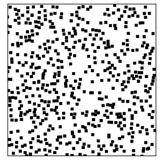
Figure 1: Representation of cells in the 2D CPM in the form of fluctuating rectangles. 539 cells (15% volume fraction) with $L_{x}^{(0)}=L_{y}^{(0)})=1.666667$ are shown.

Below we show very good agreement even for relatively large densities $\phi\simeq 0.3.$, between solutions of Eqs. (1), (I), (3) and ensemble average of stochastic trajectories of the microscopic CPM.

In Section II we introduce general microscopic equations describing motion of cells based on random fluctuations of their shapes and their interactions. We assume that each cell has a rectangular shape and consider stochastic differential equations for motion of cells as well as Smoluchowski equation (see e.g. Gardiner2004 ) for multi-cellular probability density function. In Section III we consider a particular case of microscopic cellular dynamics represented by the CPM without excluded volume interactions. Coefficients of Smoluchowski Eq. are derived from the CPM and stochastic dynamics of shapes and positions of cells are reduced to solutions of the closed equation describing positions of cells. In Section IV we consider cell motion and cell-cell interactions with collisions resolved through the jump processes resulting in equations (1), (I) and (3). In Section V numerics for the continuous macroscopic equations is compared with Monte Carlo simulations of the microscopic CPM. In Section VI we summarize main results and discuss future directions.

II Microscopic motion of cells

Motion of many eukaryotic cells and bacteria is accompanied by the random fluctuations of their shapes DD ; CM ; AM resulting in a random diffusion of center of mass of an isolated cell. Coefficient of such diffusion can be measured experimentally (see e.g. glazier2000 ). Fluctuations of cellular membrane in the presence of a chemical field are more likely in the direction of chemical gradient (for chemoattractant) of in opposite direction (for chemorepellent). Cells can also interact through direct contact which includes cell-cell adhesion and can be modeled using excluded volume principle. Cellular environment is highly viscous and inertia of cell can be ignored.

In this paper we assume that each cell has a fluctuating rectangular shape

Figure 2: 2D CPM cell representation. Grey and white colors are used to indicate cell body and surrounding extracellular matrix respectively. Cell can grow or shrink in $x$ and $y$ direction by adding or removing one row (or column) of pixels. pixels.

and allow random fluctuation of the dimensions of each rectangular cell (see Figures 1 and 2). Positions and shapes of cells are completely characterized by a finite set of dynamical variables in the configuration space: $X=({\bf R}_{1},{\bf L}_{1},{\bf R}_{2},{\bf L}_{2},\ldots,{\bf R}_{N},{\bf L}_{N})$, where $N$ is the total number of cells, ${\bf R}_{j}$ is a position of center of mass of $j$th cell, ${\bf L}_{j}$ is the size of $j$th cell in $D$ spatial dimensions. We consider $D=1$ and $D=2$ in which case cells are moving over substrate but results can be extended to the $D=3$ case. Microscopic description is provided by the multi-cellular probability density function (PDF) $P(X,t)$ defined as ensemble average $\langle\cdot\rangle$ over stochastic trajectories $({\bf R}_{j}^{\prime}(t),{\bf L}_{j}^{\prime}(t)),\ j=1,\ldots,N$ in the configuration space $X$: $P(X,t)=\langle\prod^{N}_{j=1}\delta({\bf R}_{j}-{\bf R}_{j}^{\prime}(t))\delta({\bf L}_{j}-{\bf L}_{j}^{\prime}(t))\rangle$ determined by solution of coupled stochastic equation

$$\frac{dX}{dt}={\bf A}(X,c,t)+\hat{B}(X,c,t)\xi(t),$$ (4)

and chemotaxis equation for the chemical field $c({\bf r},t)$. Here ${\bf r}$ is the spatial coordinate, ${\bf A}(X,t)$ is $2DN$-component vector, $\hat{B}(X,t)$ is $2DN\times 2DN$ matrix and $\xi(t)$ is $2DN$-component stationary Gaussian stochastic process with zero correlation time and zero mean

$$\langle\xi_{j}\rangle=0,\ \langle\xi_{i}(t)\xi_{j}(t^{\prime})\rangle=\delta_{i,j}\delta(t-t^{\prime}),\ i,j=1,\ldots,2DN,$$ (5)

where $\delta_{i,j}$ is a Kronecker’s symbol.

Application of the Stratonovich stochastic calculus to the Eq. (4) results in a ”multi-cellular” Fokker-Planck equation Gardiner2004 in configuration space $X$

$$\partial_{t}P(X,t)=-\nabla\cdot\big{[}{\bf v}P\big{]}+\nabla\cdot\big{[}\hat{D}\cdot\nabla P\big{]},$$

$${\bf v}={\bf A}-\frac{1}{2}\hat{B}\cdot\nabla\cdot\hat{B}^{T},$$

$$\hat{D}=\frac{1}{2}\hat{B}\cdot\hat{B}^{T},$$ (6)

where $\hat{D}(X,t)$ is a $2DN\times 2DN$ diffusion matrix, $\nabla=(\partial_{{\bf R}_{1}},\partial_{{\bf L}_{1}},\ldots,\partial_{{\bf R}_{N}},\partial_{{\bf L}_{N}})$ is the gradient operator in $2DN$ dimensions and $\hat{B}^{T}$ represents transposed matrix $\hat{B}$.

Dynamics of the chemical field $c({\bf r},t)$ is described by a diffusion equation

$$\partial_{t}c({\bf r},t)=\nabla_{\bf r}D_{c}\cdot\nabla_{\bf r}c+\int A(X,{\bf r},t)P(X,t)dX-\gamma c,$$ (7)

where $\nabla_{\bf r}$ is the gradient operator for the spatial coordinate and diffusion coefficient for the chemical field $D_{c}$ in general case can depend on ${\bf r}$ and $t$. Term $\int A(X,{\bf r},t)P(X,t)dX$ describes production of chemical by cells at the rate of $A(X,{\bf r},t)$ and $\gamma$ is a decay rate of the chemical. Cells produce chemical into intercellular space through their membranes. Therefore, in 3D case $A(X,{\bf r},t)$ is nonzero only at the cellular membrane. However, in 1D and 2D cells are moving on substrate, while chemical diffuse over entire three dimensional space so in 1D and 2D cases $A(X,{\bf r},t)$ is nonzero inside cells.

We assume that ${\bf v}$ has a form of a potential ${\bf v}=-\beta\nabla\Phi(X,t)$, where $\beta=1/T$ is the inverse effective temperature $T$ of the chemical fluctuations. Multi-cellular Fokker-Planck equation (II) is then reduced to multi-cellular Smoluchowski equation:

$$\partial_{t}P(X,t)=\nabla\cdot\hat{D}\cdot\Big{[}\nabla P+\beta(\nabla\Phi)P\Big{]},$$ (8)

(More general case of ${\bf v}$ being any function can be studied using similar approach.) If we neglect fluctuations of the cellular size ${\bf L}_{j}$ and chemotaxis, $c=0$, then Eq. (8) is similar to the Smoluchowski Eq. for the Brownian dynamics of colloidal particles (see e.g. JonesPusey1991 for a review) and Eq. (4) has a form of the Langevin equation for interacting Brownian particles with term $\hat{B}\xi$ representing thermal forces from solution in colloids. However, in general case considered here both chemotaxis and fluctuations of cellular shape are taken into account. Mechanisms of random fluctuation of cellular shape and cellular motion are still not completely clear and subject of active research DD ; CM ; AM .

We impose excluded volume constraint by choosing $\Phi(X,c)=\infty$ if any two cells overlap. We assume in what follows that all direct interactions between cells is of this type. We also allow indirect interactions between cells mediated by chemotaxis for which we choose

$$\left\{\begin{array}[]{cc}\Phi(X,c)&=-\sum\limits_{j=1}^{N}\chi({\bf L}_{j})c({\bf r},t)\Big{|}_{{\bf r}=X_{j}}+\Phi(X,c)\Big{|}_{c=0}\\ &\mbox{if cells do not overlap},\\ \Phi(X,c)&=\infty\\ &\mbox{if any pair of cells overlaps},\end{array}\right.$$ (11)

where $\chi({\bf L}_{j})$ represents strength of chemotactic interaction as a function of cellular sizes ${\bf L}_{j}$ and $\Phi(X,c)\Big{|}_{c=0}$ represents chemotaxis-independent terms of the potential. We assume for simplicity that chemotactic interaction depends only on gradient of $c({\bf r},t)$ at the center of mass of each cell. $\Phi(X,c)\Big{|}_{c=0}$ is also responsible for preserving cellular shape close to some equilibrium shape. Without this term shape (size) of each cell would experience unbounded random fluctuation which is non biological. We consider specific form of $\Phi(X,c)$ in Section III.3.

Our main goal is to derive a macroscopic equation describing dynamics of (total) cell probability density function

$$p({\bf r},t)=\sum\limits^{N}_{j=1}p_{j}({\bf r},t),$$ (12)

coupled with $c({\bf r},t)$, from microscopic equations (7) and (8). Here $p_{j}({\bf r},t)=\int P(X,t)\prod\limits^{N}_{l=1,\,l\neq j}d{\bf R}_{l}\prod\limits^{N}_{m=1}d{\bf L}_{m}\Big{|}_{{\bf R}_{j}={\bf r}}$ is a single-cell probability density function of the position of center of mass. After approximating $A(X,{\bf r},t)=a\sum^{N}_{j=1}\delta({\bf r}-{\bf R}_{j})$, $a=const$ and assuming that $D_{c}=const$, Eq. (7) is reduced with the help of Eq. (12) to Eq. (3). This approximation is justified because typical diffusion of a chemical is much faster than cell diffusion $D_{2}/D_{c}\ll 1.$ E.g. $D_{2}/D_{c}\sim 1/40-1/400$ for the cellular slime mold Dictyostelium HoferSherrattMaini1995 , $D_{2}/D_{c}\sim 1/30$ and for microglia cells and neutrophils LucaChavez-RossEdelstein-KeshetMogilner2003 ; GrimaPRL2005 .

III Microscopic cellular dynamics in Cellular Potts Model

Stochastic discrete models are used in a variety of problems dealing with biological complexity. One motivation for this approach is the enormous range of length scales of typical biological phenomena. Treating cells as simplified interacting agents, one can simulate the interactions of tens of thousands to millions of cells and still have within reach the smaller-scale structures of tissues and organs that would be ignored in continuum (e.g., partial differential equation) approaches. At the same time, discrete stochastic models including the Cellular Potts Model (CPM) can be made sophisticated enough to reproduce almost all commonly observed types of cell behavior Fram1 ; Cickovski05 ; Cickovski07 ; Knewitz06 ; Sozinova2006 ; JRSI . Recent book Anderson07 reviews many of the cell-based models.

The cell-based stochastic discrete CPM, which is an extension of the Potts model from statistical physics, has become a common technique for simulating complex biological problems including embryonic vertebrate limb development Cickovski05 ; Newman07 , tumor growth Jiang05 and vasculogenesis Merks . The CPM can be made sophisticated enough to reproduce almost all commonly observed types of cell behavior. It consists of a list of biological cells with each cell represented by several pixels, a list of generalized cells, a set of chemical diffusants and a description of their biological and physical behaviors and interactions embodied in the effective energy $E$, with additional terms to describe absorption and secretion of diffusants and extracellular materials. Distribution of multidimensional indices associated with lattice cites determines current cell system configuration. The effective energy of the system, $E$, mixes true energies, like cell-cell adhesion, and terms that mimic energies, e.g., volume constraint and the response of a cell to a gradient of an external field (including chemotactic filed) and area constraint.

III.1 Cellular Potts Model for cells of rectangular shape

For simplicity, we use in this paper CPM with rectangular cellular shapes. We also assume that all cells have the same type. The results can be extended to the general case of the CPM with arbitrary cellular shapes. Also, the approach is not limited to using CPM. For example, one could use microscopic off-lattice models NewmanMathBioEng2005 ; PLoS , where each cell is represented by a collection of subcellular elements with postulated interactions between them.

Notice that reduced representation of cells as fluctuating rectangles corresponds to intermediate level of description where fluctuations of cellular shapes are replaced by fluctuations of cellular sizes. Stochastic Eq. (4) or Smoluchowski Eq. (8) coupled with (3) can be used for modeling cell agregation.

In the CPM change of a cell shape evolves according to the classical Metropolis algorithm based on Boltzmann statistics and the following effective energy

$$E=E_{ECM}+E_{Adhesion}+E_{Perimeter}+E_{Field}.$$ (13)

If an attempt to change index of a pixel in a cell leads to energy change $\Delta E$, it is accepted with the probability

$$\Phi(\Delta E)=\left\{\begin{array}[]{cc}1,&\Delta E\leq 0\\ e^{-\beta\Delta E},&\Delta E>0,\end{array}\right.$$ (14)

where $1/\beta=T$ represents an effective boundary fluctuation amplitude of model cells in units of energy. Since the cells’ environment is highly viscous, cells move to minimize their total energy consistent with imposed constraints and boundary conditions. If a change of a randomly chosen pixels’ index causes cell-cell overlap it is abandoned. Otherwise, the acceptance probability is calculated using the corresponding energy change. The accepted pixel change attempt results in changing location of the center of mass and dimensions of the cell.

We consider 2D case with rectangular shape of each cell with sizes ${\bf L}_{j}=(L_{x,j},L_{y,j})$ and position of center of cellular mass at ${\bf R}_{j}=(x_{j},y_{j})$. Cell motion and changing shape are implemented by adding or removing a row or column of pixels (see Figure 2). We assume that cells can come into direct contact and that they interact over long distances through chemotaxis. Term $E_{ECM}$ in the Hamiltonian (13) phenomenologically describes net adhesion or repulsion between the cell surface and surrounding extracellular matrix: $E_{ECM}=\sum^{N}_{j=1}2J_{ECM}(L_{x,j}+L_{y,j})$, where $J_{ECM}$ is the binding energy per unit length of an interface. Term $E_{Adhesion}=J_{a}L_{contact}$ in the Hamiltonian (13) corresponds to the cell-cell adhesion, where $J_{a}$ is the binding energy per unit length of an interface and $L_{contact}$ is the total contact area between cells. Term $E_{\mathit{Perimeter}}$ defines an energy penalty function for dimensions of a cell deviating from the target values $L_{T_{x(y)}}$: $E_{Perimeter}=\sum^{N}_{j=1}\lambda_{x}(L_{x,j}-L_{T_{x}})^{2}+\lambda_{y}(L_{y,j}-L_{T_{y}})^{2}$ where $\lambda_{x}$ and $\lambda_{y}$ are Lagrange multipliers. Cells can move up or down gradients of both diffusible chemical signals (chemotaxis) and insoluble ECM molecules (haptotaxis) described by $E_{Field}=\sum^{N}_{j=1}\mu\,c({\bf R}_{j},t)L_{x,j}L_{y,j},$ where $\mu$ is an effective chemical potential.

In this paper we neglect cell-cell adhesion $J_{a}=0$ and the Hamiltonian (13) is reduced in 2D to the following expression

$$E(X,t)=\sum\limits^{N}_{j=1}E({\bf r},{\bf L},t)\Big{|}_{{\bf r}={\bf R}_{j},\ {\bf L}={\bf L}_{j}},$$

$$E({\bf r},{\bf L},t)=2J_{cm}(L_{x}+L_{y})+\lambda_{x}(L_{x}-L_{T_{x}})^{2}$$

$$\quad+\lambda_{y}(L_{y}-L_{T_{y}})^{2}+\mu\,c({\bf r})L_{x}L_{y}.$$ (15)

III.2 Master equation for discrete cellular dynamics

We now represent CPM dynamics by using $P({\bf r},{\bf L},t)$, probability density for any cell with its center of mass at ${\bf r}$ to have dimensions ${\bf L}$ at time $t.$ Which means that we consider one-cell PDF $P({\bf r},{\bf L},t)$ rather than $N$-cell PDF $P(X,t)$. Let $\epsilon\triangle r\times\epsilon\triangle r$ be the size of a lattice site with $\epsilon\ll 1$ and let vectors ${\bf e}_{1,2}$ indicate changes in $x$ and $y$ dimensions: ${\bf e}_{1}={\triangle r}(1,0),\ {\bf e}_{2}=\triangle r(0,1)$. We normalize the total probability to the number of cells: $\int P({\bf r},{\bf L},t)d{\bf r}d{\bf L}=N.$ $P({\bf r},{\bf L},t)$ used below should not be confused with multi-cellular probability density $P(X,t)$. Those depend on different arguments. Excluded volume constraint implies that position ${\bf r}^{\prime}$ and size ${\bf L}^{\prime}$ of any neighboring cell should satisfy $2|x-x^{\prime}|\geq L_{x}+L_{x}^{\prime}$, $2|y-y^{\prime}|\geq L_{y}+L_{y}^{\prime}$.

Discrete stochastic cellular dynamics under these conditions is described by the following master equation AlberChenLushnikovNewmanPRL2007 :

$$\begin{array}[]{cl }P({\bf r},{\bf L},t+\triangle t)=\sum_{j=1}^{2}\{\big{[}\frac{1}{2}-\Omega_{j,l}({\bf r}-\frac{\epsilon}{2}{\bf e}_{j},{\bf L}+\epsilon{\bf e}_{j};{\bf r},{\bf L},t)\end{array}$$

$$\begin{array}[]{cr cr}-\Omega_{j,r}({\bf r}+\frac{\epsilon}{2}{\bf e}_{j},{\bf L}+\epsilon{\bf e}_{j};{\bf r},{\bf L},t)-\Omega_{j,l}({\bf r}+\frac{\epsilon}{2}{\bf e}_{j},{\bf L}&\\ -\epsilon{\bf e}_{j};{\bf r},{\bf L},t)-\Omega_{j,r}({\bf r}-\frac{\epsilon}{2}{\bf e}_{j},{\bf L}-\epsilon{\bf e}_{j};{\bf r},{\bf L},t)\big{]}P({\bf r},{\bf L},t)&\\ +\Omega_{j,l}({\bf r},{\bf L};{\bf r}+\frac{\epsilon}{2}{\bf e}_{j},{\bf L}-\epsilon{\bf e}_{j},t)P({\bf r}+\frac{\epsilon}{2}{\bf e}_{j},{\bf L}-\epsilon{\bf e}_{j},t)&\\ +\Omega_{j,r}({\bf r},{\bf L};{\bf r}-\frac{\epsilon}{2}{\bf e}_{j},{\bf L}-\epsilon{\bf e}_{j},t)P({\bf r}-\frac{\epsilon}{2}{\bf e}_{j},{\bf L}-\epsilon{\bf e}_{j},t)&\\ +\Omega_{j,l}({\bf r},{\bf L};{\bf r}-\frac{\epsilon}{2}{\bf e}_{j},{\bf L}+\epsilon{\bf e}_{j},t)P({\bf r}-\frac{\epsilon}{2}{\bf e}_{j},{\bf L}+\epsilon{\bf e}_{j},t)&\\ +\Omega_{j,r}({\bf r},{\bf L};{\bf r}+\frac{\epsilon}{2}{\bf e}_{j},{\bf L}+\epsilon{\bf e}_{j},t)P({\bf r}+\frac{\epsilon}{2}{\bf e}_{j},{\bf L}+\epsilon{\bf e}_{j},t)\}.&\end{array}$$ (23)

We incorporate dynamics into MC algorithm by defining the time step $\triangle t$. Individual biological cells experience diffusion through random fluctuations of their shapes. Diffusive coefficient can be measured experimentally (see e.g. glazier2000 ). We choose $\triangle t$ to match experimental diffusion coefficient. Eq.(23) would determine a version of kinetic/dynamic MC algorithm (see e.g. kineticMC ) if $\triangle t$ were to be allowed to fluctuate. For simplicity we assume that $\triangle t=const$. Also $\Omega_{j,l}({\bf r},{\bf L};{\bf r}^{\prime},{\bf L}^{\prime},t)$ and $\Omega_{j,r}({\bf r},{\bf L};{\bf r}^{\prime},{\bf L}^{\prime},t)$ denote probabilities of transitions from a cell of length $L^{\prime}$ and center of mass at ${\bf r}^{\prime}$ to a cell of dimensions $L$ and center of mass at $\bf r$. Subscripts $l$ and $r$ correspond to transitions by addition/removal of a row/colomn of pixels from the rear/lower and front/upper ends of a cell respectively.

We define $\Omega_{j,l(r)}({\bf r},{\bf L};{\bf r}^{\prime},{\bf L}^{\prime})\equiv T_{l(r)}({\bf r},{\bf L};{\bf r}^{\prime},{\bf L}^{\prime})[1-\phi_{j,l(r)}({\bf r},\,{\bf L},t)]$ where $T_{l}(r)({\bf r},{\bf L};{\bf r}^{\prime},{\bf L}^{\prime},t)$ denote probabilities of transitions from a cell of length ${\bf L}^{\prime}$ and center of mass at ${\bf r}^{\prime}$ to a cell of dimensions $\bf L$ and center of mass at $\bf r$ without taking into account excluded volume principle and cell-cell adhesion. According to the CPM we have that $T_{l}({\bf r},{\bf L};{\bf r}^{\prime},{\bf L}^{\prime})=T_{r}({\bf r},{\bf L};{\bf r}^{\prime},{\bf L}^{\prime})=\frac{1}{8}\Phi\Big{(}E({\bf r},{\bf L})-E({\bf r}^{\prime},{\bf L}^{\prime})\Big{)}$ where the factor of $1/8$ is due to the fact that there are potentially 8 possibilities for increasing or decreasing of $L_{x}$ and $L_{y}$ (it means that we can add/romove pixel from any 4 sides of rectangular cell). Second term $\phi_{j,l(r)}({\bf r},\,{\bf L},t)$ takes into account contact interactions between cells. It includes contributions from 3 possible types of stochastic jump processes due to contact interactions between cells: (a) a cell adheres to another one, (b) two adhered cells dissociate from each other due to membrane fluctuations, (c) membranes of two adhered cells are prevented from moving inside each other (due to excluded volume constraint) resulting in a negative sign of a contribution to a jump probability. If neither of these 3 processes happens at given time step then $\phi_{j,l(r)}({\bf r},\,{\bf L},t)=0$.

III.3 Macroscopic limit of master equation and mean-field approximation

Eq. (23) is however not closed because one has to know multi-cellular probability density to determine $\phi_{j,l(r)}({\bf r},\,{\bf L},t)$. One could use BBGKY-type hierarchy McQuarrie2000 similar to the one used in kinetic theory of gases, which expresses iteratively $n$-cell PDF through $n+1$-cell PDF with truncation at some order. This is however extremely difficult and ineffective for large $n$. Instead, we develop in Section IV a nonperturbative approach to derivation of Eqs. (1) and (I).

In previous work alber1 ; alber2 ; AlberChenLushnikovNewmanPRL2007 we studied a macroscopic limit $\epsilon\ll 1$ of master Eq. (23) by both neglecting contact interactions between cells alber1 ; alber2 and including contact interactions in mean-field approximation AlberChenLushnikovNewmanPRL2007 , which represents simplest closure for BBGKY-type hierarchy. If contact interactions are neglected, then $\phi_{j,l(r)}({\bf r},\,{\bf L},t)=0$ and (23) yields in macroscopic limit $\epsilon\ll 1$ alber1 ; alber2 :

$$\partial_{t}P({\bf r},{\bf L},t)=D_{2}(\nabla^{2}_{\bf r}+4\nabla^{2}_{\bf L})P+8D_{2}\beta\lambda_{x}\partial_{L_{x}}(\tilde{L}_{x}P)$$

$$+8D_{2}\beta\lambda_{y}\partial_{L_{y}}(\tilde{L}_{y}P)+D_{2}\beta L_{x}L_{y}\mu\partial_{\bf r}\big{[}P\nabla_{\bf r}c\big{]},$$

$$\tilde{L}_{x}=\frac{1}{\lambda_{x}}\big{[}J_{cm}+\lambda_{x}(L_{x}-L_{T_{x}})+\frac{1}{2}L_{y}\mu c({\bf r})\big{]},$$

$$\tilde{L}_{y}=\frac{1}{\lambda_{y}}\big{[}J_{cm}+\lambda_{y}(L_{y}-L_{T_{y}})+\frac{1}{2}L_{x}\mu c({\bf r})\big{]},$$

$$D_{2}=\frac{(\triangle r)^{2}}{16\triangle t},\nabla^{2}_{\bf r}=\partial_{x}^{2}+\partial_{y}^{2},\quad\nabla^{2}_{\bf L}=\partial_{L_{x}}^{2}+\partial_{L_{y}}^{2}.$$ (24)

Similar Eq. in 1D case (with only coordinate $x$ and length $L_{x}$ present) was obtained in Ref. alber1 .

Mean field approximation assumes decoupling of multi-cellular PDF,

$$P(X,t)=N^{-N}\prod\limits^{N}_{j=1}P({\bf r},{\bf L}_{j},t)\Big{|}_{{\bf r}={\bf R}_{j}},$$ (25)

where factor $N^{-N}$ is due to an assumed normalization $\int P({\bf r},{\bf L},t)d{\bf r}d{\bf L}=N.$ Mean field approximation is exact if contact interactions are neglected. This holds since we assumed above that chemotaxis depended on averaged density (12) only. Eq. (25) results in decoupling of Eq. (8) into independent Eqs. for $P({\bf R}_{j},{\bf L}_{j},t)$ for all $j$. This allows direct comparison of Eq. (III.3) with Eq. (8) and yields that diffusion matrix has a diagonal form with main diagonal $D_{2}(1,1,4,4,1,1,4,4\ldots)$ in 2D. For 1D and 3D cases numbers $1$ and $4$ repeat themselves with period $1$ and $3$, respectively.

Further comparison of (8), (11) and (III.3) leads to expression $\chi({\bf L}_{j})=\ L_{x,j}L_{y,j}\mu$ and

$$\Phi(X,t)=E(X,t),$$ (26)

where $E(X,t)$ is given by (III.1).

Taking into account contact cell-cell interaction (excluded volume) yields that Eq. (25) is not exact any more. Also, potential $\Phi(X,t)$ is given by (26) only if cells do not overlap. Otherwise $\Phi(X,t)=\infty$ according to (11).

III.4 Boltzmann-like distribution and macroscopic equation for cellular density

From Eqs. (III.1), (14) and (III.3) it follows that typical fluctuations of cell sizes $\tilde{L}_{x(y)}$ are determined by $\beta\lambda_{x(y)}\tilde{L}_{x(y)}^{2}\sim 1$. Suppose $x_{0}$ and $y_{0}$ are typical scales of $P({\bf r},{\bf L},t)$ with respect to $x$ and $y$. We assume that $\beta x_{0}^{2}\lambda_{x}\gg 1$ and $\quad\beta y_{0}^{2}\lambda_{y}\gg 1$, meaning that $x_{0}\gg\tilde{L}_{x},\ y_{0}\gg\tilde{L}_{y}$. We also assume that chemical field $c({\bf r},t)$ is a slowly varying function of ${\bf r}$ on the scale of typical cell length meaning that $x_{c}/L_{x}\gg 1,\quad y_{c}/L_{y}\gg 1,$ where $x_{c}$ and $y_{c}$ are typical scales for variation of $c({\bf r},t)$ in $x$ and $y$. We also make an additional biologically relevant assumption that $4\lambda_{x}\lambda_{y}\gg\mu^{2}c({\bf r},t)^{2}$ meaning that change of typical cell size due to chemotaxis $\delta L^{(chemo)}_{x(y)}$ is small $|\delta L^{(chemo)}_{x(y)}|\ll L^{(min)}_{x(y)}.$

If all these conditions are satisfied then we found by using both solutions of Eq. (III.3) and MC simulations of CPM with general initial conditions, that PDF $P({\bf r},{\bf L},t)$ quickly converges in $t$ at each spatial point ${\bf r}$ to the following Boltzmann - like form

$$P({\bf r},{\bf L},t)=P_{Boltz}({\bf r},{\bf L})p({\bf r},t),$$ (27)

where

$$P_{Boltz}({\bf r},{\bf L})=\frac{1}{Z({\bf r})}\exp(-\beta\triangle E_{length})$$ (28)

is a Boltzmann - like distribution depending on ${\bf r}$ and $t$ only through $c({\bf r},t)$,

$$\triangle E_{length}=E({\bf r},{\bf L})-E_{min}$$

$$=\lambda_{x}L_{x}^{\prime 2}+\lambda_{y}L_{y}^{\prime 2}+L^{\prime}_{x}L^{\prime}_{y}\mu c({\bf r}),{\bf L}^{\prime}={\bf L}-{\bf L}^{(min)}.$$ (29)

Here $E_{min}=E({\bf r},{\bf L}^{(min)})$ is the minimal value of (III.1) achieved at ${\bf L}={\bf L}^{(min)}$:

$$E_{min}=E({\bf r},{\bf L}^{(min)}),$$

$$L_{x}^{(min)}=\frac{-4\lambda_{y}(J_{cm}-\lambda_{x}L_{T_{x}})+2(J_{cm}-\lambda_{y}L_{T_{y}})\mu c({\bf r})}{4\lambda_{x}\lambda_{y}-\mu^{2}c({\bf r})^{2}},$$

$$L_{y}^{(min)}=\frac{-4\lambda_{x}(J_{cm}-\lambda_{y}L_{T_{y}})+2(J_{cm}-\lambda_{x}L_{T_{x}})\mu c({\bf r})}{4\lambda_{x}\lambda_{y}-\mu^{2}c({\bf r})^{2}}$$

(30)

and $Z({\bf r},t)=(2\epsilon\triangle r)^{2}\sum_{{\bf L}}\exp(-\beta\triangle E_{length})\simeq\frac{2\pi}{\beta\sqrt{4\lambda_{x}\lambda_{y}-\mu^{2}c({\bf r},t)^{2}}}$ is an asymptotic formula for a partition function as $\epsilon\to 0$. (See alber1 for details about convergence rate for the case without contact interactions)

Also, under these conditions we can use Eq. (27) to integrate Eq. (III.3) over $\bf L$ which results in the following evolution equation for the the cellular probability density $p({\bf r},t)=\int(P({\bf r},{\bf L},t)d{\bf L}$ alber1 ; alber2 :

$$\partial_{t}p=D_{2}\nabla^{2}_{\bf r}p-\chi_{0}\nabla_{\bf r}\cdot\big{[}p\,\nabla_{\bf r}c({\bf r},t)\big{]},$$ (31)

where $\chi_{0}=-D_{2}\mu\beta L_{x}^{(0)}L_{y}^{(0)}$ and

$$L_{x}^{(0)}=L_{T_{x}}-J_{cm}/\lambda_{x},$$

$$L_{y}^{(0)}=L_{T_{y}}-J_{cm}/\lambda_{y}$$ (32)

correspond to $L_{x(y)}^{(min)}$ from (III.4) provided we neglect chemotaxis.

Eq. (31) together with $(\ref{ceqmacroscopic1})$ form a closed set which coincides with the classical Keller-Segel system KS . It has a finite time singularity (collapse) and was extensively used for modeling aggregation of bacterial colonies HerreroVelazquez1996 ; BrennerConstantinKadanoff1999 . We show below that near singularity contact interactions between cells could prevent collapse.

Eqs. similar to $(\ref{pottscontinuous3})$ and $(\ref{ceqmacroscopic1})$ for the case of contact interactions (excluded volume constraint) has been obtained in mean-field approximation AlberChenLushnikovNewmanPRL2007 . These Eqs. significantly slow down collapse in comparison with $(\ref{pottscontinuous3})$ and $(\ref{ceqmacroscopic1})$. They still have collapsing solutions if initial density is not small. (These Eqs. are applicable only for small densities.)

IV Beyond mean-field approximation and regularization of collapse

Main purpose of this paper is to derive macroscopic Eqs. which do not have collapse (blow up of solutions in finite time) for arbitrary initial densities and are in good agreement with microscopic stochastic simulations for large cellular densities. This requires one to go beyond mean-field approximation.

We conclude from the previous section that random changes of cellular lengths result in random walks of centers of mass of cells during the time between cell ”collisions”. Significant simplification in comparison with Eq. (II) is that we have now explicit dependence on spatial coordinate $\bf r$ but not on $\bf L$. We use below notation $(L_{x}^{(0)},L_{y}^{(0)})$ for average size of a cell neglecting change of that size due to chemotaxis. For CPM $(L_{x}^{(0)},L_{y}^{(0)})$ are given by (III.4). If we neglect chemotaxis (i.e. set $c=0$) then during time between collision cell probability density $p({\bf r},t)$ is described by linear diffusion Eq. which follows from Eq. (31):

$$\partial_{t}p=D_{2}\nabla^{2}_{\bf r}p.$$ (33)

In a similar way, two-cell probability density $p({\bf r}_{1},{\bf r}_{2},t)$ is described by linear diffusion for two independent variables ${\bf r}_{1},{\bf r}_{2}$:

$$\partial_{t}p=D_{2}(\nabla^{2}_{{\bf r}_{1}}+\nabla^{2}_{{\bf r}_{2}})p.$$ (34)

$p({\bf r}_{1},{\bf r}_{2},t)$ represents probability density of a cells $1$ and $2$ having centers of mass at ${\bf r}_{1}$ and ${\bf r}_{2}$ at time $t$, respectively. After making change of variables

$${\bf r}={\bf r}_{1}-{\bf r}_{2},\quad{\bf R}=({\bf r}_{1}+{\bf r}_{2})/2,$$ (35)

where variable ${\bf r}$ describes relative motion of cells and variable ${\bf R}$ describes motion of ”center of mass” of two cells, Eq. (34) takes the following form

$$\partial_{t}p=2D_{2}\nabla^{2}_{{\bf r}}p+\frac{D_{2}}{2}\nabla^{2}_{{\bf R}}p.$$ (36)

Each collision involving cell $1$ or $2$ modifies both $p({\bf r},t)$ and $p({\bf r}_{1},{\bf r}_{2},t)$. In other words, it effects random walk of each colliding cell.

We describe first the effect of collisions due to excluded volume constraint between cells in 1D case. Consider a pair of neighboring cells which in 1D always remain neighbors. We assume that at the time of collision two colliding cells have the same size. Generally this is not true because sizes of cells continuously fluctuate with lengthscale $\delta L_{x}\sim 1/(\beta^{1/2}\lambda_{x}^{1/2}).$ However, we assume as before that these fluctuation are small $|\delta L_{x}|\ll L_{x}^{(0)}$ which justifies our approximation. Collision is defined as two cells being in direct contact at given moment of time and one of them trying to penetrate into another. Collison is prevented by excluded volume constraint. In the continuous limit $\epsilon\to 0$ each collision takes infinitesimally small time. After collision cells move away from each other so they are not in direct contact any more. Instead of explicitly describing each of these collisions we use an assumption that two cells are identical and view each collision as exchange of positions of two cells Rost1984 ; BodnarVelazquez2005 . From such point of view cells do not collide at all but simply pass through each other. They both experience random walk as point objects (cells) without collisions according to Eqs. (33) and (36) in the domain free from other cells (free domain). (The volume of such free domain per cell, which has dimension of length in 1D, is on average $(1-L_{x}^{(0)}p(x,t))/p(x,t)$.) This means that we are considering collective diffusion JonesPusey1991 of cellular density instead of trajectories of individual cells. In contrast, self-diffusion describes mean-square displacement of an individual cell as a function of time JonesPusey1991 . This approach might be important for describing propagation of one cell type through space occupied by cells of another type. In this paper we consider only collective diffusion.

While trajectories of cells in free domain are continuous, positions of cells in physical space change instantaneously at each collision by $L_{x}$ for the cell colliding from the left and by $-L_{x}$ for the cell colliding from the right. The effective rate of cell diffusion is enhanced as free space becomes smaller with growth of cellular volume fraction. Let’s assume that at the initial time $t=t_{0}$ centers of mass of two cells are separated by an average distance $1/p(x,t)$ and that these two cells collide for the first time (meaning that previous collisions of each cell involved collision with cells other than these two). This yields that their centers of mass are separated by distance $L_{x}^{(0)}$ at $t=t_{0}.$ If moving reference frame is set at one of the cells then other will experience random walk with doubled diffusion coefficient $2D_{2}$ (as seen from Eq. (36)), where $D_{2}$ is a diffusion coefficient of each cell in the stationary reference frame. Relative motion of two cells in moving reference frame corresponds to random walk of a point-wise cell with diffusion coefficient $2D_{2}$. Consider continuous random walk. Number of returns to the initial position $x=L_{x}^{(0)}$ during any finite time interval after $t_{0}$ is infinite meaning that number of collisions between given pair of cells in physical space is infinite. However, successive collisions effectively cancel each other since they change positions of cells by $\pm L_{x}^{(0)}.$ What really matters is whether total number of collision is even or odd. For even number of collisions total contribution of collisions is zero. While for odd number of collisions contribution to the flux of probability for the left cell (at time $t_{0}$) $\propto L_{x}^{(0)}$ and for the right cell $\propto-L_{x}^{(0)}.$ Because total number of collisions is infinite, the probabilities to have even or odd number of collisions are equal to $1/2.$ While the average distance between center of mass of cells is $1/p(x,t)$, the average distance between boundaries of two neighboring cells in physical domain is

$$\triangle x=1/p(x,t)-L_{x}^{(0)}.$$ (37)

When separation between surfaces of two cells after collision reaches $\triangle x$ from (37) we determine that ”extended collision” between the pair of cells is over. Namely, two cells are not closer to each other than to other neighboring cells any more. Therefore, probability of them colliding with each other is not higher any more than probability of them colliding with other cells. This extended collision includes infinitely many ”elementary” collisions but its final contribution depends only on whether the total number of such collision is even or odd.

To find average time of extended collision we solve diffusion Eq. in moving frame

$$\partial_{t}p_{m}=2D_{2}\nabla^{2}_{x}p_{m}$$ (38)

with reflecting boundary condition $\partial_{x}p_{m}(L_{x}^{(0)},t)=0$ at $x=L_{x}^{(0)}$ and absorbing boundary condition $p_{m}(L_{x}^{(0)}+\triangle x,t)=0$ at $x=L_{x}^{(0)}+\triangle x$. Reflecting boundary condition means that cell does not cross point $x=L_{x}^{(0)}$. Instead of crossing $x=L_{x}^{(0)}$ cells exchange positions at each collision. Absorbing boundary condition corresponds to the ”escape point” of cell from extended collision. Initial condition is $p_{m}(x,t_{0})=\delta(x-L_{x}^{(0)})$ which is defined by initial zero distance between surfaces of two cells. Solution of the Eq. (38) with these initial and boundary conditions results in calculation of the mean first-passage time (escape time) $T_{esc}$, which is equal to the extended collision time in our case. To find $T_{esc}$ we use a backward Fokker-Planck Eq.

$$\partial_{t_{1}}p(x_{2},t_{2}|x_{1},t_{1})=U^{\prime}(x_{1})\partial_{x_{1}}p(x_{2},t_{2}|x_{1},t_{1})$$

$$-D_{0}\nabla^{2}_{x_{1}}p(x_{2},t_{2}|x_{1},t_{1})$$ (39)

(see e.g. Gardiner2004 ), where $p(x_{2},t_{2}|x_{1},t_{1})$ is the conditional probability density for transition from $(x_{1},t_{1})$ to $(x_{2},t_{2})$. $D_{0}$ is the diffusion coefficient and $U(x)$ is an arbitrary potential. In 1D case $U(x)=0$ and $D_{0}=2D_{2}$.

For convenience of the reader we provide here a derivation of $T_{esc}$ which is similar to the one from Ref. Gardiner2004 . Probability that cell remains inside an interval $(0,\triangle x)$ at time $t$, provided it was located at $x$ at $t=t_{0}$, is given by $G(x,t)\equiv\int^{\triangle x}_{0}p(x^{\prime},t|x,t_{0})dx^{\prime}$. Using the stationarity of the random walk $p(x^{\prime},t|x,t_{0})=p(x^{\prime},0|x,t_{0}-t)$ we obtain from (IV) that

$$\partial_{t}G=-U^{\prime}(x)\partial_{x}G+D_{0}\nabla^{2}_{x}G.$$ (40)

Mean escape time $T_{esc}(x)$ for a cell located at $x$ at $t=t_{0}$ is

$$T_{esc}(x)=-\int\limits^{\infty}_{t_{0}}(t-t_{0})\partial_{t}G(x,t)dt=\int\limits^{\infty}_{t_{0}}G(x,t)dt.$$ (41)

Integrating Eq. (40) over $t$ from $t_{0}$ to $\infty$ and using initial normalization $G(x,t_{0})=1$ results in

$$-U^{\prime}(x)\partial_{x}T_{esc}(x)+D_{0}\nabla^{2}_{x}T_{esc}(x)=-1.$$ (42)

Reflecting and absorbing boundary conditions for $p$ result in similar boundary conditions for $T_{esc}(x):$

$$\partial_{x}T_{esc}(x)\Big{|}_{x=L_{x}^{(0)}}=0,\quad T_{esc}(x)\Big{|}_{x=L_{x}^{(0)}+\triangle x}=0,$$ (43)

which allows us to solve boundary value problem (42),(43) explicitly:

$$T_{esc}(x)=D_{0}^{-1}\int\limits^{L_{x}^{(0)}+\triangle x}_{x}\exp{\big{[}D_{0}^{-1}U(x^{\prime})\big{]}}dx^{\prime}$$

$$\times\int\limits^{x^{\prime}}_{L_{x}^{(0)}}\exp{\big{[}-D_{0}^{-1}U(x^{\prime\prime})\big{]}}dx^{\prime\prime}.$$ (44)

Initial condition implies that $T_{esc,1}=T_{esc}(L_{x}^{(0)})$ and yields extended collision time in 1D:

$$T_{esc,1}=\frac{(\triangle x)^{2}}{4D_{2}}.$$ (45)

Consider mean square displacement of position of each cell during extended collision in the stationary frame. We use notations $(\triangle x)^{2}_{1}$ and $(\triangle x)^{2}_{2}$ for mean square displacement of cells $1$ and $2$, respectively, in the stationary frame. Using (35) we obtain that $(\triangle x)^{2}_{1}+(\triangle x)^{2}_{2}=\frac{(\triangle x)^{2}}{2}+2(\triangle X)^{2}$, where $X={\bf R}$ in 1D. Because of the symmetry between cells $1$ and $2$ the following relation holds $(\triangle x)^{2}_{1}=(\triangle x)^{2}_{2}=\frac{(\triangle x)^{2}}{4}+(\triangle X)^{2}$. Center of mass of two cells experiences random walk with diffusion coefficient $D_{2}/2$ (see Eq. (36)) and $(\triangle X)^{2}=T_{esc,1}D_{2}=\frac{(\triangle x)^{2}}{4},$ $(\triangle x)^{2}_{1}=(\triangle x)^{2}_{2}=\frac{(\triangle x)^{2}}{2}$.

Now recall that with probability $1/2$ cells exchange positions during extended collision meaning that in expression for $(\triangle x)^{2}_{1,2}$ with probability $1/2$ term $(\triangle x)^{2}$ should be replaced by $(2L_{x}^{(0)}+\triangle x)^{2}$ resulting in the total mean square displacement for cell $1$ or $2$

$$(\triangle x)^{2}_{total}=\frac{1}{2}\Big{(}\frac{(\triangle x)^{2}}{2}+\frac{(2L_{x}^{(0)}+\triangle x)^{2}}{2}\Big{)}.$$ (46)

From Eqs. (37),(45) and (46) we obtain effective (nonlinear) diffusion coefficient for the cell probability density

$$D_{1,effective}=\frac{(\triangle x)^{2}_{total}}{2T_{esc,1}}=D_{2}\Big{[}\frac{1+(L_{x}^{(0)})^{2}p^{2}}{(1-L_{x}^{(0)}p)^{2}}\Big{]}.$$ (47)

In simulations described below we often use not very large number of cells $N$. In case of finite $N$ each given cell can collide with $N-1$ remaining cells which gives extra factor $(N-1)/N$ and allows one to rewrite the effective diffusion coefficient (47) as follows

$$D_{1,effective}=D_{2}\Big{[}\frac{1+(1-N^{-1})(L_{x}^{(0)})^{2}p^{2}}{(1-(1-N^{-1})L_{x}^{(0)}p)^{2}}\Big{]}.$$ (48)

The effective diffusion (48) results in 1D nonlinear diffusion Eq.:

$$\partial_{t}p=D_{2}\nabla_{\bf r}\cdot\Big{[}\frac{1+(1-N^{-1})(L_{x}^{(0)})^{2}p^{2}}{(1-(1-N^{-1})L_{x}^{(0)}p)^{2}}\nabla_{\bf r}p\Big{]}$$

$$-\chi_{0}\nabla_{\bf r}\cdot\big{[}p\,\nabla_{\bf r}c({\bf r},t)\big{]}.$$ (49)

Here we added chemotaxis term from Eq. (31) which is well justified provided $x_{c}\gg\triangle x$ (see also previous section).

Now consider 2D case. First consider cells with disk-shaped form instead of cells of rectangular shapes (i.e. cellular shapes fluctuating around a disk) with average diameter $L_{x}^{(0)}$. Assume, similar to 1D case, that $t_{0}$ is the time of the first collision between two given cells. Previous collisions of each of these cells involved cells other then these two. We also average over angles relative to the center of one of these two cells which implies that cells collide at time $t=t_{0}$ with equal probability at every angle. In that approximation there is rotational symmetry in the moving frame and all variables depend only on the radial variable $r\equiv|{\bf r}|$ but do not depend on angular variables. Change of variables in Fokker-Planck Eq. $\partial_{t}p=2D_{2}\nabla^{2}_{\bf r}p$ results in

$$\partial_{t}{\tilde{p}}=-2D_{2}\partial_{r}\frac{\tilde{p}}{r}+2D_{2}\nabla^{2}_{r}\tilde{p},$$ (50)

where $\tilde{p}\equiv rp.$ Eq. (50) is equivalent to the 1D Fokker-Planck Eq. with potential $U(r)=-2D_{2}\log(r)$. Backward Fokker-Planck Eq. (IV) with $x=r$, and the same $U(r)$ yields in a way similar to Eqs. (40)-(45), an extended collision time (mean escape time)

$$T_{esc,2}=\frac{\triangle x(2L_{x}^{(0)}+\triangle x)}{8D_{2}}-\frac{\big{[}L_{x}^{(0)}\big{]}^{2}}{4D_{2}}\log{\left(1+\frac{\triangle x}{L_{x}^{(0)}}\right)}.$$ (51)

We assume again that during extended collision time cells on average span entire space, i.e.

$$\frac{\pi}{4}(L_{x}^{(0)}+\triangle x)^{2}=p^{-1}.$$ (52)

Using Eqs. (46), (51) and (52) we obtain effective diffusion coefficient in 2D (here and below the average disk diameter is $L\equiv L_{x}^{(0)}$):

$$D_{2,effective}=\frac{(\triangle x)^{2}_{total}}{4T_{esc,2}}$$

$$=D_{2}\Big{[}\frac{1+\pi L^{2}p}{1-\pi L^{2}p+\pi L^{2}p\log(\pi L^{2}p)}\Big{]},$$ (53)

which after modification to include effect of a finite $N$ similar to the one used in 1D case, results in

$$D_{2,effective}=D_{2}\Big{[}\frac{1+(1-N^{-1})\pi L^{2}p}{1-(1-N^{-1})\pi L^{2}p+(1-N^{-1})\pi L^{2}p\log(\pi L^{2}p)}\Big{]},$$ (54)

Eq. (54) yields the following nonlinear diffusion Eq. for cells fluctuating around disk-shaped form

$$\partial_{t}p=D_{2}\nabla_{\bf r}\cdot\Big{[}\frac{1+(1-N^{-1})\pi L^{2}p}{1-(1-N^{-1})\pi L^{2}p+(1-N^{-1})\pi L^{2}p\log(\pi L^{2}p)}\nabla_{\bf r}p\Big{]}-\chi_{0}\nabla_{\bf r}\cdot\big{[}p\,\nabla_{\bf r}c({\bf r},t)\big{]}.$$ (55)

Notice that both 1D effective diffusion coefficient (48) and 2D effective diffusion coefficient (54) depend only on the volume fraction $\phi$ ($\phi=L_{x}^{(0)}p$ in 1D and $\phi=\pi L^{2}p$ in 2D). Based on that we propose that the effective diffusion coefficient for 2D rectangles also depends only on the volume fraction $\phi=L_{x}^{(0)}L_{y}^{(0)}p$, which results in the nonlinear diffusion Eq. for cells of rectangular shape

$$\partial_{t}p=D_{2}\nabla_{\bf r}\cdot\Big{[}\frac{1+(1-N^{-1})L_{x}^{(0)}L_{y}^{(0)}p}{1-(1-N^{-1})L_{x}^{(0)}L_{y}^{(0)}p+(1-N^{-1})L_{x}^{(0)}L_{y}^{(0)}p\log(L_{x}^{(0)}L_{y}^{(0)}p)}\nabla_{\bf r}p\Big{]}-\chi_{0}\nabla_{\bf r}\cdot\big{[}p\,\nabla_{\bf r}c({\bf r},t)\big{]}.$$ (56)

Numerical simulations in the next section confirm that Eq. (56) agrees very well with the MC simulations of microscopic dynamics.

In macroscopic limit $N\gg 1$ factor $(1-N^{-1})$ is replaced by $1$ in Eqs. (IV), (55) and (56), which yields Eqs. (1) and (I).

If volume fraction $\phi\to 1$ then nonlinear diffusion in Eqs. (1) and (I) diverges. Thus we do not expect any blow up of the solution contrary to Eq. (31). Global existence of Eqs. (1) and (I) together with Eq. (3) can be studied in a way similar to HillenWang2007 .

V Numerical results and application to vasculogenesis

V.0.1 One dimensional cell motion

Figure 3 demonstrates simulation of 1D motion of cells represented in the form of fluctuating rods. Numerical solution of the continuous model was obtained using a pseudo-spectral scheme. For both the CPM simulation and numerics of the continuous model we used periodic boundary conditions, simulation time was $t_{end}=200$ and values of other parameters were chosen as follows: $\triangle r=1$, $L_{T_{x}}=L_{T_{x}}=3$, $\lambda_{x}=\lambda_{y}=1.5$, $\epsilon=0.01$ $J_{cm}=2$, $\beta=15$, $N=8$, $\mu=0$. Simulation was performed on the spatial domain $0\leq x<100$ and the initial cell density distribution was $p({\bf r},0)=k_{0}e^{-((x-50)/10)^{4}}$ with $k_{0}$ determined by normalization $N=8$. Figure 3 shows simulations of the CPM (curve a), numerical solutions of the macroscopic model without excluded volume interactions (31) (curve b), macroscopic Eq. (V.0.1) (curve c), and macroscopic Eq. (IV) (curve d).

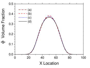
Figure 3: Volume fraction $\phi=L_{x}^{(0)}p(x,t_{end})$ for the 1D cellular motion as a function of $x$. Curve (a): Monte Carlo simulations of the CPM. Curve (b): solution of the Eq. (31). Curve (c): solution of the Eq. (V.0.1). Curve (d) solution of the Eq. (IV).

Here Eq.

$$\partial_{t}p=D_{2}\nabla_{\bf r}\cdot\Big{[}\frac{1}{(1-(1-N^{-1})L_{x}^{(0)}p)^{2}}\nabla_{\bf r}p\Big{]}$$

$$-\chi_{0}\nabla_{\bf r}\cdot\big{[}p\,\nabla_{\bf r}c({\bf r},t)\big{]},$$ (57)

was derived from the equation of state for the 1D hard rod fluid PercusJStatPhys1976 which allows one to determine collective diffusion coefficient from static structure factor and compressibility (see e.g. JonesPusey1991 ; Gomer1990 ).

Figure 3 demonstrates that solution of the Eq. (IV) is in much better agreement with CPM than both Eqs. (31) and (V.0.1). While the difference between the CPM simulation and solutions of the Eq. (31) and Eq. (V.0.1) is small but clearly exceeds the error in MC simulations. Difference between MC simulation and solution of the Eq. (IV) is within an accuracy of the MC simulations.

Difference between CPM and Eq. (V.0.1) is due to the fact that the equation of state for the 1D hard rod fluid was calculated in Ref. PercusJStatPhys1976 from grand canonical partition function LandauLifshitzV5 while diffusion of cells is a nonequilibrium phenomenon resulting in the corrections to the equilibrium partition function. Numerous attempts have been made to describe dynamics of interacting Brownian particles (see KawasakiJStatMech2008 and reference there in). Note also that difference between CPM and Eq. (31) results is not so dramatic in 1D as in 2D because in 1D Keller-Segel model does not support collapse BrennerConstantinKadanoff1999 .

V.0.2 Two dimensional cell motion with chemotaxis

Figures 4 and 5 demonstrate a very good agreement between typical CPM simulation and numerical solution of the continuous model Eq. (56). Both simulations were performed on a square domain $0\leq x,y\leq 100$ over simulation time $t_{end}=400$. Simulation parameters’ values are as follows $\triangle r=1$, $L_{T_{x}}=L_{T_{y}}=4.4$, $\lambda_{x}=\lambda_{y}=1.5$, $J_{cm}=2$, $\beta=15$, $\mu=0.1$, $\epsilon=0.01$ and $N=15$. Chemical field concentration is chosen in the form of $c(x,y)=0.2[1-e^{-\frac{(x-65)^{2}+(y-60)^{2}}{144}}]$ and does not depend on time. Initial cell density is chosen in the form of $p_{0}(x,y)=k_{0}e^{-[\frac{(x-50)^{2}+(y-50)^{2}}{100}]^{5}}$, where $k_{0}$ is a constant that normalizes the integral of the cell density to $N=15$. Numerical solution of the continuous model has been obtained using pseudo-spectral scheme with $200\times 200$ Fourier modes. A large number of CPM simulations (600000) have been run on a parallel computer cluster to guarantee a representative statistical ensemble.

Numerics for Eq. (31) significantly differs from CPM simulations indicating that excluded volume interactions are important in the chosen range of values of parameters.

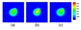
Figure 4: $p(x,y,t)$ in 2D as a function of $(x,y)$ for (a) Monte Carlo simulation of CPM, (b) Eq. (31) and (c) Eq. (56).

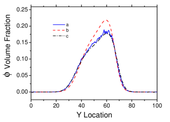
Figure 5: Cross sections of the volume fraction $\phi=L_{x}^{(0)}L_{y}^{(0)}p(x_{0},y,t)$ in 2D for (a) CPM simulation, (b) Eq. (31) and (c) Eq. (56). All cross sections are at the same position: $x_{0}=57.75$.

V.0.3 Application to Vasculogenesis

To test the model we studied effect of the chemical production rate on the network formation. Our previous results AlberChenLushnikovNewmanPRL2007 were limited to relatively small chemical production rate $a\leq 0.2$ in Eq. (3) because otherwise chemotaxis resulted in cellular density which was too high for applying mean-field approximation. Here we use macroscopic Eqs. (56), (3) and compare numerical results with the CPM simulations. Figure 6 shows series of simulations with different chemical production rates $a=0.5,\ a=1.5$ and $a=3.0$. Simulations start with initially dilute populations of cells moving on a substrate in a chemotactic field, subject to an excluded volume constraint. Both CPM and continuous model simulation results indicate that stripe patterns are obtained for high chemical production rates. Higher chemical production rate, by strengthening the chemotaxis and cell aggregation process, eventually leads to higher pattern density with smaller average distance between two neighboring stripes. Structures of the resulting networks obtained using discrete and continuous models are very similar to each other as well as to the one obtained experimentally for a population of endothelial cells cultured on a Matrigel film Serini .

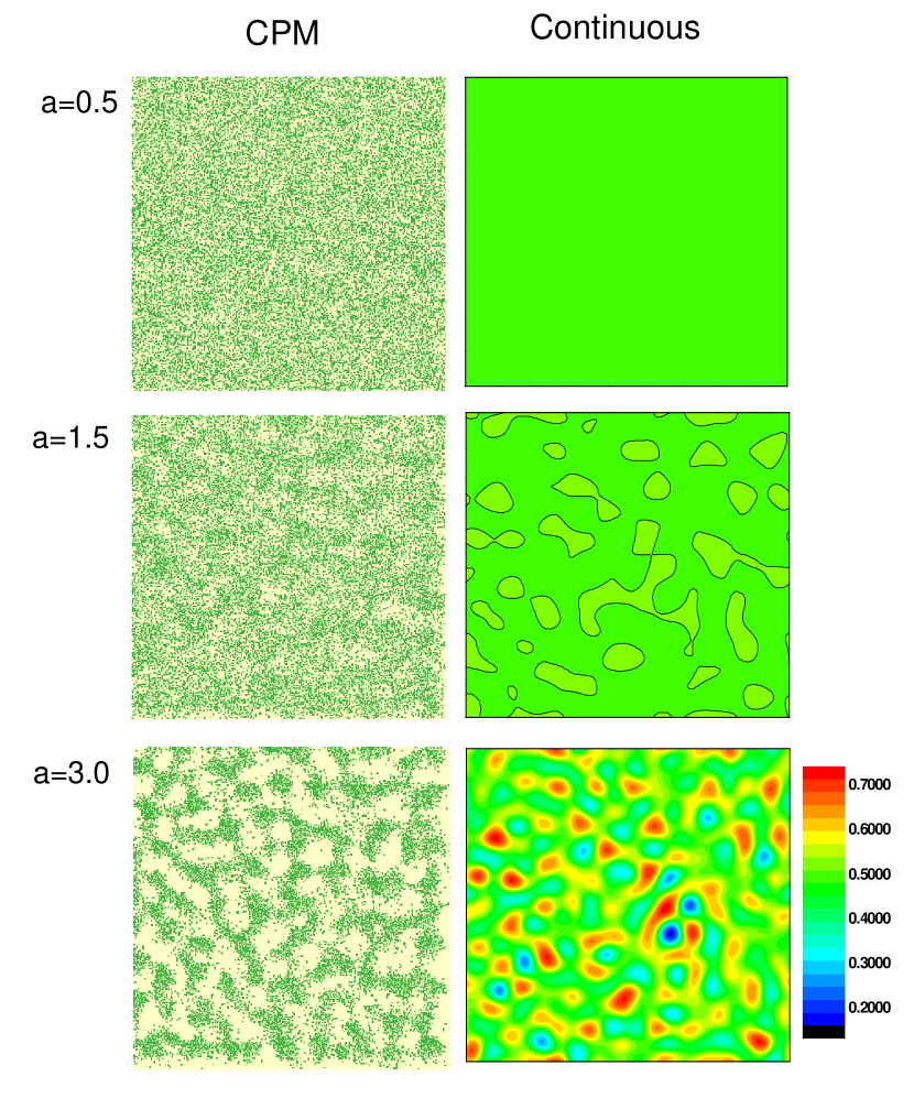
Figure 6: Simulation of early vascular network formation with different chemical production rates $\alpha$. $\triangle r=1$, $L_{T_{x}}=L_{T_{y}}=0.6$, $\lambda_{x}=\lambda_{y}=1.5$, $J_{cm}=0.002$, $\beta=15$, $\mu=-0.1$, $D_{c}=0.5$, $\gamma=0.014$, $\Delta t_{c}=\epsilon^{2}\Delta t=0.01,\epsilon=0.1$, $t_{end}=60$. In the Monte Carlo CPM simulation $N=15000$ cells were randomly distributed in a domain $0\leq x,y\leq 100$ with initial chemical field at zero. In the continuous model, a uniform initial cell density distribution with $5\%$ random fluctuation was used. Scale bar is in units of the volume fraction $\phi$.

VI Summary and discussion

We have derived macroscopic continuous Eqs. (1) and (I) coupled with Eq. (3) for describing evolution of cellular density in the chemical field, from microscopic cellular dynamics. Microscopic cellular model includes many individual cells moving on a substrate by means of random fluctuations of their shapes, chemotactic and contact cell-cell interactions. Contrary to classical Keller-Segel model, solutions of the obtained Eqs. (1), (I) (3) do not collapse in finite time and can be used even when relative volume occupied by cells $\phi$ is quite large. This makes them much more biologically relevant then earlier introduced systems. We compared simulations of macroscopic Eqs. with Monte Carlo simulations of microscopic cellular dynamics for the CPM and demonstrated a very good agreement for $\phi\simeq 0.3$. For larger density we expect transition to glass state JonesPusey1991 . It was demonstrated that combination of the CPM and derived continuous model can be applied to studying network formation in early vasculogenesis. We are currently working on an important problem in vasculogenesis of simulating self-diffusion JonesPusey1991 of one type of cells through dense population of other types of cells.

This work was partially supported by NSF grants DMS 0719895 and IBN-0344647.

References

- (1) A. Gamba, D. Ambrosi, A. Coniglio, A. de Candia, S. DiTalia, E. Giraudo, G. Serini, L. Preziosi and F. Bussolino,, Phys. Rev. Lett. 90, 118101 (2003).
- (2) G. Serini, D. Ambrosi, E. Giraudo, A. Gamba, L. Preziosi, F. Bussolino. The EMBO Journal 22 1771 (2003).
- (3) P. Carmeliet, Nature Medicine 6, 389 (2000).
- (4) R. M. H. Merks, S. Brodsky, M. Goligorksy, S. Newman, J. Glazier, Dev. Biol. 289, 44 (2006).
- (5) P. A. Rupp, A. Czirok, and C. D. Little, Development 131, 2887 (2004).
- (6) A. Szabo, E. D. Perryn, A. Czirok, Phys. Rev. Lett. 98, 038102 (2007).
- (7) S. Christley, M. Alber, and S. Newman. PLoS Computational Biology. 3(4), e76 (2007).
- (8) E. F. Keller and L. A. Segel, J. Theor. Biol. 30, 225 (1971).
- (9) W. Alt, J. Math. Biol. 9, 147 (1980).
- (10) H. G. Othmer and A. Stevens, SIAM J. Appl. Math. 57 No.4 1044 (1997).
- (11) A. Stevens, SIAM J. Appl. Math. 61, 172 (2000).
- (12) T. J. Newman and R. Grima, Phys. Rev. E, 70, 051916 (2004).
- (13) M. A. Herrero, and J. J. L Velázquez. Math. Ann. 306, 583 (1996).
- (14) M. P. Brenner, P. Constantin, L. P. Kadanoff, A. Shenkel, and S. C. Venkataramani, Nonlinearity 12, 1071 (1999).
- (15) S. Turner, J. A. Sherratt, K. J. Painter and N. J. Savill, Phys. Rev. E 69, 021910 (2004).
- (16) T. J. Newman, Biosciences and Engeneering 2, 611 (2005).
- (17) M. Alber, N. Chen, T. Glimm, and P.M. Lushnikov, Phys. Rev. E. 73, 051901 (2006).
- (18) M. Alber, N. Chen, T. Glimm, and P. M. Lushnikov. Single-Cell-Based Models in Biology and Medicine, Series: Mathematics and Biosciences in Interaction. Eds. A.R.A. Anderson, M.A.J. Chaplain, K.A. Rejniak. Birkhauser Verlag Basel/Switzerland (2007).
- (19) M. Alber, N. Chen, P. M. Lushnikov, and S. A. Newman. Phys. Rev. Lett. 99, 168102 (2007).
- (20) C.W. Gardiner, Handbook of stochastic methods for physics, chemistry, and the natural sciences, Springer-Verlag, (2004).
- (21) H.G. Döbereiner, B.J. Dubin-Thaler, J.M. Hofman, H.S. Xenias, T.N. Sims, G. Giannone, M.L. Dustin, C.H. Wiggins, and M.P. Sheetz, Phys Rev Lett. 97, 038102 (2006).
- (22) J. Coelho Neto, and O.N. Mesquita, Philos. Trans. A 366 319 (2008).
- (23) U. Agero, C.H. Monken, C. Ropert, R.T. Gazzinelli, and O.N. Mesquita, Phys. Rev. E. 67, 051904 (2003).
- (24) J.P. Rieu, J.-P. Rieu, A. Upadhyaya, J. A. Glazier, N. B. Ouchi, Y. Sawada,, Biophys. J. 79, 1903 (2000)
- (25) R. B. Jones and P.N. Pusey, Annu. Rev. Phys. Chem., 42, 137 (1991).
- (26) T. Hofer, J.A. Sherratt, and P. K. Maini, Physica D 85, 425 (1995).
- (27) M. Luca, A. Chavez-Ross, L. Edelstein-Keshet, and A. Mogilner, Bull. Math. Biol. 65, 693 (2003).
- (28) R. Grima, Phys. Rev. Lett. 95, 128103 (2005).
- (29) T. M. Cickovski, C. Huang, R. Chaturvedi, T. Glimm, H. Hentschel , M. S. Alber, J. A. Glazier, S. A. Newman, J. A. Izaguirre. IEEE/ACM Trans. Comput. Biol. Bioinformatics, 2(4), 273 (2005)
- (30) T. M. Cickovski, K. Aras, M. Swat, R. Merks, T. Glimm, H. Hentschel , M. S. Alber, J. A. Glazier, S. A. Newman, J. A. Izaguirre, Computing in Science and Engineering, 9, 50 (2007)
- (31) R. Chaturvedi, C. Huang, B. Kazmierczak, T. Schneider, J. A. Izaguirre, T. Glimm, H. G. Hentschel, J. A. Glazier, S. A. Newman, M. S. Alber, J. R. Soc. Interface 2 237 (2005)
- (32) M. A. Knewitz, J. C. M. Mombach, Comput Biol Med, 36(1), 59 (2006)
- (33) O. Sozinova, Y, Jiang, D, Kaiser and M, S. Alber, Proc. Natl. Acad. Sci. 103(46), 17255 (2006)
- (34) Z. Xu, N. Chen, M. M. Kamocka, E. D. Rosen and M. S. Alber, Journal of the Royal Society Interface. 5, 705 (2008).
- (35) A. Anderson, M. Chaplain and Rejniak K, Single Cell-Based Models in Biology and Medicine Eds. Birkha ser, (2007)
- (36) S. Newman, S. Christley, T. Glimm, H. Hentschel, B. Kazmierczak, Y. Zhang, J. Zhu and M. S. Alber. Curr. Top. Dev. Biol. 81, 311 (2008)
- (37) Y. Jiang, J. Pjesivac-Grbovic, C. Cantrell and J. P. Freyer, Biophys J, 89(6), 3884 (2005)
- (38) Y. Wu, Y. Jiang, D. Kaiser and M. Alber, PLoS Computational Biology. 3, 12, e253 (2007).
- (39) A. B. Bortz, M. H. Kalos and J. L. Lebowitz, J. Comp. Physics 17, 10 (1975).
- (40) D.A. McQuarrie, Statistical Mechanics, University Science Books (2000).
- (41) H. Rost, Lecture notes in Math., 1059, 127 (1984).
- (42) M. Bodnar, and J. J. L. Velázquez., Math. Meth. Appl. Sci. 28, 1757 (2005).
- (43) Z. Wang, and T. Hillen, Chaos 17, 037108 (2007).
- (44) J.K. Percus, J. Stat. Phys. 15, 505 (1976).
- (45) R. Gomer, Rep. Prog. Phys, 53, 917 (1990).
- (46) L. D. Landau and E. M. Lifshitz, Statistical Physics, 3rd Edition, Butterworth-Heinemann (1984).
- (47) B. Kim, and K. Kawasaki, J. Stat. Mech. - Theor. and Exp. P02004 (2008).