A Computation of the Expected Number of Posts in a Finite Random Graph Order

Abstract

A random graph order is a partial order achieved by independently sprinkling relations on a vertex set (each with probability $p$) and adding relations to satisfy the requirement of transitivity. A post is an element in a partially ordered set which is related to every other element. Alon et al. [2] proved a result for the average number of posts among the elements $\{1,2,\ldots,n\}$ in a random graph order on $\mathbb{Z}$. We refine this result by providing an expression for the average number of posts in a random graph order on $\{1,2,\ldots,n\}$, thereby quantifying the edge effects associated with the elements $\mathbb{Z}\backslash\{1,2,\ldots,n\}$. Specifically, we prove that the expected number of posts in a random graph order of size $n$ is asymptotically linear in $n$ with a positive $y$-intercept. The error associated with this approximation decreases monotonically and rapidly in $n$, permitting accurate computation of the expected number of posts for any $n$ and $p$. We also prove, as a lemma, a bound on the difference between the Euler function and its partial products that may be of interest in its own right.

1 Introduction

Several definitions of random partial orders can be found in the combinatorics literature. If the number $n$ of elements of the underlying set is fixed, perhaps the most natural definition is that of “uniform random order,” in which we pick a member of the set of $n$-element posets uniformly at random. Although no practical way is known of generating posets according to this definition for large $n$, it is known that as $n\to\infty$ most of them are “3-level” posets [6]. In this case, increasing $n$ leads to posets with a greater width but not a greater height, on average, because of the growth in the number of relations per element. A second definition is that of “random $k$-dimensional order”, for some integer $k$, in which one picks $k$ linear orders on $n$ elements uniformly at random (in other words, $k$ randomly chosen permutations of the set $\{1,2,...,n\}$), and then takes their intersection. The resulting posets are of dimension $k$ by construction, and some of their properties are known [13].

A third definition, and the one we will mainly be interested in here, is that of “random graph order” which depends on a parameter $p\in(0,1)$. To obtain a partial order of this type, one first generates a random graph on the vertex set $\{1,2,...,n\}$ by including an edge $(i,j)$ with probability $p$ for each pair of vertices $i$ and $j$; one then turns the graph into a directed one by converting each edge $(i,j)$ into a relation $i\prec j$ in the partial order if $i<j$ (in the usual order on the integers); and, finally, one imposes transitive closure by adding relations so that $i\prec k$ whenever there exists a $j$ such that $i\prec j$ and $j\prec k$. Several properties of random graph orders, such as width, height, and dimension have been studied [1]. In particular, it is known [1] that the expected height of a random graph order on $n$ elements grows linearly with $n$.

In the physics literature, random graph orders are also known as “transitive percolation” because they arise in a special case of the theory of directed percolation [7], where non-local bonds in a 1-dimensional lattice are turned on with probability $p$. They also play a prominent role among the stochastic sequential growth models that have been proposed for the classical version of the dynamics of causal sets [9], and this is the context that most directly motivates our work. A causal set [4] is a partially ordered set that is locally finite, meaning that the interval or Alexandrov set $I(i,j):=\{l\mid i\prec l\prec j\}$ is finite for every pair with $i\prec j$. In the causal set approach to quantum gravity (for a recent review, see Ref. [5]), the poset is seen as a discrete spacetime. The partial order corresponds to the causal relations among its elements, and “$i\prec j$” can be read as “$i$ causally precedes $j$”, while volumes of spacetime regions correspond to the cardinality of the appropriate subsets of the poset. The final theory is expected to assign a spacetime volume of the order of $\ell_{\rm P}^{4}$ to each element, where $\ell_{\rm P}:=\sqrt{G\hbar/c^{3}}=1.6\times 10^{-33}$ cm is the Planck length.

A post in a poset is an element that is related to every other element in the poset. In other words, each post $n$ divides the ordered set into the subset of elements that precede it, its “past”, and the subset of elements that follow it, its “future”. In the causal set interpretation the spacetime “pinches off” at $n$; this can be seen as the zero-spatial-volume singularity at the end of a collapsing phase for the universe and the beginning of a new expanding phase. Thus, a first set of desirable conditions for transitive percolation to be considered as a physically reasonable way of generating discrete spacetimes is that if a random graph order develops multiple posts, the number of elements between two posts be allowed to grow sufficiently large for that region to be able to model our observed universe.

It has been known for some time [2] that infinite random graph orders have an infinite number of posts. However, the occurrence of posts in finite random graph orders has not been studied as extensively. We begin by revisiting random graph orders on $\mathbb{N}$ and then analyzing finite posets. Roughly speaking, we find in our analysis that “edge effects” are small but non-negligible. In the infinite case, the probability that element $n$ is a post approaches a constant value fairly rapidly. In a finite case, the expected number posts is well approximated by this limiting probability times the size of the set plus a small positive offset. We illustrate our conclusions with numerical simulations.

2 Infinite Random Graph Orders

We begin by calculating the probability that any given element in an infinite random graph order is a post. In order to express this probability succinctly we define $q=1-p$,

$$\lambda_{k}(q)=(1-q)(1-q^{2})\cdots(1-q^{k}),\quad{\rm and}\quad\kappa(q)=\lambda_{\infty}(q)=\lim_{k\rightarrow\infty}\lambda_{k}(q).$$

The function $\kappa(q)$ is known as the Euler function, and it has been studied in considerable detail [12]. In particular, $\kappa(q)>0$ for all $0<q<1$. We now prove a theorem for one-way infinite random graph orders similar to the result of Alon, et al. [2] that the probability that an element in a random graph order on $\mathbb{Z}$ is a post is $\kappa^{2}(q)$.

Theorem 2.1.

In a random graph order on $\mathbb{N}$ with probability $0<p<1$, the probability that any given element $k$ is a post is given by

$$\begin{array}[]{rcl}\Pr(k\mbox{ is a post})&=&\lambda_{k-1}(q)\,\lambda_{\infty}(q)\\ &\gtrsim&\kappa^{2}(q),\end{array}$$ (1)

where by $\gtrsim$, we mean “greater than and, for large $k$, approximately equal to.”

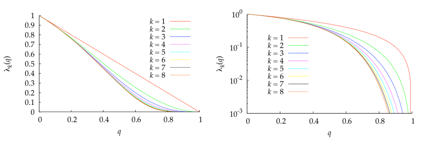
Figure 1: Plot of $\lambda_{k}(q)$ as a function of $q$ for $k=1,...,8$ (from top to bottom).

Plots of $\lambda_{k}(q)$ as functions of $q$ for various values of $k$ (see Fig. 1) illustrate the rate of the convergence of $\lambda_{k}(q)$ to $\kappa(q)$. Because of this convergence, the similarity in (1) holds for “most” $k\in\mathbb{N}$. This observation suggests two intuitively plausible results. The first is that with unit probability, there are infinitely many posts in any random graph order. This result was first proved by Alon et al. [2]. Although the original result was for random graph orders on $\mathbb{Z}$, the proof is easily adapted to partial orders on $\mathbb{N}$. The second result is that the mean spacing between posts is $\kappa^{-2}(q)$. Equivalently, the expected number of posts after $N$ stages is well-approximated by $\kappa^{2}N$. This information on the structure of random graph orders is of the type we are interested in from the point of view of their possible applications as models of discrete spacetimes, and in the next section we will consider it in more detail.

Proof 2.2 (Proof of theorem.).

If $k$ is related to $k-1$, $k-2$, $\ldots$, $k-i+1$ (for $1<i<k$), then the probability that $k-i\nprec k$ is $q^{i}$, since by transitivity the only way for this to happen is for $k-i$ to be unrelated to each of $k-i+1$, $k-i+2$, …, $k$. Hence we find that

$$\Pr(k-i\prec k\mid k-1\prec k\;\wedge\;k-2\prec k\;\wedge\ldots\wedge\;k-i+1\prec k)=1-q^{i},$$

where we have used the notation $\Pr(A|B)$ for the conditional probability of $A$ given $B$ and $\wedge$ for logical and. Repeatedly decomposing the probability that $k$ is related to each element before it yields the expression

$$\Pr(k\text{ related to all previous }m) =\Pr(k-1\prec k)\cdot\Pr(k-2\prec k\mid k-1\prec k)\cdot\ldots$$

$$\hskip 45.52458pt\cdot\Pr(1\prec k\mid 2\prec k\;\wedge\ldots\wedge\;k-1\prec k)$$

$$=(1-q)(1-q^{2})\cdots(1-q^{k-1})$$

$$=\lambda_{k-1}(q)$$

$$>\kappa(q).$$ (2)

The inequality follows because the partial products of $\lambda_{\infty}(q)$ are strictly decreasing.

On the other hand, the same logic that led to (2) shows the probability that $n$ is related to every later element is given by

$$\begin{array}[]{rcl}\Pr(n\text{ related to every later }m)&=&\Pr(n\prec n+1)\cdot\Pr(n\prec n+2\mid n\prec n+1)\cdot\ldots\\ &=&\prod_{j=1}^{\infty}(1-q^{j})\\ &=&\kappa(q).\end{array}$$

Moreover, the events $m\prec n$ for $m<n$ and $n\prec m$ for $m>n$ are independent. If transitive closure were to relate $m<n$ and $k>n$ in a manner involving $n$, then $n$ would be the middle element and both relations $m\prec n$ and $n\prec k$ would exist a priori. Hence the event “$n$ is a post” will occur if and only if the two preceding, independent events occur, which has probability

$$\Pr(n\mbox{ is a post}) =\Pr(n\mbox{ related to all }m<n)\cdot\Pr(n\mbox{ related to all }m>n)$$

$$=\lambda_{n-1}(q)\,\lambda_{\infty}(q)$$

$$\gtrsim\kappa^{2}(q),$$

as desired.

3 Posts in Finite Random Graph Orders

From the results for infinite graph orders we expect that, to a good approximation, the expected number of posts in an $n$-element poset is $N_{\rm posts}(n)=\kappa^{2}(q)\,n$. In fact, the mean number of posts among the elements $\{1,2,\ldots,n\}$ in a random graph order on $\mathbb{Z}$ is equal to $\kappa^{2}(q)\,n$ [3]. However, this number should be smaller than the expected number of posts in a random graph order on $\{1,2,\ldots,n\}$—and appreciably smaller for small $n$—because elements near the edge are significantly likely to be related to all the elements in $\{1,2,\ldots,n\}$ but not all the elements in $\mathbb{Z}$. We have carried out numerical simulations of transitive percolation with different values of $p$ and $n$; Fig. 2 shows the resulting values of $N_{\rm posts}$ plotted versus $n$ for a fixed $p$. From this plot, one may see that for large $n$ the number of posts is well approximated by a line with a small offset. We will now prove the following theorem.

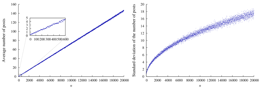
Figure 2: Average and standard deviation of the number of posts in a random graph order versus number of elements, for $p=0.35$. For each value of $n$, four hundred $n$-element causal sets were generated, and the average and standard deviation of the numbers of posts are shown. The sampled values of $n$ are the multiples of 5 up to 20,000. Notice in the inset graph that the average number of posts seems to be well fit by a line with positive $y$-intercept.

Theorem 3.1.

For all $0<q<1$, there exists a sequence of real numbers $\{b_{n}(q)\}_{n=1}^{\infty}$ so that for all $n\geq 1$, $b_{n}(q)$ is strictly between 0 and 1 and the expectation value $\langle N_{n,q}\rangle$ of the number of posts in a transitively percolated causal set on $\{1,\,2,\,3,\,\ldots,\,n\}$ with probability $p=1-q$ satisfies

$$\langle N_{n,q}\rangle=\kappa^{2}(q)\cdot n+b_{n}(q)\,.$$ (3)

Moreover, $\{b_{n}(q)\}_{n=2}^{\infty}$ is strictly monotonically decreasing to a positive limit $b(q)$ given by the expression

$$b(q)=2\kappa(q)\sum_{k=0}^{\infty}(\lambda_{k}(q)-\kappa(q)).$$ (4)

For notational convenience, we will drop the explicit dependence of $\kappa^{2}$ and $b_{n}$ on $q$. We also introduce the abbreviations

$$\mu_{n}:=\prod_{i=n}^{\infty}(1-q^{i}),\qquad S_{n}:=\sum_{k=1}^{\infty}\frac{q^{nk}}{\lambda_{k}}.$$

Notice that $\mu_{1}=\kappa$. In order to prove the theorem, we first establish the following estimates.

Lemma 3.2.

For all $n\geq 2$, we have

$$(\lambda_{n-1}-q^{n})S_{n}<q^{n},$$ (5)

and

$$\lambda_{n-1}-\kappa<q^{n}.$$ (6)

Proof 3.3.

If $\lambda_{n-1}-q^{n}$ is not positive, then (5) clearly holds since $S_{n}$ and the right-hand side are positive. So suppose that $\lambda_{n-1}-q^{n}$ is positive. Because the $\lambda_{k}$ are monotonically decreasing in $k$ and $n-1\geq 1$, we may replace $\lambda_{n-1}$ with $\lambda_{1}$ to find

$$(\lambda_{n-1}-q^{n})S_{n} ~{}\leq~{}(\lambda_{1}-q^{n})\left(\sum_{k=1}^{\infty}\frac{q^{nk}}{\lambda_{k}}\right).$$

Distributing and using the definitions of $\lambda_{k}$ gives

$$(\lambda_{1}-q^{n})\left(\sum_{k=1}^{\infty}\frac{q^{nk}}{\lambda_{k}}\right) =\sum_{k=1}^{\infty}\frac{q^{nk}}{\prod_{i=2}^{k}(1-q^{i})}-\sum_{k=1}^{\infty}\frac{q^{n(k+1)}}{\prod_{i=1}^{k}(1-q^{i})}$$

$$=\sum_{k=1}^{\infty}\frac{q^{nk}}{\prod_{i=2}^{k}(1-q^{i})}-\sum_{k=2}^{\infty}\frac{q^{nk}}{\prod_{i=1}^{k-1}(1-q^{i})},$$

where we have reindexed the second sum in the second line. Separating the first term in the first sum, we get

$$=q^{n}+\sum_{k=2}^{\infty}\frac{q^{nk}}{\prod_{i=2}^{k}(1-q^{i})}-\sum_{k=2}^{\infty}\frac{q^{nk}}{\prod_{i=1}^{k-1}(1-q^{i})}$$

$$=q^{n}+\sum_{k=2}^{\infty}\frac{q^{nk}}{\prod_{i=2}^{k-1}(1-q^{i})}\left[\frac{1}{1-q^{k}}-\frac{1}{1-q}\right]$$

$$<q^{n}.$$

because all the terms in the summation are negative. This establishes (5).

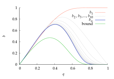
Figure 3: The offset terms $b_{n}(q)=\langle N_{n,1-q}\rangle-\kappa^{2}(q)n$, for $n=1$ (dashed red), $n=2,3,\ldots,10$ (dashed gray), and $n\to\infty$ (solid blue). The bound for $b(q)$ obtained by taking $n\to\infty$ in (10) is shown in green.

Now we will show that (6) follows from (5). We use the following well-known identity [8], which holds for all complex $|x|<1$, $|z|<1$:

$$\prod_{m=1}^{\infty}(1-x^{m}z)=\left(\sum_{k=0}^{\infty}\frac{x^{k}z^{k}}{\prod_{i=1}^{k}(1-x^{i})}\right)^{-1}.$$ (7)

For completeness, we include a proof of (7). Define

$$f(x,z)=\frac{1}{\prod_{m=1}^{\infty}(1-x^{m}z)},$$ (8)

and consider $f$ as a function of $z$ for fixed $|x|<1$. Since $\prod_{m=1}^{\infty}(1-x^{m}z)\neq 0,$ we can write it as $\exp\left(\sum_{m=1}^{\infty}\log(1-x^{m}z)\right)$. This, in turn, may be written

$$\exp\left(-\sum_{m=1}^{\infty}\sum_{k=1}^{\infty}\frac{(x^{m}z)^{k}}{k}\right)=\exp\left(-\sum_{k=1}^{\infty}\sum_{m=1}^{\infty}\frac{x^{mk}z^{k}}{k}\right).$$

This shows that $f$ is analytic throughout the unit disk $|z|<1$. Therefore we can write $f$ as a power series in $z$: $f(x,z)=\sum_{k=0}^{\infty}c_{k}(x)z^{k}$. Now it is easy to see from (8) that $f(x,xz)=(1-xz)\,f(x,z)$, and this implies $x^{k}\,c_{k}(x)=c_{k}(x)-x\,c_{k-1}(x)$. Noticing that $c_{0}(x)=1$ and solving this recursive relationship gives (7).

Finally, set $x=q$ and $z=q^{n-1}$, and apply (7) to the definition of $\mu_{n}$ to obtain:

$$\mu_{n}=\left(\sum_{k=0}^{\infty}\frac{q^{nk}}{\lambda_{k}}\right)^{-1}.$$

Notice that $\mu_{n}=(1+S_{n})^{-1}$, and rearrange (5) to get $\lambda_{n-1}\,S_{n}<(1+S_{n})\,q^{n}$. Putting these together, we have

$$\lambda_{n-1}-\kappa=\lambda_{n-1}(1-\mu_{n})=\frac{\lambda_{n-1}\,S_{n}}{1+S_{n}}<q^{n},$$

as desired.

Lemma 2 provides a very useful bound regarding the convergence of the partial products of $\kappa$ to their limiting value. We will use the bound several times to prove statements that involve expressions of the form $\lambda_{n-1}-\kappa$ or $1-\mu_{n}$. While there are more efficient ways to compute the Euler function[12], Lemma 2 also shows that even the naive products converge reasonably well: the error is strictly bounded by $q^{n}$, a considerable improvement—especially for $q$ close to 1—over the obvious estimate that the partial products are of order $O(q^{n})$. Slater[11] first used (7) to compute the Euler function numerically but did not observe its implications for the naive products.

Proof 3.4 (Proof of theorem.).

First, we define the random variables

$$X_{k}=\left\{\begin{array}[]{ll}1&\text{$k$ is a post}\\ 0&\text{$k$ is not a post}\end{array}\right.\qquad(k=1,2,\ldots,n).$$

Then $N_{n,q}=\sum_{k=1}^{n}X_{k}$ and, by linearity, $\langle N_{n,q}\rangle=\sum_{k=1}^{n}\langle X_{k}\rangle=\sum_{k=1}^{n}\text{Pr($k$ is a post)}$. From the proof of Theorem 2.1, we know

$$\text{Pr($k$ is a post)}=\prod_{i=1}^{k-1}(1-q^{i})\prod_{j=1}^{n-k}(1-q^{j}).$$

Substituting in the definitions of $\mu_{k}$ and $\kappa$ gives:

$$\langle N_{n,q}\rangle =\sum_{k=1}^{n}\frac{\kappa}{\mu_{k}}\,\frac{\kappa}{\mu_{n-k+1}}=\kappa^{2}\sum_{k=1}^{n}\frac{1}{\mu_{k}\,\mu_{n-k+1}}.$$

Define the “offset” quantities $b_{n}$ according to (3):

$$b_{n}=\langle N_{n,q}\rangle-n\,\kappa^{2}=\kappa^{2}\sum_{k=1}^{n}\left[\frac{1}{\mu_{k}\,\mu_{n-k+1}}-1\right].$$ (9)

First, we produce a lower bound on $b_{n}$. As $x<-\!\log\left(1-x\right)$ for $x\in(0,1)$, we have

$$-\log\mu_{k}=-\sum_{i=k}^{\infty}\log(1-q^{i})>\sum_{i=k}^{\infty}q^{i}=\frac{q^{k}}{1-q},$$

which implies that

$$\mu_{k}<\exp\left(-\frac{q^{k}}{1-q}\right).$$

From this we obtain

$$\frac{1}{\mu_{k}\,\mu_{n-k+1}}-1~{}>~{}\exp\left(\frac{q^{k}+q^{n-k+1}}{1-q}\right)-1~{}>~{}\frac{q^{k}+q^{n-k+1}}{1-q}.$$

Substituting the previous equation into (9) gives

$$b_{n}~{}>~{}\kappa^{2}\sum_{k=1}^{n}\frac{q^{k}+q^{n-k+1}}{1-q}~{}=~{}\frac{2\,q\,\kappa^{2}(1-q^{n})}{(1-q)^{2}},$$ (10)

where we have used the fact that the exponents $n-k+1$ and $k$ range over the same set of values as $k=1,2,\ldots,n$. This establishes that the sequence $\{b_{n}\}_{n=2}^{\infty}$ is bounded below by a positive quantity (see Fig. 3).

Next, we prove that for every $n\geq 2$ we have $b_{n}>b_{n+1}$. We calculate the difference $b_{n}-b_{n+1}$:

$$\kappa^{-2}(b_{n}-b_{n+1}) =\sum_{k=1}^{n}\frac{1}{\mu_{k}\mu_{n-k+1}}-n-\sum_{k=1}^{n+1}\frac{1}{\mu_{k}\mu_{n-k+2}}+n+1$$

$$=1-\frac{1}{\mu_{1}\mu_{n+1}}+\sum_{k=1}^{n}\frac{1}{\mu_{k}}\left(\frac{1}{\mu_{n-k+1}}-\frac{1}{\mu_{n-k+2}}\right).$$

Recall that summation by parts (see, e.g., Ref [10]) says that for general sequences $\{x_{n}\}$ and $\{y_{n}\}$, if we define $X_{n}=\sum_{k=1}^{n}x_{k}$, we have $\sum_{k=1}^{n}x_{k}y_{k}=X_{n}y_{n}+\sum_{k=1}^{n-1}X_{k}(y_{k}-y_{k+1})$. Taking $x_{k}=1/{\mu_{n-k+1}}-1/{\mu_{n-k+2}}$ and $y_{k}=1/\mu_{k}$ in this formula, we get (notice that $X_{k}$ is a telescoping sum):

$$=1-\frac{1}{\mu_{1}\mu_{n+1}}+\frac{1}{\mu_{n}}\left(\frac{1}{\mu_{1}}-\frac{1}{\mu_{n+1}}\right)+\sum_{k=1}^{n-1}\left[\left(\frac{1}{\mu_{n-k+1}}-\frac{1}{\mu_{n+1}}\right)\left(\frac{1}{\mu_{k}}-\frac{1}{\mu_{k+1}}\right)\right].$$

The quantity $1/{\mu_{n-k+1}}-1/{\mu_{n+1}}$ in the first set of parentheses in the sum can be made smaller by replacing $\mu_{n-k+1}^{-1}$ with $\mu_{n}^{-1}$ as $\mu_{n}$ is monotonically increasing in $n$. Performing the remaining telescoping sum yields

$$\geq 1-\frac{1}{\mu_{1}\mu_{n+1}}+\frac{1}{\mu_{n}}\left(\frac{1}{\mu_{1}}-\frac{1}{\mu_{n+1}}\right)+\left(\frac{1}{\mu_{n}}-\frac{1}{\mu_{n+1}}\right)\left(\frac{1}{\mu_{1}}-\frac{1}{\mu_{n}}\right)$$

$$=1+\frac{2}{\mu_{1}}\left(\frac{1}{\mu_{n}}-\frac{1}{\mu_{n+1}}\right)-\frac{1}{\mu_{n}^{2}}.$$

Using the fact that $\kappa=\mu_{1}=\lambda_{n-1}\mu_{n}$ and expressing all the denominators in terms of $\kappa$ gives

$$=\frac{1}{\kappa^{2}}\left[\kappa^{2}-\lambda_{n-1}^{2}+2\lambda_{n-1}-2\lambda_{n}\right].$$

Factoring out a factor of $\lambda_{n-1}$ from each variable in the numerator leads to

$$=\frac{\lambda_{n-1}}{\kappa^{2}}\left[\lambda_{n-1}(\mu_{n}-1)(\mu_{n}+1)+2q^{n}\right].$$

Now, because $\mu_{n}-1$ is negative, we can replace $\mu_{n}+1$ with 2 to make the first term in brackets more negative. Then we have

$$\kappa^{-2}(b_{n}-b_{n+1}) >\frac{2\lambda_{n-1}}{\kappa^{2}}\left(\lambda_{n-1}(\mu_{n}-1)+q^{n}\right)$$

$$=\frac{2\lambda_{n-1}}{\kappa^{2}}(\kappa-\lambda_{n-1}+q^{n}),$$ (11)

which is positive by the preceding lemma. This establishes that $\{b_{n}\}_{n=2}^{\infty}$ is monotonically decreasing and hence must converge to a (positive) limit $b$.

Now we will show that $b_{n}<1$ for all $n$. From (9), we have $0<b_{1}<1$ since $b_{1}=1-\kappa^{2}$. Also, $b_{2}=2(1-q-\kappa^{2}),$ so $b_{2}<1$ whenever $q+\kappa^{2}>1/2$. We use the inequality $\kappa>1-q-q^{2}$, which holds for all $0<q<1$ by (6). We get that $q+\kappa^{2}>q+(1-q-q^{2})^{2}$. To verify that the right-hand side is greater than $1/2$ for all $q$, notice that its derivative factors as $-(1-2q)(1+4q+2q^{2})$, which implies that it achieves its minimum at $q=1/2$. At $q=1/2$, it is equal to $9/16$, which proves that $b_{2}<1$. Since $\{b_{n}\}$ is monotonically decreasing for $n\geq 2$, this establishes $b_{n}<1\>\forall\>n$.

Finally, we will prove (4). Define $B$ to be the right-hand side of (4)—with $B_{k}$ its $k$th partial sum—so that our goal is to show $b=B$. Begin by writing $H=\lfloor n/2\rfloor$ and $\delta_{\rm odd}(n)=1$ if $n$ is odd and $0$ if $n$ is even. By splitting the symmetric sum in (9), we have

$$b_{n} =2\sum_{k=1}^{H}\left(\lambda_{k-1}\lambda_{n-k}-\kappa^{2}\right)+\delta_{\rm odd}(n)(\lambda_{H}^{2}-\kappa^{2})$$

$$=2\kappa\sum_{k=1}^{H}\left(\lambda_{k-1}\mu_{n-k+1}^{-1}-\kappa\right)+\delta_{\rm odd}(n)(\lambda_{H}^{2}-\kappa^{2}).$$

Now since $\mu_{n-k+1}^{-1}>1$, we can replace it with 1 and take the limit as $n\to\infty$ (so that the $\delta_{\rm odd}(n)(\lambda_{H}^{2}-\kappa^{2})$ term goes to 0) to get that $b\geq B$. Notice that $B$ is a positive series that is bounded above, and hence it must converge. Now we look at the difference between the partial sums $b_{n}$ and $B_{H-1}$:

$$b_{n}-B_{H-1} =2\kappa\sum_{k=1}^{H}\lambda_{k-1}\left(\mu_{n-k+1}^{-1}-1\right)+\delta_{\rm odd}(n)(\lambda_{H}^{2}-\kappa^{2})$$

$$<2\kappa\sum_{k=1}^{H}\left(\mu_{n-k+1}^{-1}-1\right)+\delta_{\rm odd}(n)(\lambda_{H}^{2}-\kappa^{2})$$

$$<2\kappa H\left(\mu_{H+1}^{-1}-1\right)+\delta_{\rm odd}(n)(\lambda_{H}^{2}-\kappa^{2});$$

in the last step we used to the facts that $n-\lfloor n/2\rfloor\geq\lfloor n/2\rfloor$ and that $\mu_{k}$ is monotonically increasing in $k$. Multiplying and dividing the first term by $\lambda_{H}$ and using the fact that $\lambda_{H}(1-\mu_{H+1})<q^{H+1}$ by Lemma 3.2 yields:

$$b_{n}-B_{H-1} <2\kappa H\frac{q^{H+1}}{\lambda_{H}\mu_{H+1}}+\delta_{\rm odd}(n)(\lambda_{H}^{2}-\kappa^{2})$$

$$=2Hq^{H+1}+\delta_{\rm odd}(n)(\lambda_{H}^{2}-\kappa^{2}).$$

Taking the limit as $n\to\infty$ of both sides gives that $b\leq B$, which completes the proof.

4 Conclusions

In this paper we considered random graph orders on $n$ elements. Consistent with the known fact that infinite random graph orders have infinitely many posts [2], we have shown in Theorem 2 that the mean value of the number $N_{n,q}$ of posts grows linearly in $n$ with a mean separation between posts approaching

$$\kappa^{-2}(q)=\bigg{[}\prod_{k=1}^{\infty}(1-q^{k})\bigg{]}^{-2}\!\!\!\!\!\!,$$

the same mean spacing between posts as in a random graph order over $\mathbb{Z}$.

In a finite random graph order over $\{1,2,\ldots,n\}$, however, the actual value of $\langle N_{n,q}\rangle$ is not exactly proportional to $n$ but includes a small positive offset $b_{n}(q)$. This offset stems from the fact that the first and the last few elements are appreciably more likely than the other ones to be posts. Thus, the functions $b_{n}(q)$ (shown in Fig. 3) quantify the edge effects, with $\frac{1}{2}\,b_{n}(q)$ corresponding to the contribution of each of the two ends of the poset. As Theorem 2 and Fig. 3 show, that contribution does not vanish even in the $n\to\infty$ limit. Although we do not have an analytical expression or bound for the standard deviation of $N_{n,q}$ at this point, our numerical results suggest that—consistent with intuition—it is proportional to $\sqrt{n}$ (see Fig. 2).

Overall, this result does not significantly affect the number of posts or the size of the inter-post region in a random graph order. As mentioned in the Introduction, the latter is one of the first quantities one considers when estimating how viable such posets are as discrete models for spacetime. Therefore, as far as allowing inter-post regions of a random graph order to grow large, the only condition we need to impose is that $q$ be sufficiently close to 1; equivalently, the probability $p=1-q$ of linking two elements in the random graph must be small enough. The size of the inter-post regions is not the only condition we would impose for a poset to be manifoldlike; we are also studying the effects of other requirements and will report our results on them separately. One interesting byproduct of the work reported here, however, is the bound (6) in Lemma 2. This bound was useful for us in proving the assertions in Theorem 3.1, but, because of the importance of the Euler function, it may be useful in other contexts as well.

References

- [1] Albert, M. H. and Frieze, A. M. (1989) Random graph orders. Order 6 19–30.
- [2] Alon, N., Bollobás, B., Brightwell, G., and Janson, S. (1994) Linear extensions of a random partial order. Ann. Appl. Probab. 4 108–123.
- [3] Bollobás, B. and Brightwell, G. (1997) The structure of random graph orders. SIAM J. Discrete Math. 10, #2 318–335.
- [4] Bombelli, L., Lee, J., Meyer, D., and Sorkin, R. (1987) Space-time as a causal set. Phys. Rev. Lett. 59 521–524.
- [5] Henson, J. (2006). The causal set appraoch to quantum gravity. arXiv:gr-qc/0601121.
- [6] Kleitman, D. J. and Rothschild, B. L. (1975) Asymptotic enumeration of partial orders on a finite set. Trans. Am. Math. Soc. 205 205–220.
- [7] Newman, C. M. and Schulman, L. S. (1986) One-dimensional percolation models: The existence of a transition for . Commun. Math. Phys. 104 547–571.
- [8] Rademacher, H. (1973) Topics in Analytic Number Theory. Springer-Verlag.
- [9] Rideout, D. P. and Sorkin, R. D. (2000) Classical sequential growth dynamics for causal sets. Phys. Rev. D 61 521–524.
- [10] Rudin, W. (1976) Principles of Mathematical Analysis. McGraw-Hill, 3rd, edition.
- [11] Slater, L. J. (1950) Some new results on equivalent products. Proc. Cambridge Philo. Soc. 50 394–403.
- [12] Sokal, A. D. (2002). Numerical computation of . arXiv:math/0212035v1.
- [13] Winkler, P. (1985) Random orders. Order 1 317–331.