Non-Gaussianity from Baryon Asymmetry

Abstract

We study a scenario that large non-Gaussianity arises from the baryon asymmetry of the Universe. There are baryogenesis scenarios containing a light scalar field, which may result in baryonic isocurvature perturbations with some amount of non-Gaussianity. As an explicit example we consider the Affleck-Dine mechanism and show that a flat direction of the supersymmeteric standard model can generate large non-Gaussianity in the curvature perturbations, satisfying the observational constraints on the baryonic isocurvature perturbations. The sign of a non-linearity parameter, $f_{\rm NL}$, is negative, if the Affleck-Dine mechanism accounts for the observed baryon asymmetry; otherwise it can be either positive or negative.

I Introduction

The WMAP results Komatsu:2008hk provided strong support for the inflation; the observed primordial fluctuations are consistent with nearly scale-invariant, adiabatic and Gaussian density perturbations, as predicted by a simple class of inflation models. Those predictions are derived based on a simple but crude assumption that it is only the inflaton that acquires sizable quantum fluctuations during inflation. Its apparent success, however, does not necessarily mean that such a non-trivial condition is commonly met in the landscape of the inflation theory.

It is perhaps natural to expect that there are many scalar fields in Nature. If some of them are light during inflation, they acquire quantum fluctuations, which may leave slight deviation from the above properties in e.g. the cosmic microwave background (CMB) anisotropy, such as the isocurvature perturbations and/or sizable non-Gaussianity. Interestingly, it was recently reported that large non-Gaussianity was detected by the analysis on the WMAP 3yr data Yadav:2007yy . The latest WMAP 5yr data seem to have the same tendency, although the vanishing non-Gaussianity is allowed within 95% C.L. Komatsu:2008hk . Those hints on non-Gaussianity may be originated from such additional light scalars.

The non-Gaussian features in the observed CMB can arise from either adiabatic or isocurvature density perturbations. While the former was extensively studied in e.g. the curvaton Lyth:2001nq ; Lyth:2002my /ungaussiton Suyama:2008nt scenarios, much less attention was paid to the latter case since this possibility was noted in Refs. Linde:1996gt ; Boubekeur:2005fj .

Recently Sekiguchi, Suyama and the current authors systematically studied how the non-Gaussian isocurvature perturbations exhibit themselves in the CMB temperature fluctuations Kawasaki:2008sn . In particular, it turned out that the non-Gaussianity in the isocurvature perturbations is enhanced at large scales, which may be confirmed (or refuted) by the current and future observations. In Ref. Kawasaki:2008sn we also studied the QCD axion as an example, which generates isocurvature perturbations in the cold dark matter (CDM). In this paper we focus a scenario that baryonic isocurvature perturbations possess non-Gaussian properties.

One of the promising candidates for providing a theory beyond the standard model (SM) is supersymmetry (SUSY), and the supersymmetric SM (SSM) contains many flat directions. Those flat directions can play important roles in cosmology; they generate the baryon asymmetry of the Universe via the Affleck-Dine (AD) mechanism Affleck:1984fy ; Dine:1995kz , and may account for dark matter by deforming into $Q$-balls Coleman:1985ki ; Kusenko:1997zq ; Dvali:1997qv ; Enqvist:1997si . If a flat direction remains light during inflation, it acquires quantum fluctuations, leading to the baryonic isocurvature fluctuations Linde:1985gh ; Enqvist:1998pf ; Kasuya:2008xp . Moreover, as shown in Kasuya:2008xp , the phase direction of the flat direction generically remains flat in most inflation models in supergravity. Thus, we expect that the baryonic isocurvature perturbations as well as the associated non-Gaussianity are generically present in the AD mechanism.

In this paper we study the non-Gaussian property of the baryonic isocurvature perturbations produced in the AD mechanism. We find that the resultant non-Gaussianity has distinctive features, compared to those produced in the curvaton/ungaussiton mechanism. In terms of a non-linerity parameter, $f_{\rm NL}$, to be defined later, the AD mechanism predicts a negative value of $f_{\rm NL}$ if the mechanism accounts for the observed baryon asymmetry of the Universe; otherwise, $f_{\rm NL}$ becomes positive or negative, depending on the sign of baryon asymmetry created by the AD mechanism. We would like to emphasize that the AD mechanism can generate a significant amount of non-Gaussianity while accounting for the total baryon asymmetry of the Universe.

This paper is organized as follows. In Sec. II we briefly summarize the calculation of non-Gaussianity from isocurvature perturbations. Then we discuss non-Gausianity generated by the AD mechanism in Sec. III. Sec. IV is devoted to discussion and conclusions.

II Non-Gaussianity from isocurvature perturbations

We write the spacetime metric as

$$ds^{2}\;=\;-{\mathcal{N}}^{2}dt^{2}+a^{2}(t)e^{2\psi}\gamma_{ij}\left(dx^{i}+\beta^{i}dt\right)\left(dx^{j}+\beta^{j}dt\right),$$ (1)

where ${\mathcal{N}}$ is the lapse function, $\beta_{i}$ the shift vector, $\gamma_{ij}$ the spatial metric, $a(t)$ the background scale factor, and $\psi$ the curvature perturbation. We denote by $\zeta$ the curvature perturbation $\psi$ evaluated on the uniform-density slicing. The power spectrum $P_{\zeta}(k)$ and the bispectrum $B_{\zeta}(k_{1},k_{2},k_{3})$ of $\zeta$ are defined by the two-point and three-point correlation functions as

$$\langle\zeta_{{\vec{k}_{1}}}\zeta_{{\vec{k}_{2}}}\rangle \equiv {(2\pi)}^{3}\delta({\vec{k}_{1}}+{\vec{k}_{2}})\,P_{\zeta}(k_{1}),$$ (2)

$$\langle\zeta_{{\vec{k}_{1}}}\zeta_{{\vec{k}_{2}}}\zeta_{{\vec{k}_{3}}}\rangle \equiv {(2\pi)}^{3}\delta({\vec{k}_{1}}+{\vec{k}_{2}}+{\vec{k}_{3}})\,B_{\zeta}(k_{1},k_{2},k_{3}),$$ (3)

where $\zeta_{\vec{k}_{i}}$ is a Fourier component of $\zeta$, i.e., $\zeta_{\vec{k}_{i}}\equiv\int d^{3}xe^{-i{\vec{k}_{i}}\cdot{\vec{x}}}\zeta({\vec{x}})$, and $k_{i}\equiv|{\vec{k}_{i}}|$ for $i=1,2,3$. The non-linearity parameter $f_{\rm NL}$ is defined by 

$$B_{\zeta}(k_{1},k_{2},k_{3})\;\equiv\;\frac{6}{5}f_{\rm NL}[P_{\zeta}(k_{1})P_{\zeta}(k_{2})+2~{}{\rm perms.}].$$ (4)

Let us now define the CDM and baryon isocurvature perturbations in the radiation-dominated universe as

$$S_{c\gamma} \equiv 3(\zeta_{c}-\zeta_{r}),$$ (5)

$$S_{b\gamma} \equiv 3(\zeta_{b}-\zeta_{r}),$$ (6)

where $\zeta_{x}$ is the curvature perturbation on a slicing where the energy density of the component $x$ is spatially uniform, and $x=\{c,b,r\}$ corresponds to CDM, baryon, and radiation, respectively. Since the baryonic isocurvature perturbation cannot be distinguished from the CDM isocurvature one, it is useful to define the effective CDM isocurvature perturbation as

$$S\;\equiv\;S_{c\gamma}+R\,S_{b\gamma},$$ (7)

where $R=\Omega_{b}/\Omega_{\rm CDM}\simeq 0.2$.

We can similarly define the power spectrum $P_{S}(k)$ and the bispectrum $B_{S}(k_{1},k_{2},k_{3})$ of the effective CDM isocurvature perturbation $S$ as

$$\langle S_{{\vec{k}_{1}}}S_{{\vec{k}_{2}}}\rangle \equiv {(2\pi)}^{3}\delta({\vec{k}_{1}}+{\vec{k}_{2}})\,P_{S}(k_{1}),$$ (8)

$$\langle S_{{\vec{k}_{1}}}S_{{\vec{k}_{2}}}S_{{\vec{k}_{3}}}\rangle \equiv {(2\pi)}^{3}\delta({\vec{k}_{1}}+{\vec{k}_{2}}+{\vec{k}_{3}})\,B_{S}(k_{1},k_{2},k_{3}),$$ (9)

and the non-linearity parameter $f_{S}$ is defined by

$$B_{S}(k_{1},k_{2},k_{3})\;\equiv\;f_{S}[P_{S}(k_{1})P_{S}(k_{2})+2~{}{\rm perms.}].$$ (10)

Suppose that the isocurvature perturbation $S$ is sourced by a scalar field, $\phi$. Then $S$ can be expanded in terms of the fluctuation of $\phi$ as

$$S\;=\;S_{\phi}\delta\phi+\frac{1}{2}S_{\phi\phi}(\delta\phi)^{2}+\cdots,$$ (11)

where the fluctuation $\delta\phi$ is evaluated when the corresponding scale leaves the horizon during inflation. We define the power spectrum of the scalar field as

$$\langle\delta\phi_{{\vec{k}_{1}}}\delta\phi_{{\vec{k}_{2}}}\rangle\;\equiv\;{(2\pi)}^{3}\delta({\vec{k}_{1}}+{\vec{k}_{2}})P_{\delta\phi}(k_{1}).$$ (12)

If the mass of $\phi$ is much smaller than $H_{\rm inf}$, the power spectrum is approximately given by

$$P_{\delta\phi}(k)\;\simeq\;\frac{H_{\rm inf}^{2}}{2k^{3}},$$ (13)

where $H_{\rm inf}$ is the Hubble parameter during inflation, and we neglect the tilt of $H_{\rm inf}$ for simplicity. For later use we also define the following:

$$\Delta_{\delta\phi}^{2}\;\equiv\;\frac{k^{3}}{2\pi^{2}}P_{\delta\phi}(k)\simeq\left(\frac{H_{\rm inf}}{2\pi}\right)^{2}.$$ (14)

We can express $P_{S}$ in terms of the $\delta\phi$ by substituting Eq. (11) into Eq. (8),

$$P_{S}(k) \simeq \left[S_{\phi}^{2}+S_{\phi\phi}^{2}\Delta_{\delta\phi}^{2}\ln(kL)\right]P_{\delta\phi}(k),$$ (15)

where we have introduced an infrared cutoff $L$, which is set to be of order of the present Hubble scale Lyth:1991ub ; Boubekeur:2005fj ; Lyth:2007jh . In a similar way, we can express $B_{S}$ in terms of $\delta\phi$. The expression becomes simple when we take the so-called squeezed configuration in which one of the three wavenumbers is much smaller than the other two (e.g. $k_{1}\ll k_{2},k_{3}$), and it is given by

$$B_{S}(k_{1},k_{2},k_{3}) \simeq \left[S_{\phi}^{2}S_{\phi\phi}+S_{\phi\phi}^{3}\Delta_{\delta\phi}^{2}\ln(k_{b}L)\right]\left[P_{\delta\phi}(k_{1})P_{\delta\phi}(k_{2})+({\rm 2~{}perms.})\right]$$ (16)

where $k_{b}\equiv{\rm min}\{k_{1},k_{2},k_{3}\}$. Thus, for the squeezed configuration: $k_{1}\ll k_{2},k_{3}$, $f_{S}$ is given by Kawasaki:2008sn

$$f_{S}\;\simeq\;\frac{S_{\phi\phi}}{S_{\phi}^{2}+S_{\phi\phi}^{2}|\Delta_{\delta\phi}^{2}|\ln(k_{2}L)}.$$ (17)

In the following, we take the configuration, $k_{1}\ll k_{2},k_{3}$, as the squeezed configuration.

Let us now relate $f_{S}$ to $f_{\rm NL}$. The curvature perturbation in the matter dominated era is given by

$$\zeta=\zeta^{(\rm p)}+\frac{1}{3}S,$$ (18)

where $\zeta^{(\rm p)}$ denotes the primordial curvature perturbation created by the inflaton. We assume that the power spectrum of $\zeta$ is predominantly produced by $\zeta^{(\rm p)}$, while the three-point correlation function originates from $S$, i.e., $B_{\zeta}\simeq B_{S}/27$. For the squeezed configuration, $k_{1}\ll k_{2},k_{3}$, we obtain

$$f_{\rm NL}^{\rm(iso)} \simeq \frac{5}{162}\left(\frac{P_{S}}{P_{\zeta}}\right)^{2}f_{S},$$ (19)

$$\simeq \frac{5}{162}\left(\frac{\Delta_{\delta\phi}^{2}}{\Delta_{\zeta}^{2}}\right)^{2}\left(S_{\phi}^{2}+S_{\phi\phi}^{2}|\Delta_{\delta\phi}^{2}|\ln(k_{1}L)\right)S_{\phi\phi},$$

where we have used Eq. (17), and we have defined $\Delta_{\zeta}^{2}=k^{3}P_{\zeta}/(2\pi^{2})\simeq 2.4\times 10^{-9}$ Komatsu:2008hk . Here we have written the non-linearity parameter as $f_{\rm NL}^{\rm(iso)}$ in order to emphasize that the non-Gaussianity comes from the isocurvature perturbation. This relation is insensitive to the wavenumbers, up to the tilt of the $P_{\zeta}$ and $P_{S}$. Note that the sign of $f_{\rm NL}^{\rm(iso)}$ is determined by that of $f_{S}$, or equivalently, $S_{\phi\phi}$.

Lastly we comment on the magnitude of $f_{\rm NL}$. The observed CMB temperature fluctuations are consistent with the pure adiabatic perturbations, and there is a tight constraint on the isocurvature perturbations. According to the latest WMAP 5yr data Komatsu:2008hk , the constraint reads $P_{S}/P_{\zeta}\mathop{}_{\textstyle\sim}^{\textstyle<}0.19$ at $95\%$ C.L. for uncorrelated isocurvature perturbations. Therefore, in order to have large non-Gaussianity, $|f_{\rm NL}|\mathop{}_{\textstyle\sim}^{\textstyle>}1$, one can see from Eq. (19) that $|f_{S}|$ must be at least larger than $3\times 10^{3}$. It should be noticed however that the $f_{\rm NL}$ in Eq. (19) affects the CMB temperature fluctuations in a completely different way from the conventional $f_{\rm NL}$ defined for the adiabatic perturbation. That is to say, the currently available constraint on $f_{\rm NL}$, $-9<f_{\rm NL}<111$ at 95% C.L. Komatsu:2008hk , cannot be applied to the $f_{\rm NL}^{\rm(iso)}$ in our case. This is because the constraint is derived assuming that the non-Gaussianity arises from the adiabatic perturbations. What is more relevant to the CMB observations is $f_{\rm NL}^{\Delta T}$, an effective non-linearity parameter defined by the three-point correlation function of the CMB temperature fluctuations. For isocurvature perturbations with non-Gaussianity, $f_{\rm NL}^{\Delta T}$ sensitively depends on the scales of interest. Indeed, as pointed out in Ref. Kawasaki:2008sn , $f_{\rm NL}^{\Delta T}$ is greatly enhanced as $f_{\rm NL}^{\Delta T}\sim 100f_{\rm NL}^{\rm(iso)}$ at large scales. No observational constraint on $f_{\rm NL}^{\Delta T}$ is known yet, and so, we estimate $f_{\rm NL}^{\rm(iso)}$ instead of $f_{\rm NL}^{\Delta T}$, and take $|f_{\rm NL}^{\rm(iso)}|>1$ as the criterion for “large” non-Gaussianity. The reader should keep in mind that the $f_{\rm NL}^{\rm(iso)}$ affects the CMB temperature fluctuations differently from that defined for the adiabatic perturbations. Also note that although Eq. (18) holds only for large scales in the matter dominated era, $f_{\rm NL}^{\rm(iso)}$ correctly characterizes small scale perturbations in the CMB anisotropy, once the transfer function of the isocurvature perturbation is taken into account, as explicitly shown in Ref. Kawasaki:2008sn .

III Non-Gaussianity from Affleck-Dine mechanism

There are several baryogenesis mechanisms containing a light scalar. Among them, we focus on the AD mechanism, which is described briefly below. We will comment on other mechanisms in Sec. IV.

The SSM contains many flat directions consisting of squark, slepton and Higgs fields. The flat directions are parameterized by composite gauge-invariant monomial operators such as $udd$ or $LH_{u}$, and the dynamics of a flat direction can be expressed in terms of a complex scalar field $\phi$, dubbed the AD field. The flat directions of the minimal SSM are classified in Ref. Gherghetta:1995dv . We assume that $\phi$ has a nonzero baryon number in the following.

A flat direction has a vanishing scalar potential in the SUSY limit as long as only renormalizable terms in the superpotential are considered, but it is lifted by a non-renormalizable operator in the superpotential:

$$W_{\rm NR}\;=\;\frac{\phi^{n}}{nM^{n-3}},$$ (20)

where $M$ denotes an effective cutoff scale for the interaction, and $n$ is an integer: $n=4,5,6,7$ and $9$, which depends on flat directions. In addition to the non-reanormalizable operator, the flat direction is lifted by the SUSY breaking effects.

In gravity-mediated SUSY breaking models, the scalar potential for the AD field $\phi$ is given by

$$V_{S}(\phi)=(m_{\phi}^{2}-cH^{2})|\phi|^{2}+\left(a_{m}m_{3/2}\frac{\phi^{n}}{nM^{n-3}}+{\rm h.c.}\right)+\frac{|\phi|^{2(n-1)}}{M^{2(n-3)}},$$ (21)

where $c$ and $a_{m}$ are numerical constants of order unity, and $a_{m}$ is set to be real without loss of generality. Several comments are in order. $m_{\phi}$ is a soft SUSY breaking mass, and $H$ is the Hubble parameter. We have included here the Hubble-induced mass, which arises from the quartic couplings between the AD field and the inflaton in the Kähler potential. We have assumed that the sign of the mass term is negative so that the AD field develops a large expectation value during inflation. Note that this mass term is present after inflation until the reheating is completed. The second term in Eq. (21) is the baryon-number violating $A$-term, and the last one is due to the non-renormalizable operator (20). We have dropped the so-called Hubble-induced $A$-terms since they are absent in most inflation models in supergravity Kasuya:2008xp .

The AD field also feels finite-temperature effects given by Allahverdi:2000zd ; Anisimov:2000wx

$$V_{T}(\phi)=\sum_{f_{k}|\phi|<T}c_{k}f_{k}^{2}T^{2}|\phi|^{2}+a\alpha(T)^{2}T^{4}\log\left(\frac{|\phi|^{2}}{T^{2}}\right),$$ (22)

where $c_{k}$ is a constant of order unity, $f_{k}$ collectively denotes the gauge and Yukawa couplings for the corresponding AD field, and $a$ is a constant of order unity. The sign of $a$ depends on flat directions, and it is determined by the two-loop finite temperature effective potential. We assume $a$ to be positive in the following . Those thermal effects are known to significantly affect the final baryon asymmetry Fujii:2001zr .

Now let us take a closer look at the dynamics of the AD field. During inflation the AD field stays at the potential minimum,

$$|\phi|\;=\;\left(HM^{n-3}\right)^{1/(n-2)},$$ (23)

which is determined by the balance between the Hubble mass term and the non-renormalizable term. After inflation, the Hubble parameter decreases with time, and so does the minimum. The radial component of $\phi$ continues to track the minimum until it begins to oscillate. The oscillations start when the Hubble parameter becomes equal to $H_{\rm os}$, given by

$$H_{\rm os}^{2}\;=\;m_{\phi}^{2}+\sum_{f_{k}|\phi|<T}c_{k}f_{k}^{2}T_{\rm os}^{2}+a\alpha(T)^{2}\frac{T_{\rm os}^{4}}{|\phi|^{2}}.$$ (24)

Here the subscript “os” denotes that the variable should be evaluated at the beginning of the oscillations. The field value at which the AD field begins to oscillate is given by $|\phi_{\rm os}|=(H_{\rm os}M^{n-3})^{1/(n-2)}$. On the other hand, the phase component of the AD field, $\theta\equiv{\rm arg}[\phi]$, is almost massless during and after inflation, due to the absence of the Hubble-induced mass term. (Note that the mass along the phase direction arises only from the baryon-number violating $A$-term.) Therefore $\theta$ remains at the initial value set during inflation, until the AD field starts to oscillate. In the following we refer the initial value by $\theta$.

When the $\phi$ starts to oscillate, it is also kicked into the phase direction due to the baryon-number violating $A$-term. Most of the baryon asymmetry is created at this moment. The angular momentum of the motion in the complex plane of $\phi$ is related to the baryon number density:

$$n_{B}^{\rm(AD)}\;=\;i(\dot{\phi}^{*}\phi-\phi^{*}\dot{\phi}).$$ (25)

The baryon-to-entropy ratio created by the AD mechanism is estimated as

$$\frac{n_{B}^{\rm(AD)}}{s}\;\sim\;\lambda\frac{m_{3/2}|\phi_{\rm os}|^{2}T_{R}}{H_{\rm os}^{2}M_{P}^{2}}\sin(n\theta),$$ (26)

where $\lambda=|a_{m}|(n-2)/3(n-3)$ is a constant of order unity. Note that $\theta$ serves as a CP phase for the successful baryogenesis. Here we have assumed that the oscillations begin before the reheating completes. The AD mechanism can account for the observed baryon asymmetry of the Universe, $n_{B}/s\simeq 8.8\times 10^{-11}$ Komatsu:2008hk , for appropriate choices of the cutoff scale $M$ and the reheating temperature $T_{R}$.

Now let us consider the fluctuations of the AD field Enqvist:1998pf ; Kasuya:2008xp ; Riotto:2008gs . Since the angular direction of the AD field does not receive sizable corrections during inflation Kasuya:2008xp , it has an unsuppressed quantum fluctuation $\delta\theta$. We define the power spectrum of $\delta\theta$ as

$$\langle\delta\theta_{{\vec{k}_{1}}}\delta\theta_{{\vec{k}_{2}}}\rangle\;\equiv\;{(2\pi)}^{3}\delta({\vec{k}_{1}}+{\vec{k}_{2}})P_{\delta\theta}(k_{1}).$$ (27)

The magnitude of the fluctuations is given by

$$\Delta_{\delta\theta}^{2}\;\equiv\;\frac{k^{3}}{2\pi^{2}}P_{\delta\theta}(k)\simeq\left(\frac{H_{\rm inf}}{2\pi|\phi_{\rm inf}|}\right)^{2}.$$ (28)

where $|\phi_{\rm inf}|=(H_{\rm inf}M^{n-3})^{1/(n-2)}$. This fluctuation of the AD field results in the baryonic isocurvature fluctuation through the AD baryogenesis mechanism,

$$S_{b\gamma}\;=\;\frac{\delta n_{B}^{(\rm AD)}}{n_{B}}=r\left[n\cot(n\theta)\delta\theta-\frac{n^{2}}{2}(\delta\theta)^{2}+\cdots\right],$$ (29)

where $r\equiv n_{B}^{(\rm AD)}/n_{B}$ represents the fraction of the baryon number created by the AD mechanism to the total baryon number. If the AD mechanism is responsible for the total baryon asymmetry, $r$ equals to $1$. In the presence of the other baryogenesis, $r$ can take any values in principle, and it can be even negative. As we will see, the isocurvature perturbation and/or non-Gaussianity induced by the AD field can be significant for both cases of $r=1$ and $|r|\ll 1$.

The effective CDM isocurvature perturbation $S=RS_{b\gamma}$ is similarly expanded as

$$S\;=\;S_{\theta}\delta\theta+\frac{1}{2}S_{\theta\theta}\left(\delta\theta\right)^{2}+\cdots,$$ (30)

with

$$S_{\theta} \equiv Rrn\cot(n\theta),$$ (31)

$$S_{\theta\theta} \equiv -Rrn^{2}.$$ (32)

Eq. (17) can be rewritten as

$$f_{S} \simeq \frac{S_{\theta\theta}}{S_{\theta}^{2}+S_{\theta\theta}^{2}|\Delta_{\delta\theta}^{2}|\ln(k_{2}L)},$$ (33)

$$\simeq \frac{-1}{Rr}\left(\cot^{2}(n\theta)+n^{2}|\Delta_{\delta\theta}^{2}|\ln(k_{2}L)\right)^{-1}.$$

Using Eq. (19), we obtain

$$f_{\rm NL}^{\rm(iso)} \simeq \frac{5}{162}\left(\frac{\Delta_{\delta\theta}^{2}}{\Delta_{\zeta}^{2}}\right)^{2}\left(S_{\theta}^{2}+S_{\theta\theta}^{2}|\Delta_{\delta\theta}^{2}|\ln(k_{1}L)\right)S_{\theta\theta},$$ (34)

$$= -\frac{5R^{3}n^{4}}{162}r^{3}\left(\frac{\Delta_{\delta\theta}^{2}}{\Delta_{\zeta}^{2}}\right)^{2}\left(\cot^{2}(n\theta)+n^{2}|\Delta_{\delta\theta}^{2}|\ln(k_{1}L)\right).$$

Note that $f_{\rm NL}^{\rm(iso)}$ is negtive(positive) for a positive(negative) value of $r$. The constraint on the isocurvature perturbation, $P_{S}/P_{\zeta}\mathop{}_{\textstyle\sim}^{\textstyle<}0.19$ now reads

$$(Rnr)^{2}\left(\cot^{2}(n\theta)+n^{2}|\Delta_{\delta\theta}^{2}|\ln(kL)\right)\Delta_{\delta\theta}^{2}\lesssim 4.6\times 10^{-10}.$$ (35)

In Fig. 1 we have plotted the contours of ${\rm sgn}(r)f_{\rm NL}^{\rm(iso)}=-1,-10,-100$ and $-1000$, together with the constraint on the isocurvature perturbations (35). In order to avoid the constraint, $\cot(n\theta)$ and $\Delta_{\delta\theta}$ are limited to the following ranges:

$$\sqrt{|r|}\cot(n\theta) \lesssim O(0.1),$$ (36)

$$\sqrt{|r|}\Delta_{\delta\theta} \lesssim O(10^{-3}),$$ (37)

and the non-Gaussianity parameter $f_{\rm NL}^{\rm(iso)}$ is bounded as $|f_{\rm NL}^{\rm(iso)}|\mathop{}_{\textstyle\sim}^{\textstyle<}60$.

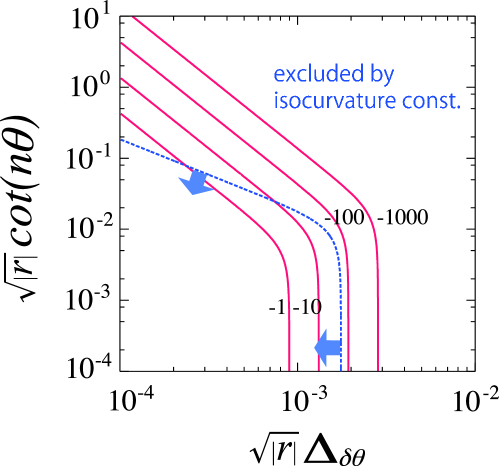
Figure 1: Contour of ${\rm sgn}(r)f_{\rm NL}^{\rm(iso)}=-1,-10,-100$ and $-1000$ (solid lines), together with the constraint on the isocurvature perturbation, $P_{S}/P_{\zeta}\mathop{}_{\textstyle\sim}^{\textstyle<}0.19$ (dotted line). The region above the constraint is excluded. We have set $n=6$ and approximated $\ln(kL)\sim 1$.

Lastly let us make a comment on a characteristic behavior of the baryonic isocurvature perturbations (29). The second order term , which represents the non-Gaussian perturbation, dominates over the linear fluctuation in the limit $\cot(n\theta)\to 0$. In this limit the baryon number itself created by the AD mechanism approaches to the maximum (see (26)). In Fig. 2 we show schematically the baryon asymmetry generated by the AD mechanism as a function of $\theta$. We have indicated the regions where $f_{\rm NL}^{\rm(iso)}$ is predicted to be positive or negative. This helps us understand why $f_{\rm NL}^{\rm(iso)}$ becomes negative when the positive baryon number is generated.

Figure 2: A schematic picture for the baryon asymmetry generated by the AD mechanism. We indicate the regions where $f_{\rm NL}^{\rm(iso)}$ is predicted to be positive or negative. Roughly speaking, the sign of $f_{\rm NL}^{\rm(iso)}$ is determined by the curvature of the curves, since the coefficient of the second order perturbations is determined by the second derivative of the baryon number.

III.1 Gravity-mediated SUSY breaking models

In gravity-mediation models, the whole potential of the AD field is given by Eqs. (21) and (22). In the following we assume $n=6$ . For simplicity, we do not consider the case that oscillation due to the thermal mass term occurs. This assumption is justified since we are interested in the regime $|\phi|\gg T$ to avoid the gravitino overproduction Moroi:1993mb ; Kawasaki:2004yh and hence particles that couple to the AD field cannot be thermalized. The AD field begins to oscillate due to thermal logarithmic term if the reheating temperature $T_{R}$ satisfies a condition (hereafter we take $a=1$),

$$\begin{split}T_{R}\;\gtrsim\;T_{R}^{c}&\;\equiv\;\frac{1}{\alpha}\left(\frac{m_{\phi}^{3}M^{3}}{M_{P}^{2}}\right)^{1/4}\\ &\;\sim\;1.1\times 10^{6}~{}{\rm GeV}\left(\frac{0.1}{\alpha}\right)\left(\frac{m_{\phi}}{1~{}{\rm TeV}}\right)^{3/4}\left(\frac{M}{10^{16}~{}{\rm GeV}}\right)^{3/4}.\end{split}$$ (38)

Otherwise it begins its oscillations by the soft mass term. Thus $r=n_{B}^{\rm(AD)}/n_{B}$ is estimated as

$$r\simeq\left\{\begin{array}[]{ll}0.27\displaystyle\left(\frac{m_{3/2}}{1~{}{\rm TeV}}\right)\left(\frac{T_{R}}{10^{4}~{}{\rm GeV}}\right)\left(\frac{1~{}{\rm TeV}}{m_{\phi}}\right)^{3/2}\left(\frac{M}{10^{16}~{}{\rm GeV}}\right)^{3/2}\sin(n\theta)&~{}~{}~{}{\rm for}~{}~{}~{}T_{R}<T_{R}^{c}\\ 0.35\displaystyle\left(\frac{0.1}{\alpha}\right)^{2}\left(\frac{m_{3/2}}{1~{}{\rm TeV}}\right)\left(\frac{10^{8}~{}{\rm GeV}}{T_{R}}\right)\left(\frac{M}{10^{16}~{}{\rm GeV}}\right)^{3}\sin(n\theta)&~{}~{}~{}{\rm for}~{}~{}~{}T_{R}>T_{R}^{c}\end{array}\right..$$ (39)

The CDM isocurvature perturbation $S$ is calculated as

$$S\simeq\left\{\begin{array}[]{ll}3\times 10^{-5}r^{1/2}\displaystyle\left(\frac{m_{3/2}}{1~{}{\rm TeV}}\right)^{1/2}\left(\frac{1~{}{\rm TeV}}{m_{\phi}}\right)^{3/4}\left(\frac{T_{R}}{10^{4}~{}{\rm GeV}}\right)^{1/2}\displaystyle\left(\frac{H_{\rm inf}}{10^{14}~{}{\rm GeV}}\right)^{3/4}\left(\frac{\cot(n\theta)}{10^{-2}}\right)\\ ~{}~{}~{}~{}~{}\times\sin^{1/2}(n\theta)~{}~{}~{}~{}~{}{\rm for}~{}~{}~{}T_{R}<T_{R}^{c}\\ 5\times 10^{-5}r^{3/4}\displaystyle\left(\frac{0.1}{\alpha}\right)^{1/2}\left(\frac{m_{3/2}}{1~{}{\rm TeV}}\right)^{1/4}\left(\frac{10^{8}~{}{\rm GeV}}{T_{R}}\right)^{1/4}\displaystyle\left(\frac{H_{\rm inf}}{10^{14}~{}{\rm GeV}}\right)^{3/4}\left(\frac{\cot(n\theta)}{10^{-2}}\right)\\ ~{}~{}~{}~{}~{}\times\sin^{1/4}(n\theta)~{}~{}~{}~{}~{}{\rm for}~{}~{}~{}T_{R}>T_{R}^{c}\end{array}\right.,$$ (40)

if the linear term in Eq. (29) dominates. This is constrained as $\Delta_{S}\lesssim 2.2\times 10^{-5}$ from WMAP5 results, as stated before. Then from Eq. (19) we can calculate $f_{\rm NL}^{\rm(iso)}$ as

$$f_{\rm NL}^{\rm(iso)}\simeq\left\{\begin{array}[]{ll}-2\times 10^{2}r\displaystyle\left(\frac{m_{3/2}}{1~{}{\rm TeV}}\right)^{2}\left(\frac{T_{R}}{10^{4}~{}{\rm GeV}}\right)^{2}\left(\frac{1~{}{\rm TeV}}{m_{\phi}}\right)^{3}\displaystyle\left(\frac{H_{\rm inf}}{10^{14}~{}{\rm GeV}}\right)^{3}\left(\frac{\cot(n\theta)}{10^{-2}}\right)^{2}\\ ~{}~{}~{}~{}~{}\times\sin^{2}(n\theta)~{}~{}~{}~{}~{}{\rm for}~{}~{}~{}T_{R}<T_{R}^{c}\\ -1\times 10^{3}r^{2}\displaystyle\left(\frac{0.1}{\alpha}\right)^{2}\left(\frac{m_{3/2}}{1~{}{\rm TeV}}\right)\left(\frac{10^{8}~{}{\rm GeV}}{T_{R}}\right)\displaystyle\left(\frac{H_{\rm inf}}{10^{14}~{}{\rm GeV}}\right)^{3}\left(\frac{\cot(n\theta)}{10^{-2}}\right)^{2}\\ ~{}~{}~{}~{}~{}\times\sin(n\theta)~{}~{}~{}~{}~{}{\rm for}~{}~{}~{}T_{R}>T_{R}^{c}\end{array}\right..$$ (41)

Thus depending on the sign of the CP phase ($\sin(n\theta)$) (or equivalently the baryon asymmetry), the non-linearity parameter can be either positive or negative.

Here we mention the effect of $Q$-ball formation. It is known that if a scalar field has a conserved global $U(1)$ charge  and if the scalar potential becomes flatter than a quadratic potential at larger field values, there exists a stable configuration of the scalar field, called $Q$-ball, whose stability is ensured by the $U(1)$ symmetry Coleman:1985ki . In the context of AD mechanism, this conserved $U(1)$ charge is the baryon number. In the AD mechanism, the scalar potential tends to be flatter than the quadratic term due to the renormalization group effects. Thus $Q$-balls are generically formed in the AD mechanism Kusenko:1997zq ; Dvali:1997qv ; Enqvist:1997si .

The charge of a $Q$-ball is given by

$$Q\;\simeq\;\gamma\left(\frac{\phi_{\rm os}}{m_{\phi}}\right)^{2}\times\left\{\begin{array}[]{ll}\epsilon{}{}{}&{\rm for}~{}~{}~{}\epsilon>\epsilon_{c}\\ \epsilon_{c}{}{}{}&{\rm for}~{}~{}~{}\epsilon<\epsilon_{c}\end{array}\right.,$$ (42)

where $\gamma\sim 6\times 10^{-3}$ and $\epsilon_{c}\sim 0.01$ from the lattice calculation Kasuya:1999wu . The parameter $\epsilon$ is called the ellipticity parameter, defined by the ratio of the minor and major axes of the orbit of the AD field $\phi$. It is roughly estimated as

$$\epsilon\;\sim\;\frac{m_{3/2}}{H_{\rm os}}\sin(n\theta).$$ (43)

If $Q\gg 10^{20}$, the decay temperature of the $Q$-ball becomes smaller than the freeze-out temperature of the lightest supersymmetric particle (LSP) and hence LSPs emitted by the $Q$-ball decay may be overproduced, depending on the self-annihilation cross section of the LSP Enqvist:1997si ; Fujii:2001xp ; Seto:2005pj ; Kawasaki:2007yy . The charge of the $Q$-ball, $Q$, is estimated as

$$Q\simeq\left\{\begin{array}[]{ll}2\times 10^{17}\displaystyle\left(\frac{m_{3/2}}{m_{\phi}}\right)\left(\frac{1~{}{\rm TeV}}{m_{\phi}}\right)^{3/2}\left(\frac{M}{10^{16}~{}{\rm GeV}}\right)^{3/2}~{}~{}~{}{\rm for}~{}~{}~{}T_{R}<T_{R}^{c}\\ 2\times 10^{11}\displaystyle\left(\frac{0.1}{\alpha}\right)^{2}\left(\frac{10^{8}~{}{\rm GeV}}{T_{R}}\right)^{2}\left(\frac{M}{10^{16}~{}{\rm GeV}}\right)^{3}~{}~{}~{}{\rm for}~{}~{}~{}T_{R}>T_{R}^{c}\end{array}\right..$$ (44)

If some fraction of LSP dark matter comes from the $Q$-ball decay, it produces the additional CDM isocurvature perturbation with some amount of non-Gaussianity. Furthermore, the decay rate of the $Q$-ball depends on its charge $Q$ and hence the decay rate also becomes the source for the isocurvature fluctuations Hamaguchi:2003dc as well as non-Gaussianity. However, in the interesting parameter regions, we have checked that the $Q$-balls evaporate in the high-temperature plasma and hence those effects of the $Q$-ball decay are negligible.

In Fig. 3 the contours of $f_{\rm NL}^{\rm(iso)}=-1$ and $-10$ are shown by the red solid and purple solid lines on the $(H_{\rm inf},T_{R})$ plane for $m_{3/2}=1$ TeV and $\cot(n\theta)=10^{-2}$. Here we have fixed $r=1$, i.e., the AD mechanism creates the total baryon asymmetry of the Universe. We also show the constraints from the isocurvature perturbation (green dashed), baryon overproduction (brown dot-dashed), gravitino overproduction (blue dotted), and LSP overproduction from $Q$-balls (orange long-dashed). To be conservative, we have estimated LSP abundance by neglecting the annihilation of the LSP, and we set the LSP mass to be 100 GeV. One can see that a significant amount of non-Gaussianity can be generated without conflicting the isocurvature constraint for the Hubble scale during inflation $H_{\rm inf}\gtrsim 10^{12}~{}$GeV. For $\cot(n\theta)\gtrsim 0.1$, the isocurvature constraint becomes more stringent and large $f_{\rm NL}^{\rm(iso)}$ cannot be generated without conflicting the isocurvature bound (see also Fig. 1).

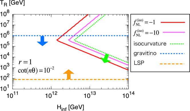
Figure 3: Constraints on $(H_{\rm inf},T_{R})$ for $m_{3/2}=1$ TeV and $\cot(n\theta)=10^{-2}$. We have fixed $r=1$. The lines show : $f_{\rm NL}^{\rm(iso)}=-1$ (red solid), $-10$ (purple solid), isocurvature bound (green dashed), gravitino overproduction bound (blue dotted), LSP overproduction from $Q$-ball decay (orange long-dashed). Arrows indicate the allowed region.

In the above arguments we have assumed that the AD mechanism provides the total baryon number of the Universe. However, the AD mechanism may create only small fraction of the baryon asymmetry, most of which is dominantly generated by another baryogenesis mechanism. In this case $r$ can be much smaller than unity. In Fig. 4 we similarly show the constraints on $(H_{\rm inf},T_{R})$ for $r=\pm 10^{-2}$, $m_{3/2}=1$ TeV and $\cot(n\theta)=10^{-2}$. If $r$ is positive (negative), $f_{\rm NL}^{\rm(iso)}$ becomes negative (positive). Thus large positive value of $f_{\rm NL}^{\rm(iso)}(\gtrsim 1)$ can be obtained if the AD mechanism creates small amount of baryon asymmetry with the negative sign. In this case the larger inflationary scale ($H_{\rm inf}\gtrsim 10^{13}$ GeV) than the case of $r=1$ is required (see Eq. (34)).

It may also be useful to rewrite Eqs. (40) and (41) by substituting (39),

$$S\simeq\left\{\begin{array}[]{ll}2\times 10^{-5}\displaystyle\left(\frac{m_{3/2}}{1~{}{\rm TeV}}\right)\left(\frac{T_{R}}{10^{4}~{}{\rm GeV}}\right)\left(\frac{1~{}{\rm TeV}}{m_{\phi}}\right)^{3/2}\left(\frac{M}{10^{16}~{}{\rm GeV}}\right)^{3/4}\displaystyle\left(\frac{H_{\rm inf}}{10^{14}~{}{\rm GeV}}\right)^{3/4}\left(\frac{\cot(n\theta)}{10^{-2}}\right)\\ ~{}~{}~{}~{}~{}\times\sin(n\theta)~{}~{}~{}~{}~{}{\rm for}~{}~{}~{}T_{R}<T_{R}^{c}\\ 2\times 10^{-5}\displaystyle\left(\frac{0.1}{\alpha}\right)^{2}\left(\frac{m_{3/2}}{1~{}{\rm TeV}}\right)\left(\frac{10^{8}~{}{\rm GeV}}{T_{R}}\right)\left(\frac{M}{10^{16}~{}{\rm GeV}}\right)^{9/4}\displaystyle\left(\frac{H_{\rm inf}}{10^{14}~{}{\rm GeV}}\right)^{3/4}\left(\frac{\cot(n\theta)}{10^{-2}}\right)\\ ~{}~{}~{}~{}~{}\times\sin(n\theta)~{}~{}~{}~{}~{}{\rm for}~{}~{}~{}T_{R}>T_{R}^{c}\end{array}\right.,$$ (45)

and

$$f_{\rm NL}^{\rm(iso)}\simeq\left\{\begin{array}[]{ll}-6\times 10^{1}\displaystyle\left(\frac{m_{3/2}}{1~{}{\rm TeV}}\right)^{3}\left(\frac{T_{R}}{10^{4}~{}{\rm GeV}}\right)^{3}\left(\frac{1~{}{\rm TeV}}{m_{\phi}}\right)^{9/2}\left(\frac{M}{10^{16}~{}{\rm GeV}}\right)^{3/2}\displaystyle\left(\frac{H_{\rm inf}}{10^{14}~{}{\rm GeV}}\right)^{3}\left(\frac{\cot(n\theta)}{10^{-2}}\right)^{2}\\ ~{}~{}~{}~{}~{}\times\sin^{3}(n\theta)~{}~{}~{}~{}~{}{\rm for}~{}~{}~{}T_{R}<T_{R}^{c}\\ -1\times 10^{2}\displaystyle\left(\frac{0.1}{\alpha}\right)^{6}\left(\frac{m_{3/2}}{1~{}{\rm TeV}}\right)^{3}\left(\frac{10^{8}~{}{\rm GeV}}{T_{R}}\right)^{3}\left(\frac{M}{10^{16}~{}{\rm GeV}}\right)^{6}\displaystyle\left(\frac{H_{\rm inf}}{10^{14}~{}{\rm GeV}}\right)^{3}\left(\frac{\cot(n\theta)}{10^{-2}}\right)^{2}\\ ~{}~{}~{}~{}~{}\times\sin^{3}(n\theta)~{}~{}~{}~{}~{}{\rm for}~{}~{}~{}T_{R}>T_{R}^{c}\end{array}\right..$$ (46)

We also show the constraints on $(M,T_{R})$ plane in Fig. 5 without fixing $r$. Here we take $m_{3/2}=1~{}$TeV, $\cot(n\theta)=10^{-2}$ and $H_{\rm inf}=10^{13}~{}$GeV. The red solid line shows $f_{\rm NL}^{\rm(iso)}=-1$. One can see that, for $|r|\leq 1$, the cutoff scale $M$ should be smaller than around $10^{16}~{}$GeV for generating large non-Gaussianity.

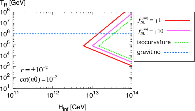
Figure 4: Same as Fig. 3, but for $r=\pm 10^{-2}$. The sign of $f_{\rm NL}^{\rm(iso)}$ depends on the sign of $r$.

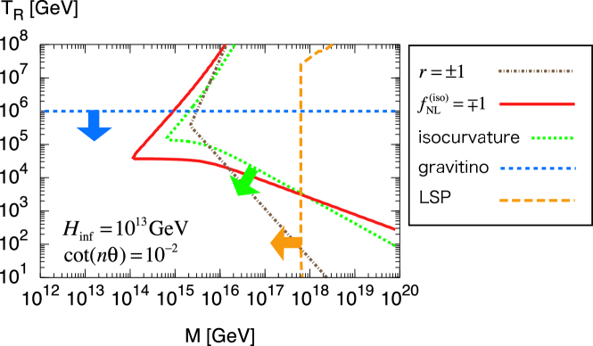
Figure 5: Constraints on $(M,T_{R})$ for $m_{3/2}=1$ TeV, $H_{\rm inf}=10^{13}~{}$GeV and $\cot(n\theta)=10^{-2}$. The lines show : $f_{\rm NL}^{\rm(iso)}=-1$ (red solid), isocurvature bound (green dashed), gravitino overproduction bound (blue dotted), baryon overproduction (brown dot-dashed) and LSP overproduction from $Q$-ball decay (orange long-dashed). Arrows indicate the allowed region.

III.2 Gauge-mediated SUSY breaking models

In gauge-mediated SUSY breaking models (GMSB) Giudice:1998bp , messenger fields mediate the SUSY breaking effect to the SSM sector. Here we assume the direct mediation scenario, that is, the SUSY breaking field $S$ couples to messenger fields ($\Psi,\bar{\Psi}$) in the superpotential as $W=S\Psi\bar{\Psi}$. In this type of models, the gauge mediation is suppressed for the scale $|\phi|\gtrsim\langle S\rangle$ where $\langle S\rangle$ is the vacuum expectation value of $S$. Instead there appears a logarithmic correction to the potential as de Gouvea:1997tn

$$\begin{split}V_{S}^{(\rm gauge)}(\phi)=&(m_{3/2}^{2}-cH^{2})|\phi|^{2}+V_{0}\left(\log\frac{|\phi|^{2}}{\langle S\rangle^{2}}\right)^{2}\\ &+\left(a_{m}m_{3/2}\frac{\phi^{n}}{nM^{n-3}}+{\rm h.c.}\right)+\frac{|\phi|^{2(n-1)}}{M^{2(n-3)}}~{}~{}~{}~{}~{}(|\phi|>\langle S\rangle),\end{split}$$ (47)

where $V_{0}$ is given by

$$V_{0}\equiv M_{F}^{4}=m_{\phi}^{2}\langle S\rangle^{2}\simeq\left(\frac{\alpha_{i}}{4\pi}\right)^{2}F_{S}^{2},$$ (48)

where $\alpha_{i}$ is the gauge couplings relevant for the AD field with $i$ denoting the gauge groups and $F_{S}=\sqrt{3}m_{3/2}M_{P}$ for vanishing cosmological constant. Thus the whole potential of the AD field is the sum of Eq. (22) and (47). The AD field begins to oscillate due to thermal logarithmic term for

$$\begin{split}T_{R}\;\gtrsim\;T_{R}^{c}&\equiv\frac{(MV_{0})^{3/10}}{\alpha M_{P}^{1/2}}\\ &\sim 5.3\times 10^{4}~{}{\rm GeV}\left(\frac{0.1}{\alpha}\right)\left(\frac{m_{3/2}}{1~{}{\rm MeV}}\right)^{3/5}\left(\frac{M}{10^{16}~{}{\rm GeV}}\right)^{3/10}.\end{split}$$ (49)

For $T_{R}<T_{R}^{c}$, the AD field begins to oscillate due to the logarithmic potential coming from the gauge mediation effects. The resultant baryon asymmetry can be estimated as

$$r\;\simeq\;\left\{\begin{array}[]{ll}1.3\times 10^{-4}\displaystyle\left(\frac{1~{}{\rm MeV}}{m_{3/2}}\right)^{1/5}\left(\frac{T_{R}}{10^{4}~{}{\rm GeV}}\right)\left(\frac{M}{10^{16}~{}{\rm GeV}}\right)^{12/5}\sin(n\theta)&~{}~{}~{}{\rm for}~{}~{}~{}T_{R}<T_{R}^{c}\\ 3.5\times 10^{-7}\displaystyle\left(\frac{0.1}{\alpha}\right)^{2}\left(\frac{m_{3/2}}{1~{}{\rm MeV}}\right)\left(\frac{10^{8}~{}{\rm GeV}}{T_{R}}\right)\left(\frac{M}{10^{16}~{}{\rm GeV}}\right)^{3}\sin(n\theta)&~{}~{}~{}{\rm for}~{}~{}~{}T_{R}>T_{R}^{c}\end{array}\right..$$ (50)

Thus the isocurvature perturbation is calculated as

$$S\;\simeq\;\left\{\begin{array}[]{ll}4\times 10^{-4}r^{11/16}\displaystyle\left(\frac{1~{}{\rm MeV}}{m_{3/2}}\right)^{1/16}\left(\frac{T_{R}}{10^{4}~{}{\rm GeV}}\right)^{5/16}\left(\frac{H_{\rm inf}}{10^{14}~{}{\rm GeV}}\right)^{3/4}\\ ~{}~{}~{}~{}~{}\times\cot(n\theta)\sin^{5/16}(n\theta)~{}~{}~{}{\rm for}~{}~{}~{}T_{R}<T_{R}^{c}\\ 2\times 10^{-4}r^{3/4}\displaystyle\left(\frac{0.1}{\alpha}\right)^{1/2}\left(\frac{m_{3/2}}{1~{}{\rm MeV}}\right)^{1/4}\left(\frac{10^{8}~{}{\rm GeV}}{T_{R}}\right)^{1/4}\left(\frac{H_{\rm inf}}{10^{14}~{}{\rm GeV}}\right)^{3/4}\\ ~{}~{}~{}~{}~{}\times\cot(n\theta)\sin^{1/4}(n\theta)~{}~{}~{}{\rm for}~{}~{}~{}T_{R}>T_{R}^{c}\end{array}\right.,$$ (51)

if the linear term in Eq. (29) dominates. The non-linearity parameter can be calculated as

$$f_{\rm NL}^{\rm(iso)}\;\simeq\;\left\{\begin{array}[]{ll}-5\times 10^{2}r^{7/4}\displaystyle\left(\frac{1~{}{\rm MeV}}{m_{3/2}}\right)^{1/4}\left(\frac{T_{R}}{10^{4}~{}{\rm GeV}}\right)^{5/4}\left(\frac{H_{\rm inf}}{10^{14}~{}{\rm GeV}}\right)^{3}\\ ~{}~{}~{}~{}~{}\times\cot^{2}(n\theta)\sin^{5/4}(n\theta)~{}~{}~{}{\rm for}~{}~{}~{}T_{R}<T_{R}^{c}\\ -1\times 10r^{2}\displaystyle\left(\frac{0.1}{\alpha}\right)^{2}\left(\frac{m_{3/2}}{1~{}{\rm MeV}}\right)\left(\frac{10^{8}~{}{\rm GeV}}{T_{R}}\right)\left(\frac{H_{\rm inf}}{10^{14}~{}{\rm GeV}}\right)^{3}\\ ~{}~{}~{}~{}~{}\times\cot^{2}(n\theta)\sin(n\theta)~{}~{}~{}{\rm for}~{}~{}~{}T_{R}>T_{R}^{c}\end{array}\right..$$ (52)

If the parameters take appropriate values, $f_{\rm NL}^{\rm(iso)}$ can be large enough with either positive or negative sign.

In GMSB models, there also exist a $Q$-ball solution, but its properties differ from those of the gravity-mediation type. The charge of the $Q$-ball is estimated as

$$Q\;\simeq\;\beta\left(\frac{\phi_{\rm os}}{M_{F}}\right)^{4}\times\left\{\begin{array}[]{ll}\epsilon{}{}{}&{\rm for}~{}~{}~{}\epsilon>\epsilon_{c}\\ \epsilon_{c}{}{}{}&{\rm for}~{}~{}~{}\epsilon<\epsilon_{c}\end{array}\right.,$$ (53)

where $\beta\sim 6\times 10^{-4}$ and $\epsilon_{c}\sim 0.06$ Kasuya:1999wu and $M_{F}$ in the denominator should be replaced with $T_{\rm os}$ if the oscillation begins due to thermal effects. If the $Q$-ball energy per unit charge ($M_{Q}/Q\sim M_{F}Q^{-1/4}$) is smaller than the nucleon mass $\sim 1$ GeV, $Q$-balls become stable against the decay into nucleons and contribute to some fraction of the dark matter Kusenko:1997si . Also in that case only the evaporated charges in the high-temperature plasma provides the baryon number remaining in the universe Laine:1998rg ; Banerjee:2000mb . In the regime of $\epsilon<\epsilon_{c}$ the $Q$-ball charge can be calculated as

$$Q\;\simeq\;\left\{\begin{array}[]{ll}5\times 10^{17}\displaystyle\left(\frac{1~{}{\rm MeV}}{m_{3/2}}\right)^{6/5}\left(\frac{M}{10^{16}~{}{\rm GeV}}\right)^{12/5}&~{}~{}~{}{\rm for}~{}~{}~{}T_{R}<T_{R}^{c}\\ 2\times 10^{11}\displaystyle\left(\frac{0.1}{\alpha}\right)^{2}\left(\frac{10^{8}~{}{\rm GeV}}{T_{R}}\right)^{2}\left(\frac{M}{10^{16}~{}{\rm GeV}}\right)^{3}&~{}~{}~{}{\rm for}~{}~{}~{}T_{R}>T_{R}^{c}\end{array}\right..$$ (54)

One can check that $1~{}$GeV $<M_{Q}/Q$ is always met in the parameter regions of our concern. Thus $Q$-balls are unstable in the most of the interesting parameter region and $Q$-ball formation does not affect following results. (Note that no LSPs are produced by the $Q$-ball decay since it is kinematically forbidden.)

Assuming that the AD mechanism creates the total baryon number of the Universe ($r=1$), we obtain constraints on $(H_{\rm inf},T_{R})$ plane as shown in Fig. 6. We have set $m_{3/2}=10$ GeV and $\cot(n\theta)=10^{-2}$. Meanings of lines are same as Fig. 3. We can see that a significant amount of non-Gaussianity can be generated, similar to the gravity-mediation case in the previous subsection. However, as we decrease the gravitino mass, the allowed region will become smaller.

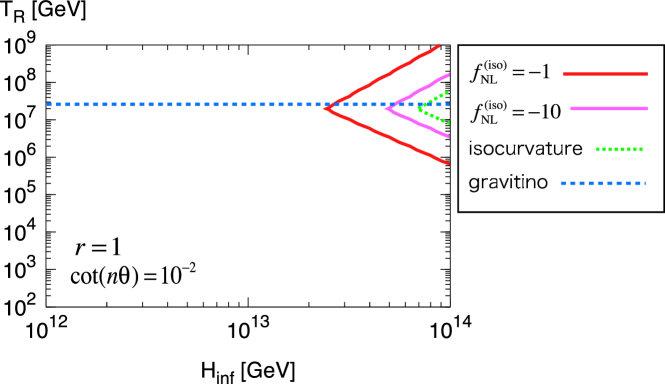
Figure 6: Same as Fig. 3, but for the gauge mediation. We have set $m_{3/2}=10$ GeV, $r=1$ and $\cot(n\theta)=10^{-2}$.

We are also interested in the case that the AD mechanism generates a small fraction of the baryon asymmetry, with both positive and negative signs. Substituting (50) into Eqs. (51) and (52) yields

$$S\simeq\left\{\begin{array}[]{ll}8\times 10^{-7}\displaystyle\left(\frac{1~{}{\rm MeV}}{m_{3/2}}\right)^{1/5}\left(\frac{T_{R}}{10^{4}~{}{\rm GeV}}\right)\left(\frac{M}{10^{16}~{}{\rm GeV}}\right)^{33/20}\left(\frac{H_{\rm inf}}{10^{14}~{}{\rm GeV}}\right)^{3/4}\\ ~{}~{}~{}~{}~{}\times\cot(n\theta)\sin(n\theta)~{}~{}~{}{\rm for}~{}~{}~{}T_{R}<T_{R}^{c}\\ 2\times 10^{-9}\displaystyle\left(\frac{0.1}{\alpha}\right)^{2}\left(\frac{m_{3/2}}{1~{}{\rm MeV}}\right)\left(\frac{10^{8}~{}{\rm GeV}}{T_{R}}\right)\left(\frac{M}{10^{16}~{}{\rm GeV}}\right)^{9/4}\left(\frac{H_{\rm inf}}{10^{14}~{}{\rm GeV}}\right)^{3/4}\\ ~{}~{}~{}~{}~{}\times\cot(n\theta)\sin(n\theta)~{}~{}~{}{\rm for}~{}~{}~{}T_{R}>T_{R}^{c}\end{array}\right..$$ (55)

and

$$f_{\rm NL}^{\rm(iso)}\simeq\left\{\begin{array}[]{ll}-9\times 10^{-5}\displaystyle\left(\frac{1~{}{\rm MeV}}{m_{3/2}}\right)^{3/5}\left(\frac{T_{R}}{10^{4}~{}{\rm GeV}}\right)^{3}\left(\frac{M}{10^{16}~{}{\rm GeV}}\right)^{21/5}\left(\frac{H_{\rm inf}}{10^{14}~{}{\rm GeV}}\right)^{3}\\ ~{}~{}~{}~{}~{}\times\cot^{2}(n\theta)\sin^{3}(n\theta)~{}~{}~{}{\rm for}~{}~{}~{}T_{R}<T_{R}^{c}\\ -1\times 10^{-12}\displaystyle\left(\frac{0.1}{\alpha}\right)^{6}\left(\frac{m_{3/2}}{1~{}{\rm MeV}}\right)^{3}\left(\frac{10^{8}~{}{\rm GeV}}{T_{R}}\right)^{3}\left(\frac{M}{10^{16}~{}{\rm GeV}}\right)^{6}\left(\frac{H_{\rm inf}}{10^{14}~{}{\rm GeV}}\right)^{3}\\ ~{}~{}~{}~{}~{}\times\cot^{2}(n\theta)\sin^{3}(n\theta)~{}~{}~{}{\rm for}~{}~{}~{}T_{R}>T_{R}^{c}\end{array}\right..$$ (56)

The resultant constraints are shown in Fig. 7 on $(M,T_{R})$ plane. We have set $m_{3/2}=10~{}$GeV, $H_{\rm inf}=10^{14}$ GeV and $\cot(n\theta)=10^{-2}$. We can see that either positive or negative $f_{\rm NL}^{\rm(iso)}$ can be obtained through the AD mechanism while satisfying the isocurvature constraint.

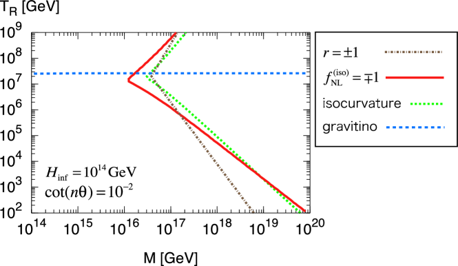
Figure 7: Same as Fig. 5, but for the gauge mediation. We have set $m_{3/2}=10$ GeV, $H_{\rm inf}=10^{14}~{}$GeV and $\cot(n\theta)=10^{-2}$.

IV Discussion and Conclusions

We have focused on the AD mechanism in this paper, but there are other baryogenesis scenarios that may induce large non-Gaussianity in the baryon asymmetry. For instance, it is known that the spontaneous baryogenesis Cohen:1988kt can lead to the baryonic isocurvature perturbations, since in the original model a non-vanishing chemical potential is due to a slow-rolling scalar field. In order to estimate non-Gaussianity, however, one has to specify how the chemical potential for the baryon number arises. In the case of the spontaneous baryogenesis using a flat direction of the SSM Chiba:2003vp , the resultant non-Gaussianity has almost the same features as that in the case of the AD mechanism. Another example is non-thermal leptogenesis using the right-handed sneutrino condensate, $\tilde{N}$ Murayama:1993em . Suppose that $\tilde{N}$ is light and fluctuating around the origin during inflation. Such a set-up may occur without fine-tuning, because the origin is the symmetry-enhanced point, and this is exactly what is considered in the ungaussiton scenario Suyama:2008nt . The $\tilde{N}$ can generate non-Gaussianity in both the adiabatic and baryonic isocurvature perturbations. If the mass of the right-handed sneutrino is heavy, the baryonic isocurvature perturbations will become more important than the adiabatic one. In this scenario, the non-Gaussianity becomes large only if the non-thermal leptogenesis accounts for a tiny fraction of the baryon asymmetry.

It is also possible to consider non-Gaussianity in other type of isocurvature perturbations. For instance, a large lepton asymmetry may have isocurvature perturbations with some amount of non-Gaussianity. If they are generated by the AD field with a lepton number Kawasaki:2002hq , non-Gaussianity arises from the fluctuations of the phase component, as in the case of the AD mechanism. However, such isocurvature perturbations will affect the CMB temperature fluctuations in a different way, and so does the associated non-Gaussianity. We leave this issue for future work.

So far we have considered up to the three-point correlation functions. It is straightforward to extend our analysis to the correlation functions of higher order. In particular, when the linear perturbation is negligible, we have a consistency relation between $f_{\rm NL}$ and $\tau_{\rm NL}$ as in the case of the ungaussiton Suyama:2008nt , the latter of which is defined as a non-linearity parameter of the four-point correlation function.

In summary, in this paper we have studied a scenario that non-Gaussian baryonic isocurvature fluctuation is produced from the AD mechanism in SUSY. We have found that the AD mechanism can create large non-Gaussianity without conflicting with the current isocurvature constraint. We have seen that for $|f_{\rm NL}^{\rm(iso)}|\gtrsim 1$ the Hubble parameter during inflation must be larger than about $10^{12}$ GeV, and that $|f_{\rm NL}^{\rm(iso)}|$ is bounded as $|f_{\rm NL}^{\rm(iso)}|<60$ to satisfy the isocurvature constraint. Interestingly, as opposed to many known mechanisms for generating sizable non-Gaussianity , the AD field can generate large non-Gaussianity even if it is the main component for generating the baryon asymmetry. The non-linerity parameter $f_{\rm NL}^{\rm(iso)}$ is negative if the AD mechanism is responsible for the total baryon asymmetry of the Universe, while it can be either positive or negative otherwise.

In our scenario the non-Gaussianity is necessarily accompanied with some amount of the isocurvature perturbations, therefore, if there are indeed large non-Gaussianity arising from the isocurvature perturbations, the future (or even on-going) observations will detect the isocurvature perturbations. It would be very interesting if the non-Gaussianity tells us about the origin of the baryon asymmetry, which is difficult to be probed, otherwise.

- (1) E. Komatsu et al. [WMAP Collaboration], arXiv:0803.0547 [astro-ph].
- (2) A. P. S. Yadav and B. D. Wandelt, Phys. Rev. Lett. 100, 181301 (2008) [arXiv:0712.1148 [astro-ph]].
- (3) D. H. Lyth and D. Wands, Phys. Lett. B 524, 5 (2002) [arXiv:hep-ph/0110002]; T. Moroi and T. Takahashi, Phys. Lett. B 522, 215 (2001) [Erratum-ibid. B 539, 303 (2002)] [arXiv:hep-ph/0110096]; K. Enqvist and M. S. Sloth, Nucl. Phys. B 626, 395 (2002) [arXiv:hep-ph/0109214].
- (4) D. H. Lyth, C. Ungarelli and D. Wands, Phys. Rev. D 67, 023503 (2003) [arXiv:astro-ph/0208055].
- (5) T. Suyama and F. Takahashi, arXiv:0804.0425 [astro-ph].
- (6) A. D. Linde and V. F. Mukhanov, Phys. Rev. D 56, 535 (1997) [arXiv:astro-ph/9610219].
- (7) L. Boubekeur and D. H. Lyth, Phys. Rev. D 73, 021301 (2006) [arXiv:astro-ph/0504046].
- (8) M. Kawasaki, K. Nakayama, T. Sekiguchi, T. Suyama and F. Takahashi, arXiv:0808.0009 [astro-ph]; arXiv:0810.0208 [astro-ph].
- (9) I. Affleck and M. Dine, Nucl. Phys. B 249, 361 (1985).
- (10) M. Dine, L. Randall and S. D. Thomas, Nucl. Phys. B 458, 291 (1996) [arXiv:hep-ph/9507453].
- (11) S. R. Coleman, Nucl. Phys. B 262, 263 (1985) [Erratum-ibid. B 269, 744 (1986)].
- (12) A. Kusenko, Phys. Lett. B 405, 108 (1997) [arXiv:hep-ph/9704273]; Phys. Lett. B 404, 285 (1997) [arXiv:hep-th/9704073].
- (13) G. R. Dvali, A. Kusenko and M. E. Shaposhnikov, Phys. Lett. B 417, 99 (1998) [arXiv:hep-ph/9707423].
- (14) K. Enqvist and J. McDonald, Phys. Lett. B 425, 309 (1998) [arXiv:hep-ph/9711514]; Nucl. Phys. B 538, 321 (1999) [arXiv:hep-ph/9803380]; Nucl. Phys. B 570, 407 (2000) [arXiv:hep-ph/9908316]; K. Enqvist, A. Jokinen and J. McDonald, Phys. Lett. B 483, 191 (2000) [arXiv:hep-ph/0004050].
- (15) A. D. Linde, Phys. Lett. B 160, 243 (1985).
- (16) K. Enqvist and J. McDonald, Phys. Rev. Lett. 83, 2510 (1999) [arXiv:hep-ph/9811412]; Phys. Rev. D 62, 043502 (2000) [arXiv:hep-ph/9912478]; M. Kawasaki and F. Takahashi, Phys. Lett. B 516, 388 (2001) [arXiv:hep-ph/0105134].
- (17) S. Kasuya, M. Kawasaki and F. Takahashi, arXiv:0805.4245 [hep-ph].
- (18) D. Babich, P. Creminelli and M. Zaldarriaga, JCAP 0408, 009 (2004) [arXiv:astro-ph/0405356].
- (19) D. H. Lyth, Phys. Rev. D 45, 3394 (1992).
- (20) D. H. Lyth, JCAP 0712, 016 (2007) [arXiv:0707.0361 [astro-ph]].
- (21) T. Gherghetta, C. F. Kolda and S. P. Martin, Nucl. Phys. B 468, 37 (1996) [arXiv:hep-ph/9510370].
- (22) R. Allahverdi, B. A. Campbell and J. R. Ellis, Nucl. Phys. B 579, 355 (2000) [arXiv:hep-ph/0001122].
- (23) A. Anisimov and M. Dine, Nucl. Phys. B 619, 729 (2001) [arXiv:hep-ph/0008058].
- (24) S. Kasuya, M. Kawasaki and F. Takahashi, Phys. Lett. B 578, 259 (2004) [arXiv:hep-ph/0305134].
- (25) S. Kasuya, M. Kawasaki and F. Takahashi, Phys. Rev. D 68, 023501 (2003) [arXiv:hep-ph/0302154].
- (26) M. Fujii, K. Hamaguchi and T. Yanagida, Phys. Rev. D 63, 123513 (2001) [arXiv:hep-ph/0102187]; M. Kawasaki and K. Nakayama, JCAP 0702, 002 (2007) [arXiv:hep-ph/0611320].
- (27) A. Riotto and F. Riva, arXiv:0806.3382 [hep-ph].
- (28) T. Moroi, H. Murayama and M. Yamaguchi, Phys. Lett. B 303, 289 (1993).
- (29) M. Kawasaki, K. Kohri and T. Moroi, Phys. Lett. B 625, 7 (2005) [arXiv:astro-ph/0402490]; Phys. Rev. D 71, 083502 (2005) [arXiv:astro-ph/0408426]; M. Kawasaki, K. Kohri, T. Moroi and A. Yotsuyanagi, arXiv:0804.3745 [hep-ph].
- (30) M. Kawasaki, K. Konya and F. Takahashi, Phys. Lett. B 619, 233 (2005) [arXiv:hep-ph/0504105].
- (31) S. Kasuya and M. Kawasaki, Phys. Rev. D 61, 041301 (2000) [arXiv:hep-ph/9909509]; Phys. Rev. D 64, 123515 (2001) [arXiv:hep-ph/0106119].
- (32) M. Fujii and K. Hamaguchi, Phys. Lett. B 525, 143 (2002) [arXiv:hep-ph/0110072]; Phys. Rev. D 66, 083501 (2002) [arXiv:hep-ph/0205044]; M. Fujii and T. Yanagida, Phys. Lett. B 542, 80 (2002) [arXiv:hep-ph/0206066].
- (33) O. Seto, Phys. Rev. D 73, 043509 (2006) [arXiv:hep-ph/0512071].
- (34) M. Kawasaki and K. Nakayama, Phys. Rev. D 76, 043502 (2007) [arXiv:0705.0079 [hep-ph]].
- (35) K. Hamaguchi, M. Kawasaki, T. Moroi and F. Takahashi, Phys. Rev. D 69, 063504 (2004) [arXiv:hep-ph/0308174].
- (36) For a review, see G. F. Giudice and R. Rattazzi, Phys. Rept. 322, 419 (1999) [arXiv:hep-ph/9801271].
- (37) A. de Gouvea, T. Moroi and H. Murayama, Phys. Rev. D 56, 1281 (1997) [arXiv:hep-ph/9701244].
- (38) A. Kusenko and M. E. Shaposhnikov, Phys. Lett. B 418, 46 (1998) [arXiv:hep-ph/9709492].
- (39) M. Laine and M. E. Shaposhnikov, Nucl. Phys. B 532, 376 (1998) [arXiv:hep-ph/9804237].
- (40) R. Banerjee and K. Jedamzik, Phys. Lett. B 484, 278 (2000) [arXiv:hep-ph/0005031].
- (41) A. G. Cohen and D. B. Kaplan, Nucl. Phys. B 308, 913 (1988); A. G. Cohen, D. B. Kaplan and A. E. Nelson, Phys. Lett. B 263, 86 (1991).
- (42) T. Chiba, F. Takahashi and M. Yamaguchi, Phys. Rev. Lett. 92, 011301 (2004) [arXiv:hep-ph/0304102]; F. Takahashi and M. Yamaguchi, Phys. Rev. D 69, 083506 (2004) [arXiv:hep-ph/0308173].
- (43) M. Kawasaki, F. Takahashi and M. Yamaguchi, Phys. Rev. D 66, 043516 (2002) [arXiv:hep-ph/0205101].
- (44) H. Murayama and T. Yanagida, Phys. Lett. B 322, 349 (1994) [arXiv:hep-ph/9310297]; K. Hamaguchi, H. Murayama and T. Yanagida, Phys. Rev. D 65, 043512 (2002) [arXiv:hep-ph/0109030].
- (45) K. Enqvist and T. Takahashi, arXiv:0807.3069 [astro-ph]; Q. G. Huang and Y. Wang, arXiv:0808.1168 [hep-th].