Tunable Spin Filtering through an Aluminum Nanoparticle

Abstract

Spin-polarized current through an Al nanoparticle in tunnel contact with two ferromagnets is measured as a function of the direction of the applied magnetic field. The nanoparticle filters the spin of injected electrons along a direction specified by the magnetic field. The characteristic field scale for the filtering corresponds to a lower limit of $8ns$ for the spin-dephasing time. Spin polarized current versus applied voltage increases stepwise, confirming that the spin relaxation time is long only in the ground state and the low-lying excited states of the nanoparticle.

To study and manipulate the properties of the electron spin in a quantum dot and other electronic structures remains a challenge. The injection, detection, and coherent manipulation of the electron spin in GaAs quantum dots have been reported recently. Petta et al. (2004); Koppens et al. (2006) At room temperature, spin injection, detection, and precession have been measured in mesoscopic Al strips coupled to ferromagnets by tunnel contacts. Jedema et al. (2001) The dephasing time of the precession is comparable to the electron spin-orbit scattering time $\tau_{SO}\sim 10^{-10}$s.

In metallic nanoparticles, quantum dot behavior persists at higher temperatures than in semiconducting quantum dots, making it relevant to explore spin-relaxation and dephasing in this system. We expect much longer spin dephasing times in Al nanoparticles compared to mesoscopic strips because of the finite size effect. When the sample size is reduced, both $1/\tau_{SO}$ and the electron-in-a-box level spacing $\delta$ increase, but $\delta$ increases much faster than $1/\tau_{SO}$. Wei et al. (2008) If the nanoparticles diameter is $D<10nm$, then $\delta>\hbar/\tau_{SO}$, Wei et al. (2008) and the effects of spin-orbit scattering are suppressed. Salinas et al. (1999); Brouwer et al. (2000); Matveev et al. (2000) Evidence of long spin-relaxation time in metallic nanoparticles have been reported. Bernand-Mantel et al. (2006); Wei et al. (2007); Mitani et al. (2008) As will be shown, we can set a lower limit for the dephasing time in our sample of 8 ns.

Here we report measurements of spin injection, detection, and basic spin manipulation performed at 4.2 K in an Al nanoparticle coupled to two ferromagnets by tunnel contacts. The nanoparticle serves as a quantum dot. The injection and detection of spins is provided by two ferromagnets, while the manipulation is to filter, e.g. to project, the spin of injected electrons along the direction specified by the applied magnetic field. The idea to use metallic nanoparticle states as spin-filters to study the magnetization in the ferromagnetic leads was introduced in Ref. Deshmukh and Ralph (2002) Here we are interested in that filtering to study the properties of the spin in the nanoparticle, such as dephasing. Spin filtering using ferromagnetic tunnel barriers have been studied recently, Santos and Moodera (2004); Gajek et al. (2005); Ramos et al. (2007) to inject spins into normal metals without ferromagnetic source and drain leads. As will be shown, in metallic nanoparticles, the magnetic field scale for spin filtering is very small, providing tunable control of the spin direction.

To understand how a magnetic field $\vec{B}$ influences the spin-polarized current through the nanoparticle, we consider electron transport via Zeeman split electron-in-a-box energy levels. In the ferromagnets, electrons move in an exchange field oriented along the z-axis, so the spinors are $|\uparrow>$ and $|\downarrow>$. In the nanoparticle, the exchange field is negligible, because the tunnel barriers in our samples are assumed to be very thick, and the Zeeman splitting in $\vec{B}$ defines spinors $|\uparrow^{\prime}>$ and $|\downarrow^{\prime}>$.

We obtain the tunnel-rate $\Gamma_{|\uparrow^{\prime}>}^{r}(\alpha)$ between lead $r$ ($r=R,L$) and an electron-in-a-box level with spin $|\uparrow^{\prime}>$ as a function of angle $\alpha$ between $\vec{B}$ and the z-axis, as sketched in Fig. 1. The magnetization direction is indicated by parameter $\sigma=\pm 1$ for up and down directions, respectively. We use a spinor transformation $|\uparrow^{\prime}>=cos(\alpha/2)|\uparrow>+sin(\alpha/2)|\downarrow>$, and consider continuity of the wavefunction at the ferromagnet interface. With that boundary condition, the tunnel rate between $|\uparrow^{\prime}>$ and the $|\uparrow>$-band in the ferromagnets is reduced proportionally by a factor of  Slonczewski (1989) $cos^{2}(\alpha/2)$. That tunnel rate can be expressed as $\Gamma^{r}(1+\sigma P)cos^{2}(\alpha/2)$, where $\Gamma^{r}$ is the bare tunnel rate defined in Ref. Wei et al. (2008) and $P$ is the spin-polarization in the tunnel density of states in the leads.

If $\alpha\neq 0$, there is also a nonzero transmission between $|\uparrow^{\prime}>$ and the spin-down band. Following a similar analysis as that above, the tunnel rate between $|\uparrow^{\prime}>$ and the spin-down band is $\Gamma^{r}(1-\sigma P)sin^{2}(\alpha/2)$. The total tunnel rate between $|\uparrow^{\prime}>$ and lead $r$ is obtained by summing over the spin-bands: $\Gamma_{|\uparrow^{\prime}>}^{r}(\alpha)=\Gamma^{r}[1+\sigma Pcos(\alpha)]$. Similarly, the total tunnel rate between $|\downarrow^{\prime}>$ and lead $r$ is $\Gamma_{|\downarrow^{\prime}>}^{r}(\alpha)=\Gamma^{r}[1-\sigma Pcos(\alpha)]$.

Overall, $\vec{B}$ effectively changes the spin-polarization in the leads from $P$ to $Pcos(\alpha)$. One can obtain the $\vec{B}$-dependence of the current using models of spin-polarized current through the nanoparticle in zero field, by substituting $P$ with $Pcos(\alpha)$.

The spin-polarized current through the nanoparticle is mediated by spin accumulation. Brataas et al. (1999); Weymann et al. (20053); Braun et al. (2004) Spin accumulation occurs when the nanoparticle internally excited states with one spin direction, generated by electron tunnelling and sketched in Fig. 1-A, have higher probability compared to the states with reversed spin direction.

In the parallel magnetic configuration, $\Gamma_{|\uparrow^{\prime}>}^{L}(\alpha)/\Gamma_{|\uparrow^{\prime}>}^{R}(\alpha)=\Gamma_{|\downarrow^{\prime}>}^{L}(\alpha)/\Gamma_{|\downarrow^{\prime}>}^{R}(\alpha)$, and sequential electron tunnelling through the nanoparticle will not cause spin accumulation. In that case $I_{\uparrow\uparrow}$ versus $\vec{B}$ is constant. This should be contrasted with the Hanle effect in mesoscopic spin valves, Johnson and Silsbee (1985) where $I_{\uparrow\uparrow}$ versus $B_{\perp}$ exhibits a maximum at $B_{\perp}=0$.

In the antiparallel magnetic state, where $\sigma=1$ and $-1$ for leads $L$ and $R$, respectively, $\Gamma_{|\uparrow^{\prime}>}^{L}(\alpha)/\Gamma_{|\uparrow^{\prime}>}^{R}(\alpha)>\Gamma_{|\downarrow^{\prime}>}^{L}(\alpha)/\Gamma_{|\downarrow^{\prime}>}^{R}(\alpha)$. In that case, sequential electron tunnelling through the nanoparticle will cause spin accumulation. Using the spin-accumulation model in our prior work Wei et al. (2008) and substituting $P$ with $Pcos(\alpha)$, we obtain

$$\Delta I(\alpha)=\Delta I(0)cos^{2}(\alpha)=\Delta I(0)\frac{B_{z}^{2}}{B_{\perp}^{2}+B_{z}^{2}}$$ (1)

where $\Delta I(\alpha)=I_{\uparrow\uparrow}-I_{\uparrow\downarrow}(\alpha)$ is the difference in the current between the parallel and the antiparallel magnetic configuration. This equation will be referred to as the spin-filter model.

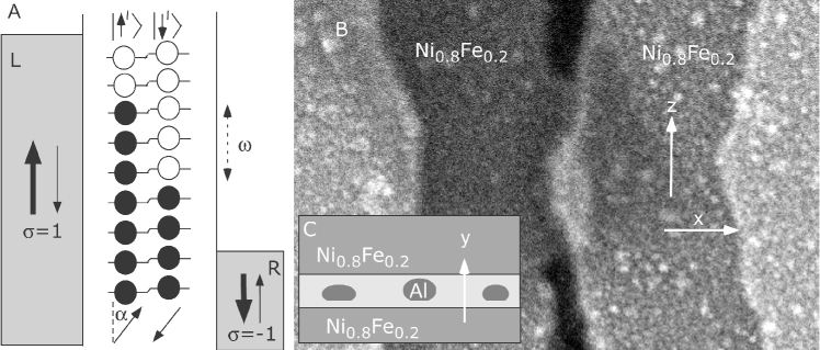
Figure 1: A: An excited state of the nanoparticle generated at finite bias voltage, fully relaxed with respect to spin-conserving transitions. Filled circles indicate occupied electron-in-a-box states. The spin expectation value is tilted by the magnetic field. B: Electron microscope image of a typical device. C: Sketch of the tunnel junction cross-section.

Our typical device is shown in Fig. 1-B. An $Al_{2}O_{3}$ tunnel junction is sandwiched between two $Ni80Fe20$ leads in the overlap region in the center. Al nanoparticles are embedded in the tunnel junction, as sketched in Fig. 1-C. Many devices are made simultaneously with variable size of the overlap region, which varies from a large value to zero. We select the devices at the threshold of electric conduction, which significantly enhances the chance that the current between the leads flows via a single nanoparticle. Wei et al. (2007) The arrangement of the leads favors antiparallel magnetic directions. The details of the fabrication are explained in Ref. Wei et al. (2007)

At 4.2K, the samples exhibit Coulomb-Blockade (CB). Among the selected samples, typical parameters are $D\approx 5nm$, $\delta\sim 1meV$, and $\Gamma\sim MHz$, where $\Gamma$ is the tunnel rate between the discrete levels and the leads. The spin-conserving energy relaxation rate in these conditions is $\gg\Gamma$. At a bias voltage larger than the CB-threshold, only those nanoparticle states that are fully relaxed with respect to spin-conserving transitions have significant probability in the ensemble of excited states generated by tunnelling. One such excited state is displayed in Fig. 1-A.

Fig. 2-A displays the I-V curve of one device at 4.2K. The I-V curve exhibits CB. In addition to the conduction thresholds indicated by the letters a and b, there are thresholds at higher bias voltages where the slope of the I-V curve increases sharply, as indicated by the letter c at positive voltage. At the threshold voltages, additional charged states of the nanoparticle become energetically available for tunneling, consistent with CB. Averin and Likharev (1991)

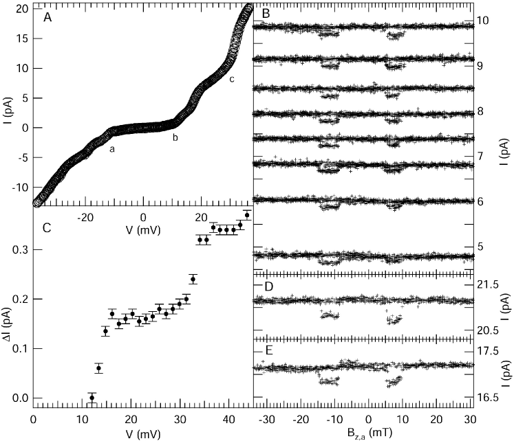
Figure 2: A: I-V curve. B: $I$ versus $B_{z,a}$, with increasing bias voltage. C: $\Delta I=I_{\uparrow\uparrow}-I_{\uparrow\downarrow}$ versus $V$. D and E: $I$ versus $B_{z,a}$ at $V=35mV$ and $V=40mV$, respectively. All data taken at $T=4.2K$.

Current versus parallel applied field $B_{z,a}$ is displayed in Fig. 2-B. There are 8 dependencies shown, each obtained at a different bias voltage. The bias voltage varies by 1.4mV between successive dependencies. At each bias voltage, the field sweeps four times in the positive and negative field directions.

The dependencies signal the spin-valve effect. There are two pairs of magnetic transitions, one for each sweep direction. In a magnetic transition, the magnetic configuration switches between parallel and antiparallel, resulting in the current change $\Delta I=I_{\uparrow\uparrow}-I_{\uparrow\downarrow}$.

In Fig. 2-B, $\Delta I\approx 0.17pA$ is evidently independent of $V$. $\Delta I$ versus $V$ is shown explicitly in Fig. 2-C. From $V=0$ to $V=32mV$, $\Delta I$ clearly displays saturation. We also measure the spin-valve signals at negative bias voltage, and find the same behavior in $\Delta I$ versus $V$, with the same magnitude of $\Delta I$.

The saturation of $\Delta I$ versus $V$ has been reported in our previous work. Wei et al. (2007, 2008) $\Delta I$ versus $V$ typically saturates within the first two or three discrete energy levels available for tunnelling above the CB-threshold. The saturation was explained by a rapid decrease in $T_{1}$ versus energy difference $\omega$ in a spin-flip transition. To summarize, at low bias voltage, where $1/T_{1}(\omega)<\Gamma$ for any excitation energy $\omega$, $\Delta I\approx cI_{\uparrow\uparrow}$, where $c$ is on the order of $2P^{2}$ (the Julliere’s value). As the voltage increases, the range of $\omega$ increases and $\Delta I$ saturates roughly when there is an $\omega$ for which $1/T_{1}(\omega)\sim\Gamma$. Self-consistent calculation of the saturation parameters can be done using a model in Ref. Wei et al. (2008), which have lead to an estimate $T_{1}(\delta)\approx 1\mu s$.

Unexpectedly, $\Delta I$ versus $V$ in Fig. 2-C exhibits another increase at $V\approx 32mV$. The dependencies $I$ versus $B_{z}$ at $V>32mV$ are shown in Fig. 2-D and E. $\Delta I$ in these figures is approximately two times larger than $\Delta I$ in Fig. 2-B. To our knowledge, the data in Fig. 2B-E is the first observation of a stepwise increase of the spin-polarized current with bias voltage through a quantum dot.

The increase in $\Delta I$ occurs at the conduction threshold voltage c in Fig. 2-A. At that voltage, an additional charged state becomes energetically available for electron tunneling and starts to contribute significantly to electron transport. So, the addition of a charged state effectively adds a channel for spin-accumulation and spin-polarized transport.

At the threshold where the additional charged state becomes energetically available, there is insufficient energy to generate internally excited states in the nanoparticle in that additional charged state. In that case the nanoparticle in the additional charged state must be in the ground state. If the voltage is slightly larger than the threshold voltage, then the internal excitation energy $\omega$ in the additional charged state will be small and the condition $1/T_{1}(\omega)<\Gamma$ will be satisfied again, leading to spin-accumulation. The observation of the step-wise increase in $\Delta I$ demonstrates the correctness of our interpretation of the saturation effect in terms of $T_{1}(\omega)$ dependence, strengthening our case that we measured the spin-relaxation time in prior work. Wei et al. (2007, 2008)

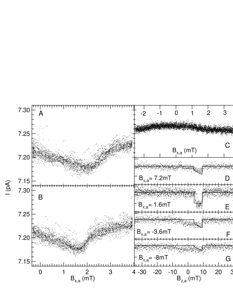
Figure 3: A and B: $I_{\uparrow\downarrow}$ versus $B_{x,a}$, for increasing and decreasing $B_{x,a}$, respectively, at $B_{y,a}=B_{z,a}=0$. C: $I_{\uparrow\uparrow}$ versus $B_{x,a}$, at $B_{y,a}=B_{z,a}=0$. D-G: Suppression of the spin-valve signal with perpendicular applied field. T=4.2K in all figures.

Now we investigate how a perpendicular field influences spin-polarized current through the nanoparticle. The magnetizations are set into the antiparallel configuration using the spin-valve signal and then the applied field is reduced to zero. Figs. 3-A and B display current versus magnetic field $B_{x,a}$ applied along the $x$-axis, when the magnetic field is sweeping up and down, respectively. The $x$-axis is indicated in Fig. 1-B. The components of the applied magnetic field along the easy and the hard axes are zero.

We have carefully measured current versus $B_{x,a}$ in the parallel magnetic configuration, when $B_{z,a}=B_{y,a}=0$. The results are shown in Fig. 3-C. Comparing Figs. 3-A, B, and C, it is concluded that $I$ versus $B_{x,a}$ exhibits a minimum in the antiparallel magnetic configuration and $I$ versus $B_{x,a}$ is constant in the parallel magnetic configuration.

The minimum center is offset and the amplitude of the minimum, $\approx 0.05pA$, is smaller than $\Delta I=0.17pA$ measured in the spin-valve signal in Fig. 2. Comparing Figs. 3-A and B, we conclude that the minimum is reversible with magnetic field, although there is a weak hysteresis, of approximately $0.2mT$.

The spin-valve signal is suppressed with the applied perpendicular field, as shown in Figs. 3-D, E, F, and G. The strongest spin-valve signal, shown in Fig. 3-E, is measured around the perpendicular field at the minimum of Figs. 3-A and B. In a strong perpendicular field, Fig. 3-D,F, and G, the magnetic transitions from parallel into antiparallel magnetic state become significantly weakened; as $B_{z,a}$ approaches the magnetic transition from antiparallel into the parallel magnetic state, there is now a gradual decrease in current. The transitions from antiparallel to parallel magnetic state in a strong perpendicular field remain resolved, but they are weakened proportionally to the magnitude of the perpendicular field. The characteristic perpendicular field that weakens the spin-valve signal is much larger than the width of the minimum in Fig. 3-A and B.

The measurements are in agreement with the spin-filter model described in the introduction. We must rule out a possibility that the dependencies in Figs. 3 are caused by rotation of the magnetizations in response to the perpendicular field as it could explain the data so far presented. Starting from the antiparallel magnetic configuration, a rotation would vary the magnetizations from antiparallel to parallel, leading to a minimum in $I$ versus $B_{x,a}$. Starting from the parallel magnetic configuration, that rotation may not vary the angle between the magnetizations, thus maintaining the leads in a parallel state, and resulting in no dependence with perpendicular field.

Fig. 4 displays a family of spin-valve signals measured at different perpendicular fields $B_{x,a}$, which vary within the field range of the minimum in Fig. 3-A and B. $B_{x,a}$ is indicated on the vertical axis. To trace the spin-valve signal versus $B_{x,a}$, successive $I$ versus $B_{z,a}$ curves are offset by $0.36pA$. The spin-valve signal in Fig. 4 is weakly affected by the perpendicular field, which demonstrates that the parallel and the antiparallel magnetic configurations are stable in the range where the minimum in Fig. 3-A and B is observed.

We analyze the dependencies in Figs. 3 and  4 using Eq. 1, where $\vec{B}=\vec{B}_{a}+\vec{B}_{l}$. The fields $\vec{B}_{a}$ and $\vec{B}_{l}$ are the applied and the local field, respectively. $\vec{B}_{l}$ arises in part from the demagnetizing field generated by the leads. $\Delta I(0)$ in Eq. 1 is obtained as the maximum value of $I_{\uparrow\uparrow}-I_{\uparrow\downarrow}$ as a function of perpendicular field in Fig. 4

The amplitude, the full-width-half-minimum, and the center of curves in Fig. 3A and B should correspond to $\Delta I\frac{B_{z,l}^{2}}{B_{z,l}^{2}+B_{y,l}^{2}}$, $2\sqrt{B_{z,l}^{2}+B_{y,l}^{2}}$, and $-B_{x,l}$ in Eq. 1. That leads to $\vec{B_{l}}=(-1.8mT,\pm 0.63mT,\pm 0.41mT)$.

Next, using this local field and Eq. 1, we calculate the spin-valve signal, using fixed coercive fields in the leads of $4$ and $9mT$. The results of the calculation are indicated by the lines in Fig. 3 D-G, showing good agreement. Thus, the effect of the applied perpendicular field on the spin-valve signal is well explained by the spin-filter model.

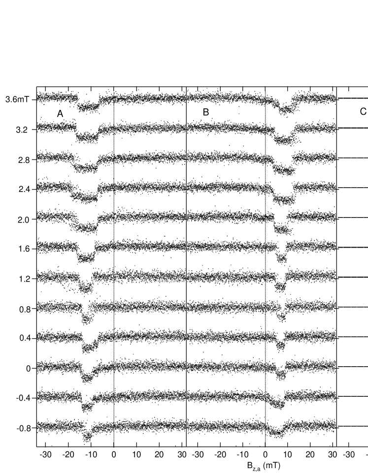
Figure 4: A and B: Spin-valve signals versus weak perpendicular field $B_{x,a}$, for decreasing and increasing $B_{z,a}$, respectively, at $T=4.2K$. C: Calculated spin-valve signal corresponding to Fig. 4-B.

The reason that the spin-valve signal in Fig. 4 is weakly affected by the perpendicular field, compared to the effect at $B_{z,a}=0$ shown in Figs. 3A and B, is that in the spin valve signal, $B_{z,a}$ is large compared to $B_{x,a}$ in the antiparallel magnetic configuration, so the spin-valve signal has reduced sensitivity to the perpendicular field. Fig. 4-C displays the spin-valve signal versus increasing $B_{x,a}$ calculated from Eq. 1 as explained above, showing that the perpendicular field in Fig. 4 is weak to suppress the amplitude of the spin-valve signal. The calculation for decreasing $B_{x,a}$ leads to the same conclusion.

Initially, we studied the effect of the magnetic field applied along the hard axis ($B_{y,a}$) in this sample. The spin valve signal was significantly weakened with a strong hard axis field, analogous to the effect in Figs. 3 D,F, and G. But, in zero applied field, $B_{x,a}=B_{z,a}=0$, we could not resolve any dependence in $I$ versus $B_{y,a}$ beyond noise. The absence of minimum with $B_{y,a}$ is explained by the large component of the local field along the $x$ direction. Using Eq. 1, the amplitude of the minimum in $I$ versus $B_{y,a}$ should be $\Delta I\frac{B_{z,l}^{2}}{B_{z,l}^{2}+B_{x,l}^{2}}\approx 8fA$, which is less than the noise.

Since the dominant component of $\vec{B_{l}}$ is along $x$, this suggests that the local field is generated by a domain magnetized along the x-direction, in the vicinity of the nanoparticle. Such a domain would explain the hysteresis and asymmetry in Figs. 3-A and B, if the domain wall moved in response to changing $B_{x,a}$. In that case the local field would not be completely independent of the applied field. Hysteresis of the domain wall motion would lead to a hysteresis in $B_{x,l}$. The asymmetry of the minimum could also be attributed to the dependence of $B_{x,l}$ on $B_{x,a}$. But the hysteresis in $B_{x,l}$ is only $0.2mT$, which is about 10%. So, in the lowest order of approximation, it can be assumed that the local field is constant in our applied field range.

The spin filter model is valid if the dephasing is weak. In a single metallic nanoparticle, the dephasing is caused by temporal fluctuations of the magnetic field, which can randomize the spin angle with respect to the z-axis. The current through the nanoparticle in contact with ferromagnetic leads in the presence of dephasing was calculated recently by Braun et al. Braun et al. (2005) Their model leads to the formula

$$\Delta I(\alpha)\sim\frac{\omega_{B_{z}}^{2}}{\nu_{S}^{2}+\omega_{B_{z}}^{2}+\omega_{B_{\perp}}^{2}},$$ (2)

where $\vec{\omega}_{B}=g\mu_{B}\vec{B}/\hbar$. This dependence is identical to that in Eq. 1, except for the dephasing term in the denominator. The dephasing term increases the width of the minimum in current versus perpendicular field. The dephasing is negligible if $g\mu_{B}B>\nu_{S}$. Eq. 2 can be used to obtain a lower limit for the spin-dephasing time in the nanoparticle: $T_{2}=1/\nu_{S}>\hbar/g\mu_{B}\sqrt{B_{z,l}^{2}+B_{y,l}^{2}}=8nS$. The dephasing time in the nanoparticle is enhanced compared to that in mesoscopic Al strips, Jedema et al. (2001) and it is more in line with the lower bounds of $T_{2}$ measured in GaAs quantum dots. Petta et al. (2004)

In conclusion, spin polarized current through an Aluminum nanoparticle is very sensitive to the direction of the magnetic field and consistent with a picture in which the nanoparticle states filter spin polarized current by selecting the spinor component specified by the magnetic field. A magnetic field applied perpendicular to the direction of the magnetizations suppresses spin polarized current. A lower bound of the spin dephasing time, 8ns, is obtained from the characteristic field for that suppression. As a function of bias voltage, a stepwise increase in spin polarized current is observed when an additional charged state of the nanoparticle becomes conductive, confirming that spin-relaxation time is $\sim\mu s$ only if the nanoparticle is in the ground state or very close to it.

This research is supported by the DOE grant DE-FG02-06ER46281 and David and Lucile Packard Foundation grant 2000-13874.

References

- Petta et al. (2004) J. R. Petta, A. C. Johnson, J. M. Taylor, E. A. Laird, A. Y. A, M. D. Lukin, C. M. Marcus, M. P. Hanson, and A. C. Gossard, Science 309, 2180 (2004).
- Koppens et al. (2006) F. H. L. Koppens, C. Buizert, K. J. Tielrooij, I. T. Vink, K. C. Nowack, T. Meunier, L. P. Kouwenhoven, and L. M. K. Vandersypen, Nature 442, 766 (2006).
- Jedema et al. (2001) F. J. Jedema, A. T. Filip, and B. J. van Wees, Nature 410, 345 (2001).
- Wei et al. (2008) Y. G. Wei, C. E. Malec, and D. Davidovic, Phys. Rev. B 78, 035435 (2008).
- Salinas et al. (1999) D. G. Salinas, S. Gueron, D. C. Ralph, C. T. Black, and M. Tinkham, Phys. Rev. B 60, 6137 (1999).
- Brouwer et al. (2000) P. W. Brouwer, X. Waintal, and B. I. Halperin, Phys. Rev. Lett. 85, 369 (2000).
- Matveev et al. (2000) K. A. Matveev, L. I. Glazman, and A. I. Larkin, Phys. Rev. Lett. 85, 2789 (2000).
- Bernand-Mantel et al. (2006) A. Bernand-Mantel, P. Seneor, N. Lidgi, M. Munoz, V. Cros, S. Fusil, K. Bouzehouane, C. Deranlot, A. Vaures, F. Petroff, et al., Appl. Phys. Lett. 89, 062502 (2006).
- Wei et al. (2007) Y. G. Wei, C. E. Malec, and D. Davidovic, Phys. Rev. B 76, 195327 (2007).
- Mitani et al. (2008) S. Mitani, Y. Nogi, H. Wang, K. Yakushiji, F. Ernult, and K. T. K, Appl. Phys. Lett. 92, 152509 (2008).
- Deshmukh and Ralph (2002) M. M. Deshmukh and D. C. Ralph, Phys. Rev. Lett 89, 266803 (2002).
- Santos and Moodera (2004) T. S. Santos and J. S. Moodera, Phys. Rev. B 69, 241203(R) (2004).
- Gajek et al. (2005) M. Gajek, M. Bibes, A. Barthelemy, K. Bouzehouane, S. Fusil, M. Varela, J. Fontcuberta, and A. Fert, Phys. Rev. B 72, 020406(R) (2005).
- Ramos et al. (2007) A. V. Ramos, M.-J. Guittet, J. B. Moussy, R. Mattana, C. Deranlot, F. Petroff, and C. Gatel, Appl. Phys. Lett. 91, 122107 (2007).
- Slonczewski (1989) J. C. Slonczewski, Phys. Rev. B 39, 6995 (1989).
- Brataas et al. (1999) A. Brataas, Y. V. Nazarov, J. Inoue, and G. E. W. Bauer, Phys. Rev. B 59, 93 (1999).
- Weymann et al. (20053) I. Weymann, J. Konig, J. Martinek, J. Barnas, and G. Schon, Phys. Rev. B 72, 115334 (20053).
- Braun et al. (2004) M. Braun, J. Konig, and J. Martinek, Phys. Rev. B 70, 195345 (2004).
- Johnson and Silsbee (1985) M. Johnson and R. H. Silsbee, Phys. Rev. Lett. 55, 1790 (1985).
- Averin and Likharev (1991) D. V. Averin and K. K. Likharev, in Mesoscopic Phenomena in Solids, edited by B. L. Altshuler, P. L. Lee, and R. A. Webb (Elsevier and Amsterdam, 1991), p. 169.
- Braun et al. (2005) M. Braun, J. Konig, and J. Martinek, Europhys. Lett. 72, 294 (2005).
- Ralph et al. (1995) D. C. Ralph, C. T. Black, and M. Tinkham, Phys. Rev. Lett. 74, 3241 (1995).