Contact process with long-range interactions: a study in the ensemble of constant particle number

Abstract

We analyze the properties of the contact process with long-range interactions by the use of a kinetic ensemble in which the total number of particles is strictly conserved. In this ensemble, both annihilation and creation processes are replaced by an unique process in which a particle of the system chosen at random leaves its place and jumps to an active site. The present approach is particularly useful for determining the transition point and the nature of the transition, whether continuous or discontinuous, by evaluating the fractal dimension of the cluster at the emergence of the phase transition. We also present another criterion appropriate to identify the phase transition that consists of studying the system in the supercritical regime, where the presence of a “loop” characterizes the first-order transition. All results obtained by the present approach are in full agreement with those obtained by using the constant rate ensemble, supporting that, in the thermodynamic limit the results from distinct ensembles are equivalent.

PACS numbers: 05.70.Ln, 05.50.+q, 05.65.+b

I Introduction

The study of equivalence of ensembles that describe systems in thermodynamic equilibrium, the Gibbs ensembles, has a long tradition in statistical mechanics. Thermodynamic properties evaluated in distinct ensembles will be the same if they are equivalent. In the case of equilibrium systems, the ensembles are set up according to well known prescriptions that take account the existence of a Hamiltonian land58 ; ruel69 . The possibility of representing nonequilibrium systems in distinct ensembles was first considered by Ziff and Brosillow ziff92 when they used the constant coverage ensemble to study first-order transitions in a catalytic reaction model ziff86 , originally defined in the ensemble of constant rate. Afterwards, Tomé and de Oliveira tome01 introduced the conserved contact process, a version of the contact process marr99 ; harr74 in the ensemble of constant particle number. The equivalence between the constant rate and constant particle number ensembles for the contact process in the stationary regime has been proved by Hilhorst and van Wijland in the thermodynamic limit hilh02 . Later on, the equivalence of ensembles in the stationary regime was extended for other systems with short-range interactions with distinct annihilation dynamics oliv03 ; fior05 .

In equilibrium statistical mechanics, the equivalence of ensembles is granted for homogeneous and extensive systems in the thermodynamic limit land58 ; ruel69 ; gross . On the other hand, for non-extensive systems, the canonical and microcanonical ensembles are not equivalent bell68 . Examples of physical problems in which canonical and microcanonical ensembles are not equivalent are nuclei, atomic clusters in which the range of forces between their constituents are comparable to the system size, systems at the first-order transition with phase separation gross ; thirring and models with long-range forces gross ; barr01 ; dauxois . In particular, this latter set of problems has deserved a great interest not only in statistical mechanics, but also in other areas, such as nuclear physics, astrophysics bell68 and plasma physics smith . Nonequilibrium systems with long-range interactions have also been proposed and in this case, we may ask whether the equivalence of ensembles may be valid for such systems.

In the context of nonequilibrium statistical mechanics, systems displaying long-range interactions have been proposed originally as more realistic models describing the spreading processes, instead of short-range systems. In particular, an anomalous model of the directed percolation has been proposed by Mollison mollison . In this problem, the infection probability performs a Lévy flight decaying with the distance $r$ as a power-law relation $1/r^{\sigma+d}$, where $d$ is the spatial dimension of the system and $\sigma$ is control parameter. The critical behavior of anomalous directed percolation displays a family of universality classes that have been studied by Grassberger grass86 , by Janssen et al jan99 who have considered field-theoretic renormalization group, by Hinrichsen and Howard hinri99 who performed numerical simulations and recently by Tessone et al tessone who analyzed a class of spatially extended chaotic systems with power-law decaying interactions. In all cases above, the critical exponents vary continuously with the parameter $\sigma$. More recently, another class of nonequilibrium systems with long-range interactions, named contact processes with long-range interactions, have been introduced by Ginelli et al. gine05 ; gine06 ; hinri07 , inspired by pinning-depinning transitions in nonequilibrium wetting phenomena. By varying the control parameters, the contact process with long-range interactions exhibits a richer phase diagram than the usual short-range contact process, with distinct universality classes gine06 and discontinuous phase transitions gine05 ; gine06 .

Two aims concern us in this paper. First, we wish to analyze the equivalence of ensembles in nonequilibrium systems with long-range interactions. The equivalence of ensembles has been studied in systems with short-range interactions tome01 ; saba02 ; fior05 ; fior04 , but not in systems with long-range interactions. We will consider here the $\sigma-$contact process with long-range interactions, introduced by Ginelli et al gine05 . Second, we wish to show that the present approach offers a new procedure for analyzing first-order transitions of systems with absorbing states. Due to the existence of the absorbing states, standard procedures used successfully in the study of discontinuous equilibrium phase transitions may not work well when applied to describe nonequilibrium first-order transitions. In the present case, the first evidence for a discontinuous transition will be given by the presence of “loops” in the rate versus density curve, as long as the system is finite. As it will be shown, the loops disappear in the thermodynamic limit giving rise to a tie line, the true signature of a first-order transition. Another advantage of using the present approach is verified when one analyzes the system at the emergence of the phase transition, since the nature of the phase transition can be inferred simply by examinating the structure of particles. As we shall see, if, at the emergence of the transition, the cluster is fractal, the transition will be continuous; if the cluster is compact, the transition will be discontinuous. A compact cluster provides us an evidence of a discontinuous transition.

II Model

II.1 Constant rate ensemble

The one dimensional $\sigma-$contact process with long-range interactions gine05 is defined in a chain of $L$ sites with periodic boundary conditions as follows. To each site $i$ of a one-dimensional lattice is attached an occupation variable $\eta_{i}$ that takes the values 0 or 1 according whether the site $i$ is empty or occupied by a particle, respectively. The process is composed of spontaneous annihilation of a single particle ($1\to 0$) and catalytic creation of a particle ($0\to 1$). Particles are created only in empty sites in which at least one of its nearest neighbor sites is occupied by a particle. These empty sites are named active sites. The rate of creation depends on the length of the island of empty sites next to the active site and decreases algebraically with the size of the island, introducing an effective long-range interaction. The total transition rate $w_{i}(\eta)$ is given by

$$w_{i}(\eta)=\omega_{i}^{c}(\eta)+\alpha\omega_{i}^{a}(\eta),$$ (1)

where $\alpha$ is a parameter and

$$\omega_{i}^{a}(\eta)=\eta_{i},$$ (2)

describes a spontaneous annihilation and

$$\omega_{i}^{c}(\eta)=\frac{1}{2}\,\sum_{\ell=1}^{\infty}(1+\frac{a}{\ell^{\sigma}})\eta_{i-1}{\bar{\eta}}_{i}{\bar{\eta}}_{i+1}\ldots{\bar{\eta}}_{i+\ell-1}\eta_{i+\ell}$$

$$+\frac{1}{2}\,\sum_{\ell=1}^{\infty}(1+\frac{a}{\ell^{\sigma}})\eta_{i+1}{\bar{\eta}}_{i}{\bar{\eta}}_{i-1}\ldots{\bar{\eta}}_{i-\ell+1}\eta_{i-\ell},$$ (3)

describes a catalytic creation that depends on the length $\ell$ of the island of empty sites, where $a$ and $\sigma$ are parameters and we have considered the shorthand notation ${\bar{\eta}}_{i}\equiv 1-\eta_{i}$ in Eq. (3). When $a=0$ one recovers the original short-range contact process marr99 ; harr74 .

Here, numerical simulations in the constant rate ensemble is performed as follows. A particle is chosen at random from a list of occupied sites. It is annihilated with probability $p=\alpha/(1+a+\alpha)$. With probability $1-p$, a new particle may be created next to the chosen particle. This is done by choosing first one of its two nearest neighbors with equal probability and then a particle will be actually created with probability $q=(1+a\ell^{-\sigma})/(1+a)$ provided the chosen site is empty. This algorithm gives the following ratio between the creation and annihilation of particles $(1-p)q/2p=(1+a\ell^{-\sigma})/2\alpha$, which is equivalent to that considered by Ginelli et al gine05 , in which the creation and annihilation of particles occur with rates $\lambda(1+a\ell^{-\sigma})$ and $1$, respectively as long as $\alpha$ is related to $\lambda$ by $\alpha=1/2\lambda$. The increment of the time is given by $1/N_{p}$, where $N_{p}$ is the number of occupied sites.

For large values of $\alpha$, the system is constrained into the absorbing state, in which no particles are allowed to be created. Decreasing the parameter $\alpha$, a phase transition to an active state takes place, whose location depends on the parameters $a$ and $\sigma$. For a fixed value of $a$ (we take here to be $a=2$, as considered by Ginelli et al. gine05 ) and $\sigma>1$ the transition is continuous with critical exponents belonging to direct percolation (DP) universality class. For $0<\sigma<1$ the transition becomes discontinuous. Ginelli et al gine05 found that, the crossover between the discontinuous and second-order phase transitions occurs at $\sigma=1.0$.

II.2 Constant particle number ensemble

In the constant particle number ensemble, the control parameter is the total particle number $n$. Again we used a chain with $L$ sites with periodic boundary conditions. Particles are neither created nor annihilated. Instead, a particle leaves their place and jump to an empty site. However, the jump process is not unrestrictive process, since their occurrence must be consistent with the rules of their version in the constant rate ensemble. More specifically, the dynamics that characterizes this ensemble is defined as follows. A particle of the system, chosen at random, leaves its place, located for example at the site $i$, and jumps to an empty site placed at the site $j$, also chosen at random. The jump rate will depend on the specific rule of the considered model. One may define the jump process by a dynamics in which both creation and annihilation occurs simultaneously, according to the transition rate $w_{ij}(\eta)$ is given by tome01 ; oliv03 ; fior05

$$w_{ij}(\eta)=\omega_{i}^{a}(\eta)\omega_{j}^{c}(\eta).$$ (4)

To see that this transition rate leads to a dynamic that is equivalent to that given by Eq. (1) let us consider the total rate $\sum_{i}w_{ij}(\eta)/L=\sum_{i}\omega_{i}^{a}(\eta)\omega_{j}^{c}(\eta)/L$ in which particles jump to site $j$. In the thermodynamic limit the system size $L\rightarrow\infty$ and the sum $\sum_{i}\omega_{i}^{a}(\eta)/L$ approaches $\langle\omega_{i}^{a}(\eta)\rangle$, by the law of large numbers, so that $\sum_{i}w_{ij}(\eta)/L=\langle\omega_{i}^{a}(\eta)\rangle\omega_{j}^{c}(\eta)$. By an analogous argument the total rate in which particles leave the site $i$ is $\sum_{j}w_{ij}(\eta)/L=\langle\omega_{j}^{c}(\eta)\rangle\omega_{i}^{a}(\eta)$. Comparing with the Eq. (1), the averages $\langle\omega_{i}^{a}(\eta)\rangle$ and $\langle\omega_{i}^{c}(\eta)\rangle$ should be proportional to $1$ and $\alpha$, respectively, thus

$${\bar{\alpha}}=\frac{\langle\omega_{j}^{c}(\eta)\rangle}{\langle\omega_{i}^{a}(\eta)\rangle},$$ (5)

where $\omega_{j}^{c}(\eta)$ and $\omega_{i}^{a}(\eta)$ are given by Eqs. (2) and (3), respectively, so that Eq. (6) is given by

$${\bar{\alpha}}=\frac{1}{\rho}\langle\omega_{j}^{c}(\eta)\rangle,$$ (6)

where $\langle\omega_{i}^{a}(\eta)\rangle=\langle\eta_{i}\rangle=\rho$ is the density of particles. This formula allow us to evaluate the parameter ${\bar{\alpha}}$ within respect to the ensemble of constant particle number. The average $\langle\omega_{j}^{c}(\eta)\rangle$ can be understood as “density of active sites”, that is, the density of empty sites in which particles may jump to them. It can be evaluated directly from numerical simulations by computing Eq. (3) that is zero and $(1+a\ell^{-\sigma})/2$ according whether the site $i$ is occupied or empty, respectively, where $\ell$ is the length of the island of inactive sites in which the active site is located. For time-dependent regime, however, Eq. (6) might not always hold. For instance, if the initial state is such that averages $\langle\omega_{j}^{c}(\eta)\rangle$ and $\langle\omega_{i}^{a}(\eta)\rangle$ are not constants, Eq. (6) cannot be satisfied hilh02 ; oliv03 .

The actual numerical simulation of the constant particle number ensemble is realized as follows. An empty site surrounded by at least one particle (active site) is chosen at random. Next, a particle of the system, also chosen at random, jumps to the active site with probability $p_{\ell}=(1+a\ell^{-\sigma})/(1+a)$. The constant factor $1/(1+a)$ is used in order to guarantee that $p_{\ell}\leq 1$, since $1+a\ell^{-\sigma}$ may be greater than $1$. In the constant rate ensemble, the control parameter may be included in the probability of choosing each subprocess (creation or annihilation). However, in the present case, as both processes occur simultaneously and the parameter $\bar{\alpha}$ is not constant, this procedure is not possible.

In contrast to the constant rate ensemble, the conserved contact process does not have, strictly speaking, an absorbing state. This fact constitutes an useful tool in the study of phase transitions because there is no danger of falling into the absorbing state as happens in numerical simulations of the constant rate ensemble. In the conserved ensemble (constant particle number ensemble) the equivalent of the absorbing state is the state with zero density, as is the case of an infinite system with a finite number of particles, also named subcritical regime.

III Cluster approximations

The first analysis we have performed here consists of studying the $\sigma-$contact process by means of cluster approximations. We will consider here approximations at the level of one and two sites.

At the level of one-site approximation, we use the following approximation for the probability of a string of sites:

$$P(\eta_{1},\eta_{2},...,\eta_{\ell})=P(\eta_{1})P(\eta_{2})...P(\eta_{\ell}).$$ (7)

In this case, it suffices to consider the dynamic variables $P(1)=\rho$ and $P(0)=1-\rho$. In the steady state, one has the following relation

$$\alpha=1-\rho+a\rho\sum_{\ell=1}^{\infty}\frac{(1-\rho)^{\ell}}{\ell^{\sigma}}.$$ (8)

This equation has already been obtained by Ginelli et al gine05 ; hinri07 . For $0<\sigma<1$, Eq. (8) establishes a discontinuous transition between an absorbing and an active state that can be viewed by the existence of “loops” loops . As it will be seen later, numerical simulations in the constant particle number ensemble also presents “loops” for finite systems in the interval $0<\sigma<1$. However, Eq. (8) also exhibits loops for $\sigma>1$, in contrast to numerical simulations.

In order to obtain improved results, we have derived relations by considering correlations of two sites. In this case, the probability of a string of sites is approximated by

$$P(\eta_{1},\eta_{2},\eta_{3},...,\eta_{\ell})=\frac{P(\eta_{1},\eta_{2})P(\eta_{2},\eta_{3})...P(\eta_{\ell-1},\eta_{\ell})}{P(\eta_{2})P(\eta_{3})...P(\eta_{\ell-1})}.$$ (9)

The dynamic variables are now $P(1),P(0)$ and nearest-neighbor joint probabilities $P(11),P(10)=P(01)$ and $P(00)$. Only two of them are independent, so that it is necessary to write down two equations. By solving these equations numerically, we find the behavior of $\alpha$ versus $\rho$ for several values of $\sigma$, as showed in Fig 1.

Figure 1: Quantity $\alpha$ versus $\rho$ for several values of $\sigma$ at the level of two-site mean field approximation. A crossover from a first-order to a continuous transitions occurs at $\sigma=(1.3\pm 0.1)$. Symbols have been used in order to distinguish the distinct values of $\sigma$.

In contrast to the previous case, two-site approximations supports a change in the nature of the phase transition by increasing the parameter $\sigma$, passing from first-order to second-order at $\sigma=(1.3\pm 0.1)$. This can be identified by disappearance of loops. Although the results obtained from two-site approximations agree qualitatively with numerical simulations, the location of the transition points as well as the value of $\sigma$ that characterizes the crossover between first-order and second-order transitions are incorrect.

IV Numerical results

Numerical simulations of the $\sigma-$contact process were performed for $a=2$ and several values of $\sigma$. We have used $2\times 10^{7}$ Monte Carlo steps to evaluate the appropriate quantities, after discarding a sufficient number of steps to reach the stationary state. Here one Monte Carlo step corresponds to $n$ jumping processes. In order to compare results obtained from distinct ensembles we have simulated the contact process with long-range interactions not only in the constant particle number ensemble, but also in the constant rate ensemble. We have first determined the quantity ${\bar{\alpha}}$ in the conserved (constant particle number) ensemble, by using Eq. (1), for several densities $\rho$. Next we used the values of ${\bar{\alpha}}=\alpha$ to perform numerical simulations in the constant rate ensemble which in turn gives us the average density ${\bar{\rho}}$. According to Table I, the excellent agreement between the results confirms the equivalence of ensembles. However, numerical simulations provide distinct results at the phase coexistence, even when one considers large system sizes. For example, for $L=20000$ and $\sigma=0.5$, simulations in the constant rate ensemble for $\alpha=0.42313$ gives $\bar{\rho}=0.76600(4)$. This value of $\alpha$ corresponds to two densities in the constant particle number ensemble $\rho=0.60$ and $\rho=0.766$. As it will be shown later, both ensembles become equivalent at the phase coexistence in the thermodynamic limit.

From now on we will drop the bars over ${\bar{\alpha}}$ and ${\bar{\rho}}$.

Table 1: Results of numerical simulations coming from the constant particle number ensemble (second and third columns) and from the constant rate ensemble (fourth and fifth columns) for a system size $L=20000$.

$\sigma$	$\rho$	${\bar{\alpha}}$	$\alpha$	${\bar{\rho}}$
2.0	0.7500	0.2964(4)	0.29638	0.7509(9)
1.5	0.6900	0.33481(1)	0.33480	0.6900(1)
1.0	0.7000	0.37007(1)	0.37000	0.7004(2)
0.5	0.8500	0.32887(8)	0.32890	0.85008(8)
0.4	0.9000	0.24948(2)	0.24948	0.90000(1)

IV.1 Subcritical regime

Figure 2: Quantity $\alpha$ versus $1/n$ for the subcritical regime. The left, center and right panels correspond to $\sigma=2$, $\sigma=0.5$ and $\sigma=0.4$, respectively. The straight lines fitted to the data points give the extrapolated critical points $\alpha_{0}=0.35497$, $\alpha_{0}=0.41389$ and $\alpha_{0}=0.41714$.

Let us consider a finite number of particles placed on infinite lattice. In this situation the density of particles vanishes and the system is constrained to remain in the subcritical regime. The actual simulation of the subcritical regime is done by using a finite lattice and check whether a particle reaches the border. If a particle never reaches the border, the system size may be taken as infinite. The size of the system was chosen to be big enough, so that no particles have reached the border for the maximum time considered. An important feature of the subcritical regime is that the increase of the total number of particles makes the system approach the transition point at $\alpha=\alpha_{0}$. The expected value of $\alpha$ obtained for a fixed number of particles $n$ approaches its asymptotic value $\alpha_{0}$ according to tome01 ; saba02 ; fior05 ; fior04

$$\alpha-\alpha_{0}\sim\frac{1}{n}.$$ (10)

A linear extrapolation of $\alpha$ versus $1/n$ when $n\to\infty$ gives $\alpha_{0}$. In Fig. 2 we have plotted the numerical values of $\alpha$ determined from simulations of an infinite system with $n$ particles for different values of $\sigma$. Numerical extrapolations obtained by using Eq. (10) give us $\alpha_{0}=0.41714(6)$, $\alpha_{0}=0.41389(1)$ and $\alpha_{0}=0.35497(6)$ for $\sigma=0.4$, $\sigma=0.5$ and $\sigma=2$, respectively, which agree very well with estimates $\alpha_{0}=0.4172(1)$, $\alpha_{0}=0.41382(3)$ and $\alpha_{0}=0.3548(2)$, obtained from the constant rate ensemble. The same agreement is verified for other values of $\sigma$, revealing the utility of the present procedure for locating the transition point. In the section IV C, we will show results from time-dependent numerical simulations for $\sigma=0.4$. For $a=0$, the phase transition takes place at $\alpha_{0}=0.303228(2)$, as expected for the usual short-range contact process marr99 .

Figure 3: Typical run for the conserved long-range contact process with $n=50$ particles for $\sigma=2$ starting from a random configuration. A unit of time, or a Monte Carlo step, corresponds to $n$ particle jumps. We have discarded $3\times 10^{6}$ initial Monte Carlo steps.

Figure 4: Typical run for the conserved long-range contact process with $n=50$ particles for $\sigma=0.5$ starting from a random configuration. A unit of time, or a Monte Carlo step, corresponds to $n$ particle jumps. We have discarded $3\times 10^{6}$ initial Monte Carlo steps.

The first procedure considered here for classifying the phase transition consists of examinating the spatial structure of particles at the emergence of the phase transition. In Figs. 3 and 4 we have plotted the time evolution for two distinct values of $\sigma$. For $\sigma=2$, the system generates fractal clusters, whereas for $\sigma=0.5$ they are compact.

A measure of the size of the cluster of particles is given by the quantity $R$ given by maximum distance between two particles of the cluster saba02 ; brok99 . As long as $n$ is finite, $R$ is also finite, but it diverges when $n\rightarrow\infty$. It is related to the total particle number $n$ through the relation

$$R\sim n^{1/d_{F}},$$ (11)

where $d_{F}$ is the fractal dimension saba02 ; brok99 . The quantity $R$ will be evaluated here by measuring the end-to-end spread of the cluster saba02 ; fior05 ; fior04 ; brok99 .

Figure 5: Log-log plot of the average cluster size $R$ versus the total number of particles $n$ for several values of $\sigma$ at the subcritical regime. The straight lines from top to bottom have slopes 1.33704 and 1, respectively. The data points have been shifted in order to avoid overlapping.

In Fig. 4 we show the log-log plot of $R$ versus $n$ in the subcritical regime for several values of $\sigma$. For $\sigma>1$, the slopes of the straight lines fitted to the data points are consistent with $1.33704(4)$, as expected for the DP universality class whose clusters generated at the criticality vics92 have fractal dimension $d_{F}=0.74792(2)$ marr99 , whereas for $0<\sigma<1$ the slopes are equal to $1$. The change in the fractal dimension shows the change in the nature of the phase transition, passing from continuous to discontinuous, as one decreases $\sigma$. A fractal dimension equal to the Euclidean dimension is actually the signature of a first order transition, since we have a compact cluster that remains finite in the thermodynamic limit. To see this, let us evaluate the density $\rho^{*}$ of the cluster of particles $\rho^{*}=n/R$. It is worth emphasizing that although the total density $\rho=n/L$ of the system is zero, since the system is constrained in the subcritical regime, the quantity $\rho^{*}$ is finite. If the phase transition is first order, $\rho^{*}$ will have a non-zero value in the thermodynamic limit. Rewriting Eq. (11) in terms of $\rho^{*}$, one has the following relation $\rho^{*}=n/R\sim n^{-(1-d_{F})/d_{F}}$. Therefore, for $0<\sigma<1$, where $d_{F}=1$, $\rho^{*}\rightarrow\rho^{*}_{0}$, when $n\rightarrow\infty$, corresponding to the active phase $\rho^{*}_{0}$ in coexistence with the absorbing phase ($\rho=0$). The density $\rho^{*}_{0}$ is determined simply by the inverse of the slope of curves in Eq. (11). In contrast, for a second order transition in which $d_{F}<1$, $\rho^{*}$ vanishes when $n\to\infty$, because $\rho^{*}=n/R\sim n^{-(1-d_{F})/d_{F}}\rightarrow 0$ when $n\rightarrow\infty$. The change in the nature of the phase transition for $\sigma$ close to 1 is in agreement with results by Ginelli et al gine05 who used time-dependent numerical simulations and distribution of inactive islands to identify the order of the phase transition.

We close this section by comparing the density $\rho^{*}_{0}$ of the compact cluster obtained from both ensembles. As it was mentioned above, in the constant particle number ensemble the density $\rho^{*}_{0}$ is evaluated directly, since it is simply the inverse of the slope of Eq. (11). To determine $\rho^{*}_{0}$ in the constant rate ensemble, we use the procedure adopted by Dickman dick91 ; maia07 that consists of dividing the system into blocks of 100 sites and determining histograms of such blocks density profiles at the phase coexistence. For $\sigma=0.5$ at the phase coexistence, the histogram show a bimodal distribution with a peak at $\rho^{*}=0$ and another one at $\rho^{*}_{0}=0.77$. This agrees with the density of the compact cluster $\rho^{*}_{0}=0.777(1)$, obtained from the present approach (constant particle number ensemble). For other values of $\sigma$ in the interval $0<\sigma<1$, the densities of compact clusters at the phase coexistence obtained from both ensembles agree very well.

IV.2 Supercritical regime

Figure 6: Quantity $\alpha$ versus $\rho$ for several values of the system size $L$ for $\sigma=2$. The inset shows the collapse of the data by using relation (12) and (13) where $y=L^{1/\nu_{\perp}}|\alpha-\alpha_{0}|$ and $x=L^{\beta/\nu_{\perp}}\rho$ for the supercritical regime and $y=L^{d_{F}}|\alpha-\alpha_{0}|$ and $x=L^{d-d_{F}}\rho$ for the subcritical regime.

Figure 7: Quantity $\alpha$ versus $\rho$ for several values of the system size $L$ for $\sigma=0.5$. The horizontal straight line is the tie line at $\alpha=\alpha_{0}=0.41389$. The dashed vertical line indicates the density $\rho^{*}=0.777$ of the coexisting active phase. The inset shows the collapse of the data by using relation (14) $y=(\alpha-\alpha_{0})L^{\sigma}$.

The supercritical regime is characterized by nonzero values of the density $\rho$. To simulate the $\sigma-$contact process in the supercritical regime, we have considered lattice sizes ranging from $L=200$ to $L=20000$. In Figs. 6 and 7 we have plotted the quantity $\alpha$ versus $\rho$ for several values of $L$ for $\sigma=2$ and $\sigma=0.5$, respectively. The curves exhibit a strong dependence on $L$ that is qualitatively different whether we consider $\sigma>1$ or $0<\sigma<1$. In the first case (exemplified in Fig. 6 by $\sigma=2$), the curves are strictly decreasing functions and cumulated, when $L\to\infty$, into a strictly decreasing function.

In the second case (exemplified in Fig. 7 by $\sigma=0.5$), the curves are no longer decreasing and present “loops”, that can be associated to a coexistence of two phases. As it was shown previously, the occurrence of “loops” in numerical simulations agrees qualitatively mean-field results. However, in contrast to the mean-field approach, the existence of “loops” in numerical simulations is a finite size effect that disappears when $L\rightarrow\infty$, giving rise to a horizontal tie line that connects the two coexisting phases.

For $\sigma>1$, where the phase transition is second order, the finite size scaling for the density is given by tome01

$$\rho=L^{-\beta/\nu_{\perp}}f(\epsilon L^{1/\nu_{\perp}}),$$ (12)

valid for the supercritical regime, where $\epsilon=\alpha-\alpha_{0}$ and $\beta$ and $\nu_{\perp}$ are critical exponents associated to the order parameter and the spatial correlation length, respectively; and tome01

$$\rho=L^{-d+d_{F}}f(\epsilon L^{d_{F}}),$$ (13)

valid in the subcritical regime, where $f(x)$ is an universal function. A data collapse obtained by using the finite size scalings (12) and (13) and the best estimates of the DP critical exponents $\beta=0.276486(8)$, $\nu_{\perp}=1.096854(4)$ and $d_{F}=0.74792(2)$ marr99 is shown in the inset of Fig. 6.

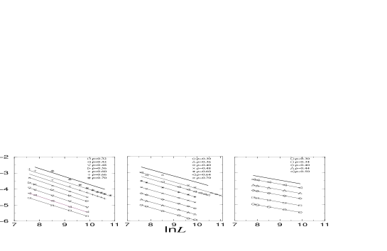
Figure 8: Log-log plot of $\alpha-\alpha_{0}$ versus $L$ for several densities $\rho$ for $\sigma=0.5$ (left panel), $\sigma=0.4$ (center panel) and $\sigma=0.25$ (right panel). From left to right, the straight lines at each panel have slopes $0.5$, $0.4$ and $0.25$. The data points have been shifted in order to avoid overlapping.

On the other hand, for $0<\sigma<1$, where the phase transition is first order, Eqs. (12) and (13) are not valid. To relate the parameter $\alpha$ with the system size $L$, we assume the following behavior of $\alpha$ in the region of the phase coexistence

$$\alpha-\alpha_{0}\sim L^{-\sigma},$$ (14)

where $\alpha_{0}$ is the value of $\alpha$ at the coexistence, or the value of $\alpha$ where the tie line is located.

An argumentation concerning Eq. (14) is given by assuming the one-site mean-field approximation given by Eq. (8). For $0<\sigma<1$, the sum on the right side of Eq. (8) can be replaced by an integral, which to leading order in $\rho$, reduces to gine05 ; gine06

$$\alpha-\bar{\alpha_{0}}=-\rho+a\Gamma(1-\sigma)\rho^{\sigma}.$$ (15)

where $\bar{\alpha_{0}}=1$ is its one-site mean-field transition value and $\Gamma(x)$ is the gamma function. Relating $\rho$ with the system size $L$, we have that $\alpha-\bar{\alpha_{0}}\sim L^{-\sigma}$, because the second term in the right-hand side of Eq. (15) dominates over the first.

The correctness of Eq. (14) can be checked by the log-log plot of $\alpha-\alpha_{0}$ versus $L$ by using the estimation of $\alpha_{0}$ available from the study of the subcritical regime. Indeed, as shown in Fig. 8 the slopes of the straight lines fitted to the data points for several densities are consistent with the values of $\sigma$. We have repeated the analysis for other values of $\sigma$ in the interval $0<\sigma<1$, whose dependence of $\alpha$ on the system size $L$ at the phase coexistence is also described by Eq. (14). For higher densities close to $\rho^{*}$, in which one observes a peak of $\alpha$ versus $\rho$, it is necessary to consider larger system sizes in order to reach the asymptotic behavior described by Eq. (14), as can be seen for the highest densities in the left and center panels of Fig. 8, respectively.

A complementar analysis, but fully equivalent, consists in assuming Eq. (14) and using it for determining estimates of $\alpha_{0}$ by numerical extrapolation, as shown in Fig. 9.

Figure 9: Dependence of the parameter $\alpha$ on $L^{-\sigma}$ for $\sigma=0.5$ (left) and $\sigma=0.4$ (right) considering several densities $\rho$. The full circles are extrapolated values of $\alpha_{0}$ obtained from the subcritical regime.

The agreement between extrapolated $\alpha_{0}$ using Eq. (14) and those estimates of $\alpha_{0}$ available from the subcritical regime and spreading simulations (reported in the next section) confirms the equivalence of ensembles in the thermodynamic limit at the phase coexistence.

As a final checking, we plot in the inset of Fig. 7 a collapse of the data for different system sizes by considering the variable $y=(\alpha-\alpha_{0})L^{\sigma}$ versus $\rho$. This confirms once more the conjecture given by Eq. (14).

IV.3 Time dependent numerical simulations

Here, we show explicitly results from time-dependent numerical simulations for the $\sigma-$contact process considering $\sigma=0.4$, in order to compare the results for the estimation of $\alpha_{0}$ from distinct ensembles.

Starting from a configuration close to the absorbing state, this procedure consists in determining the time evolution of appropriate quantities, such as the survival probability $P_{s}(t)$, the total number of particles $N_{p}(t)$ and the mean square spreading $R^{2}(t)$ of the active region. At the emergence of a second-order transition, these quantities are described by following power-law behaviors

$$P_{s}(t)\sim t^{-\delta},\quad N_{p}(t)\sim t^{\eta}\quad{\rm and}\quad R^{2}(t)\sim t^{z},$$ (16)

where $\delta,\eta$ and $z$ are their associated critical exponents. They are related to the fractal dimension introduced in Eq. (11) through the relation $d_{F}=2(\eta+\delta)/z$.

Although the order parameter presents a jump in a nonequilibrium first-order transition, some dynamic variables are also characterized by dynamic exponents odor04 . In the present case, the quantities from Eq. (16) are expected to be described by the same exponents as the Glauber-Ising model at zero temperature, which values are $\delta=1/2$, $\eta=0$ and $z=1$ gine05 . Relating these exponents, we have that $d_{F}=1$, in agreement with results obtained previously from analysis in the subcritical regime for $0<\sigma<1$.

In Fig. (10), we show the plot of temporal evolution of the quantities $P_{s}$, $N_{p}$ for some values of $\alpha$. For $\alpha=0.4172$, the quantities $N_{p}(t)$ and $P_{s}(t)$ follow indeed a power-law behavior described by Eq. (16), whose exponents are consistent to $\eta=0$ and $\delta=1/2$, respectively. This estimation of $\alpha_{0}$ agrees very well to those obtained from the constant particle number ensemble, confirming the equivalence of ensembles.

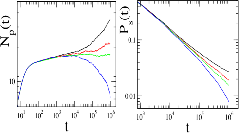
Figure 10: Temporal evolution of the total number of particles $N_{p}$ (right) and the survival probability $P_{s}$ (left) for the ordinary $\sigma-$contact process for $\sigma=0.4$. From top to bottom, we have $\alpha=0.4167$, $0.4171$, $0.4172$ and $0.4176$.

V Conclusion

In this paper we have studied a nonequilibrium model with long-range interactions, named $\sigma-$contact process, in the ensemble of constant particle number. The equivalence of ensembles is confirmed by the excellent agreement between the numerical results coming from both ensembles. All results obtained by the present approach are in full agreement with those obtained by Ginelli et al gine05 . We believe that the present approach may be particularly useful for studying discontinuous phase transition, since it is possible to identify the nature of the transition by measuring the spatial structure of particles at the transition. The interesting feature of the present approach concerns the study of an infinite system with a finite number of particles. As the number of particles is increased, the systems naturally approaches the critical point and, in this sense, it behaves like self-organized critical systems.

Another advantage of the present approach is verified when one studies the system in the supercritical regime. The dependence on the system size is distinct in both regimes as shown in Figs. 6 and 7. The presence of a “loop” is a strong indication of a first-order transition. Of course, results coming from finite systems, such as the “loop” presented in Fig. 7 is a particularity of the conserved ensemble, that disappears in the thermodynamic limit.

We remark that the use of this procedure in the constant rate ensemble is not possible since numerical simulations of finite systems will present a jump in the order parameter close to the transition point, even in the case of a second-order transition, due to the presence of the absorbing state. Recently, de Oliveira and Dickman dic05 have proposed a method, named quasi-stationary simulations, that improves the accuracy of results, even at the emergence of the phase transition. It consists in simulating the system in the constant rate ensemble in the standard way. However, whenever the system enters in the absorbing state, a non-absorbing configuration is chosen from a list of saved periodically configurations and then system returns to the active state. This method has revealed an useful tool in the study of systems with absorbing states gine06 ; maia07 ; dic06 . Other techniques, such as hysteretic analysis in a constant coverage ensemble have also been used to study discontinuous transition in nonequilibrium systems ziff86 ; losc02 ; mone01 . These approaches are, however, distinct from ours, in the sense that the standard ensemble is initially used to generate a stationary configuration and then the system is switched to the constant coverage ensemble.

References

- (1) L. D. Landau and E. M. Lifshitz, Statistical Mechanics (Pergamon Press, Oxford, 1958).
- (2) D. Ruelle, Statistical Mechanics: Rigorous Results (Benjamin, Reading, MA, 1969).
- (3) R. M. Ziff and B. J. Brosilow, Phys. Rev. A 46, 4630 (1992).
- (4) R. M. Ziff, E. Gulari and Y. Barshad, Phys. Rev. Lett. 56, 2553 (1986).
- (5) T. Tomé and M. J. de Oliveira, Phys. Rev. Lett. 86, 5643 (2001).
- (6) J. Marro and R.Dickman, Nonequilibrium Phase Transitions in Lattice Models (Cambridge University Press, Cambridge, England, 1999).
- (7) T. E. Harris, Ann. Probab. 2, 969 (1974).
- (8) H. J. Hilhorst and F. van Wijland, Phys. Rev. E 65, 035103(R) (2002).
- (9) M. J. de Oliveira, Phys. Rev. E 67, 027104 (2003).
- (10) C. E. Fiore and M. J. de Oliveira, Phys. Rev. E 72, 046137 (2005).
- (11) D. H. E. Gross, Microcanical Thermodynamics (world scientific Lecture Notes in Physics, 2001) vol. 66.
- (12) D. Lynden-Bell and R. Wood, Mon. Not. R. Astron. Soc. 138, 495 (1968); D. Lynden-Bell, Physica A 263, 293 (1999).
- (13) W. Thirring, Z. Phys. 235, 339 (1970); P. Hertel and W. Thirring, Ann. of Phys. 63, 520 (1971).
- (14) Some examples of systems in which the ensembles are not equivalent can be found in Refs. J. Barré, D. Mukamel and S. Ruffo, Phys. Rev. Lett. 87, 030601 (2001); A. Campa, S. Ruffo and H. Touchette, cond-mat/0702004.
- (15) T. Dauxois, S. Ruffo, E. Arimondo and M. Wilkens, Dynamics and Thermodynamics of systems with long range interactions, edited by T. Dauxois, S. Ruffo, E. Arimondo and M. Wilkens, Lecture notes in Physics Vol 602 (Springer, Berlin, 2002).
- (16) R. A. Smith and T. M. O’Neil, Phys. Fluids B 2, 2961 (1990).
- (17) D. Mollison, J. R. Stat. Soc. B 39, 283 (1977).
- (18) P. Grassberger, in Fractals in Physics, edited by L. Pietronero and E. Tosatti, (Elsevier, New York, 1986).
- (19) H. K. Janssen, K. Oerding, F. van Wijland and H. J. Hilhorst, Eur. Phys. J. B 7, 137 (1999).
- (20) H. Hinrichsen and M. Howard, Eur. J. Phys. B 7 635 (1999).
- (21) C. J. Tessone, M. Cencini and A. Torcini, Phys. Rev. Lett. 97, 224101 (2006).
- (22) F.Ginelli, H. Hinrichsen, R. Livi, D. Mukamel and A. Politi, Phys. Rev. E 71, 026121 (2005).
- (23) F.Ginelli, H. Hinrichsen, R. Livi, D. Mukamel and A. Torcini, J. Stat. Mech. P08008 (2006).
- (24) H. Hinrichsen, J. Stat. Mech. P07066 (2007).
- (25) M. M. S. Sabag and M. J. de Oliveira, Phys. Rev. E 66, 036115 (2002).
- (26) C. E. Fiore and M. J. de Oliveira, Phys. Rev. E 70, 046131 (2004).
- (27) Loop is an expression borrowed from equilibrium statistical mechanics to design an region of instability, in analogy with the van-der-Waals loops. In this case, the stability conditions are obtained by performing the Maxwell construction.
- (28) H.-M. Bröker and P. Grassberger, Physica A 267, 453 (1999).
- (29) T. Vicsek, Fractal Growth Phenomena, 2nd ed. (World Scientific, Singapoure, 1992).
- (30) R. Dickman and T. Tomé, Phys. Rev. A 44, 4833 (1991).
- (31) D. S. Maia and R. Dickman, J. Phys.: Cond. Matt. 19, 065143 (2007).
- (32) G. Odor, Rev. Mod. Phys, 76, 663 (2004).
- (33) M. M. de Oliveira and R. Dickman, Phys. Rev. E, 71, 016129 (2005).
- (34) M. M. de Oliveira and R. Dickman, Phys. Rev. E, 74, 011124 (2006).
- (35) E. S. Loscar and E. V. Albano Phys. Rev. E 65, 066101 (2002).
- (36) R. A. Monetti and E. V. Albano, J. Phys. A 34, 1103 (2001).