Shell-model calculations and realistic effective interactions

Abstract

A review is presented of the development and current status of nuclear shell-model calculations in which the two-body effective interaction between the valence nucleons is derived from the free nucleon-nucleon potential. The significant progress made in this field within the last decade is emphasized, in particular as regards the so-called $V_{\rm low-k}$ approach to the renormalization of the bare nucleon-nucleon interaction. In the last part of the review we first give a survey of realistic shell-model calculations from early to present days. Then, we report recent results for neutron-rich nuclei near doubly magic ¹³²Sn and for the whole even-mass $N=82$ isotonic chain. These illustrate how shell-model effective interactions derived from modern nucleon-nucleon potentials are able to provide an accurate description of nuclear structure properties.

1 Introduction

The shell model is the basic framework for nuclear structure calculations in terms of nucleons. This model, which entered into nuclear physics more than fifty years ago [1, 2], is based on the assumption that, as a first approximation, each nucleon inside the nucleus moves independently from the others in a spherically symmetric potential including a strong spin-orbit term. Within this approximation the nucleus is considered as an inert core, made up by shells filled up with neutrons and protons paired to angular momentum $J=0$, plus a certain number of external nucleons, the “valence” nucleons. As is well known, this extreme single-particle shell model, supplemented by empirical coupling rules, proved very soon to be able to account for various nuclear properties [3], like the angular momentum and parity of the ground-states of odd-mass nuclei. It was clear from the beginning [4], however, that for a description of nuclei with two or more valence nucleons the “residual” two-body interaction between the valence nucleons had to be taken explicitly into account, the term residual meaning that part of the interaction which is not absorbed into the central potential. This removes the degeneracy of the states belonging to the same configuration and produces a mixing of different configurations. A fascinating account of the early stages of the nuclear shell model is given in the comprehensive review by Talmi [5].

In any shell-model calculation one has to start by defining a “model space”, namely by specifying a set of active single-particle (SP) orbits. It is in this truncated Hilbert space that the Hamiltonian matrix has to be set up and diagonalized. A basic input, as mentioned above, is the residual interaction between valence nucleons. This is in reality a “model-space effective interaction”, which differs from the interaction between free nucleons in various respects. In fact, besides being residual in the sense mentioned above, it must account for the configurations excluded from the model space.

It goes without saying that a fundamental goal of nuclear physics is to understand the properties of nuclei starting from the forces between nucleons. Nowadays, the $A$ nucleons in a nucleus are understood as non-relativistic particles interacting via a Hamiltonian consisting of two-body, three-body, and higher-body potentials, with the nucleon-nucleon ($NN$) term being the dominant one.

In this context, it is worth emphasizing that there are two main lines of attack to attain this ambitious goal. The first one is comprised of the so-called ab initio calculations where nuclear properties, such as binding and excitation energies, are calculated directly from the first principles of quantum mechanics using appropriate computational scheme. To this category belong the Green’s function Montecarlo Method (GFMC) [6, 7], the no-core shell-model (NCSM)) [8, 9], and the coupled-cluster methods (CCM)) [10, 11]. The GFMC calculations, on which we shall briefly comment in Sec. 2.3, are at present limited to nuclei with A $\leq$ 12. This limit may be overcome by using limited Hilbert spaces and introducing effective interactions, which is done in the NCSM and CCM. Actually, coupled-cluster calculations employing modern $NN$ potentials have been recently performed for ¹⁶O and its immediate neighbours [12, 13, 14].

The main feature of the NCSM is the use of a large, but finite number of harmonic oscillator basis states to diagonalize an effective Hamiltonian containing realistic two- and three- nucleon interactions [15]. In this way, no closed core is assumed and all nucleons in the nucleus are treated as active particles. Very recently, this approach has ben applied to the study of $A=10-13$ nuclei [16]. Clearly, all ab initio calculations need huge amount of computational resources and therefore, as mentioned above, are currently limited to light nuclei.

The second line of attack is just the theme of this review paper, namely the use of the traditional shell-model with two-nucleon effective interactions derived from the bare $NN$ potential. In this case, only the valence nucleons are treated as active particles. However, as we shall discuss in detail in Sec.. 3, core polarization effects are taken into account perturbatively in the derivation of the effective interaction. Of course, this approach allows to perform calculations for medium- and heavy-mass nuclei which are far beyond the reach of ab initio calculations. Many-body forces beyond the $NN$ potential may also play a role in the shell-model effective Hamiltonian. However, this is still an open problem and it is the main scope of this review to assess t he progress made in the derivation of a two-body effective interaction from the free $NN$ potential.

While efforts in this direction started some forty years ago [17, 18], for a long time there was widespread skepticism about the practical value of what had become known as “realistic shell model” calculations. This was mainly related to the highly complicated nature of the nucleon-nucleon force, in particular to the presence of a very strong repulsion at short distances, which made especially difficult solving the nuclear many-body problem. As a consequence, a major problem, and correspondingly a main source of uncertainty, in shell-model calculations has long been the two-body effective interaction between the valence nucleons. An early survey of the various approaches to this problem can be found in the Cargèse lectures by Elliott [19], where a classification of the various categories of nuclear structure calculations was made by the number of free parameters in the two-body interaction being used in the calculation.

Since the early 1950s through the mid 1990s hundreds of shell-model calculations have been carried out, many of them being very successful in describing a variety of nuclear structure phenomena. In the vast majority of these calculations either empirical effective interactions containing adjustable parameters have been used or the two body-matrix elements themselves have been treated as free parameters. The latter approach, which was pioneered by Talmi [20], is generally limited to relatively small spaces owing to the large number of parameters to be least-squares fitted to experimental data.

Early calculations of this kind were performed for the $p$-shell nuclei by Cohen and Kurath [21], who determined fifteen matrix elements of the two-body interaction and two single-particle energies from 35 experimental energies of nuclei from $A=8$ up to $A=16$. The results of these calculations turned out to be in very satisfactory agreement with experiment.

A more recent and very successful application of this approach is that by Brown and Wildenthal [22, 23, 24], where the $A=17-39$ nuclei were studied in the complete $sd$-shell space. In the final version of this study, which spanned about 10 years, 66 parameters were determined by a least squares fit to 447 binding and excitation energies. A measure of the quality of the results is given by the rms deviation, whose value turned out to be 185 keV. In this connection, it is worth mentioning that in the recent work of Brown and Richter [25] the determination of a new effective interaction for the $sd$-shell has been pursued by the inclusion of an updated set of experimental data. As regards the empirical effective interactions, they may be schematically divided into two categories. The first is based on the use of simple potentials such as a Gaussian or Yukawa central force with various exchange operators consistent with those present in the interaction between free nucleons. These contain several parameters, such as the strengths and ranges of the singlet and triplet interactions, which are usually determined by a fit to the spectroscopic properties under study. In the second category one may put the so-called “schematic interactions”. These contain few free parameters, typically one or two, at the price of being an oversimplified representation of the real potential. Into this category fall the well known pairing [26, 27, 28], pairing plus quadrupole [29], and surface delta [30, 31, 32] interactions. The successful spin and isospin dependent Migdal interaction [33] also belongs to this category. While these simple interactions are able to reproduce some specific nuclear properties [see, e.g., [34, 35]], they are clearly inadequate for detailed quantitative studies.

We have given above a brief sketch of the various approaches to the determination of the shell-model effective interaction that have dominated the field for more than four decades. This we have done to place in its proper perspective the great progress made over the last decade by the more fundamental approach employing realistic effective interactions derived from modern $NN$ potentials. We refer to Ref. [5] for a detailed review of shell-model calculations based on the above empirical approaches.

As we shall discuss in detail in the following sections, from the late 1970s on there has been substantial progress toward a microscopic approach to nuclear structure calculations starting from the free $NN$ potential $V_{NN}$. This has concerned both the two basic ingredients which come into play in this approach, namely the $NN$ potential and the many-body methods for deriving the model space effective interaction, $V_{\rm eff}$. As regards the first point, $NN$ potentials have been constructed, which reproduce quite accurately the $NN$ scattering data. As regards the derivation of $V_{\rm eff}$, the first problem one is confronted with is that all realistic $NN$ potentials have a strong repulsive core which prevents their direct use in nuclear structure calculations. As is well known, this difficulty can be overcome by resorting to the Brueckner $G$-matrix method (see Sec. 4.1), which was originally designed for nuclear matter calculations.

While in earlier calculations one had to make some approximations in calculating the $G$ matrix for finite nuclei, the developments of improved techniques, as for instance the Tsai-Kuo method [36, 37] (see Sec. 4.1), allowed to calculate it in a practically exact way. Another major improvement consisted in the inclusion in the perturbative expansion for $V_{\rm eff}$ of folded diagrams, whose important role had been recognized by many authors, within the framework of the so-called $\hat{Q}$-box formulation ([38], see Sec. 3).

These improvements brought about a revival of interest in shell-model calculations with realistic effective interactions. This started in the early 1990s and continued to increase during the following years. Given the skepticism mentioned above, the main aim of this new generation of realistic calculations was to give an answer to the key question of whether they could provide an accurate description of nuclear structure properties. By the end of the 1990s the answer to this question turned out to be in the affirmative. In fact, a substantial body of results for nuclei in various mass regions (see, for instance [39]) proved the ability of shell-model calculations employing two-body matrix elements derived from modern $NN$ potentials to provide a description of nuclear structure properties at least as accurate as that provided by traditional, empirical interactions. It should be noted that in this approach the single-nucleon energies are generally taken from experiment (see, e.g., Sec. 5.3.3), so that the calculation contains essentially no free parameters. Based on these results, in the last few years the use of realistic effective interactions has been rapidly gaining ground in nuclear structure theory.

As will be discussed in detail in Sec. 5, the $G$ matrix has been routinely used in practically all realistic shell-model calculations through 2000. However, the $G$ matrix is model-space dependent as well as energy dependent; these dependences make its actual calculation rather involved (see Sec. 4.1). In this connection, it may be recalled that an early criticism of the $G$-matrix method dates back to the 1960s [40]. which led to the development of a method for deriving directly from the phase shifts a set of matrix elements of $V_{NN}$ in oscillator wave functions [40, 19, 41]. This resulted in the well-known Sussex interaction which has been used in several nuclear structure calculations.

Recently, a new approach to overcome the difficulty posed by the strong short-range repulsion contained in the free $NN$ potential has been proposed [42, 43, 44]. The basic idea underlying this approach is inspired by the recent applications of effective field theory and renormalization group to low-energy nuclear systems. Starting from a realistic $NN$ potential, a low-momentum $NN$ potential, $V_{\rm low-k}$, is constructed that preserves the physics of the original potential $V_{NN}$ up to a certain cutoff momentum $\Lambda$. In particular, the scattering phase shifts and deuteron binding energy calculated from $V_{NN}$ are reproduced by $V_{\rm low-k}$. This is achieved by integrating out, in the sense of the renormalization group, the high-momentum components of $V_{NN}$. The resulting $V_{\rm low-k}$ is a smooth potential that can be used directly in nuclear structure calculations without first calculating the $G$ matrix. The practical value of the $V_{\rm low-k}$ approach has been assessed by several calculations, which have shown that it provides an advantageous alternative to the $G$-matrix one (see Sec 5.3.1).

The purpose of the present paper is to give a review of the basic formalism and the current status of realistic shell-model calculations and a self-contained survey of the major developments in the history of the field as regards both the $NN$ potential and the many-body approach to the derivation of the effective interaction. During the last four decades there have been several reviews focused on either of these two subjects and we shall have cause to refer to most of them in the following sections. Our review is similar in spirit to the one by Hjorth-jensen et al. [45], in the sense that it aims at giving an overall view of the various aspects of realistic shell-model calculations, including recent selected results. The novelty of the present paper is that it covers the developments of the last decade which have brought these calculations into the mainstream of nuclear structure [see, for instance, [5]]. As mentioned above, from the mid 1990s on there has been a growing success in explaining experimental data by means of two-body effective interactions derived from the free $NN$ potential, which has evidenced the practical value of realistic shell-model calculations. It is worth emphasizing that a major step in this direction has been the introduction of the low-momentum potential $V_{\rm low-k}$, which greatly simplifies the microscopic derivation of the shell-model effective interaction. On these grounds, we may consider that a first important phase in the microscopic approach to shell model, started more than 40 years ago, has been completed. It is just this consideration at the origin of the present review.

Four more recent reviews [46, 11, 47, 48] reporting on progress in shell-model studies are in some ways complementary to ours, in that they discuss aspects which we have considered to be beyond the scope of the present review. These regard, for instance, a phenomenologically oriented survey of shell-model applications [46] or large-scale shell-model calculations [11, 47, 48].

We start in Sec. 2 with a review of the $NN$ interaction, trying to give an idea of the long-standing, painstaking work that lies behind the development of the modern high-precision potentials. In Sec. 3 we discuss the derivation of the shell-model effective interaction within the framework of degenerate perturbation theory. The crucial role of folded diagrams is emphasized. Sec. 4 is devoted to the handling of the short-range repulsion contained in the free $NN$ potential. We first discuss in Sec. 4.1 the traditional Brueckner $G$-matrix method and then introduce in Sec. 4.2 the new approach based on the construction of a low-momentum $NN$ potential. In Sec. 5 we first give a survey of realistic shell-model calculations performed over the last four decades (Secs. 5.1 and . 5.2) and then present some results of recent calculations. More precisely, in Sec. 5.3.1 a comparison is made between the $G$-matrix and $V_{\rm low-k}$ approaches while in Sec. 5.3.2 results obtained with different $NN$ potentials are presented. In Sec. 5.3.3 we report selected results of calculations for nuclei neighboring doubly magic ¹³²Sn and compare them with experiment. Finally, in Sec. 5.3.4 we discuss the role of the many-body contributions to the effective interaction by investigating the results of a study of the even $N=82$ isotones The last section, Sec. 6, contains a brief summary and concluding remarks.

2 Nucleon-nucleon interaction

2.1 Historical overview

The nucleon-nucleon interaction has been extensively studied since the discovery of the neutron and in the course of time there have been a number of Conferences [49, 50, 51] and review papers [52, 53, 54] marking the advances in the understanding of its nature. Here, we shall start by giving a brief historical account and a survey of the main aspects relevant to nuclear structure, the former serving the purpose to look back and recall how hard it has been making progress in this field.

As is well known, the theory of nuclear forces started with the meson exchange idea introduced by Yukawa [55]. Following the discovery of the pion, in the 1950s many efforts were made to describe the nucleon-nucleon ($NN$) interaction in terms of pion-exchange models. However, while by the end of the 1950s the one-pion exchange (OPE) had been experimentally established as the long-range part of $V_{NN}$, the calculations of the two-pion exchange were plagued by serious ambiguities. This led to several pion-theoretical potentials differing quite widely in the two-pion exchange effects. This unpleasant situation is well reflected in various review papers of the period of the 1950s, for instance the article by Phillips [56]; a comprehensive list of references can be found in Ref. [52].

While the theoretical efforts mentioned above were not very successful, a substantial progress in the experimental study of the properties of the $NN$ interaction was made during the course of the 1950s. In particular, from the examination of the $pp$ scattering data at 340 MeV in the laboratory system [57] inferred the existence of a strong short-range repulsion, which he represented by a hard sphere for convenience in calculation. As we shall discuss in detail later, this feature, which prevents the direct use of $V_{NN}$ in nuclear structure calculations, has been at the origin of the Brueckner $G$-matrix method (Sec. 4.1) and of the recent $V_{\rm low-k}$ approach (Sec. 4.2).

At this point it must be recalled that as early as 1941 an investigation of the possible types of nonrelativistic $NN$ interaction at most linear in the relative momentum $p$ of the two nucleons and limited by invariance conditions was carried out by Eisenbud and Wigner [58]. It turned out that the general form of $V_{NN}$ consists of central, spin-spin, tensor and spin-orbit terms. Some twenty years later, the most general $V_{NN}$ when all powers of $p$ are allowed was given by Okubo [59], which added a quadratic spin-orbit term. When sufficiently reliable phase-shift analyses of $NN$ scattering data became available (see for instance Ref. [60]), these studies were a key guide for the construction of phenomenological $NN$ potentials. In the early stages of this approach, the inclusion of all the four types of interaction resulting from the study of Eisenbud and Wigner (1941), with the assumption of charge independence, led to the Gammel-Thaler potential [61], which may be considered the first quantitative $NN$ potential. In this potential, following the suggestion of Jastrow (1951), a strong short-range repulsion represented by a hard core (infinite repulsion) at about 0.4 fm was used. As we shall see later, it took a decade before soft-core potentials were considered.

In the early 1960s two vastly improved phenomenological potentials appeared, both going beyond the Eisenbud-Wigner form with addition of a quadratic spin-orbit term. These were developed by the Yale group [62] and by Hamada and Johnston (HJ) [63]. Both potentials have infinite repulsive cores and approach the one-pion-exchange-potential at large distances. Historically, the HJ potential occupies a special place in the field of microscopic nuclear structure. In fact, it was used in the mid 1960s in the work of Kuo and Brown [18], which was the first successful attempt to derive the shell-model effective interaction from the free $NN$ potential. We therefore find it appropriate to summarize here its main features. This may also allow a comparison with the today’s high-quality phenomenological potentials, as for instance Argonne $V_{18}$ (see Sec. 2.2). The HJ potential has the form

$$V=V_{\rm C}(r)+V_{\rm T}(r)S_{12}+V_{LS}(r)\mbox{\boldmath${L\cdot S}$}+V_{LL}(r)L_{12},$$ (1)

where C, T, $LS$ and $LL$ denote respectively central , tensor, spin-orbit and quadratic spin-orbit terms. The operator $S_{12}$ is the ordinary tensor operator and the quadratic spin-orbit operator is defined by

$$L_{12}=[\delta_{LJ}+(\mbox{\boldmath$\sigma$}_{1}\cdot\mbox{\boldmath$\sigma$}_{2})]\mbox{\boldmath$L$}^{2}-(\mbox{\boldmath$L\cdot S$})^{2}.$$ (2)

The $V_{i}$ ($i$=C, T, $LS$ and $LL$) are spin-parity dependent, and hard cores, with a common radius of 0.485 fm, are present in all states. With about 30 parameters the HJ potential model reproduced in a quantitative way the $pp$ and $np$ data below 315 MeV.

As mentioned above, the era of soft-core potentials started in the late 1960s with the work of Reid [64] and Bressel et al. [65]. The original Reid soft-core potential Reid68 has been updated some 25 years later [66] producing a high-quality potential denoted as Reid93 (see Sec. 2.2).

Let us now come back to the meson-theory based potentials. The discovery of heavy mesons in the early 1960s revived the field. This resulted in the development of various one-boson-exchange (OBE) potentials and in a renewed confidence in the theoretical approach to the study of the $NN$ interaction. The optimistic view of the field brought about by the advances made during the 1960s is reflected in the Summary [49] of the 1967 International Conference on the Nucleon-Nucleon Interaction held at the University of Florida in Gainesville. A concise and clear account of the early OBE potentials (OBEP), including a list of relevant references, can be found in the review of the meson theory of nuclear forces by Machleidt [52].

During the 1960s sustained efforts were made to try to understand the properties of complex nuclei in terms of the fundamental $NN$ interaction. This brought in focus the problem of how to handle the serious difficulty resulting from the strong short-range repulsion contained in the free $NN$ potential. We shall discuss this point in detail in Sec. 4. Here, it should be mentioned that the idea of overcoming the above difficulty by constructing a smooth, yet realistic, $NN$ potential that could be used directly in nuclear structure calculations was actively explored in the mid 1960s. This led to the development of a non-local, separable potential fitting two-nucleon scattering data with reasonable accuracy [67, 68]. This potential, known as Tabakin potential, was used by the MIT group in several calculations of the structure of finite nuclei within the framework of the Hartree-Fock method [69, 70, 71, 72]. An early account of the results of nuclear structure calculations using realistic $NN$ interactions was given at the above mentioned Gainesville Conference by Moszkowski [73].

As regards the experimental study of the $NN$ scattering, this was also actively pursued in the 1960s (see [49]), leading to the much improved phase-shift analysis of McGregor et al. [74], which included 2066 $pp$ and $np$ data up to 450 MeV. This set the stage for the theoretical efforts of the 1970s, which were addressed to the construction of a quantitative $NN$ potential (namely, able to reproduce with good accuracy all the known $NN$ scattering data) within the framework of the meson theory. In this context, a main goal was to go beyond the OBE model by taking into account multi-meson exchange, in particular the 2$\pi$-exchange contribution. These efforts were essentially based on two different approaches: dispersion relations and field theory.

The work along these two lines, which went on for more than one decade, resulted eventually in the Paris potential [75, 76, 77, 78, 50] and in the so called “Bonn full model” [79], the latter including also contributions beyond 2$\pi$. In the sector of the OBE model a significant progress was made through the work of the Nijmegen group [80]. This was based on Regge-pole theory and led to a quite sophisticated OBEP which is known as the Nijmegen78 potential. The Nijmegen, Paris, and Bonn potentials fitted the world $NN$ data below 300 MeV available in 1992 with a $\chi^{2}$/datum = 5.12, 3.71, and 1.90, respectively [53].

To have a firsthand idea of the status of the theory of the $NN$ interaction around 1990 we refer to Ref. [51] while a detailed discussion of the above three potentials can be found in [53]. Here we would like to emphasize that they mark the beginning of a new era in the field of nuclear forces and may be considered as the first generation of $NN$ realistic potentials. In particular, as will be discussed in Sec. 5.1, the Paris and Bonn potentials have played an important role in the revival of interest in nuclear structure calculations starting from the bare $NN$ interaction. We shall therefore give here a brief outline of the main characteristics of these two potentials as well as of the energy-independent OBE parametrization of the Bonn full model, which has been generally employed in nuclear structure applications.

In addition to the $2\pi$-exchange contribution, the Paris potential contains the OPE and $\omega$-meson exchange. This gives the long-range and medium-range part of the $NN$ interaction, while the short-range part is of purely phenomenological nature. In its final version [78] the Paris potential is parametrized in an analytical form consisting of a regularized discrete superposition of Yukawa-type terms. This introduces a large number of free parameters, about 60 [53], that are determined by fitting the $NN$ scattering data.

As already mentioned, the Bonn full model is a field-theoretical meson-exchange model for the $NN$ interaction. In addition to the 2$\pi$-exchange contribution, this model contains single $\pi$, $\omega$, and $\delta$ exchanges and $\pi\rho$ contributions. It has been shown [79] that the latter are essential for a quantitative description of the phase shifts in the lower partial waves while additional $3\pi$ and $4\pi$ contributions are not very important. The Bonn full model has in all 12 parameters which are the coupling constants and cutoff masses of the meson-nucleon vertices involved. This model is an energy-dependent potential, which makes it inconvenient for application in nuclear structure calculations. Therefore, an energy independent one-boson parametrization of this potential has been developed within the framework of the relativistic three-dimensional Blanckenbecler-Sugar (BbS) reduction of the Bethe-Salpeter equation [79, 52]. This OBEP includes exchanges of two pseudoscalar ($\pi$ and $\eta$), two scalar ($\sigma$ and $\delta$), and two vector ($\rho$ and $\omega$) mesons. As in the Bonn full model, there are only twelve parameters which have to be determined through a fit of the $NN$ scattering data.

At this point, it must be pointed out that there are three variants of the above relativistic OBE potential, denoted by Bonn A, Bonn B and Bonn C. The parameters of these potentials and the predictions of Bonn B for the two-nucleon system are given in [52]. The latter are very similar to the ones by the Bonn full model. The main difference between the three potentials is the strength of the tensor force as reflected in the predicted $D$-state probability of the deuteron $P_{D}$. With $P_{D}$=4.4% Bonn A has the weakest tensor force. Bonn B and Bonn C predict 5% and 5.6%, respectively. Note that for the Paris potential $P_{D}$=5.8%. We shall have cause to come back to this important point later.

We should now mention that there also exist three other variants of the OBE parametrization of the Bonn full model. These are formulated within the framework of the Thompson equation [52, 81] and uses the pseudovector coupling for $\pi$ and $\eta$, while the potential defined within the BbS equation uses the pseudoscalar coupling. It may be mentioned that the results obtained with the Thompson choice differ little from those obtained with the BbS reduction. A detailed discussion on this point is given in [81].

As we shall see later, the potential with the weaker tensor force, namely Bonn A, has turned out to give the best results in nuclear structure calculations. Unless otherwise stated, in the following we shall denote by Bonn A, B, and C the three variants of the energy-independent approximation to the Bonn full model defined within the BbS equation. However, to avoid any confusion when consulting the literature on this subject, the reader may take a look at Tables A.1 and A.2 in [52].

2.2 High-precision $NN$ potentials

From the early 1990s on there has been much progress in the field of nuclear forces. In the first place, the $NN$ phase shift analysis was greatly improved by the Nijmegen group [82, 83, 84, 85]. They performed a multienergy partial-wave analysis of all $NN$ scattering data below 350 MeV laboratory energy after rejection of a rather large number of data (about 900 and 300 for the $np$ and $pp$ data, respectively) on the basis of statistical criteria. In this way, the final database consisted of 1787 $pp$ and 2514 $np$ data. The $pp$, $np$ and combined $pp+np$ analysis all yielded a $\chi^{2}$/datum $\approx 1$, significantly lower than any previous multienergy partial-wave analysis. This analysis has paved the way to a new generation of high-quality $NN$ potentials which, similar to the analysis, fit the $NN$ data with the almost perfect $\chi^{2}$/datum $\approx 1$. These are the potentials constructed in the mid 1990s by the Nijmegen group, NijmI, NijmII and Reid93 [66], the Argonne $V_{18}$ potential [86], and the CD-Bonn potential [87, 88].

The two potentials NijmI and NijmII are based on the original Nijm78 potential [80] discussed in the previous section. They are termed Reid-like potentials since, as is the case for the Reid68 potential [64], each partial wave is parametrized independently. At very short distances these potentials are regularized by exponential form factors. The Reid93 potential is an updated version of the Reid68 potential, where the singularities have been removed by including a dipole form factor. While the NijmII and the Reid93 are totally local potentials, the NijmI contains momentum-dependent terms which in configuration space give rise to nonlocalities in the central force component. Except for the OPE tail, these potentials are purely phenomenological with a total of 41, 47 and 50 parameters for NijmI, NijmII and Reid93, respectively. They all fit the $NN$ scattering data with an excellent $\chi^{2}$/datum=1.03 [66]. As regards the $D$-state probability of the deuteron, this is practically the same for the three potentials, namely $P_{D}$ in %= 5.66 for NijmI, 5.64 for NijmII, and 5.70 for Reid93. It is worth mentioning that in the work by Stoks et al. [66] an improved version of the Nijm78 potential, dubbed Nijm93, was also presented, which with 15 parameters produced a $\chi^{2}$/datum of 1.87.

The CD-Bonn potential [88] is a charge-dependent OBE potential. It includes the $\pi$, $\rho$, and $\omega$ mesons plus two effective scalar-isoscalar $\sigma$ bosons, the parameters of which are partial-wave dependent. As is the case for the early OBE Bonn potentials, CD-Bonn is a nonlocal potential. It predicts a deuteron $D$-state probability substantially lower than that yielded by the potentials of the Nijmegen family, namely $P_{D}$=4.85%. This may be traced to the nonlocalities contained in the tensor force [88]. While the CD-Bonn potential reproduces important predictions by the Bonn full model, the additional fit freedom obtained by adjusting the parameters of the $\sigma_{1}$ and $\sigma_{2}$ bosons in each partial wave produces a $\chi^{2}$/datum of 1.02 for the 4301 data of the Nijmegen database, the total number of free parameters being 43. In this connection, it may be mentioned that the Nijmegen database has been updated [88] by adding the $pp$ and $np$ data between January 1993 and December 1999. This 1999 database contains 2932 $pp$ data and 3058 $np$ data, namely 5990 data in total. The $\chi^{2}$/datum for the CD-Bonn potential in regard to the latter database remains 1.02.

The Argonne $V_{18}$ model [86], so named for its operator content, is a purely phenomenological (except for the correct OPE tail) nonrelativistic $NN$ potential with a local operator structure. It is an updated version of the Argonne $V_{14}$ potential [89], which was constructed in the early 1980s, with the addition of three charge-dependent and one charge-asymmetric operators. In operator form the $V_{18}$ potential is written as a sum of 18 terms,

$$V_{ij}=\sum_{p=1,18}V_{p}(r_{ij})O^{p}_{ij}.$$ (3)

To give an idea of the degree of sophistication reached by modern phenomenological potentials, it may be instructive to write here explicitly the operator structure of the $V_{18}$ potential [86]. The first 14 charge independent operators are given by:

$$O_{ij}^{p=1,14}=1,(\mbox{\boldmath$\tau$}_{i}\cdot\mbox{\boldmath$\tau$}_{j}),(\mbox{\boldmath$\sigma$}_{i}\cdot\mbox{\boldmath$\sigma$}_{j}),(\mbox{\boldmath$\sigma$}_{i}\cdot\mbox{\boldmath$\sigma$}_{j})(\mbox{\boldmath$\tau$}_{i}\cdot\mbox{\boldmath$\tau$}_{j}),S_{ij},S_{ij}(\mbox{\boldmath$\tau$}_{i}\cdot\mbox{\boldmath$\tau$}_{j}),\mbox{\boldmath$L\cdot S$},\mbox{\boldmath$L\cdot S$}(\mbox{\boldmath$\tau$}_{i}\cdot\mbox{\boldmath$\tau$}_{j}),$$

$$L^{2},L^{2}(\mbox{\boldmath$\tau$}_{i}\cdot\mbox{\boldmath$\tau$}_{j}),L^{2}(\mbox{\boldmath$\sigma$}_{i}\cdot\mbox{\boldmath$\sigma$}_{j}),L^{2}(\mbox{\boldmath$\sigma$}_{i}\cdot\mbox{\boldmath$\sigma$}_{j})(\mbox{\boldmath$\tau$}_{i}\cdot\mbox{\boldmath$\tau$}_{j}),(\mbox{\boldmath$L\cdot S$})^{2},(\mbox{\boldmath$L\cdot S$})^{2}(\mbox{\boldmath$\tau$}_{i}\cdot\mbox{\boldmath$\tau$}_{j}).$$ (4)

The four additional operators breaking charge independence are given by

$$O_{ij}^{p=15,18}=T_{ij},(\mbox{\boldmath$\sigma$}_{i}\cdot\mbox{\boldmath$\sigma$}_{j})T_{ij},S_{ij}T_{ij},(\tau_{zi}+\tau_{zj}),$$ (5)

where $T_{ij}=3\tau_{zi}\tau_{zj}-\mbox{\boldmath$\tau$}_{i}\cdot\mbox{\boldmath$\tau$}_{j}$ is the isotensor operator analogous to the $S_{ij}$ operator. As is the case for the NijmI and NijmII potentials, at very short distances the $V_{18}$ potential is regularized by exponential form factors. With 40 adjustable parameters this potential gives a $\chi^{2}$/datum of 1.09 for the 4301 data of the Nijmegen database. As regards the deuteron $D$-state probability, this is $P_{D}$= 5.76%, very close to that predicted by the potentials of the Nijmegen family.

All the high-precision $NN$ potentials described above have a large number of free parameters, say about 45, which is the price one has to pay to achieve a very accurate fit of the world $NN$ data. This makes it clear that, to date, high-quality potentials with an excellent $\chi^{2}$/datum $\approx$ 1 can only be obtained within the framework of a substantially phenomenological approach. Since these potentials fit almost equally well the $NN$ data up to the inelastic threshold, their on-shell properties are essentially identical, namely they are phase-shift equivalent. In addition, they all predict almost identical deuteron observables (quadrupole moment and $D/S$-state ratio) [54]. While they have also in common the inclusion of the OPE contribution, their off-shell behavior may be quite different. In fact, the short-range (high-momentum) components of these potentials are indeed quite different, as we shall discuss later in Sec. 4.2. This raises a central question of how much nuclear structure results may depend on the $NN$ potential one starts with. We shall consider this important point in Sec. 5.3.2.

The brief review of the $NN$ interaction given above has been mainly aimed at highlighting the progress made in this field over a period of about 50 years. As already pointed out in the Introduction, and as we shall discuss in detail in Secs. 5.1 and  5.2, this has been instrumental in paving the way to a more fundamental approach to nuclear structure calculations than the traditional, empirical one. It is clear, however, that from a first-principle point of view a substantial theoretical progress in the field of the $NN$ interaction is still in demand. It seems fair to say that this is not likely to be achieved along the lines of the traditional meson theory. Indeed, in the past few years efforts in this direction have been made within the framework of the chiral effective theory. The literature on this subject, which is still actively pursued, is by now very extensive and there are several comprehensive reviews [90, 91, 92], to which we refer the reader. Therefore, in the next section we shall only give a brief survey focusing attention on chiral potentials which have been recently employed in nuclear structure calculations.

2.3 Chiral potentials

The approach to the $NN$ interaction based upon chiral effective field theory was started by Weinberg [93, 94] some fifteen years ago, and since then it has been developed by several authors. The basic idea [93] is to derive the $NN$ potential starting from the most general Lagrangian for low-energy pions and nucleons consistent with the symmetries of quantum chromodynamics (QCD), in particular the spontaneously broken chiral symmetry. All other particle types are “integrated out”, their effects being contained in the coefficients of the series of terms in the pion-nucleon Lagrangian. The chiral Lagrangian provides a perturbative framework for the derivation of the nucleon-nucleon potential. In fact, it was shown by Weinberg [94] that a systematic expansion of the nuclear potential exists in powers of the small parameter $Q/\Lambda_{\chi}$, where $Q$ denotes a generic low-momentum and $\Lambda_{\chi}\approx$ 1 GeV is the chiral symmetry breaking scale. This perturbative low-energy theory is called chiral perturbation theory ($\chi PT$). The contribution of any diagram to the perturbation expansion is characterized by the power $\nu$ of the momentum $Q$, and the expansion is organized by counting powers of $Q$. This procedure [94] is referred to as power counting.

Soon after the pioneering work by Weinberg, where only the lowest order $NN$ potential was obtained, Ordóñez et al.[95] extended the effective chiral potential to order ($Q/\Lambda_{\chi}$)³ [next-to-next-to-leading order (NNLO), $\nu$=3)] showing that this accounted, at least qualitatively, for the most relevant features of the nuclear potential. Later on, this approach was further pursued by Ordóñez, Ray and van Kolck [96, 97], who derived at NNLO a $NN$ potential both in momentum and coordinate space. With 26 free parameters this potential model gave a satisfactory description of the Nijmegen phase shifts up to about 100 MeV [97]. These initial achievements prompted extensive efforts to understand the $NN$ force within the framework of chiral effective field theory.

A clean test of chiral symmetry in the two-nucleon system was provided by the work of Kaiser, Brockmann and Weise [98] and Kaiser, Gerstendörfer and Weise [99]. Restricting themselves to the peripheral nucleon-nucleon interaction, these authors obtained at NNLO, without adjustable parameters, an accurate description of the empirical phase shifts in the partial waves with $L\geq 3$ up to 350 MeV and up to about (50-80) MeV for the D-waves.

Based on a modified Weinberg power counting, Epelbaum, Glöckle and Meissner constructed a chiral $NN$ potential at NNLO consisting of one- and two-pion exchange diagrams and contact interactions (which represent the short-range force) [100, 101]. The nine parameters related to the contact interactions were determined by a fit to the $np$ $S$- and $P$-waves and the mixing parameter $\epsilon_{1}$ for $E_{\rm Lab}$ $<$ 100 MeV. This potential gives a $\chi^{2}$/datum for the $NN$ data of the 1999 database below 290 MeV laboratory energy of more than 20 [102].

In their program to develop a $NN$ potential based upon chiral effective theory, Entem and Machleidt set themselves the task to achieve an accuracy for the reproduction of the $NN$ data comparable to that of the high-precision potentials constructed in the 1990s, which have been discussed in Sec. 2.1. The first outcome of this program was a NNLO potential, called Idaho potential [103]. This model includes one- and two-pion exchange contributions up to chiral order three and contact terms up to order four. For the latter, partial wave dependent cutoff parameters are used, which introduces more parameters bringing the total number up to 46. This potential gives a $\chi^{2}$/datum for the reproduction of the 1999 $np$ database up to $E_{\rm Lab}$=210 MeV of 0.98 [104].

The next step taken by Entem and Machleidt was the investigation of the chiral $2\pi$-exchange contributions to the $NN$ interaction at fourth order, which was based on the work by Kaiser [105, 106], who gave analytical results for these contributions in a form suitable for implementation in a next-to-next-to-next-to-leading (N³LO, fourth order) calculation. This eventually resulted in the first chiral $NN$ potential at N³LO [102]. This model includes 24 contact terms (24 parameters) which contribute to the partial waves with $L\leq 2$. With 29 parameters in all, it gives a $\chi^{2}$/datum for the reproduction of the 1999 $np$ and $pp$ data below 290 MeV of 1.10 and 1.50, respectively. The deuteron $D$-state probability is $P_{D}$= 4.51%.

Very recently a $NN$ potential at N³LO has been constructed by Epelbaum, Glöckle and Meissner (2005) which differs in various ways from that of Entem and Machleidt, as discussed in detail in [107]. It consists of one-, two- and three-pion exchanges and a set of 24 contact interactions. The total number of free parameters is 26. These have been determined by a combined fit to some $nn$ and $pp$ phase shifts from the Nijmegen analysis together with the $nn$ scattering length. The description of the phase shifts and deuteron properties at N³LO turns out to be improved compared to that previously obtained by the same authors at NLO and NNLO [108]. As regards the deuteron $D$-state probability, this N³LO potential gives $P_{D}$=2.73–3.63%, a value which is significantly smaller than that predicted by any other modern $NN$ potential.

In regard to potentials at N³LO, it is worth mentioning that it has been shown [109, 110] that the effects of three-pion exchange, which starts to contribute at this order, are very small and therefore of no practical relevance. Accordingly, they have been neglected in both the above studies.

The foregoing discussion has all been focused on the two-nucleon force. The role of three-nucleon interactions in light nuclei has been, and is currently, actively investigated within the framework of ab initio approaches, such as the GFMC and the NCSM. Let us only remark here that in recent years the Green’s function Monte Carlo method has proved to be a valuable tool for calculations of properties of light nuclei using realistic two-nucleon and three-nucleon potentials [6, 111]. In particular, the combination of the Argonne $V_{18}$ potential and Illinois-2 three-nucleon potential has yielded good results for energies of nuclei up to ¹²C [112]. For a review of the GFMC method and applications up to A=8 we refer the interested reader to the paper by Pieper and Wiringa [7].

In this context, it should be pointed out that an important advantage of the chiral perturbation theory is that at NNLO and higher orders it generates three-nucleon forces. This has prompted applications of the complete chiral interaction at NNLO to the three- and four-nucleon systems [113]. These applications are currently being extended to light nuclei with $A>4$ [114].

However, as regards the derivation of a realistic shell-model effective interaction the $3N$ forces have not been taken into account up to now. As mentioned in the Introduction, in this review we shall give a brief discussion of the three-body effects, as inferred from the study of many valence-nucleon systems

3 Shell-model effective interaction

3.1 Generalities

As mentioned in the Introduction, a basic input to nuclear shell-model calculations is the model-space effective interaction. It is worth recalling that this interaction differs from the interaction between two free nucleons in several respects. In the first place, a large part of the $NN$ interaction is absorbed into the mean field which is due to the average interaction between the nucleons. In the second place, the $NN$ interaction in the nuclear medium is affected by the presence of the other nucleons; one has certainly to take into account the Pauli exclusion principle, which forbids two interacting nucleons to scatter into states occupied by other nucleons. Finally, the effective interaction has to account for effects of the configurations excluded from the model space. Ideally, the eigenvalues of the shell-model Hamiltonian in the model space should be a subset of the eigenvalues of the full nuclear Hamiltonian in the entire Hilbert space.

In a microscopic approach this shell-model Hamiltonian may be constructed starting from a realistic $NN$ potential by means of many-body perturbation techniques. This approach has long been a central topic of nuclear theory. The following subsections are devoted to a detailed discussion of it.

First, let us introduce the general formalism which is needed in the effective interaction theory. We would like to solve the Schrödinger equation for the $A$-nucleon system:

$$H|\Psi_{\nu}\rangle=E_{\nu}|\Psi_{\nu}\rangle,$$ (6)

where

$$H=H_{0}+H_{1},$$ (7)

and

$$H_{0}=\sum_{i=1}^{A}(t_{i}+U_{i}),$$ (8)

$$H_{1}=\sum_{i<j=1}^{A}V^{NN}_{ij}-\sum_{i=1}^{A}U_{i}~{}.$$ (9)

An auxiliary one-body potential $U_{i}$ has been introduced in order to break up the nuclear Hamiltonian as the sum of a one-body term $H_{0}$, which describes the independent motion of the nucleons, and the interaction $H_{1}$.

In the shell model, the nucleus is represented as an inert core plus $n$ valence nucleons moving in a limited number of SP orbits above the closed core and interact through a model-space effective interaction. The valence or model space is defined in terms of the eigenvectors of $H_{0}$

$$|\Phi_{i}\rangle=[a^{\dagger}_{1}a^{\dagger}_{2}~{}...~{}a^{\dagger}_{n}]_{i}|c\rangle,~{}~{}~{}i=1,...,d,$$ (10)

where $|c\rangle$ represents the inert core and the subscripts 1, 2, …, $n$ denote the SP valence states. The index $i$ stands for all the other quantum numbers needed to specify the state.

The aim of the effective interaction theory is to reduce the eigenvalue problem of Eq. (6) to a model-space eigenvalue problem

$$PH_{\rm eff}P|\Psi_{\alpha}\rangle=E_{\alpha}P|\Psi_{\alpha}\rangle,$$ (11)

where the operator $P$,

$$P=\sum_{i=1}^{d}|\Phi_{i}\rangle\langle\Phi_{i}|,$$ (12)

projects from the complete Hilbert space onto the model space. The operator $Q=1-P$ is its complement. The projection operators $P$ and $Q$ satisfy the properties

$$P^{2}=P,~{}~{}Q^{2}=Q,~{}~{}PQ=QP=0~{}.$$

In the following, the concept of the effective interaction is introduced by a very general and simple method [115, 116]. Let us define the operators

$$PHP=H_{PP},~{}~{}PHQ=H_{PQ},$$

$$QHP=H_{QP},~{}~{}QHQ=H_{QQ}~{}.$$

Then the Schrödinger equation (6) can be written as

$$H_{PP}P|\Psi_{\nu}\rangle+H_{PQ}Q|\Psi_{\nu}\rangle = E_{\nu}P|\Psi_{\nu}\rangle$$ (13)

$$H_{QP}P|\Psi_{\nu}\rangle+H_{QQ}Q|\Psi_{\nu}\rangle = E_{\nu}Q|\Psi_{\nu}\rangle~{}.$$ (14)

From the latter equation we obtain

$$Q|\Psi_{\nu}\rangle=\frac{1}{E_{\nu}-H_{QQ}}H_{QP}P|\Psi_{\nu}\rangle,$$ (15)

and substituting the r.h.s. of this equation into Eq. (13) we have

$$\left(H_{PP}+H_{PQ}\frac{1}{E_{\nu}-H_{QQ}}H_{QP}\right)P|\Psi_{\nu}\rangle=E_{\nu}P|\Psi_{\nu}\rangle~{}.$$ (16)

If the l.h.s. operator, which acts only within the model space, is denoted as

$$H_{\rm eff}(E_{\nu})=H_{PP}+H_{PQ}\frac{1}{E_{\nu}-H_{QQ}}H_{QP},$$ (17)

Eq. (16) reads

$$H_{\rm eff}(E_{\nu})P|\Psi_{\nu}\rangle=E_{\nu}P|\Psi_{\nu}\rangle,$$ (18)

which is of the form of Eq. (11). Moreover, since the operators $P$ and $Q$ commute with $H_{0}$, we can write Eq. (17) as

$$H_{\rm eff}(E_{\nu})=PH_{0}P+V_{\rm eff}(E_{\nu}),$$ (19)

with

$$V_{\rm eff}(E_{\nu})=PH_{1}P+PH_{1}Q\frac{1}{E_{\nu}-H_{QQ}}QH_{1}P~{}.$$ (20)

This equation defines the effective interaction as derived by Feshbach in nuclear reaction studies [116].

Now, on expanding $(E_{\nu}-H_{QQ})^{-1}$ we can write

$$V_{\rm eff}(E_{\nu})=PH_{1}P+PH_{1}\frac{Q}{E_{\nu}-QH_{0}Q}H_{1}P+PH_{1}\frac{Q}{E_{\nu}-QH_{0}Q}H_{1}\frac{Q}{E_{\nu}-QH_{0}Q}H_{1}P+...,$$ (21)

which is equivalent to the Bloch-Horowitz form of the effective interaction [115]:

$$V_{\rm eff}(E_{\nu})=PH_{1}P+PH_{1}\frac{Q}{E_{\nu}-QH_{0}Q}V_{\rm eff}(E_{\nu})~{}.$$ (22)

Eqs. (20) and (22) are the desired result. In fact, they represent effective interactions which, used in a truncated model space, give a subset of the true eigenvalues. Bloch and Horowitz [115] have studied the analytic properties of the eigenvalue problem in terms of the effective interaction of Eq. (22). It should be noted, however, that the above effective interactions depend on the eigenvalue $E_{\nu}$. This energy dependence is a serious drawback, since one has different Hamiltonians for different eigenvalues.

Some forty years ago, the theoretical basis for an energy-independent effective Hamiltonian was set down by Brandow in the frame of a time-independent perturbative method [117]. Starting from the degenerate version of the Brillouin-Wigner perturbation theory, the energy terms were expanded out of the energy denominators. Then a rearrangement of the series was performed leading to a completely linked-cluster expansion. The energy dependence was eliminated by introducing a special type of diagrams, the so-called folded diagrams.

A linked-cluster expansion for the shell-model effective interaction was also derived in Refs. [118, 119, 120, 121] within the framework of the time-dependent perturbation theory. In the following subsection we shall describe in some detail the time-dependent perturbative approach by Kuo, Lee and Ratcliff [121]. We have tried to give a brief, self-contained presentation of this subject which as matter of fact is rather complex and multi-faceted. To this end, we have discussed the various elements entering this approach whithout going into the details of the proofs. Furthermore, we have found it useful to first introduce in Secs. 3.2.1 and 3.2.2 the concept of folded diagrams and the decomposition theorem, respectively, which are two basic tools for the derivation of the effective interaction, as is shown in Sec. 3.2.3. A complete review of this approach can be found in [38], to which we refer the reader for details.

3.2 Degenerate time-dependent perturbation theory: folded-diagram approach

3.2.1 Folded diagrams

In this section, we focus on the case of two-valence nucleons and therefore the nucleus is a doubly closed core plus two valence nucleons. We denote as active states those SP levels above the core which are made accessible to the two valence nucleons. The higher-energy SP levels and the filled ones in the core are called passive states. In such a frame the basis vector $|\Phi_{i}\rangle$ is

$$|\Phi_{i}\rangle=[a^{\dagger}_{1}a^{\dagger}_{2}]_{i}|c\rangle~{}.$$ (23)

In the complex time limit the time-development operator in the interaction representation is given by

$$U(0,-\infty)=\lim_{\epsilon\rightarrow 0^{+}}\lim_{t\rightarrow-\infty(1-i\epsilon)}U(0,t)=\lim_{\epsilon\rightarrow 0^{+}}\lim_{t\rightarrow-\infty(1-i\epsilon)}e^{iHt}e^{-iH_{0}t},$$

which can be expanded as

$$U(0,-\infty)=\lim_{\epsilon\rightarrow 0^{+}}\lim_{t^{\prime}\rightarrow-\infty(1-i\epsilon)}\sum_{n=0}^{+\infty}(-i)^{n}\int_{t^{\prime}}^{0}dt_{1}\int_{t^{\prime}}^{t_{1}}dt_{2}...\int_{t^{\prime}}^{t_{n-1}}dt_{n}~{}H_{1}(t_{1})H_{1}(t_{2})...H_{1}(t_{n}),$$ (24)

where

$$H_{1}(t)=e^{iH_{0}t}H_{1}e^{-iH_{0}t}~{}.$$

Let us now act on $|\Phi_{i}\rangle$ with $U(0,-\infty)$:

$$U(0,-\infty)|\Phi_{i}\rangle=U(0,-\infty)[a^{\dagger}_{1}a^{\dagger}_{2}]_{i}|c\rangle,$$ (25)

The action of the time-development operator on the unperturbed wave function $|\Phi_{i}\rangle$ may be represented by an infinite collection of diagrams. The type of diagrams we consider here is referred to as time-ordered Goldstone diagrams (for a description of Goldstone diagrams see for instance Ref. [117])

As an example, we show in Fig. 1 a second-order time-ordered Goldstone diagram , which is one of the diagrams appearing in (25). The dashed vertex lines denote $V_{NN}$-interactions (for the sake of simplicity we take $H_{1}=V_{NN}$), $a$ and $b$ represent two passive particle states while 1, 2, 3, and 4 are valence states. From now on in the present section, the passive particle states will be represented by letters and dashed-dotted lines.

Fig. 1: A second-order time-ordered Goldstone diagram.

The diagram $A$ of Fig. 1 gives a contribution

$$A=a^{\dagger}_{a}a^{\dagger}_{b}|c\rangle\times\frac{1}{4}V_{ab34}V_{3412}I(A),$$ (26)

where $V_{\alpha\beta\gamma\delta}$ are non-antisymmetrized matrix elements of $V_{NN}$. $I(A)$ is the time integral

$$I(A)=\lim_{\epsilon\rightarrow 0^{+}}\lim_{t^{\prime}\rightarrow-\infty(1-i\epsilon)}(-i)^{2}\int_{t^{\prime}}^{0}dt_{1}\int_{t^{\prime}}^{t_{1}}dt_{2}e^{-i(\epsilon_{3}+\epsilon_{4}-\epsilon_{a}-\epsilon_{b})t_{1}}~{}e^{-i(\epsilon_{1}+\epsilon_{2}-\epsilon_{3}-\epsilon_{4})t_{2}},$$ (27)

where the $\epsilon_{\alpha}$’s are SP energies. A folded diagram arises upon factorization of diagram $A$, as shown in Fig. 2. From this figure, we see that diagram $B$ represents a factorization of diagram $A$ into the product of two independent diagrams. The time sequence for diagram $A$ is $0\geq t_{1}\geq t_{2}\geq t^{\prime}$, while in diagram $B$ it is $0\geq t_{1}\geq t^{\prime}$ and $0\geq t_{2}\geq t^{\prime}$, with no constraint on the relative ordering of $t_{1}$ and $t_{2}$.

Fig. 2: A diagrammatic identity which defines the folded diagram.

Therefore, diagrams $A$ and $B$ are not equal, unless subtracting from $B$ the time-incorrect contribution represented by the folded diagram $C$. It is worth noting that lines 3 and 4 in $C$ are not hole lines, but folded active particle lines. From now on the folded lines will be denoted by drawing a little circle. Explicitly, diagram $C$ is given by

$$C=a^{\dagger}_{a}a^{\dagger}_{b}|c\rangle\times\frac{1}{4}V_{ab34}V_{3412}I(C),$$ (28)

where

$$I(C)=\lim_{\epsilon\rightarrow 0^{+}}\lim_{t^{\prime}\rightarrow-\infty(1-i\epsilon)}(-i)^{2}\int_{t^{\prime}}^{0}dt_{1}\int_{t_{1}}^{0}dt_{2}e^{-i(\epsilon_{3}+\epsilon_{4}-\epsilon_{a}-\epsilon_{b})t_{1}}~{}e^{-i(\epsilon_{1}+\epsilon_{2}-\epsilon_{3}-\epsilon_{4})t_{2}}~{}.$$ (29)

Note that the rules to evaluate the folded diagrams are identical to those for standard Goldstone diagrams, except counting as hole lines the folded active lines in the energy denominator.

We now introduce the concept of generalized folded diagram and derive a convenient method to compute it in a degenerate model space. Let us consider, for example, the diagrams shown in Fig. 3. All the three diagrams $A$, $B$, and $C$ have identical integrands and constant factors, the only difference being in the integration limits. The integration limits of diagram $A$ correspond to the time ordering $0\geq t_{1}\geq t_{2}\geq t_{3}\geq t_{4}\geq t^{\prime}$. As pointed out before, the factorization of $A$ into two independent diagrams (diagram $B$) violates the above time ordering. To correct for the time ordering in $B$, one has to subtract the folded diagram $C$, whose time constraints are $0\geq t_{1}\geq t_{2}\geq t^{\prime}$, $0\geq t_{3}\geq t_{4}\geq t^{\prime}$, and $t_{3}\geq t_{2}$. Five different time sequences satisfy the above three constraints, thus $C$ consists of five ordinary folded diagrams (see Fig. 4) and is called generalized folded diagram. From now on the integral sign will denote the generalized folding operation.

Fig. 3: A diagrammatic identity which illustrates the generalized folded diagram.

An advantageous method to evaluate generalized folded diagrams in a degenerate model space is as follows. Let us consider diagram $C$ of Fig. 3. As pointed out before, $A$, $B$, and $C$ have identical integrands and constant factors, so that we may write the time integral $I(C)$ as ([38], pp. 16-18)

$$I(C)=I(B)-I(A) = \frac{1}{\epsilon_{1}+\epsilon_{2}-\epsilon_{3}-\epsilon_{4}}\left[\frac{1}{(\epsilon_{3}+\epsilon_{4}-\epsilon_{e}-\epsilon_{f})(\epsilon_{3}+\epsilon_{4}-\epsilon_{c}-\epsilon_{d})}\right.$$

$$-\left.\frac{1}{(\epsilon_{1}+\epsilon_{2}-\epsilon_{e}-\epsilon_{f})(\epsilon_{1}+\epsilon_{2}-\epsilon_{c}-\epsilon_{d})}\right]\frac{1}{\epsilon_{1}+\epsilon_{2}-\epsilon_{a}-\epsilon_{b}}~{}.$$

In a degenerate model space, the first factor is infinite, while the second is zero. However, $I(C)$ can be determined by a limiting procedure. If we write $\epsilon_{1}+\epsilon_{2}=\epsilon_{3}+\epsilon_{4}+\Delta$, where $\Delta\rightarrow 0$, we can put Eq. (3.2.1) into the form

$$I(C) = \lim_{\Delta\rightarrow 0}\frac{1}{\Delta}\left[\frac{1}{(\epsilon_{3}+\epsilon_{4}-\epsilon_{e}-\epsilon_{f})(\epsilon_{3}+\epsilon_{4}-\epsilon_{c}-\epsilon_{d})}-\frac{1}{(\epsilon_{3}+\epsilon_{4}-\epsilon_{e}-\epsilon_{f}+\Delta)(\epsilon_{3}+\epsilon_{4}-\epsilon_{c}-\epsilon_{d}+\Delta)}\right]$$

$$\times\frac{1}{(\epsilon_{3}+\epsilon_{4}-\epsilon_{a}-\epsilon_{b}+\Delta)}$$

$$= \left[\frac{1}{(\epsilon_{3}+\epsilon_{4}-\epsilon_{e}-\epsilon_{f})^{2}(\epsilon_{3}+\epsilon_{4}-\epsilon_{c}-\epsilon_{d})}+\frac{1}{(\epsilon_{3}+\epsilon_{4}-\epsilon_{e}-\epsilon_{f})(\epsilon_{3}+\epsilon_{4}-\epsilon_{c}-\epsilon_{d})^{2}}\right]$$

$$\times\frac{1}{(\epsilon_{3}+\epsilon_{4}-\epsilon_{a}-\epsilon_{b})}~{}.$$

Thus, the energy denominator of the generalized folded diagram $C$ can be expressed as the derivative of the energy denominator of the l.h. part of the diagram with respect to the energy variable $\omega$, calculated at $\epsilon_{1}+\epsilon_{2}$:

$$I(C)=-\frac{1}{\epsilon_{3}+\epsilon_{4}-\epsilon_{a}-\epsilon_{b}}~{}~{}\frac{d}{d\omega}\left(\frac{1}{\omega-\epsilon_{c}-\epsilon_{d}}~{}\frac{1}{\omega-\epsilon_{e}-\epsilon_{f}}\right)_{\omega=\epsilon_{1}+\epsilon_{2}}~{}.$$ (32)

The last equation will prove to be very useful to evaluate the folded diagrams.

Fig. 4: Generalized folded diagram expressed as sum of ordinary folded diagrams.

3.2.2 The decomposition theorem

Let us consider again the wave function $U(0,-\infty)|\Phi_{i}\rangle$. We can rewrite it as

$$U(0,-\infty)|\Phi_{i}\rangle=U_{L}(0,-\infty)|\Phi_{i}\rangle\times U(0,-\infty)|c\rangle,$$ (33)

where the subscript $L$ indicates that all the $H_{1}$ vertices in $U_{L}(0,-\infty)|\Phi_{i}\rangle$ are valence linked, i.e. are linked directly or indirectly to at least one of the valence lines. We now factorize each of the two terms on the r.h.s. of Eq. (33) in order to write $U(0,-\infty)|\Phi_{i}\rangle$ in a form useful for the derivation of the model-space secular equation.

We first consider $U(0,-\infty)|c\rangle$, which can rewritten as

$$U(0,-\infty)|c\rangle=U_{Q}(0,-\infty)|c\rangle\times\langle c|U(0,-\infty)|c\rangle,$$ (34)

where $U_{Q}(0,-\infty)|c\rangle$ denotes the collection of diagrams in which every vertex is connected to the time $t=0$ boundary. In fact, $U_{Q}(0,-\infty)|c\rangle$ is proportional to the true ground-state wave function of the closed-shell system, while $\langle c|U(0,-\infty)|c\rangle$ represents all the vacuum fluctuation diagrams. These two terms are illustrated in the first and second line of Fig. 5, respectively.

Fig. 5: Diagrammatic representation of $U_{Q}(0,-\infty)|c\rangle$ and $\langle c|U(0,-\infty)|c\rangle$.

A similar factorization of $U_{L}(0,-\infty)|\Phi_{i}\rangle$ can be performed, which can be expressed in terms of the so-called $\hat{Q}$-boxes. The $\hat{Q}$-box, which should not be confused with the projection operator $Q$ introduced in Sec. 3.1, is defined as the sum of all diagrams that have at least one $H_{1}$-vertex, are valence linked and irreducible (i.e., with at least one passive line between two successive vertices). Clearly, $U_{L}(0,-\infty)|\Phi_{i}\rangle$ must terminate either in an active or passive state at $t=0$, thus we can write

$$U_{L}(0,-\infty)|\Phi_{i}\rangle=|\chi^{P}_{i}\rangle+|\chi^{Q}_{i}\rangle,$$ (35)

as shown in Fig. 6. Note that in this figure the intermediate indices k, a, … represent summations over all $P$-space states.

Fig. 6: Diagrammatic representation of $U_{L}(0,-\infty)|\Phi_{i}\rangle$.

It is also possible to factorize out of $|\chi^{Q}_{i}\rangle$ a term belonging to $|\chi^{P}_{i}\rangle$ by means of the folded-diagram factorization. In Fig. 7 we show, as an example, how a 2-$\hat{Q}$-box sequence can be factorized.

It is worth noting the similarity between Fig. 7 and Fig. 3. As a matter of fact, when factorizing diagram $A$ time incorrect contributions arise in diagram $B$, that are compensated by subtracting from it the generalized folded diagram $C$.

Fig. 7: Factorization of a 2-$\hat{Q}$-box sequence.

Using the generalized folding procedure, we are able to factorize out of each term in $|\chi^{Q}_{i}\rangle$ a diagram belonging to $|\chi^{P}_{i}\rangle$ (see Fig. 8). Applying this factorization to all the terms in $|\chi^{Q}_{i}\rangle$, collecting columnwise the diagrams on the r.h.s. in Fig. 8 and adding them up, we may represent $|\chi^{Q}_{i}\rangle$ as shown in Fig. 9.

The collection of diagrams in the upper parenthesis of Fig. 9 is simply $\langle\Phi_{j}|U_{L}(0,-\infty)|\Phi_{i}\rangle$, which, according to Eq. (35), is related to $|\chi^{P}_{i}\rangle$ by

$$|\chi^{P}_{i}\rangle=\sum_{j=1}^{d}|\Phi_{j}\rangle\langle\Phi_{j}|U_{L}(0,-\infty)|\Phi_{i}\rangle~{}.$$ (36)

Therefore, taking into account Figs. 6 and 9, and Eq. (36) we can express $U_{L}(0,-\infty)|\Phi_{i}\rangle$ as

$$U_{L}(0,-\infty)|\Phi_{i}\rangle=\sum_{j=1}^{d}U_{QL}(0,-\infty)|\Phi_{j}\rangle\langle\Phi_{j}|U_{L}(0,-\infty)|\Phi_{i}\rangle,$$ (37)

where we have represented diagrammatically $U_{QL}(0,-\infty)|\Phi_{j}\rangle$ in Fig. 10.

Fig. 8: Factorization of $|\chi^{Q}_{i}\rangle$ using the generalized folding procedure.

Eqs. (33), (34), and (37) define the decomposition theorem, which we rewrite as follows:

$$U(0,-\infty)|\Phi_{i}\rangle=\sum_{j=1}^{d}U_{Q}(0,-\infty)|\Phi_{j}\rangle\langle\Phi_{j}|U(0,-\infty)|\Phi_{i}\rangle,$$ (38)

where

$$\langle\Phi_{j}|U(0,-\infty)|\Phi_{i}\rangle=\langle\Phi_{j}|U_{L}(0,-\infty)|\Phi_{i}\rangle\times\langle c|U(0,-\infty)|c\rangle,$$ (39)

and

$$U_{Q}(0,-\infty)|\Phi_{j}\rangle=U_{QL}(0,-\infty)|\Phi_{j}\rangle\times U_{Q}(0,-\infty)|c\rangle~{}.$$ (40)

Fig. 9: $|\chi^{Q}_{i}\rangle$ wave function.

The decomposition theorem, as given by Eq. (38), states that the action of $U(0,-\infty)$ on $|\Phi_{i}\rangle$ can be represented as the sum of the wave functions $U_{Q}(0,-\infty)|\Phi_{j}\rangle$ weighted with the matrix elements $\langle\Phi_{j}|U(0,-\infty)|\Phi_{i}\rangle$. Eq. (38) will play a crucial role in the next Sec. 3.2.3, where we shall give an expression for the shell-model effective Hamiltonian.

Fig. 10: Diagrammatic representation of $U_{QL}(0,-\infty)|\Phi_{j}\rangle$.

3.2.3 The model-space secular equation

For the sake of clarity, let us recall the model-space secular equation (11)

$$PH_{\rm eff}P|\Psi_{\alpha}\rangle=E_{\alpha}P|\Psi_{\alpha}\rangle,$$

where $\alpha=1,..,d$, $|\Psi_{\alpha}\rangle$ and $E_{\alpha}$ are the true eigenvectors and eigenvalues of the full Hamiltonian $H$.

From now on, we shall use, for the convenience of the proof, the Schrödinger representation. However, it is worth to point out that the results obtained hold equally well in the interaction picture.

First of all, we establish a one-to-one correspondence between some model-space parent states $|\rho_{\alpha}\rangle$ and $d$ true eigenfunctions $|\Psi_{\alpha}\rangle$. Let us start with a trial parent state

$$|\rho_{1}\rangle=\frac{1}{\sqrt{d}}\sum_{i=1}^{d}|\Phi_{i}\rangle,$$ (41)

and act with the time development operator $U(0,-\infty)$ on it. More precisely, we construct the wave function

$$\frac{U(0,-\infty)|\rho_{1}\rangle}{\langle\rho_{1}|U(0,-\infty)|\rho_{1}\rangle}=\lim_{\epsilon\rightarrow 0^{+}}\lim_{t^{\prime}\rightarrow-\infty(1-i\epsilon)}\frac{e^{iHt^{\prime}}|\rho_{1}\rangle}{\langle\rho_{1}|e^{iHt^{\prime}}|\rho_{1}\rangle}~{}.$$ (42)

By inserting a complete set of eigenstates of $H$ between the time evolution operator and $|\rho_{1}\rangle$, we obtain

$$\frac{U(0,-\infty)|\rho_{1}\rangle}{\langle\rho_{1}|U(0,-\infty)|\rho_{1}\rangle}=\lim_{\epsilon\rightarrow 0^{+}}\lim_{t^{\prime}\rightarrow-\infty}\frac{\sum_{\lambda}e^{iE_{\lambda}t^{\prime}}e^{E_{\lambda}\epsilon t^{\prime}}|\Psi_{\lambda}\rangle\langle\Psi_{\lambda}|\rho_{1}\rangle}{\sum_{\beta}e^{iE_{\beta}t^{\prime}}e^{E_{\beta}\epsilon t^{\prime}}\langle\rho_{1}|\Psi_{\beta}\rangle\langle\Psi_{\beta}|\rho_{1}\rangle}=\frac{|\Psi_{1}\rangle}{\langle\rho_{1}|\Psi_{1}\rangle}\equiv|\tilde{\Psi}_{1}\rangle~{}.$$ (43)

Here, $|\Psi_{1}\rangle$ is the lowest eigenstate of $H$ for which $\langle\Psi_{1}|\rho_{1}\rangle\neq 0$, this stems from the fact that the real exponential damping factor in the above equation suppresses all the other non-vanishing terms.

This procedure can be easily continued, thus obtaining a set of wave functions

$$|\tilde{\Psi}_{\alpha}\rangle=\frac{U(0,-\infty)|\rho_{\alpha}\rangle}{\langle\rho_{\alpha}|U(0,-\infty)|\rho_{\alpha}\rangle},$$ (44)

where

$$\langle\rho_{\alpha}|\rho_{\alpha}\rangle=1,$$ (45)

$$\langle\rho_{\alpha}|\Psi_{\alpha}\rangle\neq 0,$$ (46)

$$\langle\rho_{\alpha}|\Psi_{1}\rangle=\langle\rho_{\alpha}|\Psi_{2}\rangle=...=\langle\rho_{\alpha}|\Psi_{\alpha-1}\rangle=0~{}.$$ (47)

The above correspondence (Eqs. 44-47) holds if the parent states $|\rho_{\alpha}\rangle$ are linearly independent. Under this assumption, we can write

$$|\rho_{\alpha}\rangle=\sum_{i=1}^{d}C_{i}^{\alpha}|\Phi_{i}\rangle,$$ (48)

with

$$\sum_{i=1}^{d}C_{i}^{\alpha}C_{i}^{\beta}=\delta_{\alpha\beta}~{}.$$ (49)

By construction, $|\tilde{\Psi}_{\alpha}\rangle$ is an eigenstate of $H$, so, using Eq. (44), we can write

$$H\frac{U(0,-\infty)|\rho_{\alpha}\rangle}{\langle\rho_{\alpha}|U(0,-\infty)|\rho_{\alpha}\rangle}=E_{\alpha}\frac{U(0,-\infty)|\rho_{\alpha}\rangle}{\langle\rho_{\alpha}|U(0,-\infty)|\rho_{\alpha}\rangle}~{}.$$ (50)

Now, making use of Eq. (48) and applying the decomposition theorem as expressed by Eq. (38), the above equation becomes

$$H\frac{\sum_{ij}U_{Q}(0,-\infty)|\Phi_{j}\rangle\langle\Phi_{j}|U(0,-\infty)|\Phi_{i}\rangle C_{i}^{\alpha}}{\sum_{km}\langle\Phi_{k}|U(0,-\infty)|\Phi_{m}\rangle C_{k}^{\alpha}C_{m}^{\alpha}}=E_{\alpha}\left.\frac{\sum_{ij}U_{Q}(0,-\infty)|\Phi_{j}\rangle\langle\Phi_{j}|U(0,-\infty)|\Phi_{i}\rangle C_{i}^{\alpha}}{\sum_{km}\langle\Phi_{k}|U(0,-\infty)|\Phi_{m}\rangle C_{k}^{\alpha}C_{m}^{\alpha}}\right..$$ (51)

In order to simplify the above expression, we define the coefficients $b_{j}^{\alpha}$

$$b_{j}^{\alpha}=\frac{\sum_{i}\langle\Phi_{j}|U(0,-\infty)|\Phi_{i}\rangle C_{i}^{\alpha}}{\sum_{km}\langle\Phi_{k}|U(0,-\infty)|\Phi_{m}\rangle C_{k}^{\alpha}C_{m}^{\alpha}}=\frac{\sum_{i}\langle\Phi_{j}|U_{L}(0,-\infty)|\Phi_{i}\rangle C_{i}^{\alpha}}{\sum_{km}\langle\Phi_{k}|U_{L}(0,-\infty)|\Phi_{m}\rangle C_{k}^{\alpha}C_{m}^{\alpha}},$$ (52)

where the r.h.s. of the above equation has been obtained by use of Eq. (39), which cancels out the vacuum fluctuations diagrams $\langle c|U(0,-\infty)|c\rangle$ of Fig. 5. Multiplying Eq. (51) by $\langle\Phi_{k}|$, it becomes

$$\sum_{j=1}^{d}\langle\Phi_{k}|HU_{Q}(0,-\infty)|\Phi_{j}\rangle b_{j}^{\alpha}=E_{\alpha}b_{k}^{\alpha},$$ (53)

where use has been made of the relation $\langle\Phi_{k}|U_{Q}(0,-\infty)|\Phi_{j}\rangle=\delta_{kj}$ (see Ref. [121]). The above equation is the model-space secular equation we needed, where $H_{\rm eff}$ is given by $HU_{Q}(0,-\infty)$ and $b_{j}^{\alpha}$ represents the projection of $|\tilde{\Psi}_{\alpha}\rangle$ onto the model-space wave function $|\Phi_{j}\rangle$.

Fig. 11: Goldstone linked-diagram expansion of $E_{c}-E^{0}_{c}$. The cross insertions represent the $H_{0}$ operator.

In Eq. (53) we can write the Hamiltonian $H$ as $H=H_{0}+H_{1}$. First, let us consider the contribution from $H_{0}$. Since $|\Phi_{i}\rangle$ is an eigenstate of $H_{0}$ and $\langle\Phi_{i}|U_{Q}(0,-\infty)|\Phi_{j}\rangle=\delta_{ij}$, we obtain

$$\langle\Phi_{i}|H_{0}U_{Q}(0,-\infty)|\Phi_{j}\rangle=\langle\Phi_{i}|H_{0}|\Phi_{j}\rangle=\delta_{ij}(E^{0}_{c}+E^{0}_{v}),$$ (54)

where $E^{0}_{c}$ is the unperturbed core energy and $E^{0}_{v}$ is the unperturbed energy of the two valence nucleons with respect to $E^{0}_{c}$.

As for the matrix element $\langle\Phi_{i}|H_{1}U_{Q}(0,-\infty)|\Phi_{j}\rangle$, we see from inspection of Eq. (40) that it contains a collection of diagrams in which $H_{1}$ is not linked to any valence line at $t=0$. These diagrams are obtained acting with $H_{1}$ on $U_{Q}(0,-\infty)|c\rangle$ and their contribution to the l.h.s. of Eq. (53) is $\delta_{ij}\langle c|H_{1}U_{Q}(0,-\infty)|c\rangle=\delta_{ij}(E_{c}-E^{0}_{c})$, $E_{c}$ being the true ground-state energy of the closed-shell system. The diagram expansion of $(E_{c}-E^{0}_{c})$ is given in Fig. 11 as illustrated in [122].

The other terms of $\langle\Phi_{i}|H_{1}U_{Q}(0,-\infty)|\Phi_{j}\rangle$ are all linked to the external active lines. By denoting, for simplicity, the collection of these terms as

$$\langle\Phi_{i}|[H_{1}U_{Q}(0,-\infty)]_{L}|\Phi_{j}\rangle,$$ (55)

the secular equation (53) can be rewritten in the following form:

$$E^{0}_{v}+\sum_{j=1}^{d}\langle\Phi_{i}|[H_{1}U_{Q}(0,-\infty)]_{L}|\Phi_{j}\rangle b_{j}^{\alpha}=(E_{\alpha}-E_{c})b_{i}^{\alpha}~{}.$$ (56)

We now define

$$H^{1}_{\rm eff}=[H_{1}U_{Q}(0,-\infty)]_{L},$$ (57)

and show in Fig. 12 a diagrammatic representation of its matrix elements, which has been obtained starting from the definition of $U_{QL}(0,-\infty)|\Phi_{j}\rangle$ given in Fig. 10. It should be noted that we have two kinds of $\hat{Q}$-box, $\hat{Q}$ and $\hat{Q^{\prime}}$. $\hat{Q}$ and $\hat{Q^{\prime}}$ are a collection of irreducible, valence-linked diagrams with at least one and two $H_{1}$-vertices, respectively. The fact that the lowest order term in $\hat{Q^{\prime}}$ is of second order in $H_{1}$ is just because of the presence of $H_{1}$ in the matrix elements of Eq. (55).

Formally, $H^{1}_{\rm eff}$ can be written in operator form as

$$H^{1}_{\rm eff}=\hat{Q}-\hat{Q}^{\prime}\int\hat{Q}+\hat{Q}^{\prime}\int\hat{Q}\int\hat{Q}-\hat{Q}^{\prime}\int\hat{Q}\int\hat{Q}\int\hat{Q}+~{}...~{}~{},$$ (58)

where the integral sign represents a generalized folding operation. It is worth noting that, by definition, the $\hat{Q}$-box contains diagrams at any order in $H_{1}$. Actually, when performing realistic shell-model calculations it is customary to include diagrams up to a finite order in $H_{1}$. A complete list of all the $\hat{Q}$-box diagrams up to third order can be found in Ref. [45].

Fig. 12: Diagrammatic representation of $H_{\rm eff}$ matrix elements.

The Schrödinger equation (6) is finally reduced to the model-space eigenvalue problem of Eq. (56), whose eigenvalues are the energies of the $A$-nucleus relative to the core ground-state energy $E_{c}$. As mentioned above, the latter can be calculated by way of the Goldstone expansion [122], expressed as the sum of diagrams shown in Fig. 11. It is also worth noting that the operator $H^{1}_{\rm eff}$, as defined by Eq. (58), contains both one- and two-body contributions since in our derivation of the of Eq. (56) we have considered nuclei with two-valence nucleons. All the one-body contributions, the so-called $\hat{S}$-box [123], once summed to the eigenvalues of $H_{0}$, $E^{0}_{v}$, give the SP term of the effective shell-model Hamiltonian. The eigenvalues of this term represent the energies of the nucleus with one-valence nucleon relative to the core. This identification justifies the commonly used subtraction procedure [123] where only the two-body terms of $H^{1}_{\rm eff}$ (the effective two-body interaction $V_{\rm eff}$) are retained while the single-particle energies are taken from experiment.

In this context, it is worth to mentioning that in some recent papers [124, 125] the SP energies and the two-body interaction employed in realistic shell-model calculations are derived consistently in the framework of the linked-cluster expansion. In particular, in Ref. [124], where the light $p$-shell nuclei have been studied using the CD-Bonn potential renormalized through the $V_{\rm low-k}$ procedure (see Sec. 4.2), a Hartree-Fock basis is derived which is used to calculate the binding energy of ⁴He and the effective shell-model Hamiltonian composed of one- and two-body terms.

In concluding this brief discussion of Eq. (56), it is worth to point out that for systems with more than two valence nucleons $H^{1}_{\rm eff}$ contains 1-, 2-, 3-,$\cdots$, $n$-body components, even if the original Hamiltonian of Eq. (7) contains only a two-body force [126]. The role of these effective many-body forces as well as that of a genuine 3-body potential in the shell model is still an open problem (see [127] and references therein) and is outside the scope of this review. However, we shall come back to this point in Sec. 5.3.4.

In Sec. 3.2.1 we have shown how, in a degenerate model space, a generalized folding diagram can be evaluated. In [128], it has been shown that a term like $-\hat{Q}^{\prime}\int\hat{Q}$ may be written as

$$-\hat{Q}^{\prime}\int\hat{Q}=\frac{d\hat{Q}^{\prime}(\omega)}{d\omega}\hat{Q}(\omega),$$ (59)

where $\omega$ is equal to the energy of the incoming particles.

The above result may be extended to obtain a convenient prescription to calculate $H^{1}_{\rm eff}$ as given by Eq. (58). We can write

$$H^{1}_{\rm eff}=\sum_{i=0}^{\infty}F_{i}~{},$$ (60)

where

$$F_{0} = \hat{Q},$$

$$F_{1} = \hat{Q}_{1}\hat{Q},$$

$$F_{2} = \hat{Q}_{2}\hat{Q}\hat{Q}+\hat{Q}_{1}\hat{Q}_{1}\hat{Q},$$

$$...$$

and

$$\hat{Q}_{m}=\frac{1}{m!}\frac{d^{m}\hat{Q}(\omega)}{d\omega^{m}}\biggl{|}_{\omega=\omega_{0}}~{},$$ (62)

$\omega_{0}$ being the energy of the incoming particles at $t=-\infty$.

Note that in Eq. (3.2.3) we have made use of the fact that, by definition,

$$\frac{d\hat{Q}^{\prime}(\omega)}{d\omega}=\frac{d\hat{Q}(\omega)}{d\omega}~{}.$$ (63)

The number of terms in $F_{i}$ grows dramatically with $i$. Two iteration methods to partially sum up the folded diagram series have been introduced in Refs. [37, 129, 130]. These methods are known as the Krenciglowa-Kuo (KK) and the Lee-Suzuki (LS) procedure, respectively. In [130], it has been shown that, when converging, the KK partial summation converges to those states with the largest model space overlap, while the LS one converges to the lowest states in energy.

The LS iteration procedure was proposed within the framework of an approach to the construction of the effective interaction known as Lee-Suzuki method, which is based on the similarity transformation theory. In the following subsection we shall briefly present this method to illustate the LS iterative technique used to sum up the folded-diagram series (60).

3.3 The Lee-Suzuki method

Let us start with the Schrödinger equation for the $A$-nucleon system as given in Eq. (6) and consider the similarity transformation

$$\mathcal{H}=X^{-1}HX,$$ (64)

where $X$ is a transformation operator defined in the whole Hilbert space.

If we require that

$$Q\mathcal{H}P=0,$$ (65)

then it can be easily proved that the $P$-space effective Hamiltonian satisfying Eq. (11) is just $P\mathcal{H}P$. Equation (65) is the so-called decoupling equation, whose solution leads to the determination of $H_{\rm eff}$.

There is, of course, more than one choice for the transformation operator $X$. We take

$$X=e^{\Omega},$$ (66)

where the wave operator $\Omega$ satifies the conditions:

$$\Omega=Q\Omega P,$$ (67)

$$P\Omega P=Q\Omega Q=P\Omega Q=0~{}.$$ (68)

Taking into account Eq. (67), we can write $X=1+\Omega$ and consequently

$$H_{\rm eff}=P\mathcal{H}P=PHP+PH_{1}Q\Omega,$$ (69)

with $H_{1}$ defined in Eq. (9), while the decoupling equation (65) becomes

$$QH_{1}P+QHQ\Omega-\Omega PHP-\Omega PH_{1}Q\Omega=0~{}.$$ (70)

We now introduce the $P$-space effective interaction $R$ by subtracting the unperturbed energy $PH_{0}P$ from $H_{\rm eff}$:

$$R=PH_{1}P+PH_{1}Q\Omega~{}.$$ (71)

In a degenerate model space $PH_{0}P=\omega_{0}P$, we can consider a linearized iterative equation for the solution of the decoupling equation (70)

$$[E_{0}-(QHQ-\Omega_{n-1}PH_{1}Q)]\Omega_{n}=QH_{1}P-\Omega_{n-1}PH_{1}P~{}.$$ (72)

We now write the $\hat{Q}$-box introduced in Sec. 3.2.2 in operatorial form as given in [130]

$$\hat{Q}=PH_{1}P+PH_{1}Q\frac{1}{E_{0}-QHQ}QH_{1}P,$$ (73)

and define $R_{n}$ as the $n$-th order iterative effective interaction

$$R_{n}=PH_{1}P+PH_{1}Q\Omega_{n}~{}.$$ (74)

Then, if we start with $\Omega_{0}=0$ in Eq. (72), $R_{n}$ can be written in terms of the $\hat{Q}$-box and its derivatives:

$$R_{1} = \hat{Q},$$

$$R_{2} = [1-\hat{Q}_{1}]^{-1}\hat{Q},$$

$$R_{3} = [1-\hat{Q}_{1}-\hat{Q}_{2}R_{2}]^{-1}\hat{Q},$$

$$...$$

$$R_{n} = \left[1-\hat{Q}_{1}-\sum_{m=2}^{n-1}\hat{Q}_{m}\prod_{k=n-m+1}^{n-1}R_{k}\right]^{-1}\hat{Q}$$ (75)

where $\hat{Q}_{n}$ is defined in Eq. (62).

The solution $R_{n}$ so obtained corresponds to a certain resummation of the folded diagrams to infinite order. In fact, if we consider, for example, $R_{2}$ and expand it in power series of $\hat{Q}_{1}$, we obtain

$$R_{2}=[1-\hat{Q}_{1}]^{-1}\hat{Q}=1+\hat{Q}_{1}\hat{Q}+\hat{Q}_{1}\hat{Q}_{1}\hat{Q}+...$$ (76)

It is clear from the above expression that $R_{2}$ contains terms corresponding to an infinite number of folds.

It can be shown that the Lee-Suzuki method yields converged results after a small number of iterations [123], making this procedure very advantageous to sum up the folded-diagram series.

4 Handling the short-range repulsion of the $NN$ potential

As already pointed out, a most important goal of nuclear shell-model theory is to derive the effective interaction between valence nucleons directly from the free $NN$ potential. In Sec. 3, we have shown how this effective interaction may be calculated microscopically within the framework of a many-body theory. As is well known, however, $V_{NN}$ is not suitable for this kind of approach. In fact, owing to the contribution from the repulsive core, the matrix elements of $V_{NN}$ are generally very large and an order-by-order perturbative calculation of the effective interaction in terms of $V_{NN}$ is clearly not meaningful. A resummation method has to be employed in order to take care of the strong short-range repulsion contained in $V_{NN}$.

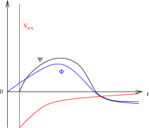
Fig. 13: (Color online) Radial dependence of the relative wave function $\Psi$ of two nucleons interacting via a hard-core potential $V_{NN}$. $\Phi$ refers to the uncorrelated wave function.

This point is more evident if we consider the extreme model of a hard-core potential, as is the case of the potential models developed in the early 1960s. This situation is illustrated in Fig. 13. For these potentials the perturbation expansion of the effective interaction in terms of $V_{NN}$ is meaningless, since each term of the series involving matrix elements of the $NN$ potential between unperturbed two-body states is infinite. This is because the unperturbed wave function, in contrast to the true wave function, gives a non-zero probability of finding a particle located inside the hard-core distance.

The traditional way out of this problem is the so-called Brueckner reaction matrix $G$, which is based on the idea of treating exactly the interaction between a given pair of nucleons [131]. The $G$ matrix, defined as a sum of all ladder-type interactions (see Sec. 4.1.2), is used to replace the $NN$ interaction vertices once a rearrangement of the effective interaction perturbative series has been performed.

Recently, a new method to renormalize the $NN$ interaction has been proposed [42, 43]. A low-momentum model space defined up to a cutoff momentum $\Lambda$ is introduced and an effective potential $V_{\rm low-k}$ is derived from $V_{NN}$. This $V_{\rm low-k}$ satisfies a decoupling condition between the low- and high-momentum spaces. Moreover, it is a smooth potential which preserves exactly the on-shell properties of the original potential and it is thus suitable to advantageously replace $V_{NN}$ in realistic many-body calculations.

Secs. 4.1 and 4.2 are devoted to the description of the reaction $G$ matrix and $V_{\rm low-k}$ potential, respectively.

Before doing this, however, it may be worth recalling that a method to avoid the $G$-matrix treatment to eliminate effects of the repulsive core in the $NN$ potential was proposed in the late 1960s [132, 40]. As already mentioned in the Introduction, this consists in using the experimental $NN$ phase shifts to deduce matrix elements of the $NN$ potential in a basis of relative harmonic oscillator states. These matrix elements, which have become known as the Sussex matrix elements (SME), have been used in several nuclear structure calculations, but the agreement with experiment has been generally only semi-quantitative. A comparison between the results obtained by Sinatkas et al. [133] using the SME and those obtained with a realistic effective interaction derived from the Bonn A potential is made for the N=50 isotones in [134].

4.1 The Brueckner $G$-matrix approach

4.1.1 Historical introduction

The concept of $G$ matrix originates from the theory of multiple scattering of Watson [135, 136]. In this approach, the elastic scattering of a fast particle by a nucleus was described by way of a transformed potential obtained in terms of the Lippmann-Schwinger matrix [137] for the two-body scattering. The procedure of Watson for constructing such an “equivalent two-body potential” was generalized to the study of nuclear many-body systems by Brueckner and co-workers [131, 138]. They introduced a reaction matrix for the scattering of two nucleons while they are moving in the nuclear medium. This matrix, which is known as the Brueckner reaction matrix, includes all two-particle correlations via summing all ladder-type interactions, and made it possible to perform Hartree-Fock self-consistent calculations for nuclear matter.

Only a few years later Goldstone [122] proved a new perturbation formula for the ground-state energy of nuclear matter which gave the formal basis of the Brueckner theory. The Goldstone linked-diagram theory applies to systems with non-degenerate ground state, which is the case of nuclear matter as well as of closed-shell finite nuclei.

The Brueckner theory was seen to be the key to solve the paradox on which the attention of many nuclear physicists was focused during the early 1950s. In fact, it allowed to reconcile a description of the nucleus in terms of an overall potential and the peculiar features of the two-body nuclear force. This was very well evidenced in the paper by Bethe [139], whose main purpose was indeed to establish that the Brueckner theory provided the theoretical foundation for the shell model.

After their first works, Brueckner and co-workers published a series of papers on the same subject [140, 141, 142, 143, 144], where further analyses and developments of the method as well as numerical calculations were given. Important advances as regards nuclear matter were provided by the work of Bethe and Goldstone [145] and Bethe et al. [146]. For several years up to the 1960s, nuclear physicists were indeed very active in this field, as may be seen from the review papers by Day [147], Rajaraman and Bethe [148], and Baranger [149], where comprehensive lists of references can be found. For a recent review of the developments in this area made Bethe and coworkers we refer to [150].

As regards open-shell nuclei, we have shown in the previous section that the model-space effective interaction may be obtained by way of a linked-diagram expansion containing both folded and non-folded Goldstone diagrams. An order-by-order perturbative calculation of such diagrams in terms of $V_{NN}$ is not appropriate and one has to resort again to the reaction matrix $G$.

The renormalization of $V_{NN}$ through the Brueckner theory has been the standard procedure to derive realistic effective interactions since the pioneering works of the early 1960s. A survey of shell-model calculations employing the $G$ matrix is given in Secs. 5.1 and 5.2.

In Sec. 4.1.2 we shall define the reaction matrix $G$ and discuss the main problems related to its definition. Then, in Sec. 4.1.3, we shall address the problem of how the reaction matrix may be calculated, focusing attention on the $G_{T}$ matrix for which plane waves are used as intermediate states. It is, in fact, this matrix which is most commonly used nowadays in realistic shell-model calculations. For simplicity, almost everywhere in this section we shall denote the $NN$ potential by $V$.

4.1.2 Essentials of the theory

In the literature, the $G$ matrix is typically introduced by way of the Goldstone expansion for the calculation of the ground-state energy in nuclear matter and closed shell nuclei. As a first step, the ground-state energy is written as a linked-cluster perturbation series. Then, all diagrams differing one from another only in the number of $V$ interactions between two particles lines are summed. This corresponds to define a well-behaved two-body operator, the reaction matrix $G$, that replaces the potential $V$ in the series. A very clear and simple presentation of the $G$ matrix along this line is provided in the paper by Day [147].

Here, we shall not discuss the details of the $G$-matrix theory, but simply give the elements needed to make clear its definition in connection with the derivation of the model-space effective interaction for open-shell nuclei. Therefore, in the following we refer, as in the previous section, to an $A$-nucleon system with the Hamiltonian given by Eqs. (7)-(9) and represented as a doubly closed core plus valence nucleons moving in a limited number of SP orbits above the core.

The two-body operator $G$ is defined by the integral equation

$$G(\omega)=V+V\frac{Q_{2p}}{\omega-H_{0}}G(\omega),$$ (77)

where $\omega$ is an energy variable known as “starting energy” and $Q_{2p}$ an operator which projects onto particle-particle states, namely states composed of two SP levels above the doubly closed core. As we shall discuss later, this operator may be chosen in different ways depending on the specific context in which it is used. Here it is worth noting that its presence in Eq. (77) reminds us that the $G$ matrix, differently from the Lippmann-Schwinger $T$ matrix, is defined in the nuclear medium. It may be also noted that the starting energy $\omega$ is not a free parameter. Rather, its value is determined by the physical problem being studied. For the $T$ matrix, $\omega$ denotes the scattering energy for two particles in free space, but depends on the nuclear medium for the $G$ matrix. In fact, we shall see that for a $G$ matrix to be used within the linked-diagram expansion of the effective interaction $\omega$ depends on the diagram where $G$ appears. Only in some cases it represents the energy of the two-particle incoming state, which was instead the meaning of the energy variable $\omega$ used in Sec. 3.

Let us start by writing the $Q_{2p}$ operator as

$$Q_{2p}=\sum_{ij}C(ij)|\phi_{ij}\rangle\langle\phi_{ij}|,$$ (78)

where the state $|\phi_{ij}\rangle$, which is the antisymmetrized product of the two SP states $|i\rangle$ and $|j\rangle$, is an eigenstate of $H_{0}$ with energy $\epsilon_{i}+\epsilon_{j}$. The constant $C(ij)$ is 1 if the state $|\phi_{ij}\rangle$ pertains to the space defined by $Q_{2p}$, 0 otherwise. We now introduce the operator $P_{2p}$ which projects on the complementary space

$$P_{2p}=1-Q_{2p}.$$ (79)

Taking matrix elements of $G$ between states of the $P_{2p}$-space we have

$$\langle\phi_{kl}|G(\omega)|\phi_{nm}\rangle=\langle\phi_{kl}|V|\phi_{nm}\rangle+\sum_{ij}\langle\phi_{kl}|V|\phi_{ij}\rangle\frac{C(ij)}{\omega-\epsilon_{i}-\epsilon_{j}}\langle\phi_{ij}|G(\omega)|\phi_{nm}\rangle,$$ (80)

which in a series expansion form becomes

$$\langle\phi_{kl}|G(\omega)|\phi_{nm}\rangle = \langle\phi_{kl}|V|\phi_{nm}\rangle+\sum_{ij}\langle\phi_{kl}|V|\phi_{ij}\rangle\frac{C(ij)}{\omega-\epsilon_{i}-\epsilon_{j}}\langle\phi_{ij}|V|\phi_{nm}\rangle$$ (81)

$$+\sum_{iji^{\prime}j^{\prime}}\langle\phi_{kl}|V|\phi_{ij}\rangle\frac{C(ij)}{\omega-\epsilon_{i}-\epsilon_{j}}\langle\phi_{ij}|V|\phi_{i^{\prime}j^{\prime}}\rangle\frac{C(i^{\prime}j^{\prime})}{\omega-\epsilon_{i^{\prime}}-\epsilon_{j^{\prime}}}\langle\phi_{i^{\prime}j^{\prime}}|V|\phi_{nm}\rangle+\cdots$$

The above expansion can be represented diagrammatically by the series shown in Fig. 14. The diagrams on the r.h.s. of this figure are known as “ladder” diagrams and each diagram corresponds to a situation in which a pair of particles interacts a certain number of times with the restriction that the intermediate states involved in the scattering must be those defined through the $Q_{2p}$ operator. In other words, two particles initially in a state of the $P_{2p}$-space undergo a sequence of scatterings into states of the $Q_{2p}$-space and then after several such scatterings go back to a state of the original space.

Fig. 14: Diagrammatic representation defining the matrix $G$.

For the sake of completeness, we introduce the correlated wave function $|\psi_{nm}(\omega)\rangle$ [145],

$$|\psi_{nm}(\omega)\rangle=|\phi_{nm}\rangle+\frac{Q_{2p}}{\omega-H_{0}}V|\psi_{nm}(\omega)\rangle,$$ (82)

which once iterated becomes

$$|\psi_{nm}(\omega)\rangle=|\phi_{nm}\rangle+\frac{Q_{2p}}{\omega-H_{0}}G(\omega)|\phi_{nm}\rangle,$$ (83)

where use has been made of the integral equation (77). Eq. (83) allows one to write the action of $G$ on an unperturbed state as

$$G(\omega)|\phi_{nm}\rangle=V|\psi_{nm}(\omega)\rangle,$$ (84)

which makes evident that the $G$ operator may be considered an effective potential. The correlated wave function (82) and its properties are extensively discussed in Refs. [149, 151, 152].

At this point, we go further in our discussion clarifying the meaning of the starting energy $\omega$ and illustrating some possible choices of the projection operator $Q_{2p}$.

Fig. 15: A graph of the projection operator $Q_{2p}$ appropriate for open-shell nuclei.

Let us begin with $Q_{2p}$. We define the $Q_{2p}$ operator by specifying its boundaries labelled by the three numbers ($n_{1}$,$n_{2}$,$n_{3}$), each representing a SP level, the levels being numbered starting from the bottom of the potential well. Explicitly, using Eq. (78) the operator $Q_{2p}$ is written as

$$C(ij)=\left\{\begin{array}[]{ll}1&\mbox{if $i,j>n_{2}$}\\ 1&\mbox{if $n_{1}<i\leq n_{2}$ and $j>n_{2}$}\\ {}&~{}~{}~{}~{}~{}~{}~{}~{}\mbox{or vice-versa}\\ 0&\mbox{otherwise.}\end{array}\right.$$

The graph of Fig. (15) makes more clear its definition. Note that the index $n_{3}$ denotes the number of levels in the full space. In principle, it should be infinite; in practice, as we shall see in Sec. 4.1.3, it is chosen to be a large but finite number. As regards the indices $n_{1}$ and $n_{2}$, the only mandatory requiriment is that none of them should be below the last occupied orbit of the doubly closed core. It is customary to take for $n_{1}$ the number the SP levels below the Fermi surface while $n_{2}$ may be chosen starting from the last SP valence level and going up. How this choice is performed is better illustrated by an example.

Let us consider the nucleus ¹⁸O which in the shell-model framework is described as consisting of the doubly closed ¹⁶O and two valence neutrons which are allowed to occupy the three levels of the $sd$ shell. The model-space effective interaction for ¹⁸O may be derived by using the linked-diagram expansion of Sec. 3, with the $G$ matrix replacing the $NN$ potential in all the irreducible, valence-linked diagrams composing the $\hat{Q}$-box. In so doing, one has to be careful to exclude from the $\hat{Q}$-box those diagrams containing a ladder sequence already included in the $G$ matrix. We may take the matrix $G$ with a $Q_{2p}$ operator as specified, for instance, by $(3,6,\infty)$. In this case, one of two SP levels composing the intermediate state in the calculation of the $G$ matrix has to be beyond the $sd$ shell while the other one may be also an $sd$ level. Then, when calculating the $\hat{Q}$-box the included diagrams strictly depend on the considered $G$ matrix. As an example, we have reported in Fig. 16 a first- and second-order diagram of the $\hat{Q}$-box, the wavy lines denoting the $G$-interactions. As discussed in Sec. 3.2.2, the incoming and outcoming lines of the A and B diagrams are levels of the $sd$ shell, while the the intermediate state of diagram B should have at least one passive line. This means that none of the two SP states, $x$ or $y$, could be a $0s$ or a $0p$ level and at least one of them must be beyond the $sd$ shell. Therefore, if we take the $G$ matrix with the $(3,6,\infty)$ $Q_{2p}$ operator, all possible B diagrams of Fig. 16 are already contained in the A diagram. On the other hand, if we increase the $n_{2}$ using a $G$ matrix with the $(3,10,\infty)$ $Q_{2p}$ operator, the B diagrams should explicitly appear in the calculation of the $\hat{Q}$-box providing that $x,y\leq 10$ and $x$ and/or $y\geq 7$. A detailed discussion on the points illustrated here is in Ref. [153].

Fig. 16: Second-order ladder diagram contained in the $\hat{Q}$-box.

We now come to the energy variable $\omega$ which may be seen as the “starting energy” at which $G$ is computed. We know that any $G$-vertex in a $\hat{Q}$-box diagram is employed as the substitute for the ladder series of Fig. 14 and therefore the corresponding starting energy depends on the diagram as a whole and in particular on the location of the $G$-vertex in the diagram. For instance, the $G$ matrices in the three vertices of diagrams A and B of Fig. 16 have to be calcutated at $\omega=\epsilon_{k}+\epsilon_{l}$, corresponding to the energy of the two-particle incoming state. As an other example, we have shown in Fig. 17 the diagram A. To illustrate how $\omega$ is evaluated we have written it as the sum of the ladder sequence A1, A2,…,A$n$,…. The lowest vertex of diagram A corresponds to $\langle\phi_{mp}|G(\omega)|\phi_{kh}\rangle$ and its starting energy can be determined by looking at the two lowest vertices in diagram A2 whose contribution may be written as

$$\frac{\langle\phi_{mp}|V|\phi_{xy}\rangle\langle\phi_{xy}|V|\phi_{kh}\rangle}{\epsilon_{k}+\epsilon_{h}-\epsilon_{x}-\epsilon_{y}}~{}~{}.$$ (85)

Note that the energy denominator of the $G$ matrix is given by $\omega-H_{0}$, $H_{0}$ acting on the intermediate two-particle state $|\phi_{xy}\rangle$. Therefore, to obtain the denominator of Eq. (85) as $\omega-\epsilon_{x}-\epsilon_{y}$, one has to choose $\omega=\epsilon_{k}+\epsilon_{h}$. Similarly, for the upper $G$-vertex of diagram A $\omega=\epsilon_{k}+\epsilon_{l}+\epsilon_{h}-\epsilon_{m}$. In both the previous examples $\omega$ is different from the energy of the incoming state, which results to be $\epsilon_{k}+\epsilon_{l}$.

In concluding this subsection it is important to consider the dependence of the $G$ matrix on the SP potential $U$, which explicitly appears in the denominator through $H_{0}$. The advantages of different choices have been extensively investigated essentially in connection with the Goldstone expansion and its convergence properties (see the review paper by Baranger [149]).

Fig. 17: Illustration of the summation procedure to replace $V$ vertices with $G$ vertices.

It is worth recalling that, as a general rule, in a perturbation approach to nuclear structure calculations one starts by summing and subtracting the SP potential $U$ to the Hamiltonian so as to have as perturbation $H_{1}=V-U$. As a consequence, the diagrams of the $\hat{Q}$-box for the shell-model effective interaction contain $-U$ as well as $V$ vertices. Diagrams where $-U$ vertices are attached to particle lines between successive $V$ interactions may be taken into account directly through the reaction matrix. This means that each diagram of the expansion shown in Fig. 14 is replaced with a new diagram in which any number of $-U$ insertions has been introduced in the particle lines. A typical diagram is shown in Fig. 18. In this way, a new reaction matrix may be introduced where the $-U$ interactions for the intermediate particle states are summed up to all orders. More precisely, by changing the propagator of the particle lines from $H_{0}$ to $H_{0}-Q_{2p}UQ_{2p}$ one obtains the reaction matrix with plane waves as intermediate states, which is usually called $G_{T}$. Note that the term $Q_{2p}UQ_{2p}$ instead of $U$ is subtracted from $H_{0}$ since, as pointed out in [149], particle and hole states are defined with respect to the SP potential $U$. In other words, the Hamiltonian $H_{0}-Q_{2p}UQ_{2p}$, which commutes with $Q_{2p}$, preserves the particle and hole states as defined by $U$. The reaction matrix $G_{T}$ satisfies the integral equation

$$G_{T}(\omega)=V+VQ_{2p}\frac{1}{\omega-Q_{2p}tQ_{2p}}Q_{2p}G_{T}(\omega),$$ (86)

where one has to recall that $t$ represents the kinetic energy.

An extensive study of the properties and features of $G_{T}$ in the framework of the shell model can be found in [153], where arguments in favor of the use of $G_{T}$ are given. We find it interesting to briefly recall these arguments here.

First of all, the $G_{T}$ matrix of Eq. (86) minimizes the dependence on the SP potential. In fact, it depends only on $Q_{2p}$ while the reaction matrix $G$ of Eq. (77) depends also on the spectrum of the SP states of the $Q_{2p}$ space.

Fig. 18: Typical $U$ insertions to the $G$-matrix intermediate states.

The second argument is essentially based on the paper by Bethe et al. [146], where it was shown that all $-U$ and Brueckner-Hartree-Fock self-energy insertions cancel each other when the self-energy is calculated on energy shell. This result may be plausibly extended [153] to low-energy intermediate particle states not far off the energy shell, but such a cancellation is very unlikely for the high-energy states. On the other hand, in nuclear matter calculations [152] it has been shown that the sum of self-energy-insertion diagrams and other three-body clusters is almost negligible, in other words they tend to cancel each other. If we assume that this nuclear-matter result still holds for finite nuclei, we reasonably expect that only the $-U$ insertions survive for high-energy intermediate states, so leading to the reaction matrix $G_{T}$. The use of the $G$ matrix of Eq. (77) is instead suggested for low-lying states assuming that $-U$ and Brueckner-Hartree-Fock self-energy insertions cancel approximately. In other words the reaction matrix calculation may be performed following a two-step procedure, which is discussed in detail in [153]. Here we only give a sketch of such procedure.

Let us start by dividing the intermediate states of the $Q_{2p}$ space into high-energy and low-energy states, the $Q_{2p}$ operator being written as

$$Q_{2p}=Q_{2p}^{h}+Q_{2p}^{l},$$ (87)

with orthogonalized plane waves used for $Q_{2p}^{h}$ and harmonic oscillator wave functions for $Q_{2p}^{l}$. The fist step consists in the calculation of the $G_{T}$ matrix of Eq. (86) with the projection operator taken as $Q_{2p}^{h}$. Then using this reaction matrix instead of the $NN$ potential the $G$ matrix of Eq. (77) is calculated with a projection operator restricted to $Q_{2p}^{l}$. Actually, the second step is carried out by means of a pertubative expansion which implies that the final reaction matrix, which we call $\tilde{G}_{T}$, is written as

$$\tilde{G}_{T}(\omega)=G_{T}(\omega)+G_{T}(\omega)\frac{Q_{2p}^{l}}{\omega-H_{0}}G_{T}(\omega)+G_{T}(\omega)\frac{Q_{2p}^{l}}{\omega-H_{0}}G_{T}(\omega)\frac{Q_{2p}^{l}}{\omega-H_{0}}G_{T}(\omega)+\cdots$$ (88)

Hence $\tilde{G}_{T}$ is obtained by summing to $G_{T}$ the second -, third-, $\cdots$ order two-particle ladder diagrams with $G_{T}(\omega)$ vertices and intermediate states restricted to the low-lying states defined by the $Q_{2p}^{l}$ operator. These ladder terms may be directly included in the evaluation of the $\hat{Q}$-box once the $G_{T}$ of Eq. (86) with $Q_{2p}^{h}$ as projection operator has been calculated. Note that in so doing no $-U$ or Brueckner-self-energy insertions are explicitly included in the $\hat{Q}$-box diagrams since, on the basis of the previous arguments, one may assume that they cancel each other.

It is worth to point out that no firm criteria exist on how to perform the partition of Eq. (87). It is customary to take $n_{2}$ in the definition of the $Q_{2p}^{h}$ operator so that it encompasses the shell above the model space [153]. For example, if we consider again ¹⁸O we specify $Q_{2p}$ by $(3,10,\infty)$ to define the $G_{T}$ matrix, then $Q_{2p}^{l}$ while corresponds to the $1p0f$-shell and the ladder terms with two particle in this shell are taken into account directly when the $\hat{Q}$-box is evaluated.

4.1.3 Calculation of the reaction matrix

Starting from the introduction of the $G$ matrix, several approximate techniques have been developed for the solution of Eq. (77) A review of them together with a critical discussion can be found in [147, 149, 45, 154]. Among the early methods we would just like to mention the separation method of Moszkowski and Scott [155] and the reference spectrum method of Bethe et al. [146], which have both been extensively applied to both nuclear matter and finite nuclei. For many years, they were the primary methods for $G$-matrix calculation and were first employed by Kuo and Brown [18] to calculate from the Hamada-Johnston potential [63] the $G$ matrix elements to be used in shell-model calculations for ¹⁸O and ¹⁸F. It is interesting to note that during the 1970s significant advances were made in the calculation of the reaction matrix as regards the $G$ matrix of Eq. (77) with harmonic oscillator intermediate states as well as the $G_{T}$ matrix of Eq. (86) having plane-wave intermediate states. In fact, accurate solutions of Eq. (77) were proposed by Barrett et al. [156] and of Eq. (86) by Tsai and Kuo [36], both of them providing an exact treatment of the projection operator $Q_{2p}$.

Here we shall only focus on the technique to compute the reaction matrix of Eq. (86), which we have used in our shell-model calculations. More precisely, we shall describe the method proposed by Tsai and Kuo [36], which was further investigated and applied by Krengiglowa et al. [153]. This method, based on a matrix inversion in the momentum space, allows, as mentioned above, an exact treatment of the projection $Q_{2p}$ operator except for the only approximation of using a finite value instead of infinity for $n_{\rm 3}$ defining $Q_{2p}$.

Let us start by noting that a solution of Eq. (86) is

$$G_{T}(\omega)=V+VQ_{2p}\frac{1}{Q_{2p}(e-V)Q_{2p}}Q_{2p}V,$$ (89)

as it can be easily shown using the operator identity

$$\frac{1}{A-B}=\frac{1}{A}+\frac{1}{A}B\frac{1}{A-B}~{},$$ (90)

with $e=\omega-t$, $A=Q_{2p}~{}e~{}Q_{2p}$, and $B=Q_{2p}VQ_{2p}$.

The propagator of Eq. (89) was shown [36] to take the form

$$Q_{2p}\frac{1}{Q_{2p}(e-V)Q_{2p}}Q_{2p}=\frac{1}{e-V}-\frac{1}{e-V}P_{2p}\frac{1}{P_{2p}\frac{1}{e-V}P_{2p}}P_{2p}\left.\frac{1}{e-V}\right.,$$ (91)

where $P_{2p}$ is defined in Eq. (79) . The identity (91) allows us to rewrite Eq. (89) as

$$G_{T}(\omega)=G_{TF}(\omega)+\Delta G(\omega),$$ (92)

with

$$\Delta G(\omega)=-V\frac{1}{e-V}P_{2p}\frac{1}{P_{2p}\frac{1}{e-V}P_{2p}}P_{2p}\frac{1}{e-V}V$$ (93)

and

$$G_{TF}(\omega)=V+V\frac{1}{e-V}V=V+V\frac{1}{e}G_{TF}(\omega),$$ (94)

where we have used the identity (90) with $Q_{2p}=1$ to obtain relation (94).

An equivalent and very convenient expression of $\Delta G(\omega)$ which has also the advantage to be applicable when $V$ is a hard-core potential is

$$\Delta G(\omega)=-G_{TF}(\omega)\frac{1}{e}P_{2p}\frac{1}{P_{2p}[(1/e)+(1/e)G_{TF}(1/e)]P_{2p}}P_{2p}\frac{1}{e}G_{TF}(\omega).$$ (95)

The set of Eqs. (92, 94, 95) provides a very convenient way to calculate the $G_{T}$ matrix once a finite-$n_{3}$ approximation is made, namely a truncated $P_{2p}$-space is taken. Let us define

$$G_{R}(\omega) = G_{TF}(1/e),$$

$$G_{L}(\omega) = (1/e)G_{TF},$$

$$G_{LR}(\omega) = (1/e)+(1/e)G_{TF}(1/e),$$ (96)

then Eq. (92) in a matrix formalism can be written as

$$\langle\phi_{kl}|G_{T}(\omega)|\phi_{lm}\rangle=\langle\phi_{kl}|G_{TF}(\omega)|\phi_{lm}\rangle-\sum_{ijkl\in P_{2p}}\langle\phi_{kl}|G_{L}(\omega)|\phi_{ij}\rangle\times\langle\phi_{ij}|G^{-1}_{LR}(\omega)|\phi_{kl}\rangle\langle k~{}l|G_{R}(\omega)|\phi_{lm}\rangle~{}.$$ (97)

This equation makes clear the necessity of a finite-$n_{3}$ approximation. In fact, the $G^{-1}_{LR}$ matrix appearing in this equation is defined in the $P_{2p}$ space and represents the inverse of the $P_{2p}G_{LR}P_{2p}$ matrix, which has to be a finite matrix.

The basic ingredient for the calculation of the $G_{T}$ matrix through Eq. (92) is the matrix $G_{TF}$ which is identical to the $G_{T}$ defined by Eq. (86), except that is free from the projection operator $Q_{2p}$. A very convenient way to calculate $G_{TF}(\omega)$ is to employ the momentum-space matrix inversion method [157]. Once the $G_{TF}$ matrix elements in the momentum space are known, the matrices $G_{L}$, $G_{R}$, and $G_{LR}$ can be easily evaluated in the same space. As a final step, these matrices are all transformed in the harmonic oscillator basis and the $G_{T}$ matrix is obtained by means of Eq. (97) though simple matrix operations.

Here we have only given a sketch of the procedure to solve Eqs. (92), (94), (95). A detailed description of the whole procedure can be found in [153], where the validity of an $n_{3}$-finite approximation is discussed. It is worth mentioning that this point is also discussed in Ref. [45].

4.2 The $V_{\rm low-k}$ approach

In this subsection we shall describe in detail the derivation and main features of the low-momentum $NN$ interaction $V_{\rm low-k}$, which has been introduced in Refs. [42, 43, 44]. The idea underlying the construction of $V_{\rm low-k}$ from a realistic model for $V_{NN}$ is based on the renormalization group (RG) and the effective field theory (EFT) approaches [158, 92, 90, 91]. As mentioned in Sec. 2, while the high-quality $NN$ potentials all reproduce the empirical deuteron properties and low-energy phase shifts very accurately, they differ significantly from one another in the high momentum behavior. A cutoff momentum $\Lambda$ that separates fast and slow modes is then introduced and from the original $V_{NN}$ an effective potential $V_{\rm low-k}$, satisfying a decoupling condition between the low- and high-momentum spaces, is derived by integrating out the high-momentum components. The main result is that $V_{\rm low-k}$ is free from the model-dependent high-momentum modes. In consequence, it is a smooth potential which preserves exactly the onshell properties of the original $V_{NN}$, and is suitable to be used directly in nuclear structure calculations. In Sec. 5.3.1, we will show that the $V_{\rm low-k}$ approach provides a real alternative to the Brueckner $G$-matrix renormalization procedure.

4.2.1 Derivation of the low-momentum $NN$ potential 1 $V_{\rm low-k}$

In carrying out the above high-momentum integration, or decimation, an important requirement is that the low-energy physics of $V_{NN}$ is exactly preserved by $V_{\rm low-k}$. For the two-nucleon problem, there is one bound state, namely the deuteron. Thus one must require that the deuteron properties given by $V_{NN}$ are preserved by $V_{\rm low-k}$. In the nuclear effective interaction theory, there are several well-developed model-space reduction methods. One of them is the Kuo-Lee-Ratcliff (KLR) folded diagram method [121, 38], which was originally formulated for discrete (bound state) problems. A detailed discussion of this method has been given earlier in Sec. 3.

For the two-nucleon problem, we want the effective interaction $V_{\rm low-k}$ to preserve also the low-energy scattering phase shifts, in addition to the deuteron binding energy. Thus we need an effective interaction for scattering (unbound) problems. A convenient framework for this purpose is the $T$-matrix equivalence approach, as described below.

We use a continuum model space specified by

$$P=\int d\mbox{\boldmath$p$}\mid\mbox{\boldmath$p$}\rangle\langle\mbox{\boldmath$p$}\mid~{},~{}~{}~{}~{}p\leq\Lambda$$ (98)

where $p$ is the two-nucleon relative momentum and $\Lambda$ the cutoff momentum which is also known as the decimation momentum. Its typical value is about 2 fm^-1 as we shall discuss later. Our purpose is to look for an effective interaction $PV_{\rm eff}P$, with $P$ defined above, which preserves certain properties of the full-space interaction $V_{NN}$ for both bound and unbound states. This effective interaction is referred to as $V_{\rm low-k}$.

We start from the full-space half-on-shell $T$-matrix (written in a single partial wave channel)

$$T(k^{\prime},k,k^{2})=V_{NN}(k^{\prime},k)+\mathcal{P}\int_{0}^{\infty}q^{2}dqV_{NN}(k^{\prime},q)\frac{1}{k^{2}-q^{2}}T(q,k,k^{2}).$$ (99)

This is the $T$-matrix for the two-nucleon problem with the Hamiltonian

$$H=H_{0}+V_{NN}=t+V_{NN}~{},$$ (100)

$t$ being the relative kinetic energy. We then define a $P$-space low-momentum $T$-matrix by

$$T_{\rm low-k}(p^{\prime},p,p^{2})=V_{\rm low-k}(p^{\prime},p)+\mathcal{P}\int_{0}^{\Lambda}q^{2}dqV_{\rm low-k}(p^{\prime},q)\frac{1}{p^{2}-q^{2}}T_{\rm low-k}(q,p,p^{2}),$$ (101)

where $(p^{\prime},p)\leq\Lambda$ and the integration interval is from 0 to $\Lambda$. In the above, the symbol $\mathcal{P}$ in front of the integration sign denotes principal value integration. We require the equivalence condition

$$T(p^{\prime},p,p^{2})=T_{\rm low-k}(p^{\prime},p,p^{2});~{}(p^{\prime},p)\leq\Lambda.$$ (102)

The above equations define the effective low-momentum interaction; it is required to preserve the low-momentum ($\leq\Lambda$) half-on-shell $T$-matrix. Since phase shifts are given by the full-on-shell $T$-matrix $T(p,p,p^{2})$, low-energy phase shifts given by the above $V_{\rm low-k}$ are clearly the same as those of $V_{NN}$.

In the following, let us show that a solution of the above equations may be found by way of the KLR folded-diagram method [121, 38] described in Sec. 3 as a means to construct the shell-model effective interaction. Within this approach the $V_{\rm low-k}$ may be written in the operator form as

$$V_{\rm low-k}=\hat{Q}-\hat{Q^{\prime}}\int\hat{Q}+\hat{Q^{\prime}}\int\hat{Q}\int\hat{Q}-\hat{Q^{\prime}}\int\hat{Q}\int\hat{Q}\int\hat{Q}+~{}...~{},$$ (103)

which contains a $\hat{Q}$-box whose explicit definition is given below.

In the time-dependent formulation, the $T$-matrix of Eq. (99) can be written as $\langle k^{\prime}\mid VU(0,-\infty)\mid k\rangle$, $U(0,-\infty)$ being the time-evolution operator. In this way a diagrammatic analysis of the $T$-matrix can be made. A general term of $T$ may be written as

$$\langle k^{\prime}\mid\left[V+V\frac{1}{e(k^{2})}V+V\frac{1}{e(k^{2})}V\frac{1}{e(k^{2})}V+...\right]\mid k\rangle,$$ (104)

where $e(k^{2})\equiv(k^{2}-H_{0})$.

Note that the intermediate states (represented by 1 in the numerator) cover the entire space. In other words, we have $1=P+Q$ where $P$ denotes the model-space projection operator and $Q$ its complement. Expanding it out in terms of $P$ and $Q$, a typical term of $T$ is of the form

$$V\frac{Q}{e}V\frac{Q}{e}V\frac{P}{e}V\frac{Q}{e}V\frac{P}{e}V.$$ (105)

Let us now define the $\hat{Q}$-box as

$$\langle k^{\prime}\mid\hat{Q}(k^{2})\mid k\rangle=\langle k^{\prime}\mid\left[V+V\frac{Q}{e(k^{2})}V\right.+\left.V\frac{Q}{e(k^{2})}V\frac{Q}{e(k^{2})}V+...\right]\mid k\rangle,$$ (106)

where all intermediate states belong to $Q$. One readily sees that the $P$-space portion of the $T$-matrix can be regrouped in terms of a $\hat{Q}$-box series, more explicitly as

$$\langle p^{\prime}\mid T\mid p\rangle=\langle p^{\prime}\mid\left[\hat{Q}+\hat{Q}\frac{P}{e(p^{2})}\hat{Q}\right.\left.+\hat{Q}\frac{P}{e(p^{2})}\hat{Q}\frac{P}{e(p^{2})}\hat{Q}+...\right]\mid p\rangle.$$ (107)

Note that all the $\hat{Q}$-boxes have the same energy variable, namely $p^{2}$. This regrouping is shown in Fig. 19, where each $\hat{Q}$-box is denoted by a circle and the solid line represents the propagator $\frac{P}{e}$. The diagrams A, B and C are respectively the one- and two- and three-$\hat{Q}$-box terms of $T$, and clearly $T$=A+B+C+$\cdots$. Note that the dashed vertical line is not a propagator; it is just a “ghost” line to indicate the external indices.

Fig. 19: Folded-diagram factorization of the half-on-shell $T$-matrix.

Now a folded-diagram factorization for the $T$-matrix can be performed, following the same procedure as in Sec. 3 [121, 38]. As is discussed in Sec. 3.2.1, diagram B of Fig. 19 may be factorized into the product of two parts (see B1) where the time integrations of the two parts are independent from each other, each integrating from $-\infty$ to 0. In this way we have introduced a time-incorrect contribution which must be corrected. In other words, B is not equal to B1, rather it is equal to B1 minus the folded-diagram correction B2. Schematically the above factorization is written as

$$\hat{Q}\frac{P}{e}\hat{Q}=\hat{Q}\times\hat{Q}-\hat{Q}^{\prime}\int\hat{Q},$$ (108)

where the last term is the once-folded two $\hat{Q}$-box term. The meaning of the correction term B2 can also be visualized in terms of the differences in the $\hat{Q}$-box energy variables. With such energies explicitly written out, the above equation represents

$$\langle p^{\prime}\mid\hat{Q}(p^{2})\frac{P}{e(p^{2})}\hat{Q}(p^{2})\mid p\rangle=\sum_{p^{\prime\prime}}\langle p^{\prime}\mid\hat{Q}(p^{\prime\prime 2})\mid p^{\prime\prime}\rangle~{}~{}\langle p^{\prime\prime}\mid\frac{P}{e(p^{2})}\hat{Q}(p^{2})\mid p\rangle-\langle p^{\prime}\mid\hat{Q}^{\prime}\int\hat{Q}\mid p\rangle.$$ (109)

Note that the energy variable for the first $\hat{Q}$-box on the right hand side of this equation is $p^{\prime\prime 2}$ instead of $p^{2}$. Before factorization, the energy variable for this $\hat{Q}$-box is $p^{2}$. We recall that the integral sign represents a generalized folding operation and the leading $\hat{Q}$-box of any folded term must be at least of second order in $V_{NN}$.

In the same way, we factorize the three-$\hat{Q}$-box term C as shown in the third line of Fig. 19:

$$\hat{Q}\frac{P}{e}\hat{Q}\frac{P}{e}\hat{Q}=\hat{Q}\times\hat{Q}\frac{P}{e}\hat{Q}-[\hat{Q}^{\prime}\int\hat{Q}]\times\hat{Q}+\hat{Q}^{\prime}\int\hat{Q}\int\hat{Q},$$ (110)

Higher-order $\hat{Q}$-box terms are also factorized following the same folded-diagram procedure. Let us now collect the terms in the figure in a “slanted” way. The sum of terms A1, B2, C3… is just the low-momentum effective interaction of Eq. (103). The sum B1, C2, D3…. is $V_{\rm low-k}\frac{P}{e}\hat{Q}$. Similarly the sum C1+D2+E3+$\cdots$ is just $V_{\rm low-k}\frac{P}{e}\hat{Q}\frac{P}{e}\hat{Q}$. It is worth to mention that diagrams D1, D2, $\cdots$, E1, E2, $\cdots$ are not shown in Fig. 19. Continuing this procedure, it can be seen that the $P$-space portion of $T$-matrix is $V_{\rm low-k}+V_{\rm low-k}\frac{P}{e}T$. Namely, the $V_{\rm low-k}$ defined by Eq. (103) is a solution of Eqs. (99)-(102).

An advantageous method to calculate the series in Eq. (103) is the Lee-Suzuki one, as described in Sec. 3.3. Following this algebraic approach the $V_{\rm low-k}$ is expressed as

$$V_{\rm low-k}=PV_{NN}P+PV_{NN}Q\omega,$$ (111)

where the operator $\omega$ is given by the solution of the decoupling equation (70). Note that in this latter equation the letter $\Omega$ was used instead of $\omega$ to avoid confusion with the energy variable $\omega$ defined in the same section. Here, since there is no problem of ambiguity, the same letter of the original paper by Lee and Suzuki [129] has been used and, for the sake of clarity, Eq. (70) is re-written for the Hamiltonian (100)

$$QV_{NN}P+QHQ\omega-\omega PHP-\omega PV_{NN}Q\omega=0~{}~{}.$$ (112)

The iterative technique presented in Sec. 3.3 to solve the decoupling equation is formulated for degenerate model spaces. Therefore, it is not useful in this case since $PH_{0}P=PtP$ is obviously non-degenerate. We can then resort to the iterative technique for non-degenerate model spaces proposed by Andreozzi [159] to solve the decoupling equation [see Eq. (112)] of the Lee-Suzuki method. This procedure, which will be referred to the Andreozzi-Lee-Suzuki (ALS) procedure, is quite convenient for obtaining the low-momentum $NN$ interaction.

We give now a sketch of this procedure. Let us define the operators:

$$p(\omega) = PHP+PHQ\omega,$$ (113)

$$q(\omega) = QHQ-\omega PHQ,$$ (114)

in terms of which the basic equations of the ALS iterative procedure read

$$x_{0} = -(QHQ)^{-1}QHP,$$

$$x_{1} = q(x_{0})^{-1}x_{0}p(x_{0}),$$

$$~{}.~{}.~{}.$$

$$x_{n} = q(x_{0}+x_{1}+...+x_{n-1})^{-1}x_{n-1}p(x_{0}+x_{1}+...+x_{n-1}).$$ (115)

Once the iterative procedure has converged, $x_{n}\rightarrow 0$, [159], the operator $\omega$ is given by

$$\omega_{n}=\sum^{n}_{i=0}x_{i},$$ (116)

and the $V_{\rm low-k}$ is obtained by Eq. (111).

In applying the ALS method, we have employed a momentum-space discretization procedure by introducing an adequate number of Gaussian mesh points [153].

4.2.2 Phase-shift equivalent Hermitian $V_{\rm low-k}$’s

It should be pointed out that the low-momentum $NN$ interaction given by the above folded-diagram expansion is not Hermitian. This is not convenient for applications, and one would like to have an interaction which is Hermitian. We shall describe how a family of Hermitian $V_{\rm low-k}$’s can be derived if we relax the half-on-shell $T$-matrix preservation. This subject has been studied in [160], where a general framework for constructing hermitian effective interactions is introduced, and it is shown how this generates a family of hermitian phase-shift equivalent low-momentum $NN$ interactions.

In the following, we outline the essential steps for the derivation of a Hermitian $V_{\rm low-k}$. We denote the folded-diagram low-momentum $NN$ interaction obtained from the ALS procedure as $V_{LS}$. The model-space secular equation for $V_{LS}$ is

$$P(H_{0}+V_{LS})P|\chi_{m}\rangle=E_{m}|\chi_{m}\rangle,$$ (117)

where $\{E_{m}\}$ is a subset of the eigenvalues $\{E_{n}\}$ of the full-space Schrödinger equation, $(H_{0}+V)|\Psi_{n}\rangle=E_{n}|\Psi_{n}\rangle$, and $|\chi_{m}\rangle$ is the $P$-space projection of the full-space wave function $|\Psi_{m}\rangle$, namely $|\chi_{m}\rangle=P|\Psi_{m}\rangle$. The above effective interaction may be rewritten in terms of the wave operator $\omega$ [see Eqs.(66),(67), (68)]

$$PV_{LS}P=Pe^{-\omega}(H_{0}+V)e^{\omega}P-PH_{0}P.$$ (118)

While the full-space eigenvectors $|\Psi_{n}\rangle$ are orthogonal to each other, the model-space eigenvectors $|\chi_{m}\rangle$’s are clearly not so and consequently the effective interaction $V_{LS}$ is not Hermitian. We now make a $Z$ transformation such that

$$Z|\chi_{m}\rangle = |v_{m}\rangle;$$

$$\langle v_{m}\mid v_{m^{\prime}}\rangle = \delta_{mm^{\prime}};~{}~{}m,m^{\prime}=1,~{}d,$$ (119)

where $d$ is the dimension of the model space. This transformation reorients the vectors $|\chi_{m}\rangle$’s such that they become orthonormal. We assume that the $|\chi_{m}\rangle$’s are linearly independent so that $Z^{-1}$ exists, otherwise the above transformation is not possible. Since $|v_{m}\rangle$ and $Z$ exist entirely within the model space, we can write $|v_{m}\rangle=P|v_{m}\rangle$ and $Z=PZP$.

Using Eq. (119), we transform Eq. (117) into

$$Z(H_{0}+V_{LS})Z^{-1}|v_{m}\rangle=E_{m}|v_{m}\rangle,$$ (120)

which implies

$$Z(H_{0}+V_{LS})Z^{-1}=\sum_{m\epsilon P}E_{m}\mid v_{m}\rangle\langle v_{m}\mid.$$ (121)

Since $E_{m}$ is real (it is an eigenvalue of $(H_{0}+V)$ which is Hermitian) and the vectors $|v_{m}\rangle$ are orthonormal, $Z(H_{0}+V_{LS})Z^{-1}$ is clearly Hermitian. The non-Hermitian secular equation (117) is now transformed into a Hermitian model-space eigenvalue problem

$$P(H_{0}+V_{herm})P|v_{m}\rangle=E_{m}|v_{m}\rangle,$$ (122)

with the Hermitian effective interaction given by

$$V_{herm}=Z(H_{0}+V_{LS})Z^{-1}-PH_{0}P,$$ (123)

or equivalently

$$V_{herm}=Ze^{-\omega}(H_{0}+V)e^{\omega}Z^{-1}-PH_{0}P.$$ (124)

To calculate $V_{herm}$, we must first have the $Z$ transformation. Since there are certainly many ways to construct $Z$, this generates a family of Hermitian effective interactions, all originating from $V_{LS}$. For example, we can construct $Z$ using the familiar Schmidt orthogonalization procedure. We denote the hermitian effective interaction obtained using this $Z$ transformation as $V_{schm}$.

We can also construct $Z$ analytically in terms of the wave operator. From the properties of the wave operator $\omega$, we have

$$\langle\chi_{m}\mid(1+\omega^{+}\omega)\mid\chi_{m^{\prime}}\rangle=\delta_{mm^{\prime}}.$$ (125)

It follows that an analytic choice for the $Z$ transformation is

$$Z=P(1+\omega^{+}\omega)^{1/2}P.$$ (126)

This leads to the Hermitian effective interaction

$$V_{\rm okb}=P(1+\omega^{+}\omega)^{1/2}P(H_{0}+V_{LS})P(1+\omega^{+}\omega)^{-1/2}P-PH_{0}P,$$ (127)

or equivalently

$$V_{\rm okb}=P(1+\omega^{+}\omega)^{-1/2}(1+\omega^{+})(H_{0}+V)(1+\omega)(1+\omega^{+}\omega)^{-1/2}P-PH_{0}P.$$ (128)

This is just the Okubo Hermitian effective interaction [161]. The Hermitian effective interaction of Suzuki and Okamoto [162, 10] is equivalent to the above.

There is another interesting choice for the transformation $Z$. As pointed out in [159], the positive definite operator $P(1+\omega^{+}\omega)P$ admits the Cholesky decomposition, namely

$$P(1+\omega^{+}\omega)P=PLL^{T}P,$$ (129)

where $L$ is a lower triangular matrix, $L^{T}$ being its transpose. Since $L$ is real and within the $P$-space, we have

$$Z=L^{T},$$ (130)

and the corresponding Hermitian effective interaction from Eq. (123) is

$$V_{\rm chol}=PL^{T}P(H_{0}+V_{LS})P(L^{-1})^{T}P-PH_{0}P.$$ (131)

We have found that this Hermitization procedure is numerically more convenient than the other methods. In the practical applications presented in this review we have employed this procedure. From now on, we shall denote the Hermitian low-momentum $NN$ interaction as $V_{\rm low-k}$.

Using a solvable matrix model, it has been shown that the above Hermitian effective interactions $V_{\rm schm},V_{\rm okb}$, and $V_{\rm chol}$ can be in general quite different [160] from each other and from $V_{LS}$, especially when $V_{LS}$ is largely non-Hermitian. For the $V_{NN}$ case, it is fortunate that the $V_{\rm low-k}$ corresponding to $V_{LS}$ is only slightly non-Hermitian. As a result, the Hermitian low-momentum $NN$ interactions $V_{\rm schm},V_{\rm okb}$, and $V_{\rm chol}$ are all quite similar to each other and to the one corresponding to $V_{LS}$, as discussed in [160].

We have just shown that a family of Hermitian effective interactions $V_{\rm low-k}$’s can be generated starting from the Lee-Suzuki transformation. In the following, we shall prove that all such interactions preserve the full-on-shell $T$-matrix $T(p,p,p^{2})$, $p\leq\Lambda$, and consequently they are all phase-shift equivalent

Let us consider two $T$-matrices

$$T_{1}(p^{2})=V_{1}+V_{1}g(p^{2})T_{1}(p),$$ (132)

and

$$T_{2}(p^{\prime 2})=V_{2}+V_{2}g(p^{\prime 2})T_{2}(p^{\prime}),$$ (133)

which are defined starting from two different potentials, $V_{1}$ and $V_{2}$, and/or two different propagators, $g(p^{2})={\mathcal{P}}(p^{2}_{1}-H_{0})^{-1}$ and $g(p^{\prime 2})={\mathcal{P}}(p^{\prime 2}_{2}-H_{0})^{-1}$. These $T$-matrices are related by the well known two-potential formula [146]

$$T_{2}^{\dagger}(p^{\prime 2})=T_{1}(p^{2})+T_{2}^{\dagger}(p^{\prime 2})[g(p^{\prime 2})-g(p^{2})]T_{1}(p^{2})+X_{2}(p^{\prime 2})[V_{2}-V_{1}]X_{1}(p^{2}),$$ (134)

where the operator $X=e^{\omega}$ [see Eq. (66)] is defined so as to have $T=VX$.

Applying the above relation to the half-on-shell $T$-matrix elements in momentum space, we have

$$\langle p^{\prime}|T_{2}^{\dagger}(p^{\prime 2})|p\rangle=\langle p^{\prime}|T_{1}(p^{2})|p\rangle+\langle p^{\prime}|T_{2}^{\dagger}(p^{\prime 2})[g(p^{\prime 2})-g(p^{2})]T_{1}(p^{2})|p\rangle+\langle\psi_{2}(p^{\prime})|(V_{2}-V_{1})|\psi_{1}(p)\rangle.$$ (135)

Here the true and unperturbed wave functions are related by $|\psi_{1}(p)\rangle=X_{1}(p^{2})|p\rangle$ and similarly for $\psi_{2}$. Using the above relation, we shall now show that the phase shifts of the full-space interaction $V_{NN}$ are preserved by the Hermitian interaction $V_{\rm low-k}$ for momentum $\leq\Lambda$. Let us denote the last term of Eq. (135) as $D(p^{\prime},p)$. We use $V_{\rm low-k}$ for $V_{2}$ and $V_{NN}$ for $V_{1}$. Recall that the eigenfunction of $(H_{0}+V_{\rm low-k})$ is $|v_{m}\rangle$ [see Eq. (117)] and that for $H\equiv(H_{0}+V_{NN})$ is $|\Psi_{m}\rangle$. We define a wave operator

$$U_{P}=\sum_{m\in P}|v_{m}\rangle\langle\Psi_{m}|.$$ (136)

Then $|v_{m}\rangle=U_{P}|\Psi_{m}\rangle$ and $PV_{\rm low-k}P=U_{P}(H_{0}+V_{NN})U_{P}^{\dagger}-PH_{0}P$. For our present case, $\langle\psi_{2}(p^{\prime})|$ is $\langle v_{p^{\prime}}|$ and $|\psi_{1}(p)\rangle$ is $|\Psi_{p}\rangle$. Since $\langle v_{p^{\prime}}|U_{P}=\langle\Psi_{p^{\prime}}|$, we have

$$D(p^{\prime},p)=\langle\Psi_{p^{\prime}}|(HU_{P}^{\dagger}-U_{P}^{\dagger}H)|\Psi_{p}\rangle=(p^{\prime 2}-p^{2})\langle v_{p^{\prime}}|\Psi_{p}\rangle.$$ (137)

Clearly $D(p,p)=0$. The second term on the right hand side of Eq. (135) vanishes when $p^{\prime}=p$. Hence

$$\langle p|T_{\rm low-k}(p^{2})|p\rangle=\langle p|T(p^{2})|p\rangle,~{}p\leq\Lambda,$$ (138)

where $T_{\rm low-k}$ is the $T$-matrix for $(PH_{0}P+V_{low-k})$ and $T$ for $(H_{0}+V_{NN})$. Thus we have shown that the phase shifts of $V_{NN}$ are preserved by $V_{\rm low-k}$. Recall that our $T$-matrices are real, because of the principal-value boundary conditions employed.

4.2.3 Properties of $V_{\rm low-k}$

We have shown above that low-energy observables given by the full-momentum potential $V_{NN}$ are preserved by the low-momentum potential $V_{\rm low-k}$. This preservation is an important point, and it is worth checking numerically that the deuteron binding energy and low-energy phase shifts given by $V_{NN}$ are indeed reproduced by $V_{\rm low-k}$. In this subsection we would like to report some results in this regard, together with some discussion about the differences between the various modern potentials.

Before presenting the results, let us first address an important question concerning the choice of the momentum cutoff $\Lambda$ in the derivation of $V_{\rm low-k}$. Phase shifts are given by the full-on-shell $T$-matrix $T(p,p,p^{2})$, hence, for a chosen $\Lambda$, $V_{\rm low-k}$ can reproduce phase shifts up to $E_{lab}=2\hbar^{2}\Lambda^{2}/M$, $M$ being the nucleon mass. Realistic $NN$ potentials are constructed to fit empirical phase shifts up to $E_{lab}\approx 350$ MeV [85], which is the pion production threshold. It is reasonable then to require $V_{\rm low-k}$ to reproduce phase shifts also up to this energy. Thus one should use $\Lambda$ in the vicinity of 2 fm^-1.

Table 1: Calculated binding energies $BE_{d}$ of the deuteron (MeV) for different values of the cutoff $\Lambda$ (fm^-1). The $V_{\rm low-k}$ has been calculated from the CD-Bonn potential for which $BE_{d}=2.224575$ MeV [88].

$\Lambda$	0.5	1.0	1.5	2.0	2.5	3.0
	2.2246	2.2246	2.2246	2.2246	2.2246	2.2246

We first check the deuteron binding energy $BE_{d}$ given by $V_{\rm low-k}$. For a range of $\Lambda$, such as 0.5 fm${}^{-1}\leq\Lambda\leq 3$ fm^-1, $BE_{d}$ given by $V_{\rm low-k}$ agrees very accurately (to 4 places after the decimal point) with that given by $V_{NN}$. In Table 1, we present the results for the $V_{\rm low-k}$ derived from the CD-Bonn $NN$ potential [88].

We have also checked the phase shifts and the half-on-shell $T(p^{\prime},p,p^{2})$ matrix elements with $(p^{\prime},p)\leq\Lambda$.

In Table 2 we report the neutron-proton ${}^{1}S_{0}$ phase shifts calculated both with the CD-Bonn potential and its $V_{\rm low-k}$ (with a cutoff momentum $\Lambda=2~{}{\rm fm}^{-1}$). It is worth noting that the degree of accuracy shown in Table 2 allows $V_{\rm low-k}$ to reproduce the $\chi^{2}/datum$ of the original potential up to $E_{\rm lab}=2\hbar^{2}\Lambda^{2}/M$.

Table 2: $np$ ${}^{1}S_{0}$ phase shifts (deg) as predicted by the CD-Bonn potential and its $V_{\rm low-k}$ ($\Lambda=2.0~{}{\rm fm}^{-1}$).

$E_{\rm lab}$	CD-Bonn	$V_{\rm low-k}$	Expt.
1	62.1	62.1	62.1
10	60.0	60.0	60.0
25	50.9	50.9	50.9
50	40.5	40.5	40.5
100	26.4	26.4	26.8
150	16.3	16.3	16.9
200	8.3	8.3	8.9
250	1.6	1.6	2.0
300	-4.3	-4.3	-4.5

In Table 3, for sake of completeness, we present also the deuteron quadrupole moments for different values of the cutoff momentum $\Lambda$, calculated with the corresponding $V_{\rm low-k}$’s, derived from the Argonne $V_{18}$ potential. These values are compared with the one predicted by the original potential.

Table 3: Deuteron quadrupole moments (fm²) as predicted by the Argonne $V_{18}$ potential and its $V_{\rm low-k}$ for different values of $\Lambda$ (fm^-1)

Argonne $V_{18}$	$\Lambda$	$V_{\rm low-k}$
0.270	1.8	0.268
	2.0	0.269
	2.2	0.270
	2.4	0.270
	2.6	0.270
	2.8	0.270

In Figs. 20 and 21 we compare $np$ ${}^{1}S_{0}$ $T(p^{\prime},p,p^{2})$ matrix elements given by the CD-Bonn potential and its $V_{\rm low-k}$ with a cutoff momentum $\Lambda=2.0$ fm^-1 and $p=0.35,~{}1.34$ fm^-1. From these figures it can be seen that, even if the half-on-shell $T$-matrix is not exactly preserved by the ALS transformation, it is reproduced to a good degree of accuracy.

Fig. 20: (Color online) Comparison of the half-on-shell $T(p^{\prime},p,p^{2})$ matrix elements (continuous line) with those of $T_{\rm low-k}(p^{\prime},p,p^{2})$ for $p=0.35$ fm^-1 ($E_{\rm lab}=10$ MeV). The asterisk indicates the on-shell matrix element. The cutoff momentum is $\Lambda=2$ fm^-1.

As mentioned earlier, modern $NN$ potentials all possess a strong short-range repulsion. As a result, the $k$-space matrix elements $\langle k^{\prime}\mid V_{NN}\mid k\rangle$ are large for large momenta, as illustrated in Fig. 22, where we compare the diagonal matrix elements of the phase-shift equivalent potentials NijmII, Argonne $V_{18}$, CD-Bonn, and N³LO.

Fig. 21: (Color online) As in Fig. 20, but for $p=1.34$ fm^-1 ($E_{\rm lab}=150$ MeV).

It is of interest to examine the behavior of $V_{\rm low-k}$. In Fig. 23, we display some momentum-space matrix elements of $V_{\rm low-k}$ derived from the above $V_{NN}$’s. Here, we see that $V_{\rm low-k}$ matrix elements vary smoothly and become rather small near the cutoff momentum $\Lambda=2.1$ fm^-1. Clearly, $V_{\rm low-k}$ is a smooth potential, no longer having the strong short-range repulsion contained in $V_{NN}$.

From Fig. 22 it is evident that the matrix elements of $V_{NN}$ for the various potentials considered are all very different, even if the latter are onshell equivalent. It is interesting to note that the $V_{\rm low-k}$’s derived from them are very close to each other, as shown in Fig. 23. This suggests that the various $V_{\rm low-k}$’s are almost identical.

Fig. 22: (Color online) Matrix elements in the ${}^{1}S_{0}$ channel for different $NN$ potentials.

Table 4: Calculated $P_{D}$’s with different $NN$ potentials and with the corresponding $V_{\rm low-k}$’s.

	NijmII	Argonne $V_{18}$	CD-Bonn	N3LO
Full potential	5.63	5.76	4.85	4.51
$V_{\rm low-k}$	4.32	4.37	4.04	4.32

In Ref. [163] this $V_{\rm low-k}$ property has been evidenced through the study of the ground-state properties of some doubly-magic nuclei starting from the above mentioned $NN$ potentials. As a matter of fact, it has been found that the calculated binding energies per nucleon and the rms charge radii are scarcely sensitive to the choice of the potential from which the $V_{\rm low-k}$ is derived. This insensitivity may be traced to the fact that when renormalizing the short-range repulsion of the various potentials, the differences existing between their offshell properties are attenuated. In this regard, let us consider the offshell tensor force strength. This is related to the $D$-state probability of the deuteron $P_{D}$, which implies that, when comparing $NN$ potentials, offshell differences are seen in $P_{D}$ differences (see for instance Ref. [53]). In Table 4 the predicted $P_{D}$’s for each of the potentials under consideration are reported and compared with those calculated with the corresponding $V_{\rm low-k}$’s ($\Lambda=2.1~{}{\rm fm}^{-1}$). It can be seen that while the $P_{D}$’s given by the full potentials are substantially different, ranging from 4.5 to 5.8 %, they become very similar after renormalization. This is an indication that the starting “onshell equivalent” potentials have been made almost “offshell equivalent” by the renormalization procedure.

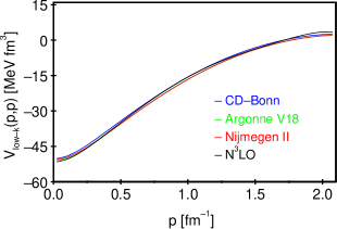
Fig. 23: (Color online) As in Fig. 22, but for the respective $V_{\rm low-k}$’s with a cutoff momentum $\Lambda=2.1$ fm^-1.

It is worth to point out that when the short-range repulsion of different $V_{NN}$’s is renormalized by means of the $G$-matrix approach the differences between these potentials are strongly quenched too. This is illustrated in Fig. 24. There we report the correlation plot between Nijmegen II and CD-Bonn matrix elements in the HO basis with the oscillator parameter $\hbar\omega=14$ MeV as well the correlation plot between the corresponding $G_{T}$ matrix elements with a Pauli operator tailored for the $sd$ shell (see Sec. 4.1.2) and a starting energy of -5 MeV. We see that while the bare matrix elements are quite different this is not the case for the $G_{T}$ matrix ones.

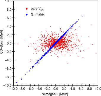
Fig. 24: (Color online) Correlation plots between Nijmegen II and CD-Bonn matrix elements and between the corresponding $G_{T}$ matrix elements (see text for details). The red and blue dots correspond to bare $V_{NN}$ and $G_{T}$-matrix elements, respectively.

Before closing this section, a brief discussion of $V_{\rm low-k}$ in the framework of the RG-EFT approach may be in order. A main point of the RG-EFT approach is that low-energy physics is not sensitive to fields beyond a cutoff scale $\Lambda$. Thus for treating low-energy physics, one just integrates out the fields beyond $\Lambda$, thereby obtaining a low-energy effective field theory. In RG-EFT, this integration out, or decimation, generates an infinite series of counter terms [158] which is a simple power series in momentum

The question as to wether the decimation of high-momentum modes in the derivation of $V_{\rm low-k}$ generates a series of counter terms has been recently investigated in Refs. [164] and [165]. In these studies it is assumed that $V_{\rm low-k}$ can be expressed as

$$V_{\rm low-k}(q,q^{\prime})\simeq V_{NN}(q,q^{\prime})+V_{\rm counter}(q,q^{\prime});~{}(q,q^{\prime})\leq\Lambda~{}~{},$$ (139)

where the counter potential is given as a power series

$$V_{\rm counter}(q,q^{\prime})=C_{0}+C_{2}q^{2}+C_{2}^{\prime}q^{\prime 2}+C_{4}(q^{4}+q^{\prime 4})+C_{4}^{\prime}q^{2}q^{\prime 2}+C_{6}(q^{6}+q^{\prime 6})+C_{6}^{\prime}q^{4}q^{\prime 2}+C^{\prime\prime}_{6}q^{2}q^{\prime 4}+~{}...$$ (140)

The counter term coefficients are determined using standard fitting techniques so that the right hand side of Eq. (139) provides a best fit to the left-hand side of the same equation. In Ref. [164] this fitting was performed over all partial wave channels and a consistently good agreement was obtained.

An examination of the counter terms was made in [164, 165], where the coefficients of some of them are also listed. A main result is that the counter terms are all rather small except for $C_{0}$ and $C_{2}$ of the $S$ waves. This is consistent with the RG-EFT approach where the counter term potential is given as a delta function plus its derivatives [158].

5 Realistic shell-model calculations

5.1 The early period

As discussed in the Introduction, while the first attempts to derive the shell-model effective interaction from the free $NN$ potential go back to some forty years ago, the practical value of this approach has emerged only during the last decade or so. On this basis, we may call the “early period” that extending over the previous three decades. It is the aim of this section to give a brief survey of the main efforts and developments made in the field during this long period of time.

The first attempt to perform a realistic shell-model calculation may be considered the one by Dawson, Talmi and Walecka [17]. They chose ¹⁸O as testing ground and approximately solved a Bethe-Goldstone equation for the wave function of the two valence neutrons using the free $NN$ potential of Brueckner-Gammel-Thaler [142] which contains a hard core. This initial approach, in which the effective interaction was simply taken to be the Brueckner reaction matrix, was followed by several authors [166, 167, 168, 169]. In this context, the merit of the various methods used to obtain the nuclear reaction matrix elements was a matter of discussion [170, 171, 172, 173].

A quantitative estimate of the core polarization effects was first given by Bertsch [174], who found, for the Kallio-Kolltveit force [168], that they can produce a correction to the interaction of two valence nucleons in ¹⁸O and ⁴²Sc as large as 30% of the $G$-matrix interaction. Soon afterwards a turning point in the development of the field was marked by the work of Kuo and Brown [18], who derived an $sd$-shell effective interaction from the Hamada-Johnston potential [63]. After having carefully evaluated the reaction matrix elements for this potential, they took into account the corrections arising from the one-particle-one-hole ($1p-1h$) excitation of the ¹⁶O core (the so-called “bubble diagram” $G_{\rm 1p1h}$). Comparison of the calculated and experimental spectra of ¹⁸O and ¹⁹F provided clear evidence of the crucial role played by the core polarization.

This remarkable achievement prompted the derivation of effective interactions for nuclei in other mass regions, such as the calcium [175], nickel [176, 177] and lead region [178, 179, 180]. These effective interactions were all deduced from the Hamada-Johnston potential by use of the $G$-matrix theory and including core-polarization effects. In this context, the individual effects of the various second-order diagrams were studied [181, 175] and the conclusion was reached that the inclusion of the core polarization diagram, $G_{\rm 1p1h}$, is generally sufficient to obtain a satisfactory agreement between calculated and experimental spectra [182].

The substantial soundness of the effective interactions derived along the lines of the Kuo-Brown approach is evidenced by the fact that, with empirical modifications, they have been used in a number of successful shell-model calculations to date. This has brought about various “semi-realistic” versions of the original Kuo-Brown interaction. In this connection, it is worth pointing out that these empirical modifications concern essentially the monopole parts of the effective interaction, as described in detail in Ref. [183], where the KB1, KB2, and KB3 interactions were introduced and applied to the study of $fp$-shell nuclei. This kind of approach, which is still favored by several authors, especially in the context of large scale shell model calculations, is outside the scope of the present article. We only mention here that recently three-body monopole corrections to realistic forces have been considered as a simple way to avoid a full treatment of three-body forces [184]. For a detailed discussion of the various effective interactions and the results of several applications, the reader is referred to the review papers by Brown [46], Otsuka et al. [48], Talmi [5], and Caurier et al. [47], where a full list of references can also be found.

It is interesting to note that in spite of the very encouraging results produced by the first generation of realistic shell-model calculations, the general attitude of the workers in the field was rather pessimistic. This is well reflected in the final statements made by Kirson in his Summary talk [185] at the 1975 Tucson International Conference:

“To summarize my summary, I would say that there are definitely major obstacles in the way of doing really convincing calculations. We have a theory, we are aware of the weakness of our computations, and we should certainly invest the effort needed to plug the more obvious holes. But we should recognize the lack of precision inherent in our inability to go to high orders in perturbation theory and adopt more qualitative methods of extracting information and gaining understanding. New ideas, new viewpoints are much needed. We should also try to withstand the temptations of seductive ¹⁸O, and pay some attention to other systems.”

The aim of the Tucson Conference [186] was to define the current status of effective interaction and operator theory in the mid 1975s. The main issues of this Conference were expounded in the subsequent excellent review by Ellis and Osnes [126]. As it emerges from the first three talks [187, 188, 189] presented at the Tucson Conference and as mentioned in Sec. 3, in the years around 1970 the theoretical bases for an energy-independent derivation of the effective interaction were laid down within the framework of the time-independent [117] as well as time-dependent [120, 121] perturbation theory. At the same time, the problems inherent in the practical application of the theory became a matter of discussion. In this context, considerable effort was made to study the convergence properties of the perturbative approach to the derivation of the effective interaction. As representative examples for these studies, we may mention here the works of Refs. [190, 191, 192, 193]. In the first of these works all significant terms through third order and a few selected fourth-order terms in the $G$ matrix were calculated and the convergence order-by-order of the perturbation series was investigated, while in the second one the focus was on the convergence rate of the sum over intermediate-particle states in the second-order core polarization contribution to the effective shell-model interaction. In the third work the authors raised the problem of the divergence of the perturbation series due to the occurrence of the so-called “intruder states”.

A most important turn in the field of realistic shell-model calculations resulted from the explicit inclusion [194, 123] of the folded diagrams in the derivation of the effective interaction within the framework of the Kuo, Lee, and Ratcliff theory [121]. In these works, starting from a realistic $G$ matrix, effective interactions for $sd$-shell nuclei were derived by means of the folded-diagram expansion, and employed in calculations for $A=18$ to 24. Note that in Ref. [123] the very convenient method proposed in [130] (see Sec. 3.3) was used to sum up the folded diagram series. It turned out that the contribution of the folded diagrams to the effective interaction is quite large, typically about 30%. In the earlier study [194] the $G$ matrix was obtained starting from the Reid soft core potential while in the later study [123] both this potential and the Paris potential were used. It may be worth noting that this latter paper was the first one where the Paris potential was employed in a microscopic calculation of finite open-shell nuclei.

As pointed out in Sec. 2.1, the advent of advanced meson-theoretic $NN$ potentials, such as the Paris and Bonn ones, was instrumental in reviving the interest in the realistic effective interactions during the 1980s. In this context, a main issue was the sensitivity of nuclear structure calculations to the strength of the tensor-force component contained in the $NN$ potential, for which a practical measure is the predicted $D$-state probability of the deuteron $P_{D}$ (see Sec. 2.1).

Earlier work on this problem was done by Sommermann et al [195] who reexamined the intermediate state convergence problem for the core polarization diagram in the expansion of an effective shell-model interaction using the Bonn-Jülich (MDFP$\Delta$2) potential [196, 197] in comparison to the Reid soft-core interaction [64]. It is a remarkable achievement of this work to have shown that the so-called Vary-Sauer-Wong effect, namely the slow rate of convergence found for the Reid potential [191, 198], was of negligible importance for the Bonn-Jülich potential, as a consequence of the much weaker tensor force contained in the latter.

Some ten years later, using a $G$-matrix folded-diagram method, the $sd$-shell effective interaction was derived from various potentials and applied to calculate the spectra of some light $sd$-shell nuclei [199]. In particular, the three variants of the OBE parametrization of the Bonn full model, Bonn A, Bonn B, and Bonn C, differing in the strength of the tensor force (see Sec. 2.1) as well as the Paris potential, were considered. It turned out that the best agreement with experiment was achieved with the weakest tensor force potential (Bonn A).

The development of more realistic $NN$ potentials, such as the Bonn and Paris potentials, led also in the early 1990s to new studies of the role of the third- and higher-order perturbative contributions to the effective interaction, which had been investigated some twenty years before in the work of Ref. [190]. Within the framework of the folded diagram theory, the inclusion of the third-order diagrams in $G$ in the calculation of the $\hat{Q}$-box was studied and the order-by-order convergence of the effective interaction in terms of the mass number $A$ was examined [200, 201, 202, 203]. The main findings of the last study of this series [203] were that the convergence of the perturbation expansion seems to be rather insensitive to the mass number and that the effects of third-order contributions in the $T=1$ channel are almost negligible. We refer to Ref. [45] for a review of the status of the theory of realistic effective interactions in the mid 1990s.

We have given above a brief review of the great deal of work done in the field of realistic shell-model calculations during what we have called, somewhat arbitrarily, the “early period”. Before finishing this subsection, a word is in order concerning this choice of presentation, which, in our opinion, reflects how hard it has been to make this kind of calculations a reliable tool for quantitative nuclear structure studies.

We draw the reader’s attention to the fact that, after the calculations performed by Kuo and collaborators from the mid 1960’s up to the mid 1970’s [175, 176, 177, 178, 179, 180], practically no other calculations were done for about two decades having as only aim a detailed description of nuclear structure properties. This lack of confidence in the predictive power of realistic effective interactions is well evidenced by the fact that in almost all the papers on this subject published from the mid 1970’s up to about the early 1990’s, the focus has been on nuclei of the $sd$-shell, considered as a necessary testing ground for the effective interaction before embarking on a more ambitious program of applications. In this connection, the warning by Kirson (see above citation) against the temptations of seductive ¹⁸O acquires a particular significance.

5.2 Modern calculations

As discussed in the previous subsection, during the 1980s a substantial progress was made in the practical application of shell model with realistic effective interactions. This has resulted in a new generation of realistic shell-model calculations oriented to the study of the spectroscopic properties of nuclei in various mass regions.

The first attempts in this direction focused on the Sn isotopes [204, 45, 205], in particular on the neutron deficient ones. In the work of Ref. [204] the Bonn A potential was used while in that of Ref.  [45] results obtained with the stronger tensor-force versions of this potential (Bonn B and Bonn C) were also reported. In both these works all two-body diagrams through third order in the $G$ matrix were included in the $\hat{Q}$-box. In the study of Andreozzi et al. [205] both the Paris and Bonn A potentials were employed and the $\hat{Q}$-box was taken to be composed of diagrams through second order in $G$ (a comparative discussion of the above studies can be found in [205]). The results of these initial “modern” calculations, in particular those obtained with the Bonn A potential, turned out to be in remarkably good agreement with the experimental data.

These achievements encouraged further work along these lines. In the few following years realistic shell-model calculations were carried out for a number of nuclei around doubly magic ¹⁰⁰Sn [134], ¹³²Sn [206, 207, 208, 209], and ²⁰⁸Pb [210, 211, 212]. Note that in all these calculations, except the one of Ref. [209] where the CD-Bonn 1996 potential [87] was employed, the effective interaction was derived from the Bonn A potential. We refer to Covello et al. [39] for a survey of the status of realistic shell-model calculations at the end of the 1990s. Suffice it to say here that the rms deviation for the spectra of 15 medium- and heavy-mass nuclei reported in this paper is in 7 cases less than 100 keV, only in one case reaching 165 keV.

The success achieved by these calculations gave a clear-cut answer to the crucial, long-standing problem of how accurate a description of nuclear structure properties can be provided by realistic effective interactions, opening finally the way to a more fundamental approach to the nuclear shell model than the traditional, empirical one.

As is well known, much attention is currently being focused on nuclei in the regions of shell closures off stability, as they allow to explore for possible shell-structure modifications when approaching the proton and neutron drip lines. The experimental study of these nuclei is very difficult, but in recent years new data have become available for some of them, which provide a challenging testing ground for realistic effective interactions. Starting in the early 2000s, several “exotic” nuclei around doubly magic ¹⁰⁰Sn and ¹³²Sn have been studied employing realistic effective interactions derived from the high-precision CD-Bonn $NN$ potential [88]. In the first paper of this series [213] shell-model calculations were performed for Sn isotopes beyond $N=82$, in particular the heaviest Sn isotope known to date, ¹³⁴Sn. In this work, similarly to what had been done in their previous papers, the authors employed a $G$-matrix folded-diagram formalism. A very good agreement was found between the calculated results and the available experimental data.

A most important turn in the derivation of the effective interaction from the free $NN$ potential has resulted from the development of the $V_{\rm low-k}$ approach (see Sec. 4.2). This approach to renormalize the short-range repulsion of $V_{NN}$ has been recently used in several calculations. Attention has been focused on exotic nuclei neighboring ¹⁰⁰Sn [214], and ¹³²Sn [215, 216, 217, 163, 218, 219]. Actually, most of these works are concerned with nuclei in the latter region, for which there are new interesting experimental data. The agreement between theory and experiment has turned out to be very good in all cases. This supports confidence in the predictions of these realistic calculations, which may therefore stimulate and be helpful to, future experiments. To illustrate this important point, we shall review in Sec. 5.3.3 some selected results for ¹³²Sn neighbors with neutrons beyond the 82 shell.

While most of the realistic shell-model calculations carried out in last few years have employed effective interactions derived from the CD-Bonn $NN$ potential, some attempts to put to the test chiral potentials have also been made. Representative examples for these studies are the works of Refs. [220, 221, 222, 223], all of them making use of the $V_{\rm low-k}$ renormalization method. Actually, only in [220], where the NNLO Idaho potential [104] was used, shell model calculations for various two valence-particle nuclei were performed. In the other three works [221, 222, 223] ground-state properties of doubly magic nuclei ⁴He, ¹⁶O, and ⁴⁰Ca were calculated within the framework of the Goldstone expansion [122] with the N³LO potential [102]. The results obtained in [220] turned out to be comparable to those produced by effective interactions derived from the CD-Bonn potential. Clearly, this is related to the important question of how much nuclear structure results depend on the $NN$ potential one starts with. We shall discuss this point in Sec. 5.3.2.

5.3 Results

5.3.1 Comparison between $G$-matrix and $V_{\rm low-k}$ approaches

As evidenced by the discussion given in Secs. 5.1 and 5.2, for about forty years the Brueckner $G$ matrix represented practically the only tool to renormalize the repulsive core contained in the $NN$ potential. After its introduction, the $V_{\rm low-k}$ potential has been readily seen as an alternative to the $G$ matrix. In fact, $V_{\rm low-k}$ is a smooth free-space potential and its matrix elements between unperturbed two-particle states can be directly used as input to the $\hat{Q}$-box folded-diagram procedure of Sec. 3. Therefore, a main issue has been to assess the merit of the $V_{\rm low-k}$ approach in practical applications.

First work along this line was done by Kuo et al. [224], who carried out shell-model calculations for ¹⁸O using two-body matrix elements of effective interactions derived from the Bonn A and Paris potentials. Other studies [225, 43, 226] were then performed which, starting from the CD-Bonn potential, extended the comparison between the $G$ matrix and $V_{\rm low-k}$ approaches to nuclei heavier than ¹⁸O. In particular, the calculations of Ref. [225] concern ¹³²Sn neighbors, while results for ¹⁸O, ¹³⁴Te, and ¹³⁵I are presented in [43]. A comparison between the $G$ matrix and $V_{\rm low-k}$ spectra for the heavy-mass nucleus ²¹⁰Po can be found in [226]. In all these calculations the cutoff parameter $\Lambda$ is chosen in the vicinity of 2 fm^-1.

It has been a remarkable finding of all these studies that the $V_{\rm low-k}$ results are as good or even slightly better than the $G$-matrix ones. The rather close similarity between the results of the two approaches finds an exception for the Paris potential [224]. We shall comment on this point in Sec. 5.3.2. It is also important to point out that the $V_{\rm low-k}$ approach appears to work equally well in different mass regions. A detailed description of the above mentioned calculations can be found in the cited references. Here, for the sake of completeness, we report two examples concerning ¹⁸O and ¹³⁴Te, which are both taken from [43], where more details about the calculations can be found.

The experimental and calculated spectra of ¹⁸O including the five lowest-lying states, and those of ¹³⁴Te with the eight lowest-lying states are reported in Figs. 25 and 26, respectively. The calculated spectra have been obtained from the CD-Bonn potential through both the $V_{\rm low-k}$ and $G$-matrix folded-diagram approaches. As for the $V_{\rm low-k}$ calculations, two values of the cutoff momentum have been used, $\Lambda=2.0$ and 2.2 fm^-1. For ¹⁸O we have adopted a model space with the two valence neutrons in the $(0d_{5/2},0d_{3/2},1s_{1/2})$ shell, while for ¹³⁴Te the two valence protons are allowed to occupy the levels of the $(0g_{7/2},1d_{5/2},1d_{3/2},2s_{1/2},0h_{11/2})$ shell. In both cases the SP energies are taken from experiment, in particular from the spectra of ¹⁷O and ¹³³Sb for the $sd$ and $sdgh$ shells, respectively. The energy of the $2s_{1/2}$ proton level, which is still missing, is from the study by Andreozzi et al. [206]. Note that in Figs. 25 and 26 the energies are relative to the ground state of the neighboring doubly closed nucleus ¹⁶O and ¹³²Sn, respectively, with the mass-excess values for ¹⁷O and ¹³³Sb needed for the absolute scaling of the SP energies coming from Refs. [227] and [228]. As for ¹³⁴Te, the Coulomb contribution was taken into account by adding to the CD-Bonn effective interaction the matrix element of the Coulomb force between two $g_{\frac{7}{2}}$ protons with $J=0$.

Fig. 25: Low-lying states in ¹⁸O.

As pointed out above, we see from Figs. 25 and 26 that the $V_{\rm low-k}$ and $G$-matrix results are rather close to each other and in quite good agreement with experiment. It is worth noting that the $V_{\rm low-k}$ results for the two values of $\Lambda$ do not differ significantly. We shall come back to this point later.

In this context, we may also mention the work of Refs. [229] and [230], where harmonic-oscillator matrix elements of the $V_{\rm low-k}$ potential and $G$ matrix are compared in 4 major shells. It was found that both the $T=0$ and $T=1$ matrix elements are very similar.

On the above grounds, the conclusion is reached that the $V_{\rm low-k}$ approach is a reliable way to renormalize the bare $NN$ potential before employing it in the derivation of the shell-model effective interaction.

Another relevant point to be stressed is that the $V_{\rm low-k}$ is far easier to be used than the $G$ matrix. In fact, $V_{\rm low-k}$ is a soft $NN$ potential and as such does not depend either on the starting energy or on the model space, as is instead the case of the $G$ matrix, which is defined in the nuclear medium. This has the desirable consequence that the $V_{\rm low-k}$ matrix element to be used in an interaction vertex of a given $\hat{Q}$ box diagram is completely determined by the incoming and outcoming lines attached to the vertex under consideration. Hence, it does not depend on any other part of the diagram. Also, it is worth noting that the same $V_{\rm low-k}$ can be used in different mass regions.

Finally, when considering the features of the $V_{\rm low-k}$ approach, one has also to keep in mind that, as discussed in Sec. 4.2.3, different $NN$ potentials lead to low-momentum potentials which are remarkably similar to each other. In the same section, we have showed that the differences between the different potentials are also quenched within the $G$ matrix approach. This will be further discussed in Sec. 5.3.2.

We conclude by mentioning that the $V_{\rm low-k}$ approach has also proved to be an advantageous alternative to the $G$ matrix in the calculation of the ground-state properties of doubly closed nuclei. As is well known, the traditional approach to this problem is the Brueckner-Hartree-Fock (BHF) theory. In the study of Ref. [221] it has been showed that the $V_{\rm low-k}$ is suitable for being used directly in the Goldstone expansion. Good results for ¹⁶O and ⁴⁰Ca were obtained by solving the Hartree-Fock (HF) equations for $V_{\rm low-k}$ and then using the resulting self-consistent basis to compute higher-order Goldstone diagrams. In this connection, it should be mentioned also the work of Ref. [231], where use was made of the $V_{\rm low-k}$ potential in a HF and BHF approach to evaluate the binding energy and the saturation density of nuclear matter and finite nuclei. Their conclusion was that for nuclear matter at small and medium densities as well as for finite nuclei HF and BHF results with $V_{\rm low-k}$ are nearly identical.

Fig. 26: Low-lying states in ¹³⁴Te.

5.3.2 Calculations with different $NN$ potentials

As discussed in Sec. 5, a main problem relevant to realistic shell-model calculations has been to assess the accuracy of the effective interaction derived from the $NN$ potential. However, it is also an important issue what information comes out on the $NN$ potential from this kind of calculations. As we have seen in Sec. 2, from the early 1950s on several different potentials have been constructed. The potentials of the last generation all fit equally well the $NN$ phase shifts, but, except for the OPE tail, they are quite different from each other. Actually, these potentials are well-constrained by the deuteron properties and the $NN$ scattering data for $E_{\rm lab}<350$ MeV and therefore their offshell behavior is subject to ambiguities. This is reflected in the different values predicted for the $D$-state probability of the deuteron $P_{D}$ (see Sec. 2) as well as in the different binding energies calculated for $A=3,4$ systems [232]. In fact, for $A>2$ the interaction may be off the energy shell since two nucleons may have different energies before and after they interact.

In this context, it is of great interest to perform nuclear structure calculations to see to which extent the differences between $NN$ potentials persist once the short-range repulsion is renormalized through the $G$-matrix or the $V_{\rm low-k}$ approach. This problem has long been investigated by studying properties of both nuclear matter and doubly closed nuclei. A list of references on this subject can be found in the work of Ref. [222], which we have briefly discussed in Secs. 4.2.3 and 5.2. As for open-shell nuclei, some attempts have been made within the framework of the shell model.

In the early work by Sommermann et al. [195], the comparison between Bonn-Jülich and Reid results aimed at investigating the intermediate-state convergence problem, as discussed in Sec. 5.1. The paper by Shurpin et al. [123] had instead as a main purpose to compare the spectra of several $sd$-shell nuclei calculated with two different potentials, Paris and Reid. The results showed that the Paris potential was as good as, if not better than, the Reid potential. The idea of comparing shell-model calculations with different $NN$ potentials was revived at the end of the 1980s. In the works of Refs. [233, 199] and [234] $sd$-shell nuclei were studied using as input several different $NN$ potentials, all constructed before the 1990s. These works were based on the use of the reaction matrix $G$ to derive the effective interaction through the $\hat{Q}$-box folded-diagram method, including up to second-order diagrams. The outcome of these studies was that the effective interaction matrix elements become more attractive when a $NN$ potential with a weaker tensor-force strength is used. Jiang et al. [199] noted that the nonlocality of the potential gives a further contribution in this direction. All these calculations indicated in general that the best agreement with experiment was produced by the Bonn potential.

A confirmation of the important role played by weaker tensor force potentials came out from the paper of Ref. [205], where Paris and Bonn A results for neutron deficient Sn isotopes are compared. A better agreement with experiment was obtained with the Bonn A potential. The merit of potentials with weak tensor force was also evidenced in [45], who performed realistic shell-model calculations for nuclei in the mass regions of ¹⁶O, ⁴⁰Ca, and ¹⁰⁰Sn using the three variants (A, B, and C) of the Bonn potential.

A comparative study of shell-model results obtained from different $NN$ potentials, including the high-precision CD-Bonn potential, was made for the first time in [235]. In this paper, the nucleus ¹³⁴Te was used as a testing ground to investigate the effects of the CD-Bonn potential with respect to those of the three potentials Bonn A, Paris, and Nijm93. As in all previous calculations, it was found that a weak tensor force leads to a better description of nuclear structure properties. Furthermore, it turned out that the calculated spectra, except that obtained from the Paris potential, are only slightly different from each other.

Fig. 27: Spectrum of ¹³⁴Te. Predictions by various $NN$ potentials are compared with experiment.

All the above calculations made use of the reaction matrix $G$ and their results provide evidence that the differences existing between various potentials are quenched by the $G$-matrix renormalization procedure (see Fig. 24). One may wonder what happens when the $V_{\rm low-k}$ potential is used. The first answer to this question may be found in [224], where the $V_{\rm low-k}$ approach is used to calculate the Paris and Bonn A spectra for ¹⁸O. It is interesting to note that these two spectra are much closer to each other than those obtained with the $G$ matrix approach [199]. This reflects the fact that the $V_{\rm low-k}$ procedure is more effective in reducing the differences between the two potentials than the $G$-matrix approach. The matrix elements in the ${}^{3}S_{1}$ channel for both Paris and Bonn A potentials are reported in Fig. 1 of [224], where it is shown that they become similar after the $V_{\rm low-k}$ renormalization, the latter being much larger for the strongly repulsive Paris potential.

In Sec. 4.2.3 (see Figs. 22 and 23), we have reported a similar comparison in the ${}^{1}S_{0}$ channel for the chiral potential N³LO and the three high-precision potentials CD-Bonn, NijmII, and Argonne $V_{18}$. The differences between the matrix elements of these potentials practically disappear when the $V_{\rm low-k}$ matrix elements are considered. On these grounds one expects that shell-model effective interactions derived from phase-shift equivalent $NN$ potentials through the $V_{\rm low-k}$ approach should lead to very similar results.

This we have verified by calculating the spectra of ¹³⁴Te starting from the CD-Bonn, NijmII, and Argonne $V_{18}$ potentials. For all the three $V_{\rm low-k}$’s derived from these $NN$ potentials, use has been made of the same cutoff momentum $\Lambda=2.2$ fm^-1. Other details on how these calculations have been performed may be found in Sec. 5.3.3, where we present results for nuclei beyond ¹³²Sn, which have been obtained using the CD-Bonn potential.

In Fig. 27, the three calculated spectra are shown and compared with the experimental one. Note that, with respect to Fig. 26, the energies are relative to the ground state and higher lying levels are included. We see that the calculated spectra are very similar, the differences between the predicted energies not exceeding 80 keV. It is also seen that the agreement with experiment is very good for all the three potentials. In fact, the rms deviation is 115, 128, and 143 keV for CD-Bonn, Argonne $V_{18}$, and NijmII, respectively.

Finally, it is of interest to make a few comments regarding the value of the cutoff momentum $\Lambda$. In Sec. 4.2.3 the plausibility of using a value in the vicinity of 2 fm^-1 was discussed. It was also shown in Sec. 5.3.1 that shell-model results do not change significantly when varying $\Lambda$ from 2 to 2.2 fm^-1. A preliminary study of the dependence of shell-model results on $\Lambda$ can be found in the work of Ref. [236], where results for ¹³⁴Te are reported using the CD-Bonn, Argonne $V_{18}$, and NijmII potentials with $\Lambda$ varying over a rather large range (1.5-2.5 fm^-1). It has been found that the best agreement with experiment for each of these three potentials corresponds to a somewhat different value of $\Lambda$. However, changes around this value do not significantly modify the quality of agreement for all the three potentials. As an example, the rms deviation for NijmII remains below 150 keV for any value of $\Lambda$ between 1.8 and 2.2 fm^-1 This subject deserves certainly further studies.

5.3.3 Neutron rich nuclei beyond ¹³²Sn: comparing theory and experiment

The study of exotic nuclei is a subject of a current experimental and theoretical interest. Experimental information for nuclei in the vicinity of ⁷⁸Ni, ¹⁰⁰Sn, ¹³²Sn, which have been long inaccessible to spectroscopic studies, is now available thanks to new advanced facilities and techniques. The advent of radioactive ion beams is opening new perspectives in this kind of studies. Nuclei in the regions of shell closures are a source of direct information on shell structure. New data offer therefore the opportunity to test the shell model and look for a possible evolution of shell structure when going toward proton or neutron drip lines.

This is stimulating shell-model studies in these regions. Several realistic shell-model calculations have been recently performed for nuclei around ¹⁰⁰Sn and ¹³²Sn, as mentioned in Sec. 5.2. We report here some selected results on ¹³²Sn neighbors with $N>82$. More precisely, we consider the three nuclei ¹³⁴Sn, ¹³⁴Sb, and ¹³⁵Sb, which have been very recently studied in [219], [218], and [163], to which we refer for a more detailed discusssion.

Fig. 28: Experimental and calculated spectra of ¹³⁴Sn.

The experimental data which have been now become available for these neutron-rich nuclei may suggest a modification in the shell structure. They are, in fact, somewhat different from what one might expect by extrapolating the existing results for $N<82$, and as a possible explanation a change in the single-proton level scheme has been suggested. The latter, caused by a more diffuse nuclear surface, may be seen as a precursor of major effects which should show up at larger neutron excess.

We shall see now that the properties of these three nuclei are all well accounted for by a shell-model calculation with a two-body effective interaction derived from a modern $NN$ potential. In so doing, we evidence the merit of realistic shell-model calculations, showing, at the same time, that there is no need to invoke new effects to describe few-valence-particle nuclei just above ¹³²Sn. In this connection, it is worth mentioning that different shell-model calculations have been performed for the above nuclei [237, 238, 239, 240, 241, 242]. None of these studies, however, has succeeded in accounting simultaneously for the peculiar features of all the three nuclei.

Fig. 29: Experimental and calculated spectra of ¹³⁴Sb.

In our calculations, we assume that ¹³²Sn is a closed core and let the valence neutrons occupy the six levels $0h_{9/2}$, $1f_{7/2}$, $1f_{5/2}$, $2p_{3/2}$, $2p_{1/2}$, and $0i_{13/2}$ of the 82-126 shell, while for the proton the model space includes the five levels $0g_{7/2}$, $1d_{5/2}$, $1d_{3/2}$, $2s_{1/2}$, and $0h_{11/2}$ of the 50-82 shell. The proton and neutron single-particle energies have been taken from the experimental spectra of ¹³³Sb and ¹³³Sn, respectively, the only exceptions being those of the $s_{1/2}$ proton and $i_{13/2}$ neutron levels which are still missing. The energy of the former, as mentioned in Sec. 5.3.1, is from [206], while that of the latter from [213]. The two-body matrix elements of the effective interaction have been derived from the CD-Bonn $NN$ potential. This potential is renormalized by constructing the $V_{\rm low-k}$ with a cutoff momentum $\Lambda$ =2.2 fm^-1. The effective interaction has been then derived within the framework of the $\hat{Q}$-box plus folded diagram method including diagrams up to second order in $V_{\rm low-k}$. The computation of these diagrams is performed within the harmonic-oscillator basis using intermediate states composed of all possible hole states and particle states restricted to the five shells above the Fermi surface. This guarantees the stability of the results when increasing the number of intermediate particle states. The oscillator parameter used is $\hbar\omega=7.88$ MeV and for protons the Coulomb force has been explicitly added to the $V_{\rm low-k}$ potential.

Fig. 30: Experimental and calculated spectra of ¹³⁵Sb.

The experimental and calculated spectra of ¹³⁴Sn, ¹³⁴Sb, and ¹³⁵Sb are compared in Figs. 28, 29, and 30, respectively. Note that both the calculated and experimental spectra of ¹³⁴Sb include all levels lying below 1 MeV excitation energy, while for ¹³⁵Sb all the yrast states have been reported. As for ¹³⁴Sn, only the levels reported in Fig. 28 have been observed, while in the calculated spectrum five states, predicted in between the $6^{+}$ and $8^{+}$ states, are omitted.

The two isotones with $A=134$ are the most appropriate systems to study the effects of the effective interaction. In fact, ¹³⁴Sn is a direct source of information on the neutron-neutron channel while ¹³⁴Sb on the proton-neutron one. The nucleus ¹³⁵Sb represents a further interesting test, since it allows to investigate at once the role of the effective interaction in both channels.

From the above figures, we see that the experimental levels in all the three nuclei are very well reproduced by the theory, the discrepancies being of the order of few tens of keV for most of the states. Note that the very low-energy positions of both the first-excited $2^{+}$ and $1^{-}$ states in ¹³⁴Sn and ¹³⁴Sb, respectively, are well accounted for, as is also the case for the low excitation energy of the $5/2^{+}$ state in ¹³⁵Sb. We refer to the above mentioned papers for more details on each of the three calculations and for a discussion of the structure of the states in ¹³⁴Sb and ¹³⁵Sb. As for the latter, it is shown in [163] that it is the admixed nature of the $5/2^{+}$ state that explains its anomalously low position and the strongly hindered $M1$ transition to the ground state. The role of the effective interaction as well as of the $5/2^{+}$ single-proton energy in determining this situation has been examined, with particular attention to the effects induced by the proton-neutron interaction. The relevant role of the latter was also evidenced in ¹³⁴Sb [218]. For this nucleus, a direct relation can be established between the diagonal matrix elements of the proton-neutron effective interaction and the calculated energies reported in Fig. 29, since the corresponding wave functions are characterized by very little configuration mixing. In particular, the eight lowest-lying states can be identified with the eight members of the $\pi g_{7/2}\nu f_{7/2}$ multiplet while the two higher states, with $J^{\pi}=1^{-}$ and $2^{-}$, are the only members of $\pi d_{5/2}\nu f_{7/2}$ multiplet having an experimental counterpart.

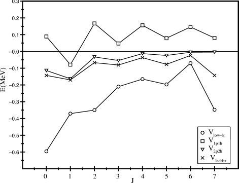
Fig. 31: Diagonal matrix elements of the $V_{\rm low-k}$ and contributions from the two-body second-order diagrams for the $\pi g_{7/2}\nu f_{7/2}$ configuration.

In this connection, it may be interesting to summarize here the analysis of the proton-neutron matrix elements reported in the work of Ref. [218]. Focusing on the $\pi g_{7/2}\nu f_{7/2}$ configuration, we examine the various terms which contribute to the effective interaction, namely the $V_{\rm low-k}$ and all the second-order two-body diagrams composing the $\hat{Q}$ box. It is worth pointing out that the effective interaction $V_{\rm eff}$ is obtained by summing to the $\hat{Q}$-box the folded-diagram series [see Eq. (58)], but the contribution of the latter provides a common attenuation for all matrix elements, thus not affecting the following discussion.

The diagonal matrix elements of $V_{\rm low-k}$ for the $\pi g_{7/2}\nu f_{7/2}$ configuration are reported in Fig. 31 as a function of $J$ together with the contributions arising from the $1p-1h$, $2p-2h$, and ladder excitations. In Fig. 32 we present for the same configuration the diagonal matrix elements of the effective interaction which we have obtained starting from this $V_{\rm low-k}$. Note that the behavior of $V_{\rm eff}$ shown in Fig. 32 is quite similar to that of the $\pi g_{7/2}\nu f_{7/2}$ multiplet in ¹³⁴Sb, whose members, as mentioned above, are almost pure. This behavior, however, is quite different from that of $V_{\rm low-k}$, especially as regards the $0^{-}-1^{-}$ spacing. This means that the second-order two-body contributions accounting for configurations left out of the chosen model space are of key importance to renormalize the $V_{\rm low-k}$ and get the correct behavior. In particular, a crucial role is played by the core-polarization effects arising from the $1p-1h$ excitations.

At this point one may wonder why our effective interaction is able to explain the properties of these neutron-rich nuclei above ¹³²Sn while the realistic shell-model calculations of Refs. [237, 238, 239] do not. In the latter calculations the effective interaction has been derived within the $G$-matrix folded-diagram approach including in the $\hat{Q}$-box diagrams up to third order in $G$ and intermediate states with at most $2\hbar\omega$ excitation energy [203]. With this interaction, a satisfactory agreement with experiment was obtained only for ¹³⁴Sn when using experimental SP energies. A downshift of the $\pi d_{5/2}$ level with respect to the $\pi g_{7/2}$ one by 300 keV turned out to be necessary to obtain a good description of ¹³⁵Sb [237, 239], but did not help for ¹³⁴Sb [238]. We have verified that the differences between the results presented in this section and those of Refs. [237, 238, 239] can be traced mainly to the different dimension of the intermediate state space. In fact, we have found that including intermediate states only up to $2\hbar\omega$ excitation energy in our derivation of the effective interaction, the results of the two calculations become very similar.

In summary, we have shown that modern realistic shell-model calculations are able to describe with quantitative accuracy the spectroscopic properties of ¹³⁴Sn, ¹³⁴Sb, and ¹³⁵Sb, in particular, their peculiar features. This leads to the conclusion that a consistent description of ¹³²Sn neighbors with neutrons beyond the $N=82$ shell is possible. In this connection, it is worth mentioning two more recent works [243, 244], where shell-model results for other nuclei around doubly magic ¹³²Sn are reported, including predictions for ¹³⁶Sn.

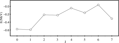
Fig. 32: Diagonal matrix elements of the two-body effective interaction for the $\pi g_{7/2}\nu f_{7/2}$ configuration.

5.3.4 The role of many-body forces

In this subsection, we shall discuss the role that the $3N$ forces, both real and effective, play in shell-model calculations based on the results we obtain for the even-mass $N=82$ isotonic chain. This study has been performed with the same input for all nuclei of the isotonic chain, namely the SP energies and the matrix elements of the two-body effective interaction employed in the calculations discussed in Sec. 5.3.3. Here, the shell-model calculations have been carried out by using the Oslo code [245].

Let us first consider the two valence-proton system ¹³⁴Te. As mentioned in Sec. 2.3, a genuine $3N$ potential, which may affect the one- and two-body components of the shell-model effective interaction $H_{\rm eff}^{1}$ of Eq. (58), has never been considered explicitly. The contributions of the $3N$ potential to the one-body term of $H_{\rm eff}^{1}$ may be assumed as taken into account when, as usual,the SP energies are taken from the experimental data. As regards the contribution of the $3N$ potential to the two-body component of $H_{\rm eff}^{1}$, it may be reduced with an appropriate choice of the cutoff momentum $\Lambda$ of the $V_{\rm low-k}$. In [229], it was suggested to choose $\Lambda$ around 2 fm^-1, since this value seems to minimize the role of the $3N$ potential when calculating the ³H and ⁴He binding energies. In this context, it is worth recalling that here we have used experimental SP energies and an effective interaction derived from a $V_{\rm low-k}$ with $\Lambda=2.2$ fm^-1.

For the ground-state energy of ¹³⁴Te, relative to the doubly magic ¹³²Sn, we obtain a value of -20.796 MeV to be compared with the experimental one -20.584 MeV. As regards the energy spectrum, the rms deviation is 0.115 MeV (see Fig. 27). These results seem to validate for many-nucleons systems the hypothesis made in [229] about the choice of $\Lambda$.

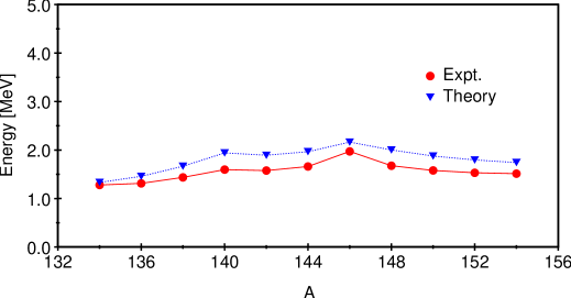
Fig. 33: Excitation energies of the $J=2^{+}$ yrast states for $N=82$ isotones as a function of mass number $A$.

Let us now come to nuclei with more than two valence nucleons. We know that in this case many-body terms appear in the shell-model effective interaction, even if the original potential is only a two-body one. The effects of these terms have not yet been quantitatively evaluated [11, 38, 246, 247]. However, it is generally believed that effective many-body forces have little influence on the excitation energies, while the binding energies may be significantly affected [127]. In this connection, it may be mentioned that Talmi [248] has shown that the experimental binding energies of the tin isotopes can be reproduced quite accurately employing an empirical two- and three-body interaction.

In order to study the effective many-body forces, we have calculated the excitation energies of the lowest-lying yrast states in the even $N=82$ isotones. In Figs. 33, 34, and 35, the calculated energy of the $J^{\pi}=2^{+}$, $4^{+}$, and $6^{+}$ states, respectively, are reported as a function of the mass number $A$ and compared with the experimental data. It is seen that the agreement between theory and experiment is of the same quality all over the isotonic chain, thus confirming that effective many-body forces play a negligible role in the description of the relative energy spectra.

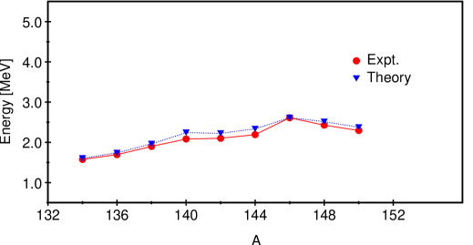
Fig. 34: Same as in Fig.33 but for $J=4^{+}$.

In Fig. 36, we report the ground-state energy per valence nucleon. It appears that the experimental and theoretical behaviors diverge when increasing the number of protons. As in the case of tin isotopes [249], the binding energy is increasingly overestimated. This deficiency may be healed by adding a small repulsive monopole contribution, whose origin may be traced to effective many-body forces [248].

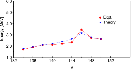
Fig. 35: Same as in Fig.33 but for $J=6^{+}$.

6 Summary and conclusions

In this paper, we have tried to give a self-contained review of the present status of shell-model calculations employing two-body effective interactions derived from the free nucleon-nucleon potential. A main feature of this kind of calculations, which are commonly referred to as realistic shell-model calculations, is that no adjustable parameter appears in the determination of the effective interaction. This removes the uncertainty inherent in the traditional use of empirical interactions.

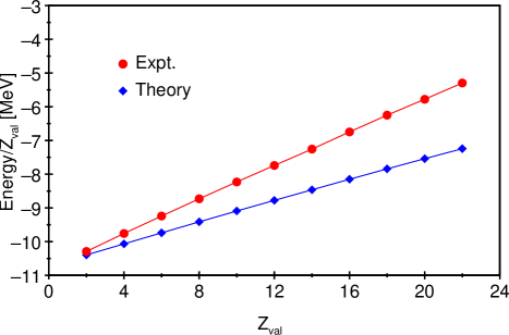
Fig. 36: Ground-state energies per valence proton of $N=82$ isotones as a function of the valence-proton number $Z$.

As discussed in the Introduction, only in the last few years has this approach, which started in the 1960s, acquired a reputation for being able to provide an accurate description of nuclear structure properties. This means that to place in its proper perspective the current status of the field it is helpful to look back and survey the difficulties faced and the progress achieved over about four decades. The present review, while aimed at giving an insight into modern realistic shell-model calculations, is also concerned with the above aspects in regard to both the $NN$ potential and the many-body methods for deriving the effective interaction.

As regards the first issue, in Sec. 2 we have discussed in some detail the main advances in the understanding of the $NN$ interaction from the early stages of development until the current efforts based on chiral effective field theory. This we have done to show how the advances in this field have been intimately related to the development of realistic nuclear structure calculations. The present stage of development is certainly enough to provide a sound starting point for a quantitative description of nuclear structure properties. It remains a main task for the near future to assess the role of the three-body forces in many-nucleon systems. A brief discussion on this matter is given in Sec. 5.3.4 based on the results for the even $N=82$ isotones.

In Sec. 3 we have described how the shell-model effective interaction can be derived within the framework of degenerate time-dependent perturbation theory.

The problem of the short-range repulsion contained in the $NN$ potential has been discussed in Sec. 4, where, after an outline of the traditional Brueckner $G$-matrix method, we have described a new approach to the renormalization of $V_{NN}$, which consists in constructing a low-momentum $NN$ potential, $V_{\rm low-k}$, that preserves the physics of $V_{NN}$ up to a cutoff momentum $\Lambda$. Since $V_{\rm low-k}$ is already a smooth potential, it can be used directly as input for the derivation of the shell-model effective interaction instead of the usual $G$ matrix. While its merit in this respect has been assessed by several calculations (Sec. 5.3.1) the $NN$ potential $V_{\rm low-k}$ is currently attracting much attention. On the one hand, it is being applied in various contexts, for instance in the study of few-body problems [250, 114]. On the other hand, its properties are being studied in detail, in particular as regards the dependence on the original potential model [251, 222, 236]. Concerning shell-model calculations, results obtained with different $NN$ potentials using the $V_{\rm low-k}$ approach have been presented in Sec. 5.3.2.

A main motivation for this review has been the practical success achieved by realistic shell-model calculations in the last few years, after a long period of hope and dismay. In Sec. 5. we have first surveyed the main efforts in this field going from the early to present days. We have then presented, by way of illustration, some selected results of recent calculations for nuclei around doubly magic ¹³²Sn. These neutron-rich nuclei, which lie well away from the valley of stability, offer the opportunity for a stringent test of the matrix elements of the effective interaction. The very good agreement with the available experimental data shown in Sec. 5.3.3 supports confidence in the predictive power of realistic shell-model calculations in the regions of shell closures off stability, which are of great current interest.

As already pointed out above, in this review our focus has been on shell-model calculations employing genuine free $NN$ potentials. As a consequence of this choice, even a brief summary of the many successful shell-model calculations employing modified versions of free $NN$ potentials would have been beyond the scope of the present article. Here, we have also not touched upon another important aspect of shell-model work, namely the development of new methods, such as the Monte Carlo shell model (MCSM), as well as of high-quality codes, such as ANTOINE [252], which has greatly extended the feasibility of large-scale calculations. However, both these issues are discussed in detail in the recent article by Caurier et al. [47] while for a specialized review of the MCSM we refer to Ref. [48].

To conclude, we may say that the stage for realistic shell-model calculations is by now well set, which is a major step towards the understanding of the properties of complex nuclei in terms of the forces among nucleons. In this context, the $V_{\rm low-k}$ approach provides a new effective tool to handle the short-range repulsion of the free $NN$ potential.

References

- [1] M.G. Mayer, Phys. Rev. 75 (1949) 1969.
- [2] O. Haxel, J.H.D. Jensen and H.E. Suess, Phys. Rev. 75 (1949) 1766.
- [3] M.G. Mayer and J.H.D. Jensen, Elementary theory of nuclear shell structure (John Wiley, New York, 1955).
- [4] M.G. Mayer, Phys. Rev. 78 (1950) 22.
- [5] I. Talmi, Adv. Nucl. Phys. 27 (2003) 1.
- [6] S.C. Pieper et al., Phys. Rev. C 64 (2001) 014001.
- [7] S.C. Pieper and R.B. Wiringa, Annu. Rev. Nucl. Part. Sci. 51 (2001) 53.
- [8] P. Navratil and B.R. Barrett, Phys. Rev. C 54 (1996) 2986.
- [9] P. Navratil, J.P. Vary and B.R. Barrett, Phys. Rev. Lett. 84 (2000) 5728.
- [10] K. Suzuki et al., Nucl. Phys. A 567 (1994) 576.
- [11] D.J. Dean et al., Prog. Part. Nucl. Phys. 53 (2004) 419.
- [12] K. Kowalski et al., Phys. Rev. Lett. 92 (2004) 132501.
- [13] M. Wloch et al., Phys. Rev. Lett 94 (2005) 212501.
- [14] J.R. Gour et al., Phys. Rev. C 74 (2006) 024310.
- [15] A. Nogga et al., Phys. Rev. C 73 (2006) 064002.
- [16] P. Navratil et al., Phys. Rev. Lett. 99 (2007) 042501.
- [17] J.F. Dawson, I. Talmi and J.D. Walecka, Ann. Phys. (NY) 18 (1962) 339.
- [18] T.T.S. Kuo and G.E. Brown, Nucl. Phys. 85 (1966) 40.
- [19] J.P. Elliott, Cargèse Lectures in Physics, Vol. 3, edited by M. Jean, p. 337, Gordon and Breach, New York, 1969.
- [20] I. Talmi, Rev. Mod. Phys. 34 (1963) 704.
- [21] S. Cohen and D. Kurath, Nucl. Phys. 73 (1965) 1.
- [22] B.H. Wildenthal, Proceedings of the International School of Physics “Enrico Fermi”, Course XLIX, Varenna, 1976, edited by A. Bohr and R.A. Broglia, p. 383, Nort-Holland, 1977.
- [23] B.H. Wildenthal, Prog. Part. Nucl. Phys. 11 (1984) 5.
- [24] B.A. Brown and B.H. Wildenthal, Ann. Rev. Nucl. Part. Sci. 38 (1988) 29.
- [25] B.A. Brown and W.A. Richter, Phys. Rev. C 74 (2006) 0343150.
- [26] S.T. Belayev, Mat. Fys. Medd. Dan. Vid. Selsk. 31 (1959).
- [27] L.S. Kisslinger and R.A. Sorensen, Mat. Fys. Medd. Dan. Vid. Selsk. 32 (1960).
- [28] A.K. Kerman, R.D. Lawson and M.H. MacFarlane, Phys. Rev. 124 (1961) 162.
- [29] L.S. Kisslinger and R.A. Sorensen, Rev. Mod. Phys. 35 (1963) 853.
- [30] L.M. Green and S.A. Moszkowski, Phys. Rev. B 139 (1965) 790.
- [31] R. Arvieu and S.A. Moszkowski, Phys. Rev. 145 (1966) 830.
- [32] A. Plastino, R. Arvieu and S.A. Moszkowski, Phys. Rev. 145 (1966) 837.
- [33] A.B. Migdal, Theory of Fermi Systems and Applications to Atomic Nuclei (Interscience, New York, 1967).
- [34] F. Andreozzi et al., Phys. Rev. C 41 (1990) 250.
- [35] F. Andreozzi et al., Phys. Rev. C 45 (1992) 2008.
- [36] S.F. Tsai and T.T.S. Kuo, Phys Lett. B 39 (1972) 427.
- [37] E.M. Krenciglowa and T.T.S. Kuo, Nucl. Phys. A 235 (1974) 171.
- [38] T.T.S. Kuo and E. Osnes, Lecture Notes in Physics, vol. 364 (Springer-Verlag, Berlin, 1990).
- [39] A. Covello et al., Acta Phys. Pol. B 32 (2001) 871.
- [40] J.P. Elliott et al., Nucl. Phys. A 121 (1968) 241.
- [41] A.D. Jackson and J.P. Elliott, Nucl. Phys. A 125 (1969) 276.
- [42] S. Bogner, T.T.S. Kuo and L. Coraggio, Nucl. Phys. A 684 (2001) 432c.
- [43] S. Bogner et al., Phys. Rev. C 65 (2002) 051301(R).
- [44] S. Bogner, T.T.S. Kuo and A. Schwenk, Phys. Rep. 386 (2003) 1.
- [45] M. Hjorth-Jensen, T.T.S. Kuo and E. Osnes, Phys. Rep. 261 (1995) 125.
- [46] B.A. Brown, Prog. Part. Nucl. Phys. 47 (2001) 517.
- [47] E. Caurier et al., Rev. Mod. Phys. 77 (2005) 427.
- [48] T. Otsuka et al., Prog. Part. Ncul. Phys.. 47 (2001) 319.
- [49] A.E.S. Green, M.H. MacGregor and R. Wilson, Rev. Mod. Phys. 39 (1967) 495.
- [50] R. Vinh-Mau, Proceedings of International Conference on Nuclear Physics, Florence, 1983, edited by P. Blasi and R.A. Ricci, p. 61, Tipografia Compositori, Bologna, 1983.
- [51] R. Vinh-Mau, Proceedings of the 1989 International Nuclear Conference , São Paulo, edited by M.S. Hussein et al., p. 189, World Scientific, Singapore, 1990.
- [52] R. Machleidt, Adv. Nucl. Phys. 19 (1989) 189.
- [53] R. Machleidt and G.Q. Li, Phys. Rep. 242 (1994) 5.
- [54] R. Machleidt and I. Slaus, J. Phys. G 27 (2001) R69.
- [55] Y. Yukawa, Proc. Phys. Math. Soc. Japan 17 (1935) 48.
- [56] R.J.N. Phillips, Rep. Prog. Phys. 22 (1959) 562.
- [57] R. Jastrow, Phys. Rev. 81 (1951) 165.
- [58] L. Eisenbud and E.P. Wigner, Proc. Nat. Acad. Sci., Wash. 27 (1941) 281.
- [59] S. Okubo and R.E. Marshak, Ann. Phys. (N.Y.) 4 (1958) 166.
- [60] H.P. Stapp, T.J. Ypsilantis and N. Metropolis, Phys. Rev 105 (1957) 302.
- [61] J.L. Gammel and R.M. Thaler, Phys. Rev. 107 (1957) 291.
- [62] K.E. Lassila et al., 126 (1962) 881.
- [63] T. Hamada and I.D. Johnston, Nucl. Phys 34 (1962) 382.
- [64] R.V. Reid, Ann. Phys. (N.Y.) 50 (1968) 411.
- [65] C.N. Bressel, A.K. Kerman and B. Rouben, Nucl. Phys. A 124 (1969) 624.
- [66] V.G.J. Stoks et al., Phys. Rev. C 49 (1994) 2950.
- [67] F. Tabakin, Ann. Phys. (N.Y.) 30 (1964) 51.
- [68] F. Tabakin, Phys. Rev. 174 (1968) 1208.
- [69] A.K. Kerman, J.P. Svenne and F.M.H. Villars, Phys. Rev. 147 (1966) 710.
- [70] W.H. Bassichis, A.K. Kerman and J.P. Svenne, Phys. Rev. 160 (1967) 746.
- [71] A.K. Kerman and M.K. Pal, Phys. Rev. 162 (1967) 970.
- [72] A.K. Kerman, Proceedings of the Cargése Lectures in Physics, Vol. 3, edited by M. Jean, p. 395, Gordon and Breach, New York, 1969.
- [73] S.A. Moszkowski, Rev. Mod. Phys. 39 (1967) 657.
- [74] M.H. McGregor, R.A. Arndt and R.A. Wright, Phys. Rev. 182 (1969) 1714.
- [75] W.N. Cottingham et al., Phys. Rev. D 8 (1973) 800.
- [76] R. Vinh-Mau et al., Phys. Lett. B 44 (1973) 1.
- [77] M. Lacombe et al., Phys. Rev. D 12 (1975) 1495.
- [78] M. Lacombe et al., Phys. Rev C 21 (1980) 861.
- [79] R. Machleidt, K. Holinde and C. Elster, Phys. Rep. J. Phys. G 149 (1987) 1.
- [80] M.M. Nagels, T.A. Rijken and J.J.D. Swart, Phys. Rev D 17 (1978) 768.
- [81] R. Brockmann and R. Machleidt, Phys. Rev C 42 (1990) 1965.
- [82] J.R. Bergervoet et al., Phys. Rev C 41 (1990) 1435.
- [83] R.A.M. Klomp, V.G.J. Stoks and J.J. de Swart, Phys. Rev C 42 (1991) R1258.
- [84] R.A.M. Klomp, V.G.J. Stoks and J.J. de Swart, Phys. Rev C 45 (1992) 2023.
- [85] V.G.J. Stoks et al., Phys. Rev C 48 (1993) 792.
- [86] R.B. Wiringa, V.G.J. Stoks and R. Schiavilla, Phys. Rev. C 51 (1995) 38.
- [87] R. Machleidt, F. Sammarruca and Y. Song, Phys. Rev. C 53 (1996) R1483.
- [88] R. Machleidt, Phys. Rev. C 63 (2001) 024001.
- [89] R.B. Wiringa, R.A. Smith and T.L. Ainsworth, Phys. Rev. C 29 (1984) 1207.
- [90] U. van Kolck, Prog. Part. Nucl. Phys. 43 (1999) 337.
- [91] S.R. Beane et al., At the frontiers of particle physics - Handbook of QCD, edited by M. Shifman Vol. 1, p. 133, World Scientific, Singapore, 2001.
- [92] P.F. Bedaque and U. van Kolck, Annu. Rev. Nucl. Part. Sci. 52 (2002) 339.
- [93] S. Weinberg, Phys. Lett. B 251 (1990) 288.
- [94] S. Weinberg, Nucl. Phys. B 363 (1991) 3.
- [95] C. Ordóñez and U. van Kolck, Phys. Lett. B 291 (1992) 459.
- [96] C. Ordóñez, L. Ray and U. van Kolck, Phys. Rev. Lett. 72 (1994) 1982.
- [97] C. Ordóñez, L. Ray and U. van Kolck, Phys. Rev. C 53 (1996) 2086.
- [98] N. Kaiser, R. Brockmann and W. Weise, Nucl. Phys. A 625 (1997) 758.
- [99] N. Kaiser, S. Gerstendörfer and W. Weise, Nucl. Phys. A 637 (1998) 395.
- [100] E. Epelbaoum, W. Glöckle and U.G. Meissner, Nucl. Phys. A 637 (1998) 107.
- [101] E. Epelbaum, W. Glöckle and U.G. Meissner, Nucl. Phys. A 671 (2000) 295.
- [102] D.R. Entem and R. Machleidt, Phys. Rev. C 68 (2003) 041001(R).
- [103] D.R. Entem and R. Machleidt, Challenges of Nuclear Structure, Proceedings of the 7th International Spring Seminar on Nuclear Physics, edited by A. Covello, p. 113, World Scientific, Singapore, 2002.
- [104] D.R. Entem, R. Machleidt and H. Witala, Phys. Rev C 65 (2002) 064005.
- [105] N. Kaiser, Phys. Rev. C 64 (2001) 057001.
- [106] N. Kaiser, Phys. Rev. C 65 (2002) 017001.
- [107] E. Epelbaum, W. Glöckle and U.G. Meissner, Nucl. Phys. A 747 (2005) 362.
- [108] E. Epelbaum, W. Glöckle and U.G. Meissner, Eur. Phys. J. A 19 (2004) 401.
- [109] N. Kaiser, Phys. Rev. C 61 (1999) 014003.
- [110] N. Kaiser, Phys. Rev. C 62 (2000) 024001.
- [111] S.C. Pieper, K. Varga and R.B. Wiringa, Phys. Rev. C 66 (2002) 044310.
- [112] S.C. Pieper, Nucl. Phys. A 751 (2005) 516c.
- [113] E. Epelbaum et al., Phys. Rev. C 66 (2002) 064001.
- [114] A. Nogga et al., Nuc. Phys. A 737 (2004) 236.
- [115] C. Bloch and J. Horowitz, Nucl. Phys. 8 (1958) 91.
- [116] H. Feshbach, Ann. Phys. 19 (1962) 287.
- [117] B.H. Brandow, Rev. Mod. Phys. 39 (1967) 771.
- [118] T. Morita, Prog. Theor. Phys. 29 (1963) 351.
- [119] G. Oberlechner, F. Owono-N’-Guema and J. Richert, Nuovo Cimento B 68 (1970) 23.
- [120] M. Johnson and M. Baranger, Ann. Phys. 62 (1971) 172.
- [121] T.T.S. Kuo, S.Y. Lee and K.F. Ratcliff, Nucl. Phys. A 176 (1971) 65.
- [122] J. Goldstone, Proc. R. Soc. (London), Ser. A 293 (1957) 267.
- [123] J. Shurpin, T.T.S. Kuo and D. Strottman, Nucl. Phys. A 408 (1983) 310.
- [124] L. Coraggio and N. Itaco, Phys. Lett. B 616 (2005) 43.
- [125] L. Coraggio et al., Phys. Rev. C 75 (2007) 024311.
- [126] P.J. Ellis and E. Osnes, Rev. Mod. Phys. 49 (1977) 777.
- [127] P.J. Ellis et al., Phys. Rev. C 71 (2005) 034401.
- [128] T.T.S. Kuo and E.M. Krenciglowa, Nucl. Phys. A 342 (1980) 454.
- [129] S.Y. Lee and K. Suzuki, Phys. Lett. B 91 (1980) 173.
- [130] K. Suzuki and S.Y. Lee, Prog. Theor. Phys. 64 (1980) 2091.
- [131] K.A. Brueckner, C.A. Levinson and H.M. Mahmoud, Phys. Rev. 95 (1954) 217.
- [132] J.P. Elliott, H.A. Mavromatis and E.A. Sanderson, Phys. Lett. B 24 (1967) 358.
- [133] J. Sinatkas et al., J. Phys. G 18 (1992) 1377.
- [134] L. Coraggio et al., J. Phys. G 26 (2000) 1697.
- [135] K.M. Watson, Phys. Rev. 89 (1953) 575.
- [136] N.C. Francis and K.M. Watson, Phys. Rev. 92 (1953) 291.
- [137] B.A. Lippmann and J. Schwinger, Phys. Rev. 79 (1950) 469.
- [138] K.A. Brueckner and C.A. Levinson, Phys. Rev. 97 (1955) 1344.
- [139] H.A. Bethe, Phys. Rev. 103 (1956) 1353.
- [140] K.A. Brueckner, Phys. Rev. 97 (1955) 1353.
- [141] K.A. Brueckner, Phys. Rev. 100 (1955) 36.
- [142] K.A. Brueckner and J.L. Gammel, Phys. Rev. 109 (1958) 1023.
- [143] K.A. Brueckner, J.L. Gammel and H. Weitzner, Phys. Rev. 110 (1958) 431.
- [144] K.A. Brueckner, A.M. Lockett and M. Rotenberg, Phys. Rev. 121 (1961) 255.
- [145] H.A. Bethe and J. Goldstone, Proc. R. Soc. Lond. A 238 (1957) 551.
- [146] H.A. Bethe, B.H. Brandow and A.G. Petscheck, Phys. Rev. 129 (1963) 225.
- [147] B.D. Day, Rev. Mod. Phys. 39 (1967) 719.
- [148] R. Rajaraman and H.A. Bethe, Rev. Mod. Phys. 39 (1967) 745.
- [149] M. Baranger, Rendiconti della Scuola Internazionale di Fisica “Enrico Fermi”, edited by M. Jean Vol. XL, p. 511, Academic Press, New York and London, 1969.
- [150] G.E. Brown and J. Holt, Hans bethe: The nuclear many body problem, Hans Bethe and His Physics, edited by G.E. Brown and C.H. Lee, World Scientific, Singapore, 2006.
- [151] A. de Shalit and H. Feshbach, Theoretical Nuclear Physics. Volume I: Nuclear Structure (John Wiley and Sons, New York, 1974).
- [152] H.A. Bethe, Ann. Rev. Nucl. Sci. 21 (1971) 93.
- [153] E.M. Krenciglowa, C.L. Kung and T.T.S. Kuo, Ann. Phys. 101 (1976) 154.
- [154] B.R. Barrett, Czech. J. Phys. 49 (1999) 1.
- [155] S.A. Moszkowski and B.L. Scott, Ann. Phys (N.Y.) 11 (1960) 65.
- [156] B.R. Barrett, R.G.L. Hewitt and R.J. McCarthy, Phys. Rev. C 3 (1971) 1137.
- [157] G.E. Brown, A.D. Jackson and T.T.S. Kuo, Nucl. Phys. A 133 (1969) 481.
- [158] G.P. Lepage, Nuclear Physics: Proceedings of the VIII Jorge Andre’ Swieca Summer School, edited by C.A. Bertulani et al., p. 135, World Scientific, Singapore, 1997.
- [159] F. Andreozzi, Phys. Rev. C 54 (1996) 684.
- [160] J.D. Holt, T.T.S. Kuo and G.E. Brown, Phys. Rev. C 69 (2004) 034329.
- [161] S. Okubo, Prog. Theor. Phys. 12 (1954) 603.
- [162] K. Suzuki and R. Okamoto, Prog. Theor. Phys. 70 (1983) 439.
- [163] L. Coraggio et al., Phys. Rev. C 72 (2005) 057302.
- [164] J.D. Holt et al., Nucl. Phys. A 733 (2004) 153.
- [165] T.T.S. Kuo, Key Topics in Nuclear Structure: Proceedings of the 8th International Spring Seminar on Nuclear Physics, Paestum, 2004, edited by A. Covello, p. 105, World Scientific, Singapore, 2005.
- [166] A. Kahana and E. Tomusiak, Nucl. Phys. 71 (1965) 402.
- [167] A. Kahana, H.C. Lee and K. Scott, Phys. Rev. 185 (1969) 1378.
- [168] A. Kallio and K. Kolltveit, Nucl. Phys. 53 (1964) 87.
- [169] T. Engeland and A. Kallio, Nucl. Phys. 59 (1964) 211.
- [170] R.K. Badhuri and E.L. Tomusiak, Proc. Phys. Soc. (London) 86 (1965) 451.
- [171] A. Kallio, Phys. Lett. 18 (1965) 51.
- [172] T.T.S. Kuo and G.E. Brown, Phys. Lett. 18 (1965) 54.
- [173] C.W. Wong, Nucl. Phys. A 91 (1967) 399.
- [174] G.F. Bertsch, Nucl. Phys. 74 (1965) 234.
- [175] T.T.S. Kuo and G.E. Brown, Nucl. Phys. A 114 (1968) 241.
- [176] R.D. Lawson, M.H. MacFarlane and T.T.S. Kuo, Phys. Lett. 22 (1966) 168.
- [177] T.T.S. Kuo, Nucl. Phys. A 90 (1967) 199.
- [178] T.T.S. Kuo, Nucl. Phys. A 122 (1968) 325.
- [179] G.H. Herling and T.T.S. Kuo, Nucl. Phys. A 181 (1972) 113.
- [180] J.B. McGrory and T.T.S. Kuo, Nucl. Phys. A 247 (1975) 283.
- [181] G.E. Brown and T.T.S. Kuo, Nucl. Phys. A 92 (1967) 481.
- [182] T.T.S. Kuo, Ann. Rev. Nucl. Part. Sci. 24 (1974) 101.
- [183] A. Poves and A.P. Zuker, Phys. Rep. 70 (1981) 235.
- [184] A.P. Zuker, Phys. Rev. Lett 90 (2003) 042502.
- [185] M.W. Kirson, Lecture Notes in Physics, vol. 40, edited by B.R. Barrett, p. 330, Springer-Verlag, Berlin, 1975.
- [186] B.R. Barrett, editor, Proceedings of the International Topical Conference on Effective Interactions and Operators, , Lecture Notes in Physics Vol. 40, Springer-Verlag, Berlin, 1975.
- [187] B.H. Brandow, Lecture Notes in Physics, vol. 40, edited by B.R. Barrett, p. 1, Springer-Verlag, Berlin, 1975.
- [188] M.B. Johnson, Lecture Notes in Physics, vol. 40, edited by B.R. Barrett, p. 25, Springer-Verlag, Berlin, 1975.
- [189] K.F. Ratcliff, Lecture Notes in Physics, vol. 40, edited by B.R. Barrett, p. 42, Springer-Verlag, Berlin, 1975.
- [190] B.R. Barrett and M.W. Kirson, Nucl. Phys. A 148 (1970) 145.
- [191] J.P. Vary, P.U. Sauer and C.W. Wong, Phys. Rev. C 7 (1973) 1776.
- [192] T.H. Schucan and H.A. Weidenmüller, Ann. Phys. (N.Y.) 73 (1972) 108.
- [193] T.H. Schucan and H.A. Weidenmüller, Ann. Phys. (N.Y.) 76 (1973) 483.
- [194] J. Shurpin et al., Phys Lett. B 69 (1977) 395.
- [195] H.M. Sommermann et al., Phys. Rev. C 23 (1981) 1765.
- [196] K. Holinde et al., Phys. Rev. C 15 (1977) 1432.
- [197] K. Holinde et al., Phys. Rev. C 18 (1978) 870.
- [198] C.L. Kung, T.T.S. Kuo and K.F. Ratcliff, Phys. Rev. C 19 (1979) 1063.
- [199] M.F. Jiang et al., Phys. Rev. C 46 (1992) 910.
- [200] M. Hjorth-Jensen, E. Osnes and H. Müther, Ann. of Phys. 213 (1992) 102.
- [201] M. Hjorth-Jensen et al., Nucl. Phys. A 541 (1992) 105.
- [202] M. Hjorth-Jensen, E. Osnes and T.T.S. Kuo, Nucl. Phys. A 540 (1992) 145.
- [203] M. Hjorth-Jensen et al., J. Phys. G 22 (1996) 321.
- [204] T. Engeland et al., Phys. Scr. T 56 (1995) 58.
- [205] F. Andreozzi et al., Phys. Rev. C 54 (1996) 1636.
- [206] F. Andreozzi et al., Phys. Rev. C 56 (1997) R16.
- [207] A. Covello et al., Prog. Part. Nucl. Phys. 38 (1997) 165.
- [208] A. Holt et al., Nucl. Phys. A 618 (1997) 107.
- [209] A. Holt et al., Nucl. Phys. A 634 (1998) 41.
- [210] L. Coraggio et al., Phys. Rev. C 58 (1998) 3346.
- [211] F. Andreozzi et al., Phys. Rev. C 59 (1999) 746.
- [212] L. Coraggio et al., Phys. Rev. C 60 (1999) 064306.
- [213] L. Coraggio et al., Phys. Rev. C 65 (2002) 051306.
- [214] L. Coraggio et al., Phys. Rev. C 70 (2004) 034310.
- [215] L. Coraggio et al., Phys. Rev. C 66 (2002) 064311.
- [216] J. Genevey et al., Phys. Rev. C 67 (2003) 051306.
- [217] A. Scherillo et al., Phys. Rev. C 70 (2004) 054318.
- [218] L. Coraggio et al., Phys. Rev. C 73 (2006) 031302(R).
- [219] A. Covello et al., BgNSTrans (2006) in press.
- [220] L. Coraggio et al., Phys. Rev. C 66 (2002) 021303(R).
- [221] L. Coraggio et al., Phys. Rev. C 68 (2003) 034320.
- [222] L. Coraggio et al., Phys. Rev. C 71 (2005) 014307.
- [223] L. Coraggio et al., Phys. Rev. C 73 (2006) 014304.
- [224] T.T.S. Kuo, S. Bogner and L. Coraggio, Nucl. Phys. A704 (2002) 107c.
- [225] A. Covello et al., Challenges in Nuclear Sructure: Proceedings of the 7th International Spring Seminar on Nuclear Physics, Maiori, 2001, edited by A. Covello, p. 139, World Scientific, Singapore, 2002.
- [226] A. Covello, Proceedings of the International School of Physics “E. Fermi”, Course CLIII, edited by A. Molinari et al., p. 79, IOS Press, Amsterdam, 2003.
- [227] G. Audi and A.H. Wapstra, Nucl. Phys. A 565 (1993) 1.
- [228] B. Fogelberg et al., Phys. Rev. Lett 82 (1999) 1823.
- [229] A. Schwenk, J. Phys. G 31 (2005) S1273.
- [230] A. Schwenk and A.P. Zuker, Phys. Rev. C 74 (2006) 0161302.
- [231] J. Kuckei et al., Nucl. Phys. A 723 (2003) 32.
- [232] A. Nogga, H. Kamada and W. Glöckle, Phys. Rev. Lett. 85 (2000) 944.
- [233] M.F. Jiang et al., Phys. Rev. C 40 (1989) R1857.
- [234] E. Maglione and L.S. Ferreira, Phys. Lett. B 262 (1991) 179.
- [235] A. Covello et al., Proceedings of the Nuclear Structure 98 Conference, Gatlinburg, Tennessee, 1998, AIP Conf. Proc. 481, edited by C. Baktash, p. 56, AIP, New York, 1999.
- [236] A. Covello et al., J. Phys. Conf. Ser. 20 (2005) 137.
- [237] J. Shergur et al., Phys. Rev. C 65 (2002) 034313.
- [238] J. Shergur et al., Phys. Rev. C 71 (2005) 064321.
- [239] J. Shergur et al., Phys. Rev. C 72 (2005) 024305.
- [240] W.T. Chou and E.K. Warburton, Phys. Rev. C 45 (1992) 1720.
- [241] S. Sarkar and M.S. Sarkar, Phys. Rev. C 64 (2001) 014312.
- [242] A. Korgul et al., Eur. Phys. J. A 15 (2002) 181.
- [243] A. Covello et al., Eur. Phys J. A, to be published (2007).
- [244] A. Covello et al., Prog. Part. Nucl. Phys, doi:10.10167j.ppnp.2007.01.001 (2007).
- [245] T. Engeland, the Oslo shell-model code, unpublished, 1991-2006.
- [246] H. Müther, A. Polls and T.T.S. Kuo, Nucl. Phys. A 435 (1985) 548.
- [247] A. Polls et al., Nucl. Phys. A 401 (1983) 125.
- [248] I. Talmi, Contemporary Concepts in Physics, vol. 7 (Harwood Academic Piblishers, Chur, Switzerland, 1993).
- [249] T. Engeland et al., Highlights of Modern Nuclear Structure: Proceedings of the 6th International Spring Seminar on Nuclear Physics, S. Agata sui due Golfi, 1998, edited by A. Covello, p. 117, World Scientific, Singapore, 1999.
- [250] S. Fujii et al., Phys. Rev. C 70 (2004) 024003.
- [251] J.D. Holt et al., Phys. Rev. C 70 (2004) 061002.
- [252] E. Caurier and F. Nowacki, Acta Phys. Pol. B 30 (1999) 705.