The Potluck Problem

Abstract

This paper proposes the Potluck Problem as a model for the behavior of independent producers and consumers under standard economic assumptions, as a problem of resource allocation in a multi-agent system in which there is no explicit communication among the agents.

Prabodh Kumar Enumula	Shrisha Rao
prabodh.kumar@in.ibm.com	srao@iiitb.ac.in
IBM India Pvt. Ltd.	IIIT - Bangalore

Keywords: weighted majority algorithm, Santa Fe Bar Problem, demand-supply parity, rational learning, predictors

DOI: 10.1016/j.econlet.2009.12.011

1 Introduction

In the study of bounded rationality and inductive reasoning, Brian Arthur introduced the Santa Fe Bar problem (SFBP) [1]. The SFBP deals with the allocation of constrained resource to non-cooperating multiple agents. SFBP extensions have been studied in resource allocation games by different authors. For instance, Schaerf et al. [6] studied multi-agent learning in context of adaptive load balancing, while Galstyan et al. [3] studied resource allocation games with changing resource capacities. In the model considered by Galstyan et al., there is communication among the agents before choosing their strategy. But here in the model we are proposing, there is no explicit communication among the agents. In this paper we generalize the SFBP by introducing multiple producers and also by considering varying demands for the resources. We propose the Potluck Problem (PP) to model resource allocation and utilization in a multiple-producer, multiple-consumer environment. The model depicted by the PP is applicable in many real-world situations, e.g., an electrical power grid with many individual power supply units and consumers of power. An economy in which there are multiple agents who predict the global behavior and take local decisions can be modeled. In a standard multi-player economic environment, price allocation in the presence of varying demands for the resource is a situation which resembles PP. Many distributed systems such as water management systems, Internet service providers where service on demand is required, etc., can be modeled by the PP.

This problem is modeled by observing multiple instances of potluck dinner by a set of people. A potluck is a gathering of people where each person is expected to bring a dish of food to be shared among the group. The multiple persons (agents) will decide individually what quantity of food to contribute to the dinner, without any prior coordination among themselves. Such instances of dinner are repeated. The problem in deciding how much to contribute to the dinner is because of the varying demand for the food in every instance of the dinner. (For simplicity, we consider all food as consisting of just one dish.)

Section 2 describes the Potluck Problem in more detail and also gives an explanation to how it is considered as generalizing the SFBP. In Section 3, it is shown that with rational learning, equilibrium state cannot be achieved in the PP. Then a weighted majority [5] learning algorithm is applied to achieve near-equilibrium behavior. Section 4 discusses results of simulation of the PP. In the last section, possible extensions of this work are discussed.

2 Problem Description

Consider a scenario where $N$ (e.g., 100) people (or agents) have a potluck dinner every week in a city. Each of them decides individually how much food to contribute to the dinner. The agents do not communicate among themselves except that every agent knows about the total demand and supply at the dinners in previous weeks. The dinner is enjoyable if there is no starvation or excess of food. Starvation means that the amount of food brought to the dinner is not sufficient to serve the people in the dinner, while excess means that some food goes waste for being more than sufficient for the dinner. The demand for food by each agent varies according to variable individual appetite each week. An agent decides on how much to contribute depending on the prediction it makes for the demand and supply in that week.

Specifically, as described we have a supply-side problem, but a corresponding demand-side problem can also be formulated where the available supply of a resource varies and demand is to be adjusted accordingly. The demand-side problem has applications in electrical power technologies, where it is called demand response [7], and elsewhere. The model and results are very similar, however, so we do not describe this in detail.

In a game-theoretic fashion, the Potluck Problem can be described as a repeated, non-cooperative game. Say there are $N$ agents who are players in the game. Consider one instance of the game (one “dinner”), $t$. For a player $i\leq N$, the strategy set is $0\leq Q_{i}\leq Max_{i}$, where $Q_{i}$ is the quantity of food carried to a dinner by agent $i$, and $Max_{i}$ corresponds to going to dinner with the maximum supply of food that that agent $i$ can take. Let $M_{i}$ denote the set of probability distributions over $Q_{i}$ which defines the mixed strategy for agent $i$. Now say $s_{i,t}\in M_{i}$ indicate the mixed strategy of the player $i$ at instance $t$ of dinner, then the total source of food to the dinner will be $S_{t}=\sum_{i=1}^{n}s_{i,t}$. The agent decides on the mixed strategy $s_{i,t}$ by predicting the total demand for the dinner which is denoted by $P_{i,t}$.

In every dinner all/some of the agents also act as consumers by consuming the food brought to the dinner. The agents’ demand for the food also varies over different dinners. The demand for food by an agent $i$, at an instance $t$ is given by $d_{i,t}$. So the total demand for food in the dinner is $D_{t}=\sum_{i=1}^{n}d_{i,t}$. Ideally, the dinner is enjoyable if $S_{t}=D_{t}$. This state of the game, where the supply and demand exactly match, is the equilibrium state in the Potluck Problem. If $S_{t}<D_{t}$, then there is starvation at the dinner, and if $S_{t}>D_{t}$ there is an excess. The Potluck Problem is a repeated game of such instances.

Remark 2.1.

The Potluck Problem is a generalization of the SFBP.

Consider a case of the Potluck Problem in which the demand for the resource is fixed over all iterations of the dinner, i.e., $\forall t,D_{t}=d$ such that $d<N$. Also assume the strategy set for all agents is constrained to take discrete values, i.e., $Q_{i}=\{0,1\},\,i\leq N$. Now at an instance $t$ of the dinner, if $S_{t}<D_{t}$, then all players will increase their supply by choosing $s_{i,t}=1$. This will result in making the total supply to the dinner more than the demand, i.e., $\sum_{i=1}^{n}s_{i,t}=N$, which will cause an excess ($S_{t}>d$) . Then all players will choose a strategy $s_{i,t}=0$ for the next dinner, causing starvation. This kind of oscillatory behavior is similar to that in the Santa Fe Bar Problem.

To observe the similarity with the SFBP, consider $d=60$ for all instances of the game. For each player the strategy set $Q_{i}=\{0,1\}$ corresponds to choosing not to attend the bar and choosing to attend the bar respectively. An under-crowded bar is one in which there is a resource (place in the bar) which is going waste. This is similar to excess in the PP. An overcrowded bar likewise resembles starvation in the PP. Thus the Potluck Problem is a generalization of the SFBP.

3 Impossibility of Rational Learning

The oscillatory behavior that is known to arise the PP shows the need to have some predictive mechanism by which agents can foresee the demand for the coming dinner and then decide upon on the supply they want to bring to achieve the equilibrium in the PP.

3.1 Best-Reply Dynamics and $\epsilon$-Predictive Learning

This section formalizes the argument pertaining to oscillatory behavior observed in the PP. First we note the standard best-reply dynamics and then explain the same in the context of the PP.

The best reply dynamics is often termed as the Cournot adjustment model or Cournot learning after Augustin Cournot who first proposed it in the context of a duopoly model [2]. The best reply dynamics can be seen as a game in which each self-interested agent assumes that every other similar agent uses the same strategy in later periods that is similar to one most recently used. In similar vein, a learning algorithm used by an agent is predictive if it correctly matches up with the situations created by the agents.

In the present context, we can say the following.

Definition 3.1.

• An agent $i$ is said to be employ the best-reply dynamics in the PP, iff for all $t$ , the player assumes that $P_{i,t}=D_{t-1}$ and decides on the supply $s_{i,t}$ the player wants to contribute.

• A learning algorithm is said to be $\epsilon$-predictive in the PP, iff it generates a sequence of beliefs $P_{i,t}$ for a player $i$, such that $|P_{i,t}-D_{t}|\leq\epsilon$, for some $\epsilon\geq 0$.

If we say agent $i$ is able to predict using a learning algorithm, then the difference between its prediction about the next week’s demand and the actual demand for that particular week should be zero, or at least less than some $\epsilon$. An agent $i$ is said to be rational, iff it plays only best-replies to its beliefs [4]. When playing rational, the agent assumes that the demand for the coming week is going to be same as the previous week, i.e., $P_{i,t}=D_{t-1}$.

Remark 3.2.

In the PP, if all the agents are rational and $\epsilon$-predictive, then $\forall t,\,|D_{t}-D_{t+1}|\leq\epsilon$, i.e., the variation in total demand between successive dinners should at most be $\epsilon$.

However, given that the variation in total demand need not be bounded by $\epsilon$, it thus follows that rational agents will not be $\epsilon$-predictive. As a consequence, we have the following.

Remark 3.3.

In the PP, it is impossible to achieve equilibrium if agents employ rational learning.

This in turn illustrates the need for agents to learn using better principles than best-reply dynamics. Such learning is called non-rational learning.

3.2 An Algorithm for Non-Rational Learning

As discussed in the previous section, a perfect rational approach may lead to oscillations in systems which resemble the behavior predicted in the Potluck Problem. So the agents in the game need a learning which is not perfectly rational.

Definition 3.4.

A predictor makes use of the previous dinner’s data available and makes a prediction for the demand of the dinner for the coming week. It is a function which uses $S_{t-1}$,$S_{t-2}$ ,…$S_{t-x}$ (past $x$ week’s data) and $D_{t-1}$,$D_{t-2}$,…$D_{t-x}$ and predicts the demand for the coming week.

Various predictors that can be considered by an agent in the PP include:

• Average demand over the last $j$ (e.g., 10) instances of dinner.

• Randomly choose the demand of one of weeks from the last $j$ (e.g., 10) instances.

• The rational predictor (presume that consumption the next time will be the same as the last time).

• An oracle which gives consumption.

• A time-varying function.

The initial choice of predictors depends on the kind of system we are trying to model. In some, a time-varying function of demand should be incorporated as a predictor, e.g., in forecasting the demand for electrical power (which is typically higher during daytime than at night). In others, an oracle which forecasts demand (based on data from outside the system not known to agents) may be appropriate.

Out of the various predictors available, each agent randomly chooses $k$ predictors. Then each agent has $k$ predictions about the demand at the coming dinner, each of which is denoted by $O_{i,p,t}$, representing the prediction made by agent $i$’s $p^{th}$ predictor for dinner $t$. The agent $i$ decides the supply $s_{i,t}$ to be taken to the dinner $t$ based on the forecasts of those $k$ predictors, using a weighted majority approach [5]. Each agent $i$ maintains a weight $W_{i,p,t}$ for each predictor $p$ at time $t$, and updates it after each iteration of the game, with the weight of accurate predictors increasing and that of inaccurate ones decreasing. The initial weights of all predictors may be equal or some random non-zero values.

The iterative update and learning algorithm used by the players can be summarized in the following steps.

For an agent $i$, during dinner $t$, do the following.

• Predict demand using all the predictors, i.e., find $O_{i,p,t},p=1,2,\ldots,k$.

• Predict the demand $P_{i,t}$ by using all the predictions, using a weighted majority algorithm.

• Decide on the supply $s_{i,t}$ to be brought to the dinner.

• Update weights of all the predictors based on the actual demand and supply at dinner $t$.

The prediction for a particular instance of dinner is calculated by taking the weighted majority [5] of the predictions made by the all predictors of the agent, i.e.,

$$P_{i,t}=\frac{\sum_{p=1}^{k}(W_{i,p,t}\times O_{i,p,t})}{\sum_{p=1}^{k}W_{i,p,t}}.$$

After every instance of dinner, an agent updates the weights of all its predictors based on how close they were to predicting the actual demand.

The update equation of the weight of a predictor $p$ at an instance $t$ is $W_{i,p,t+1}=W_{i,p,t}\times F$, where $F=\beta^{\upsilon}$, with $\beta$ being a parameter chosen such that $0<\beta<1$. If $\frac{O_{i,p,t}}{D_{t}}>1$, then $\upsilon$ is set to $\frac{O_{i,p,t}}{D_{t}}$, and if $\frac{O_{i,p,t}}{D_{t}}\leq 1$, then $\upsilon\leftarrow\frac{D_{t}}{O_{i,p,t}}$.

After updating all the weights, they are normalized to between 0 and 1 using the equation

$$W_{i,p,t+1}=\frac{W_{i,p,t+1}}{\sum_{p=1}^{k}W_{i,p,t+1}},\ p=1,2,\ldots,k.$$

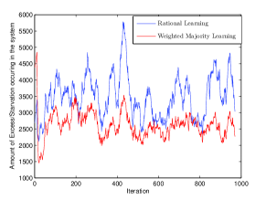
Figure 1: Resource excess/starvation occurring in the PP

3.3 Simulation Results

The Potluck Problem has been simulated with 100 non-identical agents with production capacities in the range of 500 to 1000 discrete units, and consumptions in the range of 0 to 1000, with 1000 instances of dinner. The mean consumption of all agents together came to 48,200. The mean production under rational learning was 47580, and under weighted majority learning was 48284. The weighted majority approach with the five simple predictors listed previously outperformed the rational approach about 99.5% of the time, and resulted in a level of starvation/excess that was 22.6% better than in the rational approach on average, and about 41.5% in the best case. (More intricate predictors are seen to yield even better results.) The results are depicted graphically in Figure 1.

4 Conclusion and Future Work

This paper proposed and analyzed the nature of the Potluck Problem. It is observed that a weighted majority learning approach results in better parity between demand and supply, compared to rational learning. Though in the present work, we have modeled the problem as only one resource being allocated/consumed, the problem can be easily extended by considering multiple resources, which are needed in specific, possibly unforeseen, proportions for better utility. In the current analysis, each agent chooses predictors from a pool of predictors available. This problem can be studied also by each agent choosing a different set of predictors from others, which closely resembles social behavior, and different sets of predictors can be compared and evaluated. Various predictor behaviors and performance can also be studied for specific patterns of demand, which can help in applying this model in a realistic scenarios.

References

- [1] Arthur, W. B. Inductive reasoning and bounded rationality. American Economic Review 84, 2 (1994), 406–411. This and other some related work may be seen at http://www.santafe.edu/arthur/Papers, the author’s web page.
- [2] Cournot, A. A. Recherches sur les Principes Mathématiques de la Théorie des Richesses. Calmann-Lévy, Paris, 1974. Originally published in 1838, this was re-printed (H. Guitton, ed.) as part of a collection titled Les Fondateurs.
- [3] Galstyan, A., Kolar, S., and Lerman, K. Resource allocation games with changing resource capacities. In Proceedings of the International Conference on Autonomous Agents and Multi-Agent Systems (AAMAS-2003) (2003).
- [4] Greenwald, A. R., Mishra, B., and Parikh, R. The Santa Fe Bar Problem revisited: Theoretical and practical implications, Apr. 1998. Unpublished Manuscript.
- [5] Littlestone, N., and Warmuth, M. K. The weighted majority algorithm. Information and Computation 108, 2 (Feb. 1994), 212–261.
- [6] Schaerf, A., Shoham, Y., and Tennenholtz, M. Adaptive load balancing: A study in multi-agent learning. Journal of Artificial Intelligence Research 2 (1995), 475–500.
- [7] Spees, K., and Lave, L. Demand response and electricity market efficiency. Carnegie Mellon Electricity Industry Center Working Paper CEIC-07-01 (Jan. 2007). Available at http://www.cmu.edu/electricity.