Thermodynamic behavior of the XXZ Heisenebrg $s=1/2$ chain around the factorizing magnetic field

Abstract

We have investigated the zero and finite temperature behaviors of the anisotropic antiferromagnetic Heisenberg XXZ spin-1/2 chain in the presence of a transverse magnetic field ($h$). The attention is concentrated on an interval of magnetic field between the factorizing field ($h_{f}$) and the critical one ($h_{c}$). The model presents a spin-flop phase for $0<h<h_{f}$ with an energy scale which is defined by the long range antiferromagnetic order while it undergoes an entanglement phase transition at $h=h_{f}$. The entanglement estimators clearly show that the entanglement is lost exactly at $h=h_{f}$ which justifies different quantum correlations on both sides of the factorizing field. As a consequence of zero entanglement (at $h=h_{f}$) the ground state is known exactly as a product of single particle states which is the starting point for initiating a spin wave theory. The linear spin wave theory is implemented to obtain the specific heat and thermal entanglement of the model in the interested region. A double peak structure is found in the specific heat around $h=h_{f}$ which manifests the existence of two energy scales in the system as a result of two competing orders before the critical point. These results are confirmed by the low temperature Lanczos data which we have computed.

1 Introduction

The zero temperature phase diagram (i.e. quantum phase diagram) of a model gives important information on the low temperature behaviors of the system [1, 2]. The anisotropic antiferromagnetic Heisenberg (XXZ) spin-1/2 model shows different quantum phases with respect to a symmetry-breaking transverse field (non-commuting magnetic field) [3, 4, 5]. The non-commuting field imposes quantum fluctuations into the ground state which can induce new phases. $Cs_{2}CoCl_{4}$ is a quasi-one dimensional spin-1/2 XY-like antiferromagnet with weak inter-chain couplings ($J^{\prime}/J=0.014$) which can be studied in terms of XXZ chain with anisotropy parameter $\Delta=0.25$ [6, 7]. The scaling behavior and quantum phase diagram of the XXZ model in the presence of a transverse magnetic field ($h^{x}$) have been investigated [3, 4, 5, 8].

Recently, the quantum spin models received much attentions from the quantum information point of views. These are prototype models to implement and examine the idea of quantum computations which requires the quantum correlations measured by entanglement. Hence, disentangled ground states have to be avoided for such implementations. On the other hand, the zero entanglement property of a ground state provides an exact form for it in terms of product of single particle states. The investigation in this direction resumed recently following the seminal work of J. Kurman and his collaboratores[9]. Several efforts have been devoted to this direction which is important for condensed matter researchers, i.e finding an exact (factorized) ground state even at particular values of the coupling constants [10, 11, 12, 13]. The factorized (exact) ground state is an accurate starting point to investigate the quantum nature of a phase close to the factorizing point in addition to some exact knowledge which gives at the factorized point. This property is implemented in this article to initiate a spin wave theory to describe the thermodynamic properties of the XXZ model in the presence of a transverse magnetic field.

The U(1) symmetry of the XXZ model is lost upon adding the transverse magnetic field. Initially, a perpendicular antiferromagnetic order is stabilized by promoting a spin-flop phase (which has a partial moment projection along the field direction). At the factorizing field ($h_{f}$) in the spin-flop phase the ground state is known exactly as a direct product of single spin states and the staggered magnetization along $y$-direction is close to its maximum value. In our model the factorizing field is $h_{f}=J\sqrt{2(1+\Delta)}$, where quantum fluctuations are uncorrelated and the ground state is the classical one ($J$ is the scale of energy and $\Delta$ is the anisotropy parameter). For slightly larger magnetic field very close to the critical one ($h_{f}<h<h_{c}$) the antiferromagnetic order becomes unstable and the staggered magnetization falls rapidly to vanish at the critical point. For $h>h_{c}$ the spins become aligned in $x$ direction and a fully polarized phase will be appeared. The region between the factorizing and the critical fields ($h_{f}<h<h_{c}$) is the main issue of our study which is not well understood so far.

The zero temperature properties of the intermediate region ($h_{f}<h<h_{c}$) induces its signature into the thermodynamic functions of the model. We have found that this region is characterized by two energy scales and its fingerprint will appear as a double peak in the specific heat. Moreover, the existence of more than an energy scale in the model can be related to a spontaneous symmetry breaking (SSB) [10]. Each broken phase is described by an order parameter which can be zero in the disordered phase. For the aforementioned model the symmetry breaking occurs where the staggered magnetization becomes zero.

The thermodynamic properties of the spin 1/2 XXZ chain in a transverse magnetic field have been studied using the Low temperature Lanczos method [15]. However, in this paper we will focus on the intermediate values of $h$ and more precisely on the region where a double peak appears in the specific heat of the model. We implement the exact factorized ground state at $h=h_{f}$ (where the entanglement vanishes) to build up a spin wave theory appropriate to describe the model in the intermediate values of the magnetic field. In the linear spin wave approximation we calculate the specific heat and thermal entanglement of the model. Moreover, the spin wave theory gives two different types of quasi particles which are representing the two energy scales. We have also studied both the zero and finite temperature properties of the model on a finite chain using the low temperature Lanczos method [14]. Our numerical results are in agreement with the spin wave theory counterparts. In the next section, we will briefly review the zero temperature properties of the model from the quantum information point of view. We will provide the spin wave theory in Sec.3 where the quantum property, specific heat and thermal entanglement are obtained. Finally, the numerical Lanczos results will be presented in addition to discussions on the mentioned topics.

2 Zero temperature phase diagram

The anisotropic spin-1/2 Heisenberg model in the presence of a transverse magnetic field is described by the following Hamiltonian,

$$H=J\sum_{i}(S_{i}^{x}S_{i+1}^{x}+S_{i}^{y}S_{i+1}^{y}+\Delta S_{i}^{z}S_{i+1}^{z}+hS_{i}^{x}),$$ (1)

where $S_{i}^{\alpha}$’s are spin-1/2 operators, $\Delta$ is the anisotropy parameter, $h$ is proportional to the transverse magnetic field and the exchange antiferromagnetic coupling $J$ which defines the scale of energy is set to one. This model has several quantum phases with respect to the transverse magnetic field and anisotropy parameter ($\Delta$). The $\alpha$-component spin structure factor at momentum $p$ is defined by

$$G^{\alpha\alpha}(p)=\sum_{x=1}^{N}\langle S_{1}^{\alpha}S_{1+x}^{\alpha}\rangle e^{ipx},$$ (2)

and its increasing behavior in term of system size shows the magnetic order at the specified momentum. We have plotted in Fig.(1) the magnetization along $x$ direction ($M_{x}=(1/N)\sum\langle S_{i}^{x}\rangle$) and the $y$-component of spin structure factor at momentum $p=\pi$ versus $h$. The value of $\Delta=0.25$ has been fixed to fit the case of real material $Cs_{2}CoCl_{4}$. The numerical data has been obtained by zero temperature Lanczos method on a finite chain of length $N=20$ with periodic boundary condition.

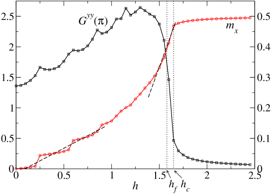
Figure 1: (color online) Results of numerical zero temperature Lanczos method for the magnetization along $x$-direction (right vertical axis) and the $y$-component spin structure factor at momentum $\pi$ (left vertical axis) versus the transverse magnetic field $h$ for a chain with $N=20$ and $\Delta$=0.25. The magnetization in $z$-direction is zero.

The magnetization curve can be distinguished in three parts: (1) Magnetization for $0<h<h_{f}$, (2) Magnetization for $h_{f}<h<h_{c}$, and (3) the paramagnetic phase for $h>h_{c}$. At zero magnetic field, there is no order in the system and all order parameters are zero i.e $M_{x,y,z}=0$. The nonzero value of $h$ starts to align the spins in $x$ direction and induces a small ferromagnetic order in $x$ direction. The magnetization, $M_{x}$, increases monotonically by increasing the magnetic field. For $h<h_{f}$ the quantum effects are considerable and the magnetization changes parabolically versus $h$. Increasing $h$, suppresses the quantum correlations and they goes to zero around $h_{f}$. For $h_{f}<h<h_{c}$, the magnetization is increased linearly versus $h$. Magnetization increases up to the critical point ($h_{c}$) and saturates at infinite field. Although the staggered magnetization along y-direction becomes zero at the finite critical field, the magnetization in x-direction will be fully saturated only for the isotropic case ($\Delta=1$) [13]. In other words, the full saturation in x-direction for $\Delta\neq 1$ will happen for $h\rightarrow\infty$. For $h>h_{c}$ all of spins align almost completely (for $\Delta\neq 1$) in the $x$ direction and we have a fully polarized paramagnetic phase.

We would like to draw your attentions to the region $h_{f}<h<h_{c}$, where the model behaves surprisingly. Let us first study the spin chain through the entanglement ($\tau_{2}$) of two spins [16, 17] which have no classical counterpart. The entanglement is defined by the following relation,

$$\tau_{2}=\sum_{i\neq j}C_{ij}^{2}\;.$$ (3)

Where, $C_{ij}$ is the concurrence [18] which is implemented instead of the pairwise zero temperature entanglement between two spins at sites $i$ and $j$. For $XXZ$ model, $M_{z}$ is zero thus the concurrence takes the form [17], $C_{ij}=2~{}max\{0,~{}C_{ij}^{(1)},~{}C_{ij}^{(2)}\},$ where

$$C_{ij}^{(1)} = \langle S_{i}^{x}S_{j}^{x}\rangle+|\langle S_{i}^{y}S_{j}^{y}\rangle-\langle S_{i}^{z}S_{j}^{z}\rangle|-\frac{1}{4},$$

$$C_{ij}^{(2)} = |\langle S_{i}^{y}S_{j}^{y}\rangle+\langle S_{i}^{z}S_{j}^{z}\rangle|-\sqrt{(\frac{1}{4}+\langle S_{i}^{x}S_{j}^{x}\rangle)^{2}-(M^{x})^{2}}.$$

Using quantum Monte Carlo simulation, T. Roscilde and collaborators [10] have shown that unlike the standard magnetic order parameters (Fig.1) the pairwise entanglement, plays an essential role at the factorizing field. At the factorizing field (also called classical field, $h_{cl}=h_{f}=\sqrt{2(1+\Delta)}$) [9] the ground state takes a product form [9, 13] and its entanglement is zero. In Fig.(2), we have plotted $C_{i,i+1}^{(1)}$ and $C_{i,i+1}^{(2)}$ versus the transverse field $h$ for XXZ spin-1/2 chain with $\Delta=0.25$ by using exact diagonalization Lanczos method. At the classical field ($h=h_{f}\simeq 1.58$), $C_{i,i+1}=C_{i,i+1}^{(1)}=C_{i,i+1}^{(2)}=0$. At this point the ground state of the model is factorized (disentangled) where the Neel order is roughly maximized in $y$ direction.

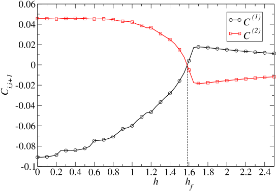
Figure 2: (color online) Entanglement estimators of the XXZ spin-1/2 chain versus transverse field $h$ with parameter $\Delta=0.25$. $C^{(1)}$ is depicted by (black) circles and $C^{(2)}$ by (red) squares. At the classical field ($h=h_{f}\simeq 1.58$), $C_{i,i+1}^{(1)}=C_{i,i+1}^{(2)}=0$.

Let us describe the behaviors of $C_{ij}^{(1)}$ and $C_{ij}^{(2)}$ from a spontaneous symmetry breaking (SSB) point of view. It is found in Ref. [10] that the competition between the two functions $C_{ij}^{(1)}$ and $C_{ij}^{(2)}$ demonstrates the appearance of a SSB. In other words, for our model, a SSB can be occurred when $C_{ij}^{(2)}<C_{ij}^{(1)}$. At this condition the magnetic field is greater than the factorizing value ($h>h_{f}$). Moreover, SSB is usually recognized to happen at the position where the order parameter becomes zero. In our model two standard order parameters, $M_{x}$ and $SM_{y}$ (staggered magnetization along $y$ direction) can represent the quantum phases of the model. We have plotted in Fig.(1) the magnetization along $x$ direction ($M_{x}$) and the $y$-component of spin structure factor ($G^{yy}$) at momentum $\pi$ for $\Delta=0.25$ XXZ spin-1/2 chain. $M_{x}$ is nonzero in the whole range of magnetic fields however, $G^{yy}(\pi)$ which is used to show the antiferromagnetic order of the system has a different behavior. As it is observed from our Lanczos data, $G^{yy}(\pi)$ increases by $h$ up to $h_{f}$. This behavior is also found in the $SM^{y}$ curve which has been obtained by density matrix renormalization group (DMRG) [8]. Thus, no SSB occurs for $h<h_{f}$. By increasing the magnetic field for $h>h_{f}$, $G^{yy}(\pi)$ (or equivalently $SM_{y}$) decreases rapidly and falls to zero at the critical point $h_{c}$. In this respect, a symmetry breaking can occur only for $h>h_{f}$. In this region, as mentioned before the slop of $M_{x}$ with respect to $h$ is different from the corresponding one for $h<h_{f}$.

3 Spin waves theory

As discussed in the previous section the entanglement is zero at the factorizing field ($h_{f}$). It allow s us to write the many body ground state as the direct product of the single spin states on odd and even sublattices [9]

$$|GS\rangle=\bigotimes_{i\in odd,j\in even}|S_{i}\rangle|S_{j}\rangle$$ (5)

The spin state on each sublattice is expressed in terms of polar angles ($\theta,\phi$) which defines the rotation of the up-spin eigen-state of $S^{z}$ to the specific direction defined by the factorized state. Let us label the odd (even) sublattice by $A(B)$. Thus, ($\theta,\phi$) represents A-sublattice while ($\beta,\alpha$) is the corresponding one for B-sublattice. It has been shown [13] that one can consider $\phi=0=\alpha$ without loss of generality. Moreover, the magnitude of remaining polar angles are equal $|\theta|=|\beta|$ in the case of homogeneous spin model (like here) and is given by

$$\cos(\theta)=-\sqrt{\frac{1+\Delta}{2}}$$ (6)

For the antiferromagnetic model the factorized ground state is defined by $\beta=-\theta$.

Before starting the spin wave approach we implement a unitary transformation on the Hamiltonian. All spins on the A-sublattice are rotated with angle $\theta$ counterclockwise around y-direction and clockwise for spins on B-sublattice. The rotated Hamiltonian ($\tilde{H}$) is the result of rotations on all lattice points, $\tilde{H}=\tilde{D}^{{\dagger}}H\tilde{D}$ and $\tilde{D}=\bigotimes_{i\in A,j\in B}{\cal D}_{i}(-\theta){\cal D}_{j}(\theta)$. The single spin rotation operator is ${\cal D}_{i}(\theta)=exp(-i\theta S_{i}^{y}/\hbar)$. In the rotated spin model, the Hamiltonian will have a factorized ground state which is a ferromagnet at the factorizing field. The rotated spin Hamiltonian is written in terms of boson operators $a,b$ with the following Holstein-Primakoff transformation,

$$\tilde{S}_{Ai}^{+} = (2S-a_{i}^{\dagger}a_{i})^{1/2}a_{i},~{}~{}~{}~{}~{}~{}~{}~{}~{}\tilde{S}_{Ai}^{x}=S-a_{i}^{\dagger}a_{i},$$

$$\tilde{S}_{Bj}^{+} = (2S-b_{j}^{\dagger}b_{j})^{1/2}b_{j},~{}~{}~{}~{}~{}~{}~{}~{}~{}\tilde{S}_{Bj}^{x}=S-b_{j}^{\dagger}b_{j},$$

where $\tilde{S}_{A(B)}={\cal D}_{A(B)}^{\dagger}S_{A(B)}{\cal D}_{A(B)}$ are the rotated spin operators and ${\cal D}_{A(B)}$ is the unitary single spin rotation operator. The bosonic Hamiltonian in the linear spin wave approximation, i.e. $\tilde{S}_{Ai}^{+}\simeq\sqrt{2S}a_{i};\tilde{S}_{Bi}^{+}\simeq\sqrt{2S}b_{i}$, is given by

$$\tilde{{\cal H}}=N[\frac{\Delta}{2}+\frac{h}{h_{f}}(1+\Delta)]+\sum_{l=0}^{N}\bigg{(}[\frac{h}{h_{f}}(1+\Delta)-\Delta](a_{l}^{\dagger}a_{l}+b_{l}^{\dagger}b_{l})$$

$$-\frac{\Delta}{2}[a_{l}(b_{l}^{\dagger}+b_{l+1}^{\dagger})+h.c]+\frac{1}{2}(\frac{h}{h_{f}}-1)\sqrt{1-\Delta^{2}}(a_{l}+b_{l}+h.c)\bigg{)}.$$ (7)

To diagonalize the bosonic model we first implement the Fourier transformation and then apply a rotation to the boson operators ($a_{k},b_{k}$)

$$a_{l}=\frac{1}{\sqrt{N}}\sum_{k}e^{-ikl}a_{k},$$

$$b_{l}=\frac{1}{\sqrt{N}}\sum_{k}e^{-i(kl+\frac{k}{2})}b_{k},$$

$$\psi_{k} = \cos\eta_{k}a_{k}-\sin\eta_{k}b_{k},$$

$$\chi_{k} = \sin\eta_{k}a_{k}+\cos\eta_{k}b_{k}.$$ (8)

The diagonalized Hamiltonian in terms of two sets of quasi-particle operators is given by

$$\tilde{{\cal H}}=E_{0}+\sum_{k}(\omega_{k}^{+}\chi_{k}^{\dagger}\chi_{k}+\omega_{k}^{-}\psi_{k}^{\dagger}\psi_{k}),$$ (9)

where the excitation spectrums have the following forms

$$\omega_{k}^{\pm}=\frac{h}{h_{f}}(1+\Delta)-\Delta\pm\Delta\cos\frac{k}{2},$$

$$E_{0}=\frac{N}{2}(\Delta-hh_{f})+\omega_{0}^{+}(t^{+})^{2}+\sqrt{2N(1-\Delta^{2})}(\frac{h}{h_{f}}-1)t^{+},$$

$$t^{+}=\frac{\sqrt{\frac{N}{2}(1-\Delta^{2})}(1-\frac{h}{h_{f}})}{\omega_{0}^{+}}.$$ (10)

In the above calculations, a translation $\chi_{0}\rightarrow\chi_{0}+t^{+}$ has been performed in the diagonalization procedure of the Hamiltonian (7).

The Hamiltonian is now represented in terms of two quasi-particles (bosons), each defines an energy scale. The two energy scales which are the excitation energies of each bosons lead to two different dynamics for the system. The consequence of two types of dynamics will be seen in the structure of specific heat which will be studied. However, the existence of two different quasi-particle energies ($\omega_{k}^{+}\neq\omega_{k}^{-}$) is the first sign of two dynamics in the model.

3.0.1 Specific heat

To get the finite temperature properties of the model, we assume $\tilde{n}_{k}^{\pm}=\sum_{n^{-},n^{+}}n_{k}^{\pm}P_{k}(n^{+},n^{-})$, for the spin wave distribution functions, where $P_{k}(n^{+},n^{-})$ is the probability of parallel ($n_{k}^{+}=\chi^{\dagger}_{k}\chi_{k}$) and perpendicular ($n_{k}^{-}=\psi_{k}^{\dagger}\psi_{k}$) normal modes appearing in the $k$-momentum state which satisfies $\sum_{n^{+},n^{-}}P_{k}(n^{+},n^{-})=1$ for all $k$’s. The substitutions of $\tilde{n}^{+}_{k}=\langle\chi^{\dagger}_{k}\chi_{k}\rangle$ and $\tilde{n}_{k}^{-}=\langle\psi_{k}^{\dagger}\psi_{k}\rangle$ (where $\langle\cdots\rangle$ represents the thermal average) in the spin-wave Hamiltonian (9) gives the free energy,

$$F = E_{0}+\sum_{k}(\omega_{k}^{+}\tilde{n}_{k}^{+}+\omega_{k}^{-}\tilde{n}_{k}^{-})+T\sum_{k}\sum_{n^{+},n^{-}}P_{k}(n^{-},n^{+})\ln P_{k}(n^{-},n^{+}).$$

The number of bosons are controlled by the following constraint which is the magnetization in x-direction,

$$M_{x}=s-\frac{1}{2N}\sum_{k}(\tilde{n}_{k}^{+}+\tilde{n}_{k}^{-})-\frac{(t^{+})^{2}}{2N}.$$ (11)

The free energy is minimized with respect to $P_{k}(n^{+},n^{-})$s under the constraint of (11) which is applied by a Lagrange multiplier ($\mu$) via the boson’s occupation number

$$\tilde{n}_{k}^{\pm}=\frac{1}{e^{\frac{1}{k_{B}T}(\omega^{\pm}-\mu)}-1}.$$ (12)

The constraint (11) is applied by the values of $M_{x}(h,T)$ which have been obtained by the numerical Lanczos method. We have plotted in Fig.(3) the specific heat of $\Delta=0.25$ XXZ spin-1/2 chain versus temperature and different values of magnetic field. A double peak is observed in the specific heat which is the signature of the existence of two comparable energy scales. More precisely, the specific heat for $h=1.4\;\mbox{and}\;1.5$ have a narrow peak at low temperature ($T\simeq 0.2$) and a broaden one at higher $T$. We will discuss more on this point in the next section.

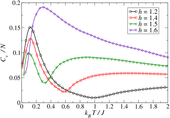
Figure 3: (color online) The spin wave results for specific heat of the XXZ model versus $T$ for different values of the transverse magnetic field $h$ and anisotropy parameter $\Delta=0.25$. (Black) circle is for $h=1.2$, (red) square: $h=1.4$, (green) gradient: $h=1.5$ and (blue) diamond: $h=1.6$. A narrow peak at low temperature followed by a broaden one for higher temperature are observed for $h=1.4,1.5$.

3.0.2 Thermal entanglement

The established spin wave theory close to the factorizing point is used to obtain the thermal behaviors of the correlation functions in Eqs.(LABEL:concurrence) and consequently to calculate the concurrence. This method can describe the thermal entanglement of two spins in linear spin wave approximation. In this approach, one can find the following expression for $C_{ij}^{(1)}$ and $C_{ij}^{(2)}$

$$C_{ij}^{(1)}\simeq-\frac{1}{2N}\bigg{(}\sum_{k}(\tilde{n}_{k}^{+}+\tilde{n}_{k}^{-})+(t^{+})^{2}\bigg{)},$$

$$C_{ij}^{(2)}\simeq\frac{1}{2N}\bigg{(}\sum_{k}Cos(k\cdot r+k/2)(\tilde{n}_{k}^{+}-\tilde{n}_{k}^{-})+(t^{+})^{2}\bigg{)}.$$

As it is seen from these functions, $C_{ij}^{(1)}$ is always less than zero thus the concurrence is $2~{}max\{0,C_{ij}^{(2)}\}$. We have plotted in Fig.(4) the thermal entanglement of the $\Delta=0.25$ XXZ spin-1/2 chain versus transverse field at temperature $T=0.05$. By increasing the magnetic field, quantum fluctuations are decreased and the thermal entanglement is declined. At the factorizing point, quantum fluctuations become approximately uncorrelated and the thermal entanglement is very close to zero ($\sim 10^{-3}$). It means that the thermal entanglement is mainly originated from the ground state and the excited states have very tiny contribution to the entanglement.

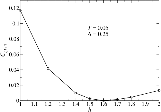
Figure 4: Thermal entanglement of the XXZ model versus $h$ and anisotropy parameter $\Delta=0.25$ at $T=0.05$ which has been obtained by spin wave approximation. Because of the tiny contribution of excited states to the entanglement, its value at $h_{f}$ is $\sim 10^{-3}$.

4 Summary, Discussions and Lanczos results

We have studied the effects of transverse magnetic field on the zero and finite temperature properties of $\Delta=0.25$ XXZ spin-1/2 chain. We have focused our attentions on the intermediate region of $h_{f}<h<h_{c}$ where the model behaves more interestingly.

M. Kenzelmann and his collaborators [6] have investigated experimentally the effects of a transverse magnetic field on the quasi-one dimensional spin-1/2 antiferromagnet $Cs_{2}CoCl_{4}$, using single-crystal neutron diffraction. Due to the weak inter-chain couplings in $Cs_{2}CoCl_{4}$ ($J^{\prime}/J=0.014$) [7] where $J$ is the coupling within a chain, it is proposed in Ref. [6] that the bulk material has a spin liquid phase at the interval $h_{f}<h<h_{c}$. In a spin liquid phase all order parameters should be zero and there should be no long range order in the system. The existence of very weak coupling between magnetic chains in this material makes it feasible to be described by a one dimensional spin-1/2 XXZ model with the anisotropy parameter $\Delta=0.25$. However, for the 1D XXZ model in the region $h_{f}<h<h_{c}$ both magnetization and staggered magnetization are nonzero. Thus the ground state of the model could not be a spin liquid phase. Although the behaviors of the magnetic orders for this region are clearly known, the lacuna of a perfect study of the properties of the system at the intermediate region is still felt. In this respect, we have devoted our attentions to survey the magnetic and thermodynamic behavior of the system at the intermediate region of the transverse field.

We have implemented the low temperature Lanczos method (LTLM) [14, 15] to compute the thermodynamic behaviors of the model for a chain of finite length. LTLM has been used since it is accurate for low temperatures and specially the thermodynamic averages reach the ground state expectation values as temperature approaches zero. The specific heat versus temperature for different values of the magnetic field on a chain of $N=20$ and with $\Delta=0.25$ has been plotted in Fig. (5). The sampling is taken over $R=100$ Lanczos numerical data which have been obtained by different initial random states. The finite size effect can be ignored since the number of sampling ($R$) is rather high. The result of the spin wave theory (Fig.3) and LTLM (Fig.5) are in mutual agreement; moreover, both figures show the presence of double peak in the specific heat for $h=1.4,1.5$ which is an evidence for the existence of two scales of energy or equivalently two dynamics in the system.

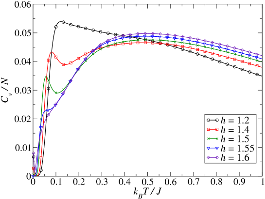
Figure 5: The numerical Lanczos results for the specific heat of XXZ model versus $T$ for different values of transverse magnetic field and $\Delta=0.25$. At the intermediate region of $h$, a double peak structure is observed which indicates the existence of two energy scales in the system.

The specific heat versus $T$ for all values of the magnetic fields has Schottky like peak at low temperatures which is a remarkable feature of the antiferromagnetic behavior. For small values of the magnetic field ($h<1.4$) the Schottky anomaly is the only one which justifies the existence of a single dynamics in the model. Further increasing of the magnetic field (being close to the factorizing point) a broaden peak is emerged in the specific heat data versus $T$. This bump is the result of the paramagnetic order. Two different orders are in competition and its signature is specially observable for magnetic fields in the region $h_{f}\lesssim h<h_{c}$ where the magnitude of the two types of ordering becomes comparable. The antiferromagnetic order in y-direction is the result of exchange coupling in the broken U(1) symmetry phase. The effect of transverse magnetic field as a paramagnetic order in x-direction shows its presence when it is enough large to define a new scale of energy. Around the factorizing field the two orders manifest their influence on the model as a narrow and broaden peak of the specific heat which happens for $h_{f}\lesssim h<h_{c}$. This is the region where the spontaneous symmetry breaking is started to happen. At the critical point ($h_{c}$) the antiferromagnetic order vanishes and paramagnetic order is the only representative of the model. A broaden peak in the specific heat versus $T$ is significant for $h>h_{c}$ which justifies the paramagnetic order.

Employing the specific heat data, one can also scan the behavior of the energy gap ($E_{g}$). The existence of energy gap in the model is clearly observed by the exponential decay of the specific heat at very low temperatures ($T\lesssim 0.02$).

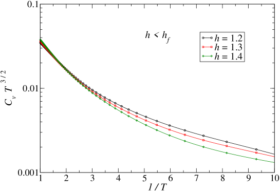
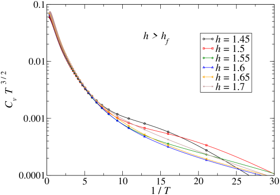
Figure 6: $c_{v}T^{3/2}$ of XXZ model versus $1/T$ for different values of $h<h_{f}$ and $\Delta=0.25$. At low temperatures the slope of the curve shows increasing of the energy gap in the system.

Figure 7: $c_{v}T^{3/2}$ of XXZ model versus $1/T$ for different values of $h>h_{f}$ and $\Delta=0.25$. At low temperatures, the slop of the curve is decreased from $h=1.45$ to $h=1.6$ and then starts to increase by increasing of $h$.

At enough low temperatures ($T<E_{g}$) the specific heat and energy gap are related by [7]

$$c_{v}T^{3/2}\propto e^{-\frac{E_{g}}{T}}.$$ (13)

Thus, the slop of ($c_{v}T^{3/2}$) curves versus $\frac{1}{T}$ in log scale gives good information about the energy gap. In Figs.(7,7) we have plotted ($c_{v}T^{3/2}$) versus $\frac{1}{T}$ for different values of transverse field. Fig.(7) shows the gap behavior close to the factorizing point, $h<h_{f}$. While its behavior for $h>h_{f}$ is presented in Fig.(7). A turning point of different plots in Fig.(7) for different transverse magnetic field is the result of different behavior for $h<h_{c}\simeq 1.65$ (decreasing gap) and $h>h_{c}$ (linear increasing paramagnetic gap). Our results fit very well with Figs. (5.14 and 5.15) of Ref. [7].

Motivated by neutron-scattering results [6], T. Radu [7] investigated the effects of non-commuting field on the ground state of $Cs_{2}CoCl_{4}$. To be more precise in comparison, let us refer also to Fig.13 of chapter.5 of Ref. [7] where the experimental data of the specific heat have been shown. The experimental data (specially in the inset of Fig.13 of chapter.5 of Ref.[7]) display a double peak in the specific heat versus temperature which is for the intermediate range of magnetic field (less than the critical one).

It is also worth to point out the behaviors of the system from the internal energy points of view. The internal energy and specific heat are related by relation $C=\frac{dU}{dT}$. The double peak structure of the specific heat presages that at the intermediate values of the transverse field, there are two temperatures where the internal energy of the system gets its maximum variation. In other words, at these temperatures the maximum amount of states contribute to the response functions of the systems. Thus, one can also conclude that the appearance of the two energy scales in the system is appropriate with the number of contributed states. Knowledge on these properties could be important in the study of the magneto-caloric effects of the XXZ model in the transverse field which is a work in progress.

References

References

- [1] Sachdev S 1999 Quantum phase transitions, Cambridge University Press, Cambridge, UK
- [2] Vojta M 2003 Rep. Prog. Phys. 66
- [3] Dmitriev D V, Krivnov V Ya and Ovchinnikov A A 2002 Phys. Rev. B 65 172409 ; Dmitriev D V, Krivnov V Ya, Ovchinnikov A A and Langari A 2002 JETP 95 538
- [4] Langari A 2004 Phys. Rev. B 69 100402(R)
- [5] Langari A and Mahdavifar S 2006 Phys. Rev. B 73 54410
- [6] Kenzelmann M, et al. 2002 Phys. Rev. B 65 144432
- [7] Radu T 2005 Thermodynamic characterization of Heavy fermion systems and low dimensional quantum magnets near a quantum critical point, Ph. D. Thesis, Max Planck Institute for chemical physics of solids
- [8] Caux Jean-Se´·bastien, Essler Fabian H L and Löw Ute 2003 Phys. Rev. B 68 134431
- [9] Kurmann J, Thomas H and Muller G 1982 Physica 112 A 235
- [10] Roscilde T, Verrucchi P, Fubini A, Haas S and Tognetti V 2004 Phys. Rev. Lett. 93 167203
- [11] Giampaolo S M, Adesso G, and Illuminati F 2008 Phys. Rev. Lett. 100 197201
- [12] Giampaolo S M, Adesso G and Illuminati F 2009 Phys. Rev. B 79 224434
- [13] Rezai M, Langari A and Abouie J 2010 Phys. Rev. B 81 060401(R)
- [14] Aichhorn M, Daghofer M, Evertz H and Linden W Von der 2003 Phys. Rev. B 67 161103(R)
- [15] Siahatgar M and Langari A 2008 Phys. Rev. B 77 054435
- [16] Coffman V et al. 2000 Phys. Rev. A 61 052306
- [17] Amico L et al. 2004 Phys. Rev. A 69 022304
- [18] Wootters W K 1998 Phys. Rev. Lett. 80 2245
- [19] Wang Y R 1992 Phys. Rev. B 45 12604(R)