ADS/CFT Applied To Vector Meson Emission From A Heavy Accelerated Nucleus

Abstract

We consider a classical source, moving on the 4-D boundary of a 5-D ADS space, that is coupled to quantum fields residing in the bulk. Bremsstrahlung-like radiation of the corresponding quanta is shown to occur and the S-matrix is derived assuming that the source is sufficiently massive so that recoil effects are negligible. As an illustrative example, using the ADS hard-wall model, we consider vector mesons coupled to a heavy nucleus that is moved around at high speed in an accelerator ring. The meson radiation rate is found to be finite but small. Much higher accelerations, such as when a pair of heavy ions suffer an ultra peripheral collision, cause substantial emission of various excited vector mesons. Predictions are made for the spectrum of this radiation. A comparison is made against existing photon-pomeron fusion calculations for the transverse momentum spectra of rho mesons. These have the same overall shape as the recently measured transverse momentum distributions at RHIC.

The gauge/gravity correspondence[1] is a powerful means for extracting information about four-dimensional strongly coupled gauge theories by mapping them onto gravitational theories in five dimensions where, because of the weak coupling, they may be solved much more easily. A highly prized goal is to learn about non-perturbative QCD from some 5-D theory. This goal is still some distance away because the gravity theory actually dual to QCD is not yet known. Nevertheless, using variants of the $N=4$ supersymmetric models, there have been a large number of interesting applications . These include hard QCD scattering and deep inelastic structure functions[2], low lying hadron spectra[3], chiral symmetry breaking[4], vector-meson couplings[5]; meson form factors[6] moments of generalized parton distribution [7], kaon decays[8], etc. There are many valid criticisms of the holographic approach[9] but, on the whole, the reasonable agreement with experiment suggests that ADS ideas deserve further exploration.

This work aims at extending the range of problems to which ADS ideas have been applied. Since this is an illustrative calculation, for simplicity we shall use the well-known hard-wall model. This uses an abrupt cutoff in ADS space. While unsatisfactory in describing meson Regge trajectories, it is the simplest way of enforcing confinement in this ”bottom-up” approach. However, it should be possible to generalize the contents of this paper to the ”soft-wall”, designed to give the correct Regge behaviour [4]. We choose vector fields since they have the simplest ADS description.

Let us quickly review the standard ADS approach to QCD: the gravity theory is defined on a (d+1)-dimensional Anti-de Sitter $AdS_{d+1}$ space with a $d$-dimensional asymptotic boundary at $z=0.$ The fields $\Phi(z,x)$ propagate in $AdS_{d+1}$ and approach  the conformal field theory (CFT) fields $\Phi_{0}(x)$ on the boundary. Various QCD composite operators $J(x)$, which are built from quark and gluon operators and exist only on $z=0$, act as sources for $\Phi(z,x).$ They essentially serve as mathematical devices by which to probe the bulk. On the gravity side the generating functional is,

$$Z_{grav}=e^{iS_{eff}[\Phi]}=\int D\Phi e^{i\Phi},$$

while on the CFT side, in the presence of the operator probes $J(x)$,

$$Z_{CFT}=e^{iS_{CFT}[\Phi_{0}]}=\int D\Phi e^{iS_{QCD}+i\int d^{d}xJ(x)\Phi_{0}(x)}.$$

The duality between the physics on the boundary and in the bulk is then succinctly expressed by the equality,

$$Z_{grav}[\Phi\rightarrow\Phi_{0}]=Z_{CFT}[\Phi_{0}]$$

In the supergravity approximation, $Z_{grav}$ is easily calculated. Functional differentiation with respect to $J(x)$ yields the desired correlation functions of fields such as $\left\langle\Phi_{0}(x)\Phi_{0}(x^{\prime})\right\rangle.$ With $J(x)$ having served its purpose, it can be set equal to zero.

The approach taken here will be slightly different. We shall take $J(x)$ to be an isovector source that excites fields in the bulk with the right quantum numbers. However it will be a ”real” source, not a fictitious one. This is analogous to a time varying electrical current that couples to the electromagnetic field and radiates photons. Provided that the energy radiated is small, the recoil is negligible. Similarly, we shall assume that the back-reaction on the iso-vector source radiating vector mesons can also be ignored. The limitaions of this approach will be discussed.

1 S-Matrix

With $R$ as the curvature of the AdS₅ space, the metric has the conventional form,

$$ds^{2}=\frac{R^{2}}{z^{2}}(\eta_{\mu\nu}dx^{\mu}dx^{\nu}-dz^{2}),\text{ for }z_{0}>z>0.$$ (1)

where $\eta_{\mu\nu}=(1,-1,-1,-1),$ $z=0$ is the 4-dimensional world sheet, and $z_{0}$ is the distance at which the AdS₅ ends. The indices $\mu,\nu$ run from 0 to 3 while AdS₅ indices, denoted by $m,n$ run over 0, 1, 2, 3, $z$. Limiting our attention to vector mesons, the bulk action is,

$$S =-\frac{1}{4g_{5}^{2}}\int d^{5}xTr[F^{mn}F_{mn}]$$ (2)

$$F_{mn} =\partial_{m}A_{n}-\partial_{n}A_{m}-i[A_{m},A_{n}].$$ (3)

The field $A_{m}$ transforms under flavour $SU(N)$, $A_{m}=A_{m}^{a}t^{a}.$ Suppressing the flavour index, and with the gauge choice $A_{z}(z,x)=0,$ the linearized equation of motion reads,

$$[z\partial_{z}(z^{-1}\partial_{z})-\square]A^{\mu}=0$$ (4)

with $\square=\partial^{\mu}\partial_{\mu}$ being the usual D’Alembertian operator. As the boundary condition, we require that $A^{\mu}(0,x)\ =0$ and that $F_{mn}$ vanish at $z=z_{0}.$ The latter implies the Neuman boundary condition, $\frac{\partial A^{\mu}}{\partial z}=0.$ Both conditions are satisfied by $A^{\mu}=\varepsilon^{\mu}e^{-ik\cdot x}zJ_{1}(kz)$ for any $k$ that satisfies $J_{0}(kz_{0})=0.$ Since $k^{2}=k^{\mu}k_{\mu}=m^{2}$, this implies a tower of vector mesons with masses given by $m_{p}=\frac{\chi_{p}}{z_{0}}$, where $J_{0}(\chi_{p})=0,\;p=1,2,\cdot\cdot\cdot$

Thus, the most general solution of Eq. 4 is,

$$A^{\mu}(z,x)=\sum_{p=1,\lambda}^{\infty}\int\frac{d^{4}k}{(2\pi)^{4}}a_{p}(k,\lambda)\varepsilon^{\mu}(k,\lambda)e^{-ik\cdot x}zJ_{1}(kz)2\pi\delta(k^{2}-m^{2})+cc.$$ (5)

Canonical quantization now follows in a rather obvious way[10] by imposing the commutation relation,

$$\left[a_{p}(k,\lambda),a_{p^{\prime}}^{\dagger}(k^{\prime},\lambda^{\prime})\right]=\delta_{pp^{\prime}}\delta_{\lambda\lambda^{\prime}}\delta^{3}(k-k^{\prime}).$$ (6)

This leads to,

$$\left[A^{\mu}(z,x),A^{\mu^{\prime}}(z^{\prime},x^{\prime})\right] =zz^{\prime}\sum_{p=1}^{\infty}\frac{1}{z_{0}^{2}c_{p}^{2}}\triangle_{p}^{\mu\mu^{\prime}}(x-x^{\prime})J_{1}(k_{p}z)J_{1}(k_{p}z^{\prime}),$$ (7)

$$\triangle_{p}^{\mu\mu^{\prime}}(x) =\int d\widetilde{k_{p}}\left(e^{-ik\cdot x}-e^{ik\cdot x}\right)(-g^{\mu\mu^{\prime}}+\frac{k^{\mu}k^{\mu^{\prime}}}{k^{2}}),$$ (8)

$$c_{p}^{2} =\int_{0}^{1}dyyJ_{1}^{2}(\chi_{p}y)$$ (9)

$$d\widetilde{k_{p}} =\frac{d^{3}k}{(2\pi)^{3}2\omega_{p}}\text{ with }\omega_{p}^{2}=\left|\overrightarrow{k}\right|^{2}+m_{p}^{2}.$$ (10)

The above sum over momenta is restricted to discrete values, $k_{p}=\frac{\chi_{p}}{z_{0}}$.

The field in the bulk arising from a source $J^{\mu}(x)$ placed on the $z=0$ boundary is,

$$A^{\mu}(z,x)=g\int d^{4}xG(z,x-x^{\prime})J^{\mu}(x^{\prime}),$$ (11)

where the Green’s function $G(z,x-x^{\prime})$ is a sum of retarded and advanced parts, $G=G_{R}+G_{A}$. It will be computed using the basis provided by the solutions of Eq. 4.

To this end, let us find solutions to

$$[z\partial_{z}(z^{-1}\partial_{z})-\square]G(z,x)=\delta^{4}(x-x^{\prime}).$$ (12)

After Fourier transformation, the solution can be written as,

$$G(z,x)=\int\frac{d^{4}k}{(2\pi)^{4}}e^{-ik\cdot x}zf(k,z),\text{ \ }$$ (13)

where $f(k,z)$ obeys,

$$\left[z^{2}\frac{d^{2}}{dz^{2}}+z\frac{d}{dz}+(k^{2}z^{2}-1)\right]f(k,z)=z.$$ (14)

With the boundary conditions $f(k,0)=0$ and $(zf)^{\prime}\!(z=z_{0})=0$ , Eq. 14 yields a complete, orthogonal set of solutions $\left\{J_{1}(k_{p}z)\right\}$ which allow for the delta function expansion,

$$\frac{1}{z}\delta(z-z^{\prime})=\frac{1}{z_{0}^{2}}\sum_{p=1}^{\infty}J_{1}(k_{p}z)J_{1}(k_{p}z^{\prime}).$$ (15)

Using this, the solution of 14 is then easily seen to be,

$$f(k,z)=\sum_{p=1}^{\infty}\frac{1}{z_{0}^{2}c_{p}^{2}}\int_{0}^{z_{0}}dz^{\prime}\frac{J_{1}(k_{p}z)J_{1}(k_{p}z^{\prime})}{k^{2}-k_{p}^{2}}.$$ (16)

Thus, one arrives at the following final form for the Green’s function,

$$G(z,x)=\frac{1}{z_{0}}\sum_{p=1}^{\infty}\alpha_{p}G_{p}(x)zJ_{1}(k_{p}z)$$ (17)

where,

$$G_{p}(x) =\int\frac{d^{4}k}{(2\pi)^{4}}\frac{e^{-ik\cdot x}}{k^{2}-k_{p}^{2}},$$ (18)

$$\alpha_{p} =\frac{\int_{0}^{1}dxJ_{1}(x\chi_{p})}{\int_{0}^{1}dxxJ_{1}^{2}(x\chi_{p})}$$ (19)

We shall now follow the procedure described by Itzykson and Zuber to find the S-matrix that connects the fields before and after interaction with a time-dependent source[11]. So imagine that the source, which obeys $\partial_{\mu}J^{\mu}=0$, is turned on for a finite time $-T<t<T$. The ”in” and ”out” fields, defined as $A_{in}^{\mu}=\lim_{t\rightarrow-\infty}A^{\mu}$ and $A_{out}^{\mu}=\lim_{t\rightarrow\infty}A^{\mu},$ are related by,

$$A_{out}^{\mu}(z,x)=A_{in}^{\mu}(z,x)+\int d^{4}x^{\prime}G^{-}(z,x-x^{\prime})J^{\mu}(x^{\prime}),\text{ }$$ (20)

where $G^{-}\equiv G^{R}-G^{A}$ and $G^{R},G^{A}$ are, respectively, the retarded and advanced Green’s functions. $G^{-}$ is trivially obtained from Eq.17 in terms of the Green’s functions for individual modes,

$$G^{-}(z,x) =\frac{1}{z_{0}}\sum_{p=1}^{\infty}\alpha_{p}G_{p}^{-}(x)zJ_{1}(k_{p}z),$$ (21)

$$G_{p}^{-}(x) =G_{p}^{R}-G_{p}^{A}$$

$$=i\int d\widetilde{k_{p}}\left(e^{-ik\cdot x}-e^{ik\cdot x}\right)$$ (22)

The incoming and outgoing fields are also connected through a unitary operator $S,$

$$A_{out}^{\mu}(z,x)=S^{-1}A_{in}^{\mu}(z,x)S,$$ (23)

for which the following ansatz can be made,

$$S=e^{-i\int d^{4}xdzh(z)J_{\mu}(x)A^{\mu}(z,x)}$$ (24)

where $h(z)$ is as yet an unknown function. From the field commutation relation in Eq.7, and from the Baker-Campbell-Haussdorf relation, $e^{A}Be^{-A}=B+[A,B]$ (which holds for $[A,[A,B]]=0),$ it follows that,

$$A_{out}^{\mu}(z,x) =S^{-1}A_{in}^{\mu}(z,x)S=A_{in}^{\mu}(z,x)+$$ (25)

$$\sum_{p=1}^{\infty}\int d^{4}x^{\prime}dz^{\prime}f(z^{\prime})\frac{zz^{\prime}}{z_{0}^{2}c_{p}^{2}}J_{1}(k_{p}z)J_{1}(k_{p}z^{\prime})G_{p}^{-}(x-x^{\prime})J^{\mu}(x^{\prime}).\qquad$$

Setting equal the expressions for $A_{out}^{\mu}(z,x)$ in Eq.20 and Eq.25 forces the choice $h(z)=z^{-1}$ and leads to the important result,

$$S=e^{-i\int d^{4}x\frac{dz}{z}J_{\mu}(x)A^{\mu}(z,x)}.$$ (26)

From the asymptotic behaviour of $J_{1}(kz)$ for small $z$, it is clear that the integrand above does not contain any singularity.

From the S-matrix derived in Eq.26 above one can compute the amplitude for the current $J_{\mu}(x)$ to produce any number of vector mesons. Because $A^{\mu}(z,x)$ in Eq.5 contains both creation $($inside $A_{\mu}^{-})$ and destruction $($inside $A_{\mu}^{+})$ operators, it is first necessary to separate these by using the identity $e^{A+B}=e^{A}e^{B}e^{-[A,B]/2}$. This gives,

$$S =e^{-ig\int d^{4}x\frac{dz}{z}J^{\mu}(x)A_{\mu}^{-}(z,x)}e^{-ig\int d^{4}x\frac{dz}{z}J^{\mu}(x)A_{\mu}^{+}(z,x)}$$ (27)

$$\times e^{-g^{2}\sum_{p=1}^{\infty}\beta_{p}^{2}\int d\widetilde{k_{p}}\overrightarrow{J}^{\ast}(k)\cdot\overrightarrow{J}(k)}$$ (28)

where,

$$\beta_{p}^{2}=\frac{\left[\int_{0}^{1}dxJ_{1}(x\chi_{p})\right]^{2}}{\int_{0}^{1}dxxJ_{1}^{2}(x\chi_{p})},$$ (29)

and $\overrightarrow{J}(k)$ is the 4-d Fourier transform of $\overrightarrow{J}(x),$

$$\overrightarrow{J}(k)=\int d^{4}xe^{-ik\cdot x}\overrightarrow{J}(x).$$ (30)

Note that $\overrightarrow{J^{\ast}}(k)=$ $\overrightarrow{J}(-k)$ and that only the physical polarizations have entered the calculations.

The probability for producing a single vector meson with polarization $\lambda,$excitation $p$, and located in the momentum space element $d^{3}k$ is easily obtained from Eq.27 ,

$$dP =\left|A\right|^{2}d\widetilde{k_{p}}=\left|A\right|^{2}\frac{d^{3}k}{(2\pi)^{3}2\omega_{p}}$$ (31)

$$A =-ig\beta_{p}\frac{\varepsilon(k,\lambda)\cdot J(k)}{Exp[g^{2}\sum_{p=1}^{\infty}\beta_{p}^{2}\int d\widetilde{k_{p}}\overrightarrow{J}^{\ast}(k)\cdot\overrightarrow{J}(k)]}.$$ (32)

The probability for emission of subsequent mesons, whether of the same type or different, is uncorrelated with the first emission and is trivially obtained from the above. Note that there is no delta function that conserves energy and momentum in the final state. This follows from having assumed a heavy source that does not suffer back reaction as it emits particles while moving on a predetermined path.

2 Synchrotron Radiation

What we have developed above is really a theory of bremsstrahlung by a classical source coupled to quantum fields. The source, located in 4-d spacetime, excites modes in the 5-d bulk that correspond to the excitation of various vector meson states. In electrodynamics, the no-recoil assumption limits the applicability of semi-classical bremsstrahlung theory to heavy charged particles radiating soft zero-mass photons. But here, the lightest particle that can be radiated has a mass around $770MeV/c^{2}$! So is there any hope that vector meson bremsstrahlung can be observed?

The fundamental requirement of a non-recoiling source can possibly be met by a large nucleus, such as $Au$, where the entire nucleus - rather than just individual nucleons - couples to mesons. Indeed, coherent meson production from nuclei by photons and other particles is a well-studied phenomenon. Let us therefore consider a point source moving along a definite trajectory $x(\tau)$ labelled by the proper time $\tau$. The current is,

$$J^{\mu}(t,\overrightarrow{y}) =\int d\tau\frac{dx^{\mu}}{d\tau}\delta^{4}(y-x^{\mu}(\tau))$$

$$=\int\frac{d^{4}k}{(2\pi)^{4}}e^{-ik\cdot y}J^{\mu}(k),$$ (33)

where,

$$J^{\mu}(k)=\int d\tau\frac{dx^{\mu}}{d\tau}e^{ik\cdot x(\tau)}.$$ (34)

Consider a heavy nucleus moving on a circular path in the $x-y$ plane with radius $R$ and with frequency $\omega_{0}$. The coordinates of the particle are $x^{\mu}=(t,R\cos\omega_{0}t,R\sin\omega_{0}t,0)$ implying that $J_{z}(k)=0.$We choose axes such that $k^{\mu}=(\omega,k\sin\theta,0,k\cos\theta).$ Using various Bessel identities it is straightforward to show that,

$$J_{x}(k) =\pi\omega_{0}R\sum_{n=n_{\min}}^{n=\infty}i^{n}\left[J_{n+1}(kR\sin\theta)+J_{n-1}(kR\sin\theta)\right]\delta(\omega-n\omega_{0})$$ (35)

$$J_{y}(k) =i\pi\omega_{0}R\sum_{n=n_{\min}}^{n=\infty}i^{n}\left[J_{n+1}(kR\sin\theta)-J_{n-1}(kR\sin\theta)\right]\delta(\omega-n\omega_{0}).$$ (36)

Since $\omega^{2}=k^{2}+m_{p}^{2},$ $\omega$ has a minimum value equal to the mass of the produced meson and so $n_{\min}=m_{p}/\omega_{0}=m_{p}R.$ This reflects the fact that the agency which keeps the source in motion must pay the price of creating the meson.

Using Eqs.31-32 let us work towards calculating the emission probability, summed over final spins, to radiate a meson. This is proportional to,

$$g^{2}\beta_{p}^{2}\frac{d^{3}k}{(2\pi)^{3}2\omega_{p}}\left(\left|J_{x}(k)\right|^{2}+\left|J_{y}(k)\right|^{2}\right)$$

$$=\delta(0)g^{2}\beta_{p}^{2}\frac{1}{4}\sum_{n=n_{\min}}^{n=\infty}\left[J_{n+1}^{2}(kR\sin\theta)+J_{n-1}^{2}(kR\sin\theta)\right]d\theta\sin\theta.$$ (37)

The $\delta(0)$ is a consequence of the fact that the source has been in motion for an arbitrarily long time. It can be replaced by $t/(2\pi)$ thus yielding a rate of emission proportional to,

$$\frac{d^{2}P}{dtd\theta}\varpropto g^{2}\beta_{p}^{2}\frac{1}{8\pi}\sin\theta\sum_{n=n_{\min}}^{n=\infty}k_{n}\left[J_{n+1}^{2}(k_{n}R\sin\theta)+J_{n-1}^{2}(k_{n}R\sin\theta)\right],$$ (38)

where,

$$k_{n} =\sqrt{n^{2}\omega_{0}^{2}-m_{p}^{2}}$$ (39)

$$\omega_{0}R =\text{v}=\sqrt{1-\frac{1}{\gamma^{2}}}$$ (40)

The proportionality constant in Eq.38 is the square of the denominator in Eqs.32. The periodicity of the source motion implies that the spectrum of the radiated particles is discrete. Unfortunately there does not seem to be a closed form for the series. However, one can readily check that it is convergent provided for any finite $\gamma$ although the convergence becomes increasingly slow as the source speed approaches that of light. The series diverges for v$=c=1$. Since $n_{\min}=m_{p}/\omega_{0}$ is a large number, the sum can be replaced by an integral,

$$\frac{d^{2}P}{dtd\theta}\varpropto\frac{g^{2}\beta_{p}^{2}}{4\pi}\sin\theta\int_{\frac{m_{p}}{\omega_{0}}}^{\infty}dyk(y)J_{y}^{2}\left[k(y)R\sin\theta\right],$$ (41)

with $k(y)=\sqrt{y^{2}\omega_{0}^{2}-m_{p}^{2}}.$

With this compact form, the emission rate for every member of the tower of vector mesons can be estimated. The integral in Eq.41 cannot be performed in closed form nor by some straightforward numerical integration. To obtain a rough estimate, we use Duhamel’s formula for Bessel functions,

$$J_{n}(n\sin\alpha)=\frac{\left(e^{\cos\alpha}\tan\frac{\alpha}{2}\right)^{n}}{\left(2n\pi\cos\alpha\right)^{1/2}},$$ (42)

from which, at $\theta=\frac{\pi}{2},$ the rate from a single nucleus is proportional to,

$$\gamma^{3}e^{-\frac{2}{3}\gamma^{3}m_{p}R}.$$ (43)

For a typical vector meson, and with $R\sim 250$ metres, $m_{p}R\sim 10^{18}.$ This requires $\gamma\sim 10^{5}$ for reasonable emission rates. This is far greater than the $\gamma$ of a heavy nucleus at RHIC, which is around $1.5\times 10^{2}$. Thus, the unfortunate conclusion is that vector meson bremsstrahlung will be hard to detect in an accelerator ring. Nevertheless, there are lessons to be learned here that will be useful in the next section.

3 Ultraperipheral Collisions

Particle accelerators have large turning radii of the order of kilometers so that charged orbiting particles can have low acceleration and energy loss from bremsstrahlung is therefore minimized. From the point of view of the formalism developed in this paper, this has the unfortunate implication that meson bremsstrahlung is strongly suppressed. To test our ideas we shall now turn to the ultraperipheral high-energy collision (UPC) of two heavy ions. In an UPC the two ions interact electromagnetically rather than hadronically, requiring that the impact parameter $b>2R$. After colliding and producing a $\rho^{0}$ the colliding nuclei can remain in the ground state, or perhaps transit to an excited state. For either case, the STAR collaboration has recently measured $\rho^{0}$ and direct $\pi^{+}\pi^{-}$ production in Au-Au collisions at $\sqrt{s}=200GeV$/nucleon collisions at RHIC[12]. UPCs are part of the heavy ion program at ALICE, ATLAS, and CMS at CERN. For a review, the reader is referred to refs[13],[14].

In the normal QCD analysis, the colliding nuclei in a UPC are the source of an intense pulse of photons, the equivalent photon flux being determined from the Fourier transform of the electromagnetic field of the moving charges. These photons produce various mesons from elementary photon-photon and photon-pomeron vertices. Rather than individual nucleons, the entire nucleus produces the photon and pomeron flux, i.e. the nucleons act coherently and cooperatively without betraying the internal nuclear structure. Our picture of meson production will be apparently very different, but in fact it will be fairly similar. Each nucleus is the means for providing acceleration to the other through Coulomb repulsion. Moreover, since the entire nucleus turns without breaking up or excitation, it can be considered as a point particle. Because the ”turning radii” are over nuclear length scales rather than the macroscopic scales, the accelerations can be sufficiently large to cause copious meson emission.

Consider, therefore, two identical ultrarelativistic point charges moving towards each other and then scattering through a small angle $\theta$. Both have charge $Ze,$ mass $M,$ and four-velocities v${}_{1}^{\mu}$and v${}_{2}^{\mu}$. The transverse separation between the charges (impact parameter) is $b.$ The classical trajectory for non-relativistic charges is, of course, hyperbolic. This undergoes modification in the relativistic case. However, even for non-releativistic motion, the integrals needed for calculating the $k$-space current are formidably difficult. We shall, therefore, use a caricature of the actual classical path by demanding that the charges collide at proper time $\tau=0$ after which they suddenly change their (constant) four-velocities from v${}_{1}^{\mu}$ and v${}_{2}^{\mu}$  to v${}_{1}^{\prime\mu}$and v${}_{2}^{\prime\mu}$ respectively,

$$x_{1}^{\mu} =\text{v}_{1}^{\mu}\tau+\frac{1}{2}b^{\mu}\text{ \ }\ \ \tau<0$$ (44)

$$x_{1}^{\prime\mu} =\text{v}_{1}^{\prime\mu}\tau+\frac{1}{2}b^{\mu}\text{ \ \ }\tau>0$$ (45)

$$x_{2}^{\mu} =\text{v}_{2}^{\mu}\tau-\frac{1}{2}b^{\mu}\text{ \ \ \ }\tau<0$$ (46)

$$x_{2}^{\prime\mu} =\text{v}_{2}^{\prime\mu}\tau-\frac{1}{2}b^{\mu}\text{ \ \ }\tau>0$$ (47)

The current in Fourier space follows from Eq.34,

$$J^{\mu}(k) =J_{1}^{\mu}(k)+J_{2}^{\mu}(k)$$

$$=i\left(\frac{\text{v}_{1}^{\prime\mu}}{k\cdot\text{v}_{1}^{\prime}}-\frac{\text{v}_{1}^{\mu}}{k\cdot\text{v}_{1}}\right)e^{\frac{i}{2}k\cdot b}+i\left(\frac{\text{v}_{2}^{\prime\mu}}{k\cdot\text{v}_{2}^{\prime}}-\frac{\text{v}_{2}^{\mu}}{k\cdot\text{v}_{2}}\right)e^{-\frac{i}{2}k\cdot b}.$$ (48)

Only the square of the 3-vector $\overrightarrow{J}$ needs to be computed. This has direct terms corresponding to vector meson emission from each nucleus separately, as well as an interference term corresponding to simultaneous emission from both nuclei,

$$\left|J\right|^{2}=\left|\overrightarrow{J}_{1}\right|^{2}+\left|\overrightarrow{J}_{2}\right|^{2}+2\cos(\overrightarrow{k}\cdot\overrightarrow{b})\left|\overrightarrow{J}_{1}\right|\left|\overrightarrow{J}_{2}\right|.$$ (49)

With $\hat{x}\$and $\hat{z}\$denoting unit vectors as usual, we now make a definite choice of velocity vectors:

$$\text{v}_{1}^{\mu} =\gamma(1,\hat{z}V)\text{ \ \ \ \ \ \ v}_{1}^{\prime\mu}=\gamma(1,\,\hat{z}V\cos\theta+\hat{x}V\,\sin\theta)$$ (50)

$$\text{v}_{2}^{\mu} =\gamma(1,-\hat{z}V)\text{ \ \ \ \ v}_{2}^{\prime\mu}=\gamma(1,-\hat{z}V\,\cos\theta-\hat{x}V\,\sin\theta)$$ (51)

  For ultrarelativistic nuclei, $V\approx 1.$ As before,$\ k^{\mu}=(\omega,\overrightarrow{k})$ with $\omega^{2}=k^{2}+m^{2}$ and $b^{\mu}=b(0,\hat{x})$.  For an UPC, the nuclei undergo scattering through very small angles only. With $\theta<<1,$ a compact form results for $\left|J\right|^{2}.$ The direct term is,

$$\theta^{2}\left\{\frac{1}{(\omega-k_{z})^{2}}+\frac{1}{(\omega+k_{z})^{2}}+\frac{k_{x}^{2}}{(\omega-k_{z})^{4}}+\frac{k_{x}^{2}}{(\omega+k_{z})^{4}}\right\},$$

and the interference term is,

$$-\frac{2\theta^{2}}{(\omega^{2}-k_{z}^{2})}\left\{1+\frac{k_{x}^{2}}{(\omega^{2}-k_{z}^{2})}\right\}\cos(k_{x}b).$$ (52)

Expressed in terms of the rapidity variable $y$,

$$y=\frac{1}{2}\log\frac{\omega+k_{z}}{\omega-k_{z}}$$ (53)

$$\left|J\right|^{2}=2\theta^{2}\left\{\frac{m^{2}(\cosh 2y-\cos k_{x}b)+k_{x}^{2}(\cosh 4y+\cosh 2y)}{(m^{2}+k_{x}^{2})^{2}}\right\}.$$ (54)

From Eq.48 or the subsequent results, we see that $\left|J\right|^{2}\propto 1/k^{2}$ and hence the total crossection is logarithmically divergent at the upper momentum limit. This is a consequence of the discontinuous change in the velocity; a continuous hyperbolic path would not suffer from this problem. Indeed, we can see that the circular motion case would lead to finite crossections.

The scattering angle $\theta$ is determined by the impact parameter $b$, as can be seen from a simple calculation using the retarded electric field of a relativistic charge that passes by a second similar charge[15]. Assuming that neither trajectory deviates appreciably from a straight line, the transverse momentum impulse is,

$$\Delta p_{x}=2\frac{Z^{2}e^{2}}{b},$$ (55)

and hence the scattering angle is,

$$\theta=\frac{\Delta p_{x}}{p}=\frac{2Z^{2}e^{2}}{\gamma M}\frac{1}{b}.$$ (56)

The kinetic energy of the non-relativistic transverse motion is,

$$\Delta E=2\times\frac{\left(\Delta p_{x}\right)^{2}}{2M}=\frac{4Z^{4}e^{4}}{M}\frac{1}{b^{2}},$$ (57)

which, for small enough $b$, could provide sufficient energy for particle production.

The crossection for meson production is easily computed because, having started from the premise that there is no back-reaction on the emitting source, it is clear that there are no complicated phase space factors. This limits the validity of our approach to low meson momenta. In fact, application to pion production would be more justifiable than to vector meson production. However, as we shall soon see, there seems to be fair agreement with data even for $\rho^{0}$ production.

Since $g,$ i.e. the coupling of vector mesons to the source, is unknown, it is sufficient to write proportionality relations. As a first step, note that the number of nuclei scattered per unit time (v$\approx c=1$) around angle $\theta$ is,

$$dN\propto 2\pi bdb\propto\frac{d\theta}{\theta^{3}}.$$ (58)

This is identical to the Rutherford (or Mott) crossection behaviour in the forward direction. Multiplication by the emission probability yields,

$$d\sigma\propto\beta_{p}^{2}\left|J\right|^{2}d\widetilde{k_{p}}\frac{d\theta}{\theta^{3}}.$$ (59)

Integrating over $\theta$ or, equivalently, over $b,$ yields the crossection in the rapidity variable $y$ and the transverse momentum $k_{\perp}=k_{x}$,

$$d\sigma\propto\frac{\beta_{p}^{2}}{m_{p}^{2}}\int_{b_{\min}}^{b_{\max}}\frac{db}{b}\frac{\cosh 2y-\cos k_{\perp}b+\frac{k_{\perp}^{2}}{m_{p}^{2}}(\cosh 4y+\cosh 2y)}{(1+\frac{k_{\perp}^{2}}{m_{p}^{2}})^{2}}d\widetilde{k_{p}}.$$ (60)

An easy integration gives,

$$\frac{d\sigma}{dyd^{2}k_{\perp}}\propto\frac{\beta_{p}^{2}}{m_{p}^{2}(1+\frac{k_{\perp}^{2}}{m_{p}^{2}})^{2}}\left\{\begin{array}[c]{c}\left[\cosh 2y+\frac{k_{\perp}^{2}}{m_{p}^{2}}(\cosh 4y+\cosh 2y)\right]\\ \times\log\frac{b_{\max}}{b_{\min}}-\operatorname{Ci}(k_{\perp}b_{\max})+\operatorname{Ci}(k_{\perp}b_{\min})\end{array}\right\}$$ (61)

where $\operatorname{Ci}$ is the standard cosine integral. The lower limit, $b_{\min}=2R\approx 14$ fm, corresponds to the nuclei just touching each other, while the upper limit is determined by requiring that the scattering be sufficiently hard so as to produce at least one meson, $b_{\max}^{2}\approx\frac{4Z^{4}e^{4}}{Mm_{p}}.$The values of $\beta_{p}^{2}$ (see Eq.29)decrease steadily with $p$: $\beta_{1}^{2}=1.28,$ $\beta_{2}^{2}=0.57,$ $\beta_{3}^{2}=0.36$ showing that higher resonances will be produced in lesser amounts.

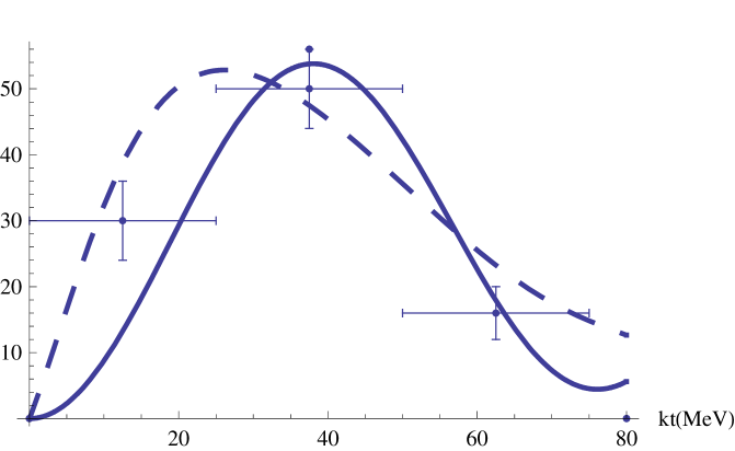
Figure 1: The differential crossection $\frac{d\sigma}{dyd^{2}k_{\perp}}$for y=0 calculated in ADS as a function of transverse meson momentum $k_{\perp}$ (solid line) compared against the photon-pomeron fusion calculation of Hencken et al (dashed line)[16]. . The vertical scale is chosen arbitrarily as normalizations cannot be calculated in our model. Also shown are data points from the Star Collaboration[12] for the number of $\rho^{0}$ counts, binned in 25 MeV intervals.

In fig.1 the crossection, arbitrarily normalized, is plotted for $\rho^{0}$ production in Au-Au UPCs as a function of transverse momentum for $y=0$ and compared against an existing calculation based on photon-pomeron fusion [16]. Also shown are data points from the Star Collaboration[12] for the number of $\rho^{0}$ counts, binned in 25 MeV intervals. Since $g$ is not known, absolute magnitudes cannot be predicted in the ADS model. However, the shape of the momentum distribution is not dissimilar from either experiment or conventional theory. The interference term is crucial, as was found earlier in ref [16].

In summary, we have calculated the quantum fluctuations induced in the 5-D bulk when a point source coupled to vector fields in 4-D space-time is transported along a classical trajectory. The quantum fluctuations amount to the production of different mesons with different momenta in 4-D. Meson crossections are calculable as a function of the point source’s motion. In principle, the motion of a heavy nucleus in an accelerator could lead to the emission of massive particles similar to photon bremsstrahlung but, in practice, the rate is extremely small unless the nuclei have extremely large gamma-factors. On the other hand, for the ultraperipheral collisions of heavy ions, the rates are appreciable. The ADS formalism allows for the prediction of the transverse momentum spectrum. The comparison with existing conventional calculations is fairly satisfactory, and broad features of the existing data are reproduced reasonably well. Emission rates for various excited meson states can be predicted with no additional parameters.

Acknowledgments

The author thanks Tom Cohen for many enjoyable conversations and for sharing critical insights. He would also like to thank other members of the TQHN group at the University of Maryland, particularly Xiangdong Ji and Steve Wallace, for gracious hospitality during a visit made in July 2008 when part of this work was done.

References

• [1] J. Maldacena, β€œThe Large N limit of superconformal field theories and supergravity”, Adv.Theor. Math. Phys. 2:231, 1998, hep-th/9711200; E. Witten, β€œAnti-de Sitter space and holography”, Adv. Theor. Math. Phys.2: 253, 1998, hep-th/9805028; L. Susskind and E. Witten, β€œThe Holographic Bound in Anti-de Sitter Space”, hep-th/9805114
• [2] J. Polchinski and M. Strassler, ”Hard scattering and gauge- string duality”. Phys.Rev.Lett.88:031601,2002, hep-th/0109174; J. Polchinski and M. Strassler, JHEP 0305:012,2003, hep-th/020921; S. J. Brodsky and G. F. de Teramond, ”Light-front hadron dynamics and AdS/CFT correspondence,” Phys. Lett. B 582, 211 (2004) [arXiv:hep-th/0310227].
• [3] H. Boschi-Filho and N. R. F. Braga, ”Gauge string duality and scalar glueball mass ratios,” JHEP 0305, 009 (2003) [arXiv:hep-th/0212207]; S.J.Brodsky and and G.F.de Teramond, ”Hadronic spectra and light-front wavefunctions in holographic QCD”, Phys.Rev.Lett.96:201601,2006, e-Print: hep-ph/0602252.
• [4] J. Erlich, E. Katz, D. T. Son and M. A. Stephanov, ”QCD and a holographic model of hadrons,” Phys.Rev.Lett. 95, 261602 (2005) [arXiv:hep-ph/0501128].
• [5] S. Hong, S. Yoon and M. J. Strassler, ”On the couplings of vector mesons in AdS/QCD,” JHEP 0604, 003 (2006) [arXiv:hep-th/0409118]; ”On the couplings of the rho meson in AdS/QCD,” hep-ph/0501197.
• [6] H. J. Kwee and R. F. Lebed, ”Pion Form Factors in Holographic QCD,” JHEP 0801, 027 (2008) [arXiv:0708.4054[hep-ph]]; S.J.Brodsky and and G.F.de Teramond, ”Light-Front Dynamics and AdS/QCD Correspondence: Gravitational Form Factors of Composite Hadrons”, Phys.Rev.D78:025032,2008, arXiv:0804.0452 [hep-ph]; H. R. Grigoryan and A. V. Radyushkin, ”Pion Form Factor in Chiral Limit of Hard-Wall AdS/QCD Model,” Phys. Rev. D 76, 115007 (2007) [arXiv:0709.0500 [hepph]]; H. R. Grigoryan and A. V. Radyushkin, ”Form Factors and Wave Functions of Vector Mesons in Holographic QCD,” Phys. Lett. B 650, 421 (2007) [arXiv:hep-ph 0703069]. H. J. Kwee and R. F. Lebed, β€œPion Form Factors in Holographic QCD,” arXiv:0708.4054 [hep-ph]; D. Rodriguez-Gomez and J. Ward, β€œElectromagnetic form factors from the fifth dimension,” arXiv:0803.3475 [hep-th].
• [7] Z.Abidin and C.Carlson, ”Gravitational form factors of vector mesons in an AdS/QCD model”, Phys.Rev.D77:095007,2008, hep-ph 08013839
• [8] T. Hambye, B. Hassanain, J. March-Russell and M. Schvellinger, ”On the Delta(I) = 1/2 rule in holographic QCD,” Phys. Rev. D 74, 026003 (2006) [hep-ph/0512089]; ”Four-point functions and kaon decays in a minimal AdS/QCD model,” Phys. Rev. D76, 125017 (2007) [hep-ph/0612010].
• [9] T.Cohen, ”Challenges facing holographic models of QCD”, arXiv:hep-ph 08054813.
• [10] H. Boschi-Filho and N.Braga, ”Bulk versus boundary quantum states”, Phys.Lett.B525:164-168,2002, e-Print: hep-th/0106108.
• [11] C.Itzykson and J.Zuber, ”Quantum Field Theory”, McGraw-Hill International Book Co. (1980)
• [12] Abelev et al, ”$\rho^{0}$ Photoproduction in Ultra-Peripheral Relativistic Heavy Ion Collisions with STAR.”, Star Collaboration, Phys.Rev.C77:34910,2008. E-Print: arXiv:0712.3320
• [13] C.A. Bertulani, S.R. Klein, J.Nystrand, ”Physics of ultra-peripheral nuclear collisions.”, Ann.Rev.Nucl.Part.Sci.55:271-310,2005, E-Print: nucl-ex/0502005. Β
• [14] K.Hencken, ”The Physics of Ultraperipheral Collisions at the LHC”, Phys.Rept.458:1-171,2008, e-Print: arXiv:0706.3356
• [15] J.D.Jackson, Classical Electrodynamics, second edition, John Wiley 1975.
• [16] K. Hencken, G. Baur, D. Trautmann, ”Transverse momentum distribution of vector mesons produced in ultraperipheral relativistic heavy ion collisions”, Phys.Rev.Lett.96:012303,2006, e-Print: hep-ph/0506014.