Dark Matter Gravitational Clustering With a Long-Range Scalar Interaction

Abstract

We explore the possibility improving the $\Lambda$CDM model at megaparsec scales by introducing a scalar interaction that increases the mutual gravitational attraction of dark matter particles. Using N-body simulations, we study the spatial distribution of dark matter particles and halos. We measure the effect of modifications in the Newton’s gravity on properties of the two-point correlation function, the dark matter power spectrum, the cumulative halo mass function and density probability distribution functions. The results look promising: the scalar interactions produce desirable features at megaparsec scales without spoiling the $\Lambda$CDM successes at larger scales.

I Introduction

In this paper we study cosmological implications of a scalar interaction that produces a long-range fifth force in the dark sector, proposed by G. Farrar , S. Gubser and J. Peebles Farrar and Peebles (2004); Gubser and Peebles (2004a, b); Farrar and Rosen (2007); Brookfield et al. (2008). The physical motivation for this model comes from the string theory Battefeld and Watson (2006).

The cosmological motivation comes from small-scale difficulties of the $\Lambda$CDM model, which successfully passes almost all observational tests (see e.g. Spergel et al. (2007)). Difficulties appear at length scales below few megaparsecs: (1) the $\Lambda$CDM voids are less empty than the real voids; (2) the present accretion rate of intergalactic debris onto thin spiral galaxies poses a problem for current galaxy formation paradigm; (3) merger rates at low redshifts for giant elliptical galaxies suggest violent accretion histories for their haloes at low redshifts which is in contradiction with observations.

The void problem, pointed out by J. Peebles Peebles (2001) is hotly debated in the literature, with arguments supporting his original claim Tikhonov and Klypin (2009, 2008) as well as arguments to the contrary Patiri et al. (2006); Tinker and Conroy (2009).

The late merging problem appears in simulations which shows that accretion onto giant elliptical galaxies at cluster centers continues until z = 0 Gao et al. (2004) while the independence of the color-magnitude relation of SDSS galaxies on their environment Hogg et al. (2004) and the remarkable stability of the color-magnitude relation at z = 0.7 Cassata et al. (2007) is consistent with the picture of giant galaxies as island universes, contrary to $\Lambda$CDM simulations. Likewise, according to J. Peebles, the very existence of large galaxies like the Milky Way, with its spiral structure intact, suggests a lack of major mergers in recent history (see Stewart et al. (2008) for thin disk dominated galaxies survival issues). There is observational evidence that the latest “major invasion” happened to our Galaxy 10-12 Gyr ago Gilmore et al. (2002). There are also arguments to the contrary, claiming that Milky Way-like galaxies survive late merging in N-body simulations Governato et al. (2007).

For an excellent discussion of the observational situation and comparison with the $\Lambda$CDM model, see Refs. Perivolaropoulos (2008); Nusser et al. (2005); Peebles and Ratra (2003), and the references therein.

Theoretical suggestions of Peebles and Gubser were followed by the work of Nusser et al. Nusser et al. (2005), exploring the cosmological implications with N-body simulations. Some preliminary results on similar scalar model were also obtained by Rodríguez-Meza et al. Rodríguez-Meza et al. (2007); Rodríguez-Meza (2008); Cervantes-Cota et al. (2007). The Long-Range Scalar Interaction (LRSI) model started a debate in the literature recently, mainly focused on the weak-equivalence principle violation and it’s impact on dynamic of Milky-Way satellites Keselman et al. (2009); Kesden (2009); Kesden and Kamionkowski (2006).

The work, presented here should be regarded as the next step in this line of research. Like Nusser et al., we study the two-point correlation function and the statistical properties of the mass distribution of the dark matter halos. To our knowledge, for the first time in the literature, we also study the power spectra for a set of scalar field parameters with comoving screening length. Analogous model was analyzed in great detail by Grawdohl & Frieman nearly 20 years ago Gradwohl and Frieman (1992); Frieman and Gradwohl (1991). However, their model assumed a fixed physical screening length, which is a fundamental difference in comparison to our model. We have used more particles in our simulations compared to those used by Nusser et al., and our resolution is better than their resolution; we also consider a wider range of scalar model parameters. As a consequence, we resolve the power spectrum near the screening length characteristic scale. Our results show a clear feature in the power spectrum near a wave number,that is the inverse of the screening length. The extra power seen at higher wavenumbers is generated by the gravitational field, enhanced by the scalar interaction. Nusser et al. could not see a similar feature in their correlation function because the screening lengths they considered were too close to the mean interparticle separation in their simulations. Apart from this important difference, we confirm their results. The scalar field generates lower density in voids. It also shifts structure formation to higher redshifts.

This paper is organized as follows: In section II we introduce the effective gravitational potential and modified force law used as an approximation of the scalar field. In Section III we describe our N-body simulations. Our results are presented in Section IV. A brief summary and discussion appears in Section V.

II Theory

Following Refs. Gubser and Peebles (2004a, b), we consider dark matter (DM) particles as strings. Their dynamics is defined by conventional gravity as well as an additional attractive force, induced by an exchange of a massless scalar. This force is well represented by a Yukawa-like potential with a characteristic screening length dynamically generated by the presence of the light particles coupled to scalar (see Ref. Farrar and Peebles (2004) for details on the dynamical screening mechanism). We consider one species of strings as DM particles. The force between two DM particles, each of mass $m$, arises from the potential

$$\Phi({\bf r})=-\,{Gm\over r}\,\,g(x)\,\,,$$ (1)

with

$$g(x)\,=\,1+\beta\,e^{-x/r_{s}}\,.$$ (2)

Here $G$ is Newton’s constant; ${\bf r}$ and ${\bf x}={\bf r}/a(t)$ are, respectively, the particle separation vector in real space and comoving coordinates; $t$ is the cosmological time; $a$ is the scale factor, normalized to unity at present,

$$a(t_{0})\;=\;1\;.$$ (3)

Here and below the subscript “$0$” denotes the present epoch. The parameter $r_{s}$ is the screening length and $\beta$ is a measure of the relative strength of the scalar interaction compared to conventional gravity. The screening length $r_{s}$ is constant in comoving coordinates because of the dynamical screening mechanism, specific to the class of scalar fields considered here. Accordingly, modified potential gives rise to the modified force law between DM particles. The new appropriate form is

$$F_{DM}=-G{m_{1}\cdot m_{2}\over r^{2}}\left[1+\beta\left(1+{r\over r_{s}}\right)e^{-r\over r_{s}}\right]$$ (4)

We can adopt this modification as a distance dependent correction term to ordinary Newton force law:

$$F_{DM}=F_{Newton}\cdot F_{s}(r,\beta,r_{s}),$$ (5)

where $F_{s}$ characterize deviations from standard gravity:

$$F_{s}(r,\beta,r_{s})=1+\beta\left(1+{r\over r_{s}}\right)e^{-r\over r_{s}}$$ (6)

For $\beta=0$ or $r\gg r_{s}$ we have $F_{s}\rightarrow 1$, thus we recover standard Newtonian force law.

Switching from the discrete particle picture to fluid dynamics, we will now introduce the dark matter density field, given by the expression

$$\rho({\bf x},t)=\left<\rho\right>\,(1+\delta)\,,$$ (7)

where $\left<\rho(t)\right>$ is the ensemble average of the dark matter density at time $t$, and $\delta({\bf x},t)$ describes local deviations from homogeneity. The structure formation is driven only by the spatially fluctuating part of the gravitational potential, $\phi({\bf x},t)$, induced by the density fluctuation field $\delta$,

$${\phi({\bf x})\over G{\left<\rho\right>}a^{2}}\,=\,-\int{d^{3}{\bf x^{\prime}}\delta({\bf x^{\prime}})\over|{\bf x-x^{\prime}}|}g\left(|{\bf x-x^{\prime}}|\right)\,.$$ (8)

The Fourier transform of this equation is

$$\phi_{\bf k}=-{3H_{0}^{2}\Omega_{M}\over 2a}\,{\delta_{\bf k}\over k^{2}}\,\left[1+{\beta\over 1+(kr_{s})^{-2}}\right]\,,$$ (9)

where

$$\phi_{\bf k}\,\equiv\,(2\pi)^{-2/3}\,\int\phi({\bf x})\,e^{-i{\bf k\cdot x}}\,d^{3}{\bf x}$$ (10)

and

$$\delta_{\bf k}\,\equiv\,(2\pi)^{-2/3}\,\int\delta({\bf x})\,e^{-i{\bf k\cdot x}}\,d^{3}{\bf x}$$ (11)

are the Fourier transforms of $\phi({\bf x})$ and $\delta({\bf x})$, respectively; ${\bf k}$ is the comoving wavevector, and the quantities

$$\Omega_{M}\,\equiv\,8\pi G\left<\rho\right>_{0}\,/3H_{0}^{2}$$ (12)

and $H_{0}$ are, respectively, the present values of the dimensionless mean dark matter density and the Hubble parameter. From now on, we will also use the symbols $h$ and $\Omega_{\Lambda}$, denoting the dimensionless $H_{0}$, expressed in units of 100 km s^-1Mpc^-1, and the cosmological constant contribution to the present mean density.

Note that when $\beta=0$ or $x\gg r_{s}$, equations (8) and (9) become identical with conventional gravity Peebles (1980). Indeed, consider the fractional deviation from the Newtonian gravitational potential,

$${\Delta\phi_{\bf k}\over\phi_{\bf k}}\;\equiv\;{\phi_{\bf k}-\phi_{\bf k}^{\rm N}\over\phi_{\bf k}^{\rm N}}\;.$$ (13)

Throughout this paper, the label ’Newton’, and the subscript ’N’ refer to the $\Lambda$CDM cosmology with the conventional Newtonian gravity. Equation (9) gives

$${\Delta\phi_{\bf k}\over\phi_{\bf k}}\;=\;{\beta\over 1+(kr_{s})^{-2}}\;\;\;.$$ (14)

This is the Fourier image of the spatial decline of the Yukawa potential: in the limit $kr_{s}\rightarrow 0$, the above expression vanishes. In the opposite limit, the fractional deviation from Newtonian gravity reaches a finite value,

$$\Delta\phi_{\bf k}/\phi_{\bf k}\rightarrow\beta\quad{\rm for}\;\;kr_{s}\gg 1,$$ (15)

$$\Delta\phi_{\bf k}/\phi_{\bf k}\rightarrow 0\quad{\rm for}\;\;kr_{s}\ll 1\;.$$ (16)

We consider values of $\beta$ of order unity and screening lengths of order of few megaparsecs or smaller. Therefore, we can expect that our model predictions differ from the $\Lambda$CDM cosmology only on scales $\sim 1h^{-1}\,{\rm Mpc}$, while on larger scales these two models are indistinguishable, unlike other modifications of gravity, considered recently, for example the DGP model Dvali et al. (2000), $f(R)$ theories Nojiri and Odintsov (2006) ,modifications of the Newtonian gravity on megaparsec scales Sealfon et al. (2005); Shirata et al. (2005, 2007); Stabenau and Jain (2006) or MONDian cosmological simulations Knebe and Gibson (2004).

Here we study only the distribution of the dynamically dominant dark matter particles. We will study the baryon distribution as well in our future work.

III Simulations

In this section we describe our numerical experiments.

III.1 Initial Conditions

To set up the initial conditions, we have to define the power spectrum of the dark matter density fluctuations,

$$P(k)\,=\,\left<|\delta_{\bf k}|^{2}\right>\,.$$ (17)

We use a power spectrum, derived from the cmbfast code by Seljak & Zaldarriaga Seljak and Zaldarriaga (1996) with cosmological parameters $h=0.7$, $\Omega_{M}=0.3$, $\Omega_{\Lambda}=0.7$ and $\sigma_{8}=0.8$. The last in this set of parameters is the present value of the root-mean-square density contrast of dark matter spatial fluctuations within a 8 ${h^{-1}\,{\rm Mpc}}$ sphere. This is the conventional normalization parameter and a measure of the degree of inhomogeneity of the dark matter distribution.

The resulting power spectrum, together with the PMcode by Klypin & Holtzman Klypin and Holtzman (1997) is used to displace particles from their regular lattice positions, following the Zel’dovich approximation (see Ref. Efstathiou et al. (1985) for details). The number of individual simulations for each set of model parameters has to be large enough to allow a decent average over simulation-to-simulation phase fluctuations. We decided that for our purposes “a large enough number” is 10 realizations for $200h^{-1}\,{\rm Mpc}$ box simulations. In this manner we have obtained an ensemble average of simulations in the large box.

III.2 The codes

We use the freely available codes: (1) AMIGA (Adaptive Mesh Investigations of Galaxy Assembly) by Knebe, Green, Gill & Saar which is the successor of the MLAPM code Knebe et al. (2001) and (2) GADGET2 by Volker Springel Springel et al. (2001); Springel (2005). AMIGA is a Particle Mesh code with implementation of the Adaptive Mesh Refinements(AMR) technique to obtain high force resolution. GDAGET2 is a Tree-Particle Mesh code. We use AMIGA’s pure Particle Mesh (PM) kernel for large box simulation, reducing the simulation time at the expense of the force resolution. For study of the halo clustering properties we used GDAGET2. To accommodate for the poor mass resolution we have divided our simulations into two sets.

The first set of simulations was used to study the power spectrum and the spatial correlation function of the dark matter density fluctuations and density probability distribution functions. The simulation box in this series of simulations has a width $200h^{-1}\,{\rm Mpc}$, allowing proper treatment of the fundamental mode of density perturbations, which remains in the linear regime at redshift $z=0$. These are pure PM simulations.

In the second set of simulations we have used a box of width $25h^{-1}\,{\rm Mpc}$. These simulations are used to study the cumulative halo mass function and the redshift evolution of halo abundances and $p(\delta)$. This approach provides a better force and mass resolution, but due to the smallness of the box we lack some power in large scales. For a discussion of the influence of the box size on the dynamics and statistics of simulations, see Ref. Power and Knebe (2006); Bagla and Ray (2005).

In each experiment we save the particle positions and velocities at redshifts 5; 3; 2; 1; 0.9; 0.8; 0.7; 0.6; 0.5; 0.4; 0.3; 0.2; 0.15; 0.1; 0.05, and the redshift of the final output, $z=0$. This archive is used to study the evolution of the dark matter distribution with redshift. For an experiment, involving $N_{p}$ dark matter particles in a box of size $L$ at present, the particle mass, $m_{p}$, is given by

$$m_{p}\,=\,\left<\rho\right>\,(L^{3}/N_{p}).$$ (18)

For our simulations, $N_{p}=128^{3}$ for 200 $h^{-1}\,{\rm Mpc}$ box and $N_{p}=256^{3}$ for 25 $h^{-1}\,{\rm Mpc}$. The other important simulation parameters are the force resolution $\varepsilon$, the interparticle separation,

$$\ell\;=\;(L^{3}/N_{p})^{1/3}\;\;,$$ (19)

and the Nyquist wavenumber,

$$k_{\rm Nyq}\;=\;\pi/\ell\;\;.$$ (20)

Table 1: Simulation parameters. $L\,$ is the box size $[h^{-1}\,{\rm Mpc}]$; $\,z\,$ is the initial redshift; $\,m_{p}\,$ is the mass of a single particle $[h^{-1}M_{\odot}]$; $\,\varepsilon\,$ is the force resolution $[h^{-1}\,{\rm kpc}]$; $\,\ell\,$ is the mean interparticle separation $[h^{-1}\,{\rm Mpc}]$; $\,k_{\rm Nyq}\,$ is the Nyquist wave number $[h{\rm Mpc}^{-1}]$; $\,r_{s}\,$ is the screening length $[h^{-1}\,{\rm Mpc}]$; and $\,\beta\,$ is the relative strength of the scalar force.

$L$	$\;z$	$m_{p}$	$\varepsilon$	$\ell$	$k_{\rm Nyq}$	$r_{s}$	$\beta$
200	30	$3.18\cdot 10^{11}$	800	1.563	2.01	$1;2;5$	$-0.5;0;0.2;0.5;0.7;1$
25	60	$7.7\cdot 10^{7}$	10	0.097	32.1	$0.5;1;1.5;2$	$0;0.2;0.5;1$

We list the above parameters, evaluated for the large and the small box, in Table 1.

III.3 The Green’s Function

For conventional gravity in Fourier space, the discrete Poisson equation can be written as

$$\phi_{\bf k}\,=\,{3H_{0}^{2}\Omega_{M}\over 2a}\,\delta_{\bf k}\,{\mathcal{G}}_{\bf k}\,,$$ (21)

where ${\mathcal{G}}_{\bf k}$ is the Green’s function. We use the seven-point finite-difference approximation to the Green’s function to solve the Poisson’s equation in a cubic box with periodic boundary conditions. It is defined for a discrete set of arguments,

$${\bf q}\,=\,\{q_{j}\}\,=\,{\bf k}\cdot L/(2\pi)\,,$$ (22)

where $L$ is the present size of the comoving simulation box. The subscripts $j=1,2$, or $3$ denote the three dimensions in ${\bf k}$ space. The number of grid cells in each dimension is ${\mathcal{N}}$ (256 in our simulations), so the cell numbers assume integer values in the range

$$q_{j}\,=\,1,2,\,\ldots\,,{\mathcal{N}}\,.$$ (23)

Each integer triple defines the grid point, at which the Green’s function is evaluated:

$${\mathcal{G}}_{\bf q}^{\rm N}=-\pi\left[{\mathcal{N}}^{2}\sum_{j=1}^{3}\sin^{2}(\pi q_{j}/{\mathcal{N}})\right]^{-1}\,.$$ (24)

Using the equation. (9), we modify Green’s function to get the proper potential for our model of scalar interactions:

$${\mathcal{G}}_{\bf k}^{\rm scalar}={\mathcal{G}}_{\bf k}^{\rm N}\,\,\left(1+{\beta\over 1+(kr_{s})^{-2}}\right)\,\,.$$ (25)

The AMIGA code and PM part of the GADGET2 code uses equation (21) and the fast Fourier transform technique to evaluate the gravitational potential at grid points. GADGET2 use Oct-Tree algorithm to calculate short distance part of the particle forces, we have modified this part of the code using equations (5,6) accordingly. Then particle positions and momenta are updated in the standard way for N-body algorithms.

III.4 Particles and Halos

To identify collapsed objects from now on called ’halos’ we have used AMIGA’s Halo Finder (AHF) by Knollman & Knebe Knollmann and Knebe (2009) which is the successor of the MHF halo finder by Gill, Knebe & Gibson Gill et al. (2004). The AHF uses AMR to find halo centers, then it probes the halo density profile around each center in nested radial bins until the spatially averaged density contrast reaches the virial overdensity, $\,\Delta$. At $z=0$, in a $\Lambda$CDM universe Gross (1997), $\,\Delta=340$. Given our mass resolution in the bigger box, we can expect to follow the assembly of halos, corresponding to clusters and superclusters, and study the statistics of clustering at large scales. Simulations in the small box should be good enough to investigate the assembly of much less massive objects, like halos of clusters and galaxies.

It is important to bear in mind that at small scales we are limited by force resolution. The smallest size of gravitationally bound objects that can form in our box is $2\varepsilon$ (see Table 1 and Ref. Knebe et al. (2000)). We also suffer from the well-known problem of overmerging described in great detail by Klypin et al. in Ref. Klypin et al. (1999). As a consequence, our simulations underestimate low-mass object abundances.

IV Results

In this section we present the results obtained in our numerical experiments. We provide maps of the spatial distribution of dark matter particles as well as clumps of particles, called halos. We also study different statistical measures of clustering, such as the power spectrum, the two-point correlation function, density probability distribution function, and the cumulative halo mass function with and without the scalar interaction.

Figure 1: Slices cut through centers of simulation boxes of width $200h^{-1}\,{\rm Mpc}$ at $z=0$. The plots show particle positions, ${\bf x}$, in the $(x_{1},x_{2})$ plane. Each slice has dimensions $200\times 200(h^{-1}\,{\rm Mpc})^{2}$ in this plane and a thickness of $10h^{-1}\,{\rm Mpc}$ along the $x_{3}$ coordinate axis.

IV.1 The Clustering Pattern

Figure 1 shows the final particle distribution in $10h^{-1}\,{\rm Mpc}$ slices, cut through the centers of $200h^{-1}\,{\rm Mpc}$ simulation boxes. For clarity each slice shows only 1/10 of the total number of particles, selected at random

The frame, labeled ’$\Lambda{\rm CDM}$’ in Figure 1 assumes $\beta=0$, while the remaining frames show particle distributions for a set of different $\beta$ parameters and a fixed screening length, $r_{s}=2h^{-1}\,{\rm Mpc}$. As a test, we also consider ’antigravity’ with $\beta=-0.5$. All of the frames in Figure 1 have evolved from the same initial state, with identical amplitudes and phases of density fluctuations, set up at $z=30$.

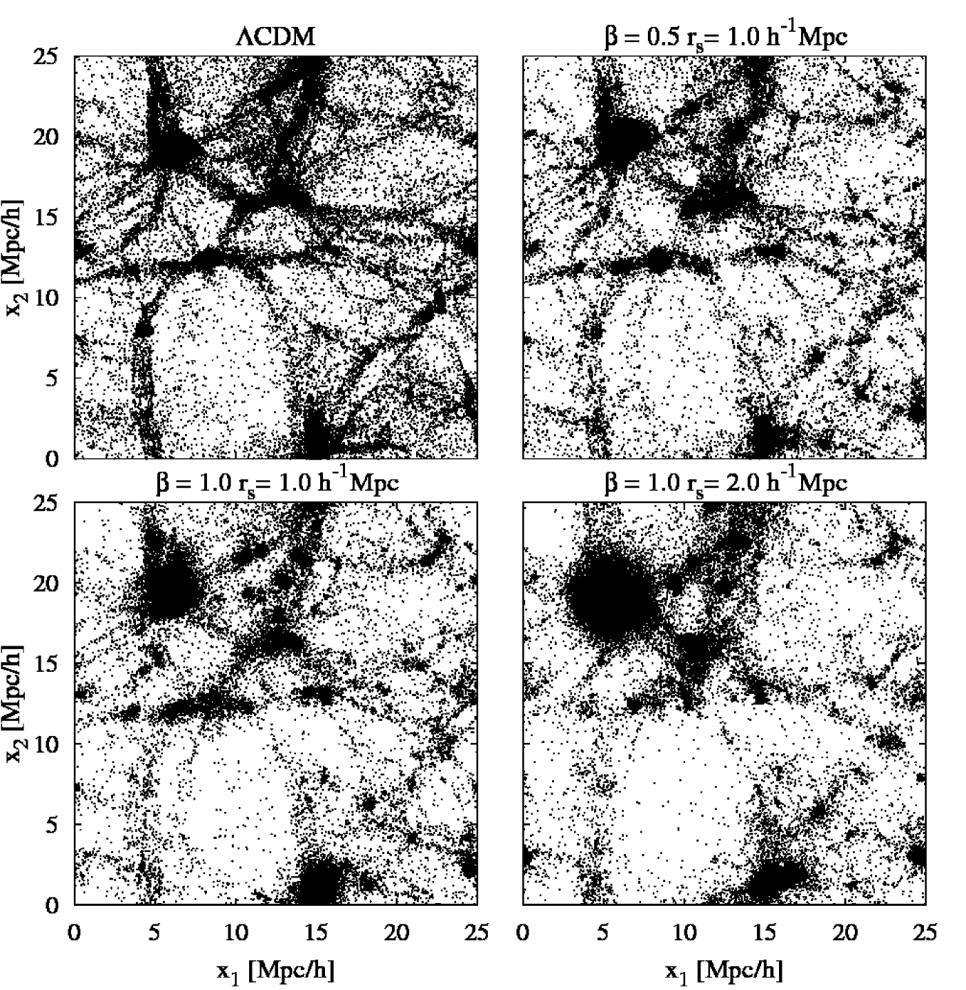
Figure 2: Similar results for the smaller box, $L=25h^{-1}\,{\rm Mpc}$. The thickness of each slice is $1.5h^{-1}\,{\rm Mpc}$.

At first sight, modified gravity simulations look similar to the $\Lambda{\rm CDM}$ case. The filaments, voids and high-density peaks occupy similar positions in the frames. However, close inspection shows that with increasing $\beta$, the voids appear increasingly more empty. This phenomenon is seen more clearly in Figure 2, where we show $1.5h^{-1}\,{\rm Mpc}$ slices, cut through the centers of our smaller simulation boxes ($L=25h^{-1}\,{\rm Mpc}$).

Figure 2 also shows that the scalar forces enhance the accretion of matter, producing more massive halos at small scales. Pancake-like structures, seen in the $\beta=0$ frame, are more homogeneous than their counterparts in frames with $\beta>0$, which show substructure. The fragmentation into subsystems of smaller halos is increasingly more pronounced, with increasing values of $\beta$. Quantitatively, we can expect an increase of the amplitude of the power spectrum at small scales, corresponding to wave numbers $k\gtrsim r_{s}^{-1}$, and an opposite effect for $\beta=-0.5$, when the pancakes appear even more homogeneous than those generated by Newtonian gravity.

IV.2 The Power Spectrum

The power spectrum is a convenient measure of the strength of dark matter clustering. It is well constrained by redshift surveys of galaxies, such as the SDSS catalog. In the longwave tail, corresponding to wave numbers

$$0.01\,{\rm Mpc}^{-1}h\;\leq k\;\leq\;0.3\,{\rm Mpc}^{-1}h\;\;,$$ (26)

this survey provides a reliable estimate of $P(k)$ Tegmark et al. (2006). In this range, the $\Lambda$CDM power spectrum agrees well with observations. We also use non-inear fit to the power spectrum presented by Smith et al. in Smith et al. (2003) as a measure of theoretical $\Lambda{\rm CDM}$ P(k). This can be used to constrain scalar field models.

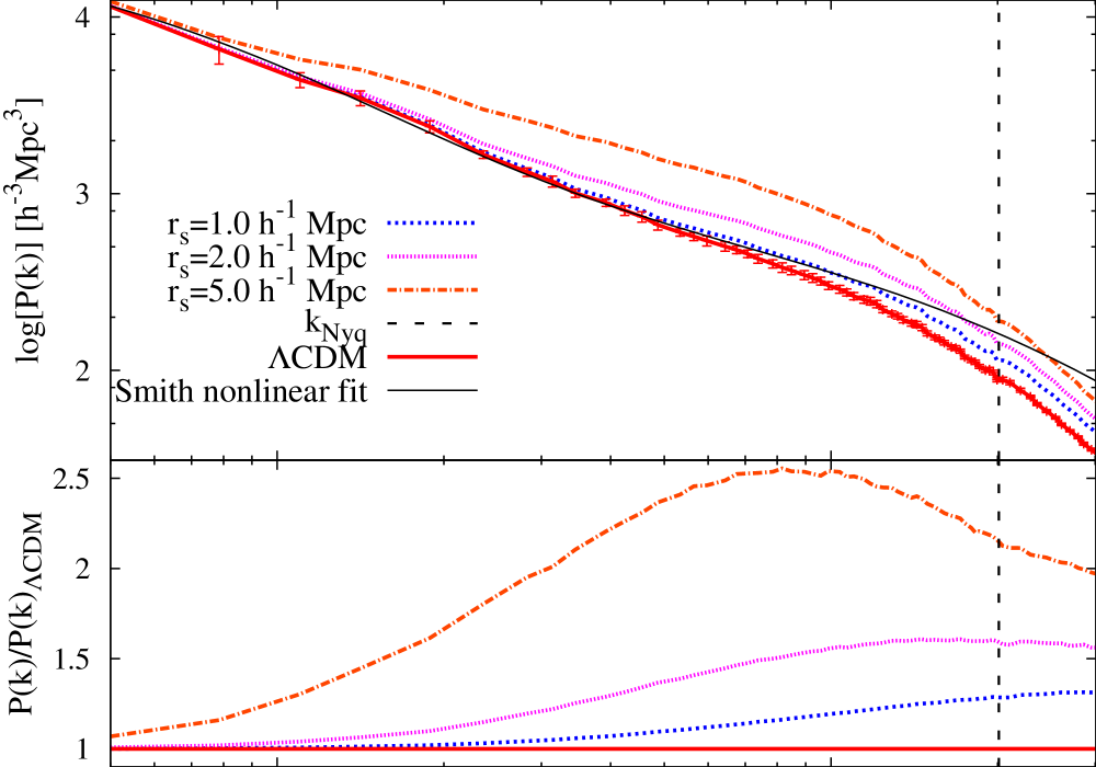
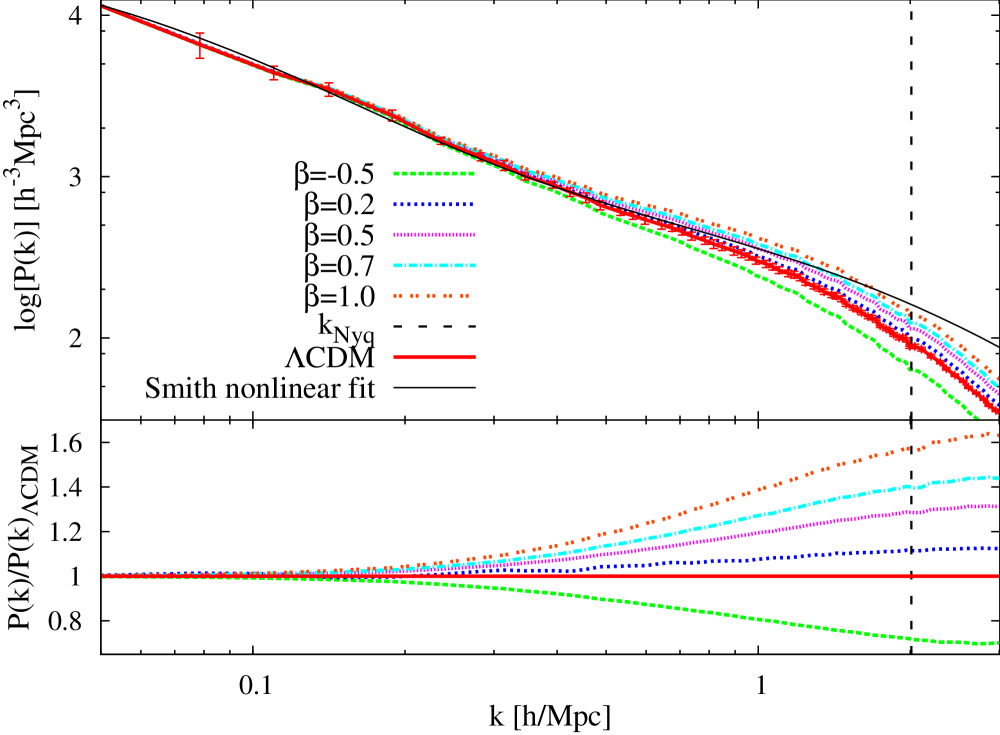
Figure 3: Power spectra from simulations with $L=200h^{-1}\,{\rm Mpc}$. Vertical dashed lines show the Nyquist wave number, while the thin black line is the nonlinear fit for $\Lambda{\rm CDM}$ $P(k)$ from Smith et al. We also plot the ratio of the scalar interaction induced $P(k)$ to its Newtonian counterpart, $P_{\rm N}(k)$. For all of the upper pair of plots $\,\beta=1$, while the $\,r_{s}\,$ parameter is allowed to vary. For the bottom pair $\,r_{s}=1h^{-1}\,{\rm Mpc}\,$ is fixed, while the value of $\,\beta\,$ changes from $\,-0.5\,$ to $\,1$. Each curve was obtained by averaging over 10 realizations with different initial phases.

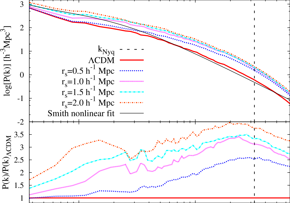
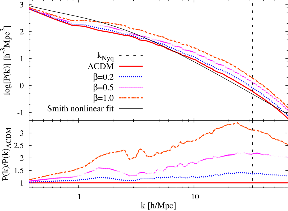
Figure 4: Power spectra plots similar to those in figure 3, obtained from a set of simulations, using the smaller box, $L=25h^{-1}\,{\rm Mpc}$.

In Figure 3 we plot the final power spectra, obtained from the simulations with $L=200h^{-1}\,{\rm Mpc}$. The top pair of plots shows $P(k)$ and the ratio $P/P_{\rm N}$ for scalar forces with fixed $\beta=0.5$ and a varying screening length. The pair of plots below was obtained from simulations with a fixed screening length, $r_{s}=1h^{-1}\,{\rm Mpc}$, and a varying $\beta$.

These plots show that the rate of growth of density perturbations is more sensitive to the range of the scalar field, $r_{s}$, than to its strength, as long as $\beta>0$. The scalar force increases the rate of growth of density fluctuations on comoving scales, smaller than $r_{s}$ and wave numbers $k\gtrsim r_{s}^{-1}$. As expected, there is an opposite effect for $\beta=-0.5$: the rate of growth of density perturbations at small scales is reduced.

We describe the deviations from the Newtonian power spectrum at a given wave number by the parameter

$${\Delta P\over P}\,\equiv\,{P-P_{\rm N}\over P_{\rm N}}\;\;\;.$$ (27)

These deviations remain negligible on large scales for all of the considered models with one exception: the model with $r_{s}=5h^{-1}\,{\rm Mpc}$. For this model, $\Delta P/P$ is significant on all scales present in the simulation box, including the SDSS wave number range. Therefore all scalar field models with $r_{s}\geq 5h^{-1}\,{\rm Mpc}$ do not appear promising. To assign statistical significance to their failure to reproduce the real Universe, it is necessary to create a mock SDSS survey and reproduce the power spectrum estimator, used by the observers. We are planning to run appropriate Monte Carlo simulations and address this problem in greater detail in a forthcoming paper.

The model with $\,r_{s}=5h^{-1}\,{\rm Mpc}\,$ may not be successful in reproducing the real Universe, but it is extremely useful in understanding the physics of the scalar field because this value of the screening length is much larger than the interparticle separation in the big box, $\,\ell\approx 1.6h^{-1}\,{\rm Mpc}$. Therefore, we can resolve the difference between purely Newtonian gravity and the scalar field. Indeed, for $\,k=1/r_{s}=0.2\,$, and $\,\beta=0.5\,$, we get $\,\Delta P/P=0.5\,$ (see Figure 3), and an increasing $\,\Delta P/P\,$ for larger wave numbers. The gravitational attraction, enhanced by the scalar field generates the extra power in the plot. To look for a similar jump in amplitude for smaller values of $\,r_{s}\,$, we need a better resolution. So, we have to turn to the simulations in the smaller box, where $\,\ell=125h^{-1}\,{\rm kpc}$. And we do find a similar feature: for $\,\beta=0.5\,$ and $\,r_{s}=1h^{-1}\,{\rm Mpc}\,$, we get $\,\Delta P/P=0.5\,$ at $\,k=1/r_{s}=1h{\rm Mpc}^{-1}\,$ (see Figure 4)!

The decline of $P_{\rm N}/P$ with decreasing wave number in all considered models is a natural consequence of the presence of the Yukawa cutoff, reflected in the equation (14).

In the opposite limit, with growing wave numbers, all power spectra in Figure 3 seem to misbehave. Equation (16) suggests that all $P_{\rm N}/P$ curves should flatten for large wave numbers, $\,k\gg 1/r_{s}$. Instead, we see a decline. Since this behavior is in disagreement with gravitational dynamics, and since it appears in the range $k\gtrsim k_{\rm Nyq}$, we can expect that the decline is an artifact of the discrete nature of the simulation. If this is indeed the case, then in the simulation in the smaller box, this artifact should move to higher wave numbers. This simulation has a smaller interparticle separation and a better force resolution. Hence, for wave numbers in the range

$$r_{s}^{-1}\;\lesssim\;k\;\lesssim\;k_{\rm Nyq}\;\;,$$ (28)

we should see a flat section of the $P/P_{\rm N}$ curve, followed by a decline for $k\gtrsim k_{\rm Nyq}\;$. This is exactly what happens in Figure 4. The $P_{\rm N}/P$ ratio rises with $k$ until it reaches its maximum, followed by a plateau, and then decline for wave numbers above the Nyquist limit.

IV.3 The Correlation Function

Another convenient measure of the strength of clustering is the spatial two-point correlation function,

$$\xi\,\left(|{\bf x-x^{\prime}}|,\,t\right)\;=\;\left\langle\,\delta({\bf x},t)\delta({\bf x^{\prime}},t)\,\right\rangle\;.$$ (29)

It is related to the power spectrum by the Fourier transform,

$$\xi\,(x)\;=\;(2\pi)^{-3}\,\int\,P(k)\,e^{i{\bf k\cdot x}}\,d^{3}{\bf k}\;.$$ (30)

Under ideal conditions, when the power spectrum is determined in the entire wave number range from zero to infinity, $P$ and $\xi$ are equivalent to each other. However, measurements from simulations or galaxy redshift surveys provide only noisy estimates of $P(k)$ or $\xi(x)$ for limited ranges of $k$ and $x$. Therefore, in numerical experiments, it is safer to estimate $\xi(x)$ directly from the particle positions in the simulation output, using the expression (29), or its discrete version, based on the probability density of finding a pair of particles in a separation range from $x$ to $x+dx$ (see Ref. Peebles (1980)). The results presented in this section are therefore not a mere Fourier transform of the results discussed in the two previous subsections. Following the approach we used to study power spectrum deviations from the Newtonian case, here we introduce a similar measure of the deviations of the scalar-induced correlation function from its Newtonian cousin, $\xi_{\rm N}$. This is the quantity

$$\dfrac{\Delta\xi}{\xi}\;\;\equiv\;\;\dfrac{\xi-\xi_{\rm N}}{\xi_{\rm N}}\;.$$ (31)

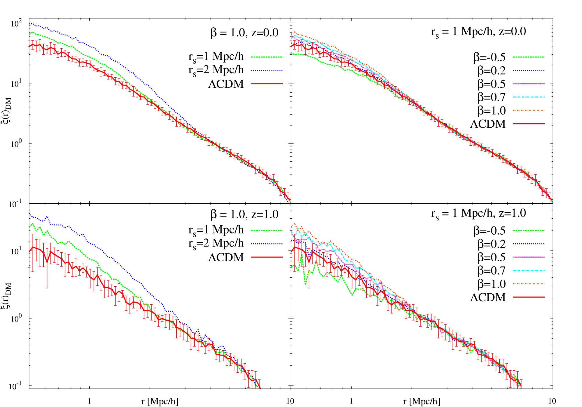
Figure 5: The correlation function for pairs of DM particles at redshift z = 1 (bottom frames) and z = 0 (top frames). The width of the simulation box is $200h^{-1}\,{\rm Mpc}$. All plots were averaged over 10 simulations. To avoid overcrowding, we show 1 standard deviation error bars for the Newtonian $\,\xi(x)\,$ only. The error bars for the scalar-induced correlation functions are similar. Their size is determined mostly by the number of realizations and by the size of the box. Both these quantities are identical for all simulations presented here.

The four frames in Figure 5 show two-point correlation functions for DM particles in the $200h^{-1}\,{\rm Mpc}$ box. The top two frames show simulation outputs at $z=0$, while the bottom frames refer to an earlier epoch, $z=1$. For clarity, we show one standard deviation errors only for the Newtonian case. The error bars for the remaining models are similar.

The large amplitude in $\,\Delta\xi/\xi\,$ at separations $\,x\lesssim 1h^{-1}\,{\rm Mpc}$ is probably an artifact because the separations involved are smaller than $\,\ell=1.56h^{-1}\,{\rm Mpc}$. Nusser et al. Nusser et al. (2005) have discovered a similar shoulder in $\,\xi(x)\,$ in their simulations and they provided an interpretation similar to ours. They have also pointed out that the correlation function in their simulations does not possess a feature at $\,x=r_{s}\,$ “despite the scalar force attraction at smaller scales.“ We believe that the source of this problem is poor resolution, not dynamics. The range of screening lengths they consider is uncomfortably close to their interparticle separation. Our correlation functions, plotted in Figure 5, suffer from the same problem. As we have shown in our discussion of the properties of simulated power spectra, this problem can be avoided by improving the resolution. For an appropriate choice of the box size and the screening length, when $\,r_{s}>1/k_{\rm Nyq}\,$, the feature at $\,k=1/r_{s}\,$ can be resolved. We therefore have no doubt - the feature is there. To rediscover for $\,\xi(x)\,$ what we have already seen for $\,P(k)\,$, we only need higher resolution simulations, like those in Ref.Springel et al. (2005), but with a modified Green’s function.

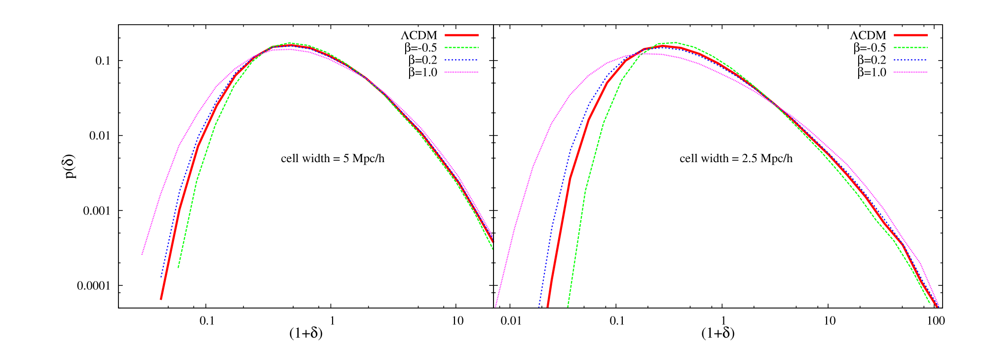
Figure 6: The density probability distribution functions obtained from $200h^{-1}\,{\rm Mpc}$ boxes. Results for fixed $r_{s}=1h^{-1}\,{\rm Mpc}$. Left panel shows $p(\delta)$ calculated using the grid cells width of $5h^{-1}\,{\rm Mpc}$, while in the right panel are functions calclated with cells width of $2.5h^{-1}\,{\rm Mpc}$.

Despite the modest resolution of the present results, we believe that qualitatively, the stratification of the correlation functions with respect to $r_{s}$ and $\beta$, seen in Figure 5 reflect the true dynamics. Note that for $\,\beta<0\,$, when gravity is weaker than Newtonian, we get $\,\Delta\xi/\xi\ <0\,$, which is dynamically reasonable.

Our results also differ from those of Nusser et al. at larger separations, $x>3h^{-1}\,{\rm Mpc}$, where according to their Figure 7, $\,\Delta\xi/\xi<0$. This does not happen in our simulations unless $\beta<0$. This discrepancy, however, becomes statistically insignificant if we use our error bars for guidance (Nusser et al. do not provide error bars for their plots).

As we have already mentioned, for separations $x>r_{s}$, $\Delta\xi/\xi$ is consistent with zero for all models considered here. This is good news, since the observed $\xi(x)$ at large separations agrees well with the $\Lambda$CDM model.

Last but not least, it is worth noticing that in Figure 5, $\Delta\xi/\xi$ is higher at $z=1$ than at $z=0$. The growth of Newtonian $\xi$ is retarded with respect to the scalar-induced $\xi$ at high redshift. Later, $\xi_{\rm N}$ ’catches up’ with the scalar $\xi$. As a consequence, $\Delta\xi/\xi$ is reduced. A possible explanation for this phenomenon is that in the presence of scalar forces, rapid matter accretion and formation of virialized objects occurs at earlier epochs than in the standard gravity model. This interpretation is supported by our direct analysis of the process of halo formation, presented below.

IV.4 Emptiness of the voids

As a measure of the emptiness of the voids in our simulations we will use the density contrast probability distribution function $p(\delta)$. To calculate these functions we extrapolate particle positions to the uniform lattice grid to obtain density. After conversion to the density contrast we compute $p(\delta)$ numerically in the usual way, by using

$$dp(d\delta)={\sum_{i}^{N_{c}}[\delta_{Dirac}(\delta_{i}=d\delta)]\over N_{c}}\;\;\;,$$ (32)

where the sum runs for all the cells, and $N_{c}$ is the total number of cells and $\delta_{i}$ is a density contrast in a $i$-th cell. We have calculated the density contrast probability distribution function for the large and small boxes. The results are presented in figures 6 and 7.

In Figure 6 we show $p(\delta)$ calculated in the $200h^{-1}\,{\rm Mpc}$ box. Functions in the left frame was calculated using the $5h^{-1}\,{\rm Mpc}$ grid cell width, while on the right frame we show density probability distribution functions obtained with the $2.5h^{-1}\,{\rm Mpc}$ grid cell width. In both cases we show the effect of varying the $\beta$ parameter keeping the screening length $r_{s}=1h^{-1}\,{\rm Mpc}$. In Figure 7 we plot probability distribution functions (PDFs) oobtained from simulations in the small box. The density field was calculated on a uniform grid of cells with length of $1h^{-1}Mpc$. On the left frame we show functions in models with fixed $r_{s}=1h^{-1}\,{\rm Mpc}$ and varying $\beta$. In the right frame we plot the results for models with fixed $\beta=1$ and various $r_{s}$ values.

Clearly we see, that introduction of LRSI stretches the $p(\delta)$ toward a smaller density contrast, while keeping the relative value at high density tail close to the $\Lambda{\rm CDM}$ case. This is striking confirmation of what was expected. LRSI produce emptier voids. The smaller the considered cell width the more pronounced the effect. An interesting effect seen in our distribution functions is the reduced skewness. This is different from standard gravity which increases the skewness Juszkiewicz et al. (1993). We will study this effect in the future.

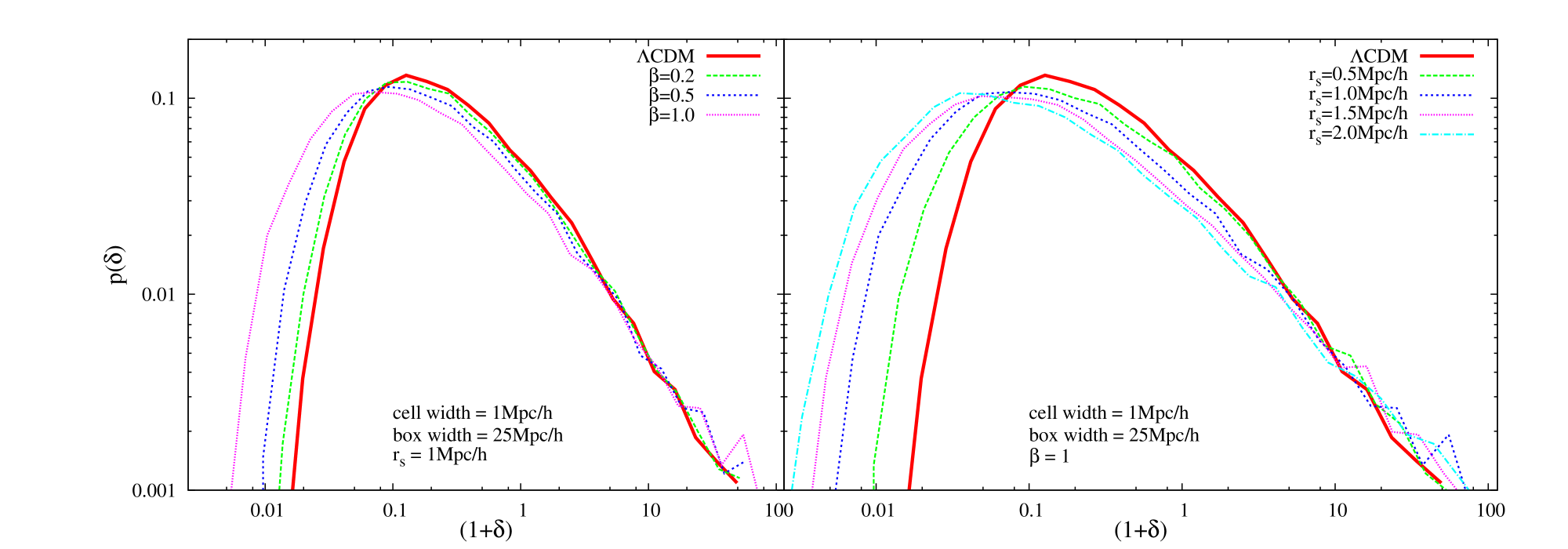
Figure 7: This figure is analogous tho the previous one. Here we present the $p(\delta)$ obtained from $25h^{-1}\,{\rm Mpc}$ boxes. The cell width used for calculation was $1h^{-1}\,{\rm Mpc}$. LRSI models in the left panel have fixed $r_{s}=1h^{-1}\,{\rm Mpc}$, on the right panles $r_{s}$ vary and we keep $\beta=1$ fixed.

IV.5 Halos formation in the Small Box

Figure 8: Positions of halo centers obtained from a particular simulation output. The size of the box is $\,L=25h^{-1}\,{\rm Mpc}$. To avoid overcrowding, we show only the halos with centers in the range $\,0\leq x_{3}\leq 5h^{-1}\,{\rm Mpc}$. Halos with masses greater than $\,5\cdot 10^{12}M_{\odot}\,$ appear as circles. Their diameters are proportional to their masses. Less massive halos are represented by dots. The top left frame shows the standard gravity case. The halo distribution in all of the remaining frames is plotted for $\,r_{s}=1h^{-1}\,{\rm Mpc}\,$ and three different values of $\,\beta$. The circle above the upper frame represents a halo with a mass of $\,2\cdot 10^{13}M_{\odot}$.

Figure 9: Maps of the halo distribution, derived from the same simulations as those shown in Figure 8, but for halos with masses, smaller than ${\tt M}=2\cdot 10^{10}h^{-1}M_{\odot}$. Even smaller halos with masses $\,M\leq{\tt m}=8\cdot 10^{9}h^{-1}M_{\odot}$ are represented by dots. Those with masses in the range $\,{\tt m}<M\leq{\tt M}\,$ appear as circles.

In this section we study the impact of modified gravity on the halo formation process. To identify halos, we apply the halo finder program (the AHF, introduced earlier) to output snapshots from the $25h^{-1}\,{\rm Mpc}$ simulations. We study all halos with more than 20 particles, hence our minimal halo mass is $1.5\cdot 10^{9}h^{-1}M_{\odot}$.

IV.5.1 High Mass Halos

In Figure 8 we plot the present comoving positions ${\bf x}=(x_{1},x_{2},x_{3})$ of halo centers in the $(x_{1},x_{2})$ coordinate plane of the simulation box. To avoid overcrowding, we consider only halo centers that satisfy the condition $0\,\leq\,x_{3}\,\leq\,5h^{-1}\,{\rm Mpc}$. Halos with masses exceeding $\,{\tt M}=5\cdot 10^{12}h^{-1}M_{\odot}\,$ are plotted as circles with diameters proportional to halo masses. For reference, the size of a circle, representing a halo with a mass of $2\cdot 10^{13}M_{\odot}$ is shown in Figure 8, above the upper left frame. The halos with masses $M<{\tt M}$ are plotted as dots. It is interesting to note that as expected, the scalar interactions enhance the ability of the larger halos to accrete matter and become even larger. This effect is particularly striking when we compare the upper left, Newtonian frame, with the lower right frame where $\,r_{s}=1h^{-1}\,{\rm Mpc}$ and $\,\beta=1$. The halos seen in the rectangle

$$5h^{-1}\,{\rm Mpc}\;<\;x_{1}\;<10h^{-1}\,{\rm Mpc}\;\;,$$ (33)

$$15h^{-1}\,{\rm Mpc}\;<\;x_{2}\;<25h^{-1}\,{\rm Mpc}\;\;,$$ (34)

at lower right have already acreted all debris in their vicinity at earlier times, while in the Newtonian frame the accretion process is still going on. At the same time, the small-scale mass redistribution process does not affect the large scale clustering: the cosmic web is clearly visible in all of the frames.

IV.5.2 Low-mass Halos

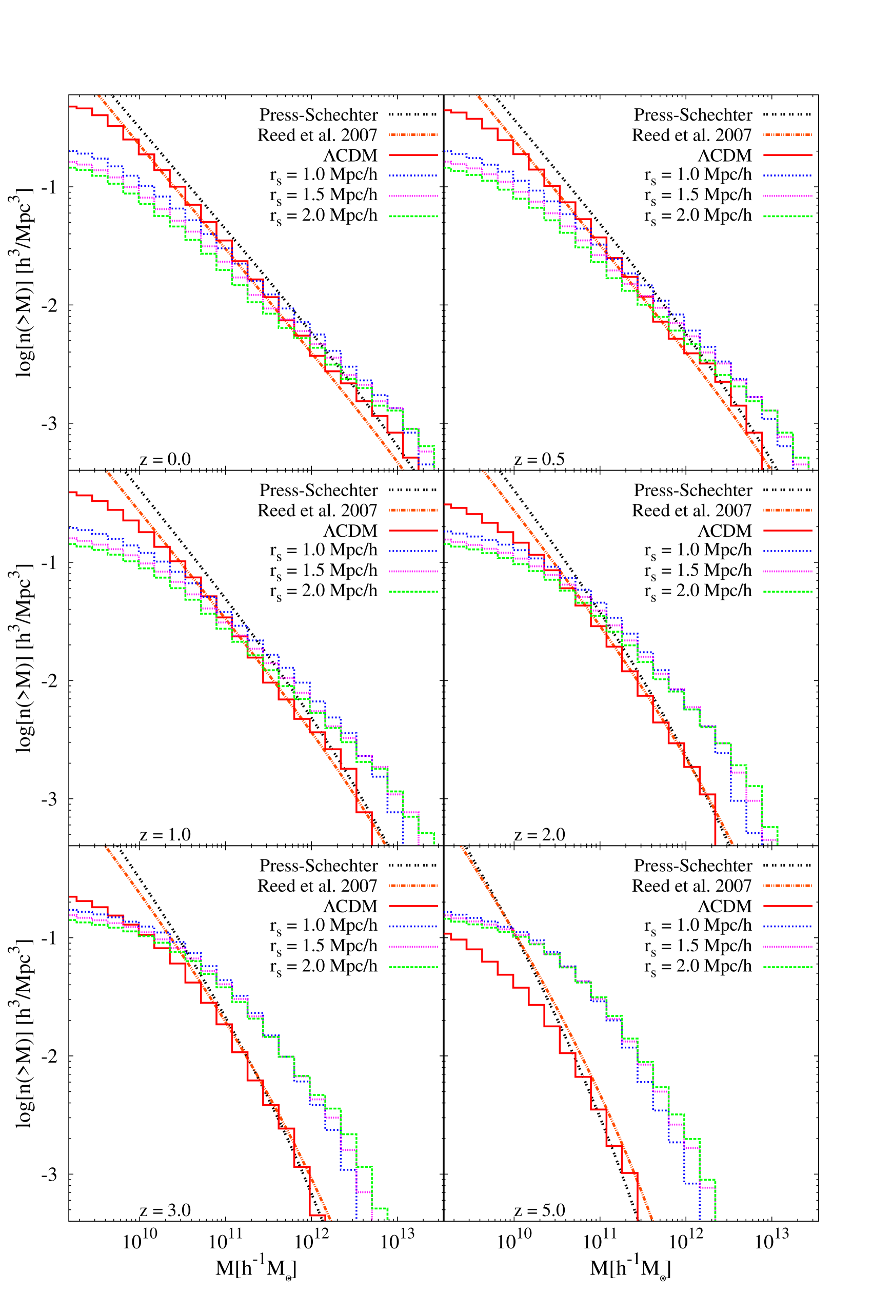
Figure 10: The redshift evolution of the cumulative halo mass functions in simulations with $\,L=25h^{-1}\,{\rm Mpc}\,$. We show the $\Lambda{\rm CDM}$ case and two scalar models with $\,\beta=1\,$ and two different values of $\,r_{s}\,$.

In this section we look at the low-mass end of the halo population. Our Figures 9 and 8 are complementary to each other. Both are derived from the same simulation, except this time we show only halos with masses $\,M\leq{\tt m}=2\cdot 10^{10}h^{-1}M_{\odot}\,$. The circles show halos with masses $\,8\cdot 10^{9}h^{-1}M_{\odot}\leq M\leq{\tt m}$. The remaining halos, with masses $\,M\leq 8\cdot 10^{9}h^{-1}M_{\odot}$, are plotted as dots. As before, the diameters of the circles are proportional to halo masses. The influence of the scalar field is particularly well pronounced when we compare frames with scalar field switched off ($\,\beta=0$, upper left) and on ($\,\beta=1$, lower right). The low abundance of light halos, seen here, is consistent with the high abundance of heavy halos in Figure 8. Both figures show the rapid accretion and massive halo formation at high redshift, induced by the scalar force.

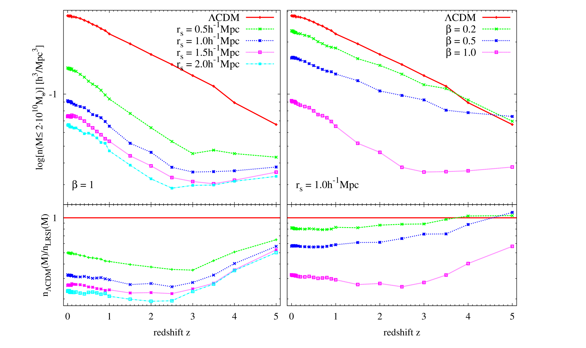
Figure 11: Redshift evolution of the abundance of low-massive halos. Here, we consider only halos with $M\leq 2\cdot 10^{10}h^{-1}M_{\odot}$ The bottom panels show the ratio of the halo abundance to the $\Lambda{\rm CDM}$ case.

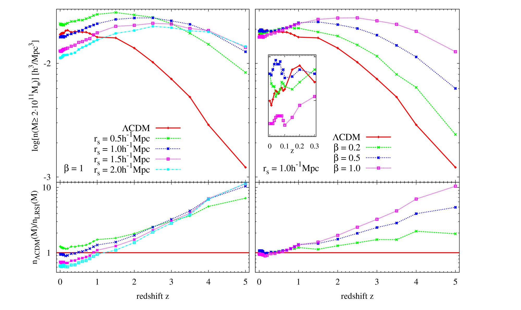
Figure 12: Redshift evolution of the abundance of high-massive halos. Here we consider only halos with $M\geq 2\cdot 10^{11}h^{-1}M_{\odot}$ The bottom panels show the ratio of the halo abundance to the $\Lambda{\rm CDM}$ case. The small box inset in the bottom right frame is a magnification of the $\,0\leq z\leq 0.3\,$ region in the same frame.

IV.5.3 The Cumulative Mass Function

For a more quantitative description of the halo formation process, we will now introduce the cumulative mass function (cmf), defined as the mean number density of halos with masses greater than the argument mass,

$$n(>M)\;=\;{N_{H}(>M)\over L^{3}}\;,$$ (35)

where $N_{H}(>M)$ is the number of halos with masses greater than $M$, identified within the a comoving volume $\,L^{3}$. Later we will also consider the mean number density of halos below a certain mass threshold, $\,n(<M)\,$. The sum of these two densities, multiplied by $L^{3}$ gives the mean number of halos of all masses.

In Figure 10 we show the redshift evolution of the cmf for several models. We have also plotted a theoretical predictions for the $\Lambda{\rm CDM}$ cmf from the Press-Schechter formalism Press and Schechter (1974) and Reed et al. Reed et al. (2007) using publicly available fitting formulas kindly provided by Darren Reed. The comparison of the $\Lambda{\rm CDM}$ cmf with its scalar counterparts confirms the results obtained by plotting the positions of halos with different masses. All scalar models show enhanced abundances of high mass halos and reduced abundances of low-mass halos at $\,z=0$. For $\,r_{s}=2h^{-1}\,{\rm Mpc}$, the low-mass tail of the cmf drops by almost an order of magnitude below the Newtonian cmf. We can also notice that $\Lambda{\rm CDM}$ halo abundance seems to be underdeveloped compared to scalar-induced cmf’s at high redshifts. This clearly implies, in our opinion, that structure formation process in LRSI models is much more efficient at high redshifts compared to the Newtonian case. The $z=0$ frame in Figure 10 shows another interesting property of the models we consider here. For halo masses in the galactic range, $\,10^{11}M_{\odot}\,$ to $\,10^{12}M_{\odot}\,$, the scalar-induced halo abundances agree with the Newtonian predictions. This is an advantage because the galactic number densities predicted by the $\Lambda$CDM model agree with observations Adelberger et al. (2005).

Another interesting phenomenon is the overproduction of high mass halos in the cluster mass range, $\,M\sim 10^{13}h^{-1}M_{\odot}$. The cluster abundance at $\,z=0$ is relatively well known from observations, and it provides a strong cosmological test. It has been used in the past to exclude the once popular Einstein-de Sitter CDM model Peebles et al. (1989). To decide how deadly this may become for scalar interaction models, we need a larger box to sample the cluster population properly and more particles to keep a reasonable force resolution. Clusters are rare objects. In a $\,25h^{-1}\,{\rm Mpc}$ box, at the cluster mass range, we are dominated by small-number statistics. The mean distance between a pair of $\Lambda$CDM clusters (as well as real clusters in galaxy surveys) is $\sim 50h^{-1}\,{\rm Mpc}$. Nusser et al., who used a $\,50h^{-1}\,{\rm Mpc}$ box, found only a small excess of the scalar-induced cluster halo abundance over the Newtonian case. We plan to study this problem, using higher resolution simulations in the near future.

Apart from plotting $\,n(>M)\,$ as a function of $M$ for fixed redshifts, it is also interesting to fix the mass and see how the cmf evolves with $\,z$. In Figures 11 and 12 we present the redshift evolution of two measures of halo abundances, $\,n(M\leq 2\cdot 10^{10}h^{-1}M_{\odot})$, shown in the former figure, and $\,n(M\geq 2\cdot 10^{11}h^{-1}M_{\odot})$, shown in the latter figure.

Note that for all scalar models, the low-mass halo abundances are lower than in the Newtonian case at high redshift. This happens because the enhanced gravity at small scales speeds up the halo formation process, hence also increase the typical halo mass at high redshifts compared to the $\Lambda{\rm CDM}$ case. The light halos become extinct earlier, because they merge with larger mass halos. This process is responsible for evacuating the voids more effectively than conventional Newtonian forces.

On the high mass end, we see two interesting effects:

First, because of faster accretion, the higher mass halos reach abundances, close to their final values at relatively high redshifts. Later, their number densities change less rapidly with redshift than the $\Lambda{\rm CDM}$ halo number density. This is particularly prominent in the right frame at the top of Figure 12. Such a picture is consistent with the observational evidence for an uneventful recent past of galaxies like our Milky Way and other nearby galaxies, allowing merger events only at high redshifts Morrison et al. (2004); Hammer et al. (2007); Rawat et al. (2008). In contrast, for the Newtonian model, we see rapid growth of $\,n(M\geq 2\cdot 10^{11}h^{-1}M_{\odot})$ with decreasing redshift, suggesting that mergers continue to the present day.

The second effect, particularly pronounced in the right frame at the top of Figure 12, is the convergence of all of the $\,n(>M)$ curves at $\,z=0$. Since our mass threshhold for this set of cumulative mass functions is in the galactic mass range, this convergence is a promising feature of scalar models, because the $\Lambda$CDM abundance of galaxies agrees with observations Zackrisson et al. (2006).

V Summary

We have performed N-body simulations of large scale structure formation in a $\Lambda$CDM background, with a Newtonian potential and a Newtonian force law, modified by the scalar interaction. We have studied the spatial distribution of dark matter particles and halos. We also investigated statistical measures of clustering, such as the two-point correlation function, the power spectrum, density probability distribution function and the cumulative halo mass function. We find that the scalar interaction removes debris from cosmic voids more effectively than the standard $\Lambda$CDM model. It also suppresses late accretion and merger activity; halo formation processes move to higher redshifts. These findings agree very well with earlier work Nusser et al. (2005). For the first time in the literature, we have also shown the effect of scalar forces on the evolution of the power spectrum. We have resolved the boundary between pure Newtonian dynamics, and enhanced power, generated by the scalar interactions.

In the near future we plan to run higher resolution simulations. We will follow the evolution of the baryon spatial distribution, as well as the dark matter. We will also consider the three-point correlation function and bispectrum - statistics of higher order, than those considered here. Finally we expect to constrain the scalar field parameter range by direct comparisons of model predictions with observations.