Understanding the edge effect in TASEP with mean-field theoretic approaches

Abstract

We study a totally asymmetric simple exclusion process (TASEP) with one defect site, hopping rate $q<1$, near the system boundary. Regarding our system as a pair of uniform TASEP’s coupled through the defect, we study various methods to match a finite TASEP and an infinite one across a common boundary. Several approximation schemes are investigated. Utilizing the finite segment mean-field (FSMF) method, we set up a framework for computing the steady state current $J$ as a function of the entry rate $\alpha$ and $q$. For the case where the defect is located at the entry site, we obtain an analytical expression for $J\left(\alpha,q\right)$ which is in good agreement with Monte Carlo simulation results. When the defect is located deeper in the bulk, we refined the scheme of MacDonald, et.al. [Biopolymers, 6, 1 (1968)] and find reasonably good fits to the density profiles before the defect site. We discuss the strengths and limitations of each method, as well as possible avenues for further studies.

I Introduction

Since its inception nearly four decades ago, the totally asymmetric simple exclusion process (TASEP) Spitzer ; Derrida92 ; DEHP ; S1993 ; Derrida ; Schutz has become a paradigmatic model in non-equilibrium statistical mechanics. Not only is it one of the few mathematically tractable models in this field, it displays a rich variety of behaviors and provides insight to a range of complex physical systems, e.g., interface growth KPZ ; WolfTang , biopolymerization MG ; LBSZia ; TomChou ; ShawMF ; LBS and traffic Chowdhury ; Popkov . In its simplest form, TASEP consists of particles hopping uni-directionally and stochastically on a one-dimensional (1D) lattice with complete exclusion (each site accommodating no more than a single particle). The original model Spitzer was defined on a ring (periodic 1D lattice) and, despite having a trivial steady state distribution, displays complex dynamical phenomena. In a TASEP with open boundaries, there are even richer phenomena. Coupled to an infinite reservoir, particles enter/leave the lattice with rate $\alpha$/$\beta$ (relative to the hopping rate within the lattice). The stationary state distribution was found analytically through a matrix ansatz DEHP and displays three distinct phases along with continuous and discontinuous transitions Schutz .

Independent of Spitzer Spitzer , a more general version of the open TASEP was proposed MG to model the translation process in protein synthesis. In a living cell, the genetic code in the DNA is transcribed into messenger RNA’s (mRNA’s), which are then used to synthesize proteins (strings of amino acids) by a process which closely resembles a TASEP. However, to model this biological process properly, at least two major generalizations are required. Referring the reader to existing literature MG ; LBSZia ; TomChou ; ShawMF ; LBS ; DSZ for the details, we only state these differences here:
(i) Each particle “covers” $\ell>1$ sites (typically 12 MG ; Heinrich ; Kang ), i.e., exclusion occurs at a distance $\ell$.
(ii) The hopping rates are inhomogeneous, i.e., the rate for a particle at site $i$ to hop (provided site $i+\ell$ is empty) is $\gamma_{i}$ and is expected to depend on the codon at $i$.
Even the seemingly simple modification in (i) is so serious that an exact steady state distribution remains illusive. Only Monte Carlo simulations and mean field theories provide good estimates of certain steady state properties LBSZia ; Lakatos . Though many properties are qualitatively similar to the $\ell=1$ case, such as displaying three phases (maximal current, MC, and low/high density, LD/HD) in the thermodynamic limit, there are important quantitative differences. For example, the phase boundaries in the $\alpha$-$\beta$ phase diagram shift to

$$\hat{\chi}\equiv\frac{1}{1+\sqrt{\ell}}$$ (1)

i.e., MC prevails for $\alpha,\beta>\hat{\chi}$, LD for $\alpha<\min(\beta,\hat{\chi})$, HD for $\beta<\min(\alpha,\hat{\chi})$. The average overall density $\rho$ and current $J$ are also modified. In MC, we have $\rho=1-\hat{\chi}$ and $J=\hat{\chi}^{2}$. In LD, $\rho$ is now $\alpha\ell/(1+\alpha\bar{\ell})$ , where

$$\bar{\ell}\equiv\ell-1.$$ (2)

For HD, $\rho$ actually remains the same: $1-\beta$. In all cases, the current is given by

$$J(\rho)=\rho(1-\rho)/(\ell-\bar{\ell}\rho).$$ (3)

Beyond these simple quantities, the profiles are affected by $\ell>1$ quite seriously ShawMF ; DSZ ; DSZ_PRE .

Clearly, generalization (ii) is much more intractable. A further complication is that the genetic code is not a “random” sequence. Thus, it is unclear if the notion of quenched random averages HS ; ShawMF ; Foul - so successful in the studies of spin glasses glass - is even meaningful here. Nevertheless, from the point of view of physics, it is reasonable to ask what the effects of inhomogeneities are on an open TASEP with extended particles. Along these lines, there have been several studies using different methods, on a variety of systems. Examples include a single “defect” in an otherwise uniform TASEP Kolo ; TomChou ; LBS ; DSZ , two defects TomChou ; DSZ , a cluster of defects Lakatos ; GS , as well as a fully inhomogeneous set $\left\{\gamma_{i}\right\}$ that is dictated by real genetic sequences LBSZia ; ShawMF ; DSZ . In this context, we re-examine the open TASEP with a single defect here, i.e., $\gamma_{k}\equiv q\neq 1;\gamma_{i\neq k}=1$. In particular, the steady state current is naturally suppressed if $q<1$, but further, simulation studies found that this suppression is not as severe when the defect is located near the entrance (typically $k\lesssim O(10)$) or the exit. This phenomenon was coined the “edge effect”DSZ .

In this article, we focus on understanding this effect better. Since exact solutions are not available, we consider several levels of approximations, providing increasingly accurate predictions for the currents and density profiles. We also discuss the effects of introducing $\ell>1$ particles into the system. The remainder of this paper is organized as follows. In the next section, we provide some details of our model and a brief summary of previous results. As our approximations consist of neglecting certain correlations, we regard them as different levels of “mean field theories.” Two new levels are presented in Section III. In Section IV, we end with a summary and outlook for future research.

II The model and simulation details

Our model consists of a 1D lattice of $N$ sites, with open boundaries. Each site, labeled by $i=1,2,...,N$, is either occupied or vacant, so that a configuration is specified by the familiar set of occupation numbers $\left\{n_{i}\right\},\,n_{i}=1,0$. However, unlike the standard lattice gas model, we have particles of size $\ell$, in the sense that a single particle always occupies (or “covers”) $\ell$ consecutive sites. Therefore, strong correlations in $\left\{n_{i}\right\}$ necessarily appear; not all $2^{N}$ possibilities of $\left\{n_{i}\right\}$ are allowed. A further complication is that, in the most-often used specification LBSZia ; Lakatos , a particle must lie fully on the lattice on the left (i.e., occupying $i=1,...,\ell$) but it can “dangle beyond” the right (i.e., only the particle’s left most site must lie within the lattice). As a result, the total number of holes on the lattice can vary even for a given, fixed number of particles. This complication can be ameliorated, however, if we choose the lattice to have $N+\bar{\ell}$ sites and symmetrize the rules for entrance and exit. To conform with the notation of previous studies, we will avoid this route here.

An alternative specification is to locate each particle by one of the $\ell$ sites, e.g., its left most site. With protein synthesis in mind, we follow LBSZia and refer to this special site (on the particle) as the “reader.” The motivation comes from the ribosome “reading” the next codon (and waiting for the arrival of the associated transfer RNA) before it can move onto the next codon. With this convention, we define $r_{i}=1$ if site $i$ is occupied by a reader and $r_{i}=0$ otherwise. Clearly, $\left\{r_{i}\right\}$ labels a configuration and, like $\left\{n_{i}\right\}$, there are strong correlations. Choosing to locate the reader at the left end of a particle LBSZia , $\left\{n_{i}\right\}$ can be generated from $\left\{r_{i}\right\}$ by $n_{i+j}=r_{i}$ for $j\in\left[0,\ell-1\right]$. We will also use the reader position to locate the particle, so that $r_{i}=1$ will be used interchangeably with “A particle is located at site $i$.” Finally, we define all sites beyond $N$ to be free, so that a particle at the last $\ell$ sites is not hindered sterically by any others.

Turning to the dynamic rules, it is easiest to state them in terms of $r_{i}$. The motion of an interior particle is obvious; only the entry/exit rules need clarification. Coined “complete entry, incremental exit” in Ref. Lakatos , these are:

• $r_{1}\rightarrow 1$ with rate $\alpha$, provided $r_{k}=0,$ for $k\in\left[1,\ell\right]$;

• $r_{i}=1\rightarrow r_{i+1}=1$ with rate $\gamma_{i}$, provided $r_{i+\ell}=0,$ for $i\in\left[1,N-\bar{\ell}-1\right]$;

• $r_{i}=1\rightarrow r_{i+1}=1$ with rate $\gamma_{i}$, for $i\in\left[N-\bar{\ell},N-1\right]$;

• $r_{N}=1\rightarrow r_{N}=0$ with rate $\beta$.

In our simulations, we establish an array of $N$ entries to represent the lattice sites, as well as an extra one ($i=0$) for the reservoir. We use a random sequential updating scheme and keep track of the locations of readers. In one Monte Carlo step (MCS), we make $M+1$ attempts to update, where $M$ is the total number of particles on the lattice. As the $1$ accounts for a particle in the reservoir to be chosen, there is an even chance for each particle to be updated once, as well as introducing a new particle into the system. A sketch of this process is shown in Fig. 1. The lattice is initially empty and we discard the first $2\times 10^{6}$ MCS to ensure that the system has reached the steady state. A further $2\times 10^{6}$ MCS are used for collecting measurements, each separated by $100$ MCS in order to avoid temporal correlations. Unless otherwise noted, averaging over the $2\times 10^{4}$ measurements provides good statistics. Such steady state averages will be denoted by $\left\langle...\right\rangle$. We studied different system sizes between $200$ and $1000$, with most data taken from $N=1000$.

Figure 1: Sketch of a TASEP for particle size $\ell=6$ with a single slow site at position $k$, with rate $q$.

To characterize the state of the system, we monitor several observables. The most obvious is

$$\rho_{i}^{\text{r}}\equiv\left\langle r_{i}\right\rangle,$$ (4)

a quantity we will refer to as the reader density. Of course, $\sum_{i}\rho_{i}^{\text{r}}$ is just the average number of particles in the system (i.e., ribosomes on the mRNA). Thus, the overall particle density $\frac{1}{N}\sum_{i}\rho_{i}^{\text{r}}$ has an upper bound of $1/\ell$. Another interesting variable, $\rho_{i}\equiv\left\langle n_{i}\right\rangle$, referred to as the “coverage density”, is the probability that site $i$ is covered by a particle (regardless of the location of the reader). Of course, it carries the same information as $\rho_{i}^{\text{r}}$, since the two are related through

$$\left\{\begin{array}[]{l}\rho_{i}=\sum_{k=0}^{\ell-1}\rho_{i-k}^{\text{r}}\\ \rho_{i}^{\text{r}}=\rho_{i}-\rho_{i-1}+\rho_{i-\ell}^{\text{r}}\end{array}\right.$$ (5)

(with the understanding $\rho_{i}^{\text{r}}\equiv 0$ for $i\leq 0$). The overall coverage density, $\rho\equiv\frac{1}{N}\sum_{i}\rho_{i}$, may reach unity and provides a good indication of how packed the system is. From $\rho_{i}$, we can also access the profile for the vacancies (holes):

$$\rho_{i}^{\text{h}}=1-\rho_{i}\,\,.$$ (6)

When $\ell=1$, the two density profiles are of course identical. As soon as $\ell>1$, serious correlations appear ShawMF ; DSZ ; DSZ_PRE .

A quantity of great importance to a biological system is the steady state level of a given protein. If we assume that the degradation rates are (approximately) constant under certain growth condition, then these levels are directly related to the protein production rates. In our model, such a rate is just the average particle current $J$, defined as the average number of particles exiting the system per unit time. At steady state, it is also the current measured across any section of the lattice. For simplicity and to ensure the best statistics, we count the total number of particles which enter the lattice over the entire measurement period.

For our investigations here, we focus on one simple type of inhomogeneity: a single “slow” site (Fig. 1) in an otherwise homogeneous lattice, i.e., a bottleneck along a smooth road. Locating the defect at site $k$, we have

$$\gamma_{i\neq k}=1\quad\text{and}\quad\gamma_{k}=q$$ (7)

with $q<1$ . A common approach to this type of problems is to study the lattice as two sublattices (left, sites $1$ to $k$, denoted by $L$, and right, the rest, denoted by $R$) connected by $q$ and having the same through current $J_{L}=J_{R}$. We are especially interested in the dependence of the current, denoted by $J(q,k)$, on the parameters $q$ and $k$.

Previous studies located the defect far from the system boundaries, e.g., $k\approx N/2$ Kolo ; LBS ; DSZ_PRE . There, it is sufficient to regard both sublattices as infinite and to exploit the results of the single TASEP while matching $L$ and $R$ appropriately. Of course, the matching condition is not exactly known and the previous studies propose different approximation schemes. These approaches lead to tolerably good predictions for the average densities and currents. Here, we provide examples for the $\alpha=\beta=1$ case. In the most naive scheme (referred to as the “naive mean-field,” NMF, approximation in DSZ_PRE ), the exact expression for the current, $q\left\langle r_{k}\left(1-n_{k+\ell}\right)\right\rangle$, is replaced by $q\left\langle r_{k}\right\rangle\left\langle 1-n_{k+\ell}\right\rangle$. Despite the severity of this approximation, the result for the current

$$J_{\text{NMF}}=\left\{\begin{array}[]{cc}q/\left[(1+q)(1+q\ell)\right]&\text{ for }q\leq 1/\sqrt{\ell}\\ \hat{\chi}^{2}&\text{ for }q\geq 1/\sqrt{\ell}\end{array}\right.\,$$ (8)

captures all the features of the system qualitatively. An alternative approach LBS takes into account some of the correlations in $\left\langle r_{k}n_{k+\ell}\right\rangle$, leading to

$$J_{\text{SKL}}=\left.\left(1-Q-\sqrt{1-2Q}\right)\right/\left(Q\bar{\ell}\right)$$ (9)

where $Q\equiv\left.2q\bar{\ell}\left(1+q\bar{\ell}\right)\right/\,\left(1+q+2q\bar{\ell}\right)^{2}$. The agreement with data is much better than NMF, as shown explicitly in DSZ_PRE .

However, it is clear that neither scheme can provide any information on how the system is affected by the location of the defect, $k$. Now, simulations with $\ell$ up to $12$ showed a non-negligible increase DSZ ; DSZ_PRE ; GS in $J$ as the defect approaches the system boundaries, a phenomenon coined the “edge effect” in DSZ . In the next section, we consider two more refined approaches. One is based on a mean-field theory proposed by MacDonald, Gibbs and Pipkin (MGP) MG , which we generalized to an inhomogeneous TASEP. The other, proposed by Chou TomChouprivate , consists of a cluster approximation (FSMF, finite-segment mean-field TomChou ), which accounts for the “interaction” between the entry rate $\alpha$ and the defect $q$. Though both provide much improvement over the expression in Eqn.(8) above, their limitations will be discussed.

III Beyond simple mean field theory

To appreciate the various levels of approximations, we begin with the exact expressions for the current. From the dynamic rules, $J$ is given generally by

$$J = \alpha\left\langle 1-n_{\ell}\right\rangle=\alpha\rho_{\ell}^{\text{h}}$$ (10)

$$= \gamma_{i}\left\langle r_{i}\left(1-n_{i+\ell}\right)\right\rangle\,\,;\quad i\in\left[1,N-\ell\right]$$ (11)

$$= \gamma_{i}\left\langle r_{i}\right\rangle\,\,;\quad\quad i\in\left[N-\bar{\ell},N-1\right]$$ (12)

$$= \beta\left\langle r_{N}\right\rangle\,\,.$$ (13)

If we define $\gamma_{N}\equiv\beta$, then the last two equations are just $J=\gamma_{i}\rho_{i}^{\text{r}}$ for the last $\ell$ sites.

In the study here, we have $\gamma_{i\neq k}=1$ and small $k$. So, Eqn. (11) becomes

$$J = \left\langle r_{i}\left(1-n_{i+\ell}\right)\right\rangle\,\,;\quad i\in\left[1,N-\ell\right],i\neq k$$ (14)

$$= q\left\langle r_{k}\left(1-n_{k+\ell}\right)\right\rangle\,.\,$$ (15)

III.1 An approach using the MGP recursion relation

In the naive mean field approach, $\left\langle r_{i}n_{j}\right\rangle$ is replaced by $\left\langle r_{i}\right\rangle\left\langle n_{j}\right\rangle$. For $\ell=1$, this approximation turns out to be quite good. Thus, the profile is well described by the solution to the one-term recursion relation, namely $J_{\text{NMF}}=\rho_{i}\left(1-\rho_{i+1}\right)$. Unfortunately, this naive approach fails for $\ell>1$. The difficulty is due in part to $\left\langle r_{i}\right\rangle\neq\left\langle n_{i}\right\rangle$ and in part to the severe exclusion at $\ell>1$. MGP took into account some of this exclusion MG and proposed a much better approximation. The key lies in replacing $p\left(\text{ }h_{k}\text{ }|\text{ }r_{k}\,\text{\text{ or }}\,h_{k}\right)$, the conditional probability of finding a hole at site $k$ given that this site is occupied by either a reader or a hole, according to the fraction:

$$p\left(h_{k}\text{ }|r_{k}\,\text{\text{ or }}\,h_{k}\right)\cong\frac{\rho_{i}^{\text{h}}}{\rho_{i}^{\text{r}}+\rho_{i}^{\text{h}}}\,\,.$$ (16)

Notice that, for $\ell=1$, the denominator is simply unity and an equality holds. Now, $\left\langle r_{i}(1-n_{i+\ell})\right\rangle$ is given by the product of $\rho_{i}^{\text{r}}$ and $p\left(h_{i+\ell}|r_{i}\right)$, the conditional probability of having a hole at site $i+\ell$ given there is a reader at site $i$. But, if a reader exists at site $i$, then site $i+\ell$ must be occupied by either a hole or a reader, so that $p\left(h_{i+\ell}|r_{i}\right)=p\left(h_{i+\ell}\text{ }|r_{i+\ell}\,\text{\text{ or }}\,h_{i+\ell}\right)$. With the key approximation above, MGP’s scheme can be summarized by

$$\left\langle r_{i}(1-n_{i+\ell})\right\rangle=\rho_{i}^{\text{r}}p\left(h_{i+\ell}|r_{i}\right)\rightarrow\frac{\rho_{i}^{\text{r}}\rho_{i+\ell}^{\text{h}}}{\rho_{i+\ell}^{\text{r}}+\rho_{i+\ell}^{\text{h}}}\,\,.$$ (17)

Generalizing to the inhomogeneous case, an approximate Eqn. (11) now reads:

$$J_{\text{MGP}}=\gamma_{i}\frac{\rho_{i}^{\text{r}}\rho_{i+\ell}^{\text{h}}}{\rho_{i+\ell}^{\text{r}}+\rho_{i+\ell}^{\text{h}}}\,\,.$$ (18)

To proceed, we follow MGP and regard this as an $\ell$-term recursion relation. Starting from the last site, Eqns. (12,13) allow us to write down the first $\ell$ terms:

$$\rho_{i}^{\text{r}}=J_{\text{MGP}}/\gamma_{i}\,;\quad\quad i\in\left[N-\bar{\ell},N\right]\,\,.$$ (19)

With these, we can start a ”backwards” recursion (BR) relation:

$$\rho_{i}^{\text{r}}=\frac{J_{\text{MGP}}}{\gamma_{i}}\left\{1+\frac{\rho_{i+\ell}^{\text{r}}}{1-\sum_{k=1}^{\ell}\rho_{i+k}^{\text{r}}}\right\}=\frac{J_{\text{MGP}}\left[1-\sum_{k=1}^{\bar{\ell}}\rho_{i+k}^{\text{r}}\right]}{\gamma_{i}\left[1-\sum_{k=1}^{\ell}\rho_{i+k}^{\text{r}}\right]}$$ (20)

and obtain the rest of the densities ($i=1,...,N-\ell$). Finally, to fix the unknown $J_{MGP}$, we impose Eqn. (10):

$$J_{\text{MGP}}=\alpha\left\{1-\sum_{k=1}^{\ell}\rho_{k}^{\text{r}}\right\}$$ (21)

Though $J_{\text{MGP}}$ is “just the solution to a polynomial equation,” its exact value is quite intractable, since the order of the polynomial approaches $2^{N}$ for large $\ell$ (such as $\ell=12$). Unfortunately, numerical techniques are also of limited value, due to the extreme sensitivity of the BR to small inaccuracies. As a result, given the computational power of four decades ago, MGP were able to exploit this approach only for a limited range of $\ell$ and $N$. Our interest here is the edge effect associated with just one slow site near the entrance. So, we would be considering a short sublattice ($L$, length $k\lesssim 30$) coupled to a longer one ($R$). Thus, we are in an ideal position to exploit MGP’s approach for the $L$ sublattice, while matching it to the results of an infinite TASEP for the $R$ sublattice.

Noting that the particle densities are uniform after the slow site (i.e., $\rho_{i>k}^{\text{r}}=\rho_{R}^{\text{r}}=\rho_{R}/\ell$ ), we approximate the $R$ sublattice as an infinite system, so that Eqn. (3) for a homogeneous TASEP applies:

$$J_{R}\simeq\frac{\rho_{R}(1-\rho_{R})}{\ell-\bar{\ell}\rho_{R}}=\frac{\rho_{R}^{\text{r}}(1-\ell\rho_{R}^{\text{r}})}{1-\bar{\ell}\rho_{R}^{\text{r}}}$$ (22)

Of course, neither $J_{R}$ nor $\rho_{R}^{\text{r}}$ is known, and both must be determined through matching conditions to the $L$ sublattice and $q$. For the latter, we first consider expression (18) for site $k$:

$$J_{\text{MGP}}\simeq q\rho_{k}^{\text{r}}\frac{\rho_{R}^{\text{h}}}{\rho_{R}^{\text{r}}+\rho_{R}^{\text{h}}}=q\rho_{k}^{\text{r}}\frac{1-\ell\rho_{R}^{\text{r}}}{1-\bar{\ell}\rho_{R}^{\text{r}}}$$

where we have inserted the uniform density noted at sites beyond $k$. Of course this must be $J_{R}$, which provides us with the reader density at the slow site:

$$\rho_{k}^{\text{r}}=\rho_{R}^{\text{r}}\,/q\,.$$ (23)

Continuing with the BR, we have

$$\rho_{k-i}^{\text{r}} = J_{MGP}\left\{1+\frac{\rho_{k-i+\ell}^{\text{r}}}{1-\sum_{n=1}^{\ell}\rho_{k-i+n}^{\text{r}}}\right\}$$ (24)

$$= \frac{\left(1-\bar{\ell}\rho_{R}^{\text{r}}\right)\left[1-\sum_{n=1}^{\bar{\ell}}\rho_{k-i+n}^{\text{r}}\right]}{\rho_{R}^{\text{r}}\left(1-\ell\rho_{R}^{\text{r}}\right)\left[1-\sum_{n=1}^{\ell}\rho_{k-i+n}^{\text{r}}\right]}$$ (25)

until we have all the reader densities, $\rho_{1}^{\text{r}},...,\rho_{k}^{\text{r}}$, as functions of $\rho_{R}^{\text{r}}$. Finally, we impose Eqn. (21) for our case

$$1=\frac{1}{\alpha}=\frac{\rho_{R}^{\text{r}}\left(1-\ell\rho_{R}^{\text{r}}\right)}{1-\bar{\ell}\rho_{R}^{\text{r}}}\left[1-\sum_{n=1}^{\ell}\rho_{n}^{\text{r}}\right]$$ (26)

which fixes the unknown $\rho_{R}^{\text{r}}$ and so, all quantities of interest.

As an illustration, we carry out this program for the specific case of $\ell=12$, $k=26$ and $q=0.2$, and find ETD

$$\rho_{R}^{\text{r}}\cong 0.0506;\quad J_{\text{MGP}}\cong 0.0448\,\,.$$ (27)

These values agree reasonably well with the simulation results of (0.0544, 0.0472), respectively. The density profile $\rho_{i}^{\text{r}}$ associated with this result, shown in Fig. 2, is labled RR1 and by the circles (red online). Apart from the first few sites, the fit is quite respectable. However, the fit improves considerably if we arbitrarily relax the constraint (26). In the same figure, we also display such an alternative ($\times$’s, blue online, labled RR2), obtained by choosing

$$\tilde{\rho_{R}^{\text{r}}}=0.0560\quad\Rightarrow\quad\tilde{J}_{\text{MGP}}=0.0478$$ (28)

We found the $R^{2}$ coefficient of this fit improves from 0.97 to 0.99. Moreover, it provides much better agreements with the $R$-sublattice density as well as the overall current. The price, however, is a rather poor $\alpha$, with the right hand side of Eqn. (26) missing unity by $33\%$! It is unclear why the BR displays this peculiarity, although we should perhaps not expect much better agreements, given that some correlations are ignored in this approach.

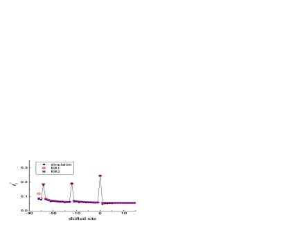
Figure 2: Density profile obtained through a BR relation. $q=0.2,k=26$ and $\ell=12$. The parameters used for fitting are $J$ and $\rho_{R}$.

To summarize, we present the results of the two BR’s in Table 1. If we impose the constraint (26) seriously, we see that the overall fits are tolerable. On the other hand, if we relax this constraint, then there is substantial improvement on all quantities except “$\alpha$”. Clearly, this method, however unsystematic, manages to capture much of the details of the edge effect. Unfortunately, the BR relation fails to produce the long tails in the reader profiles (e.g., Fig. 5 of DSZ_PRE ). Indeed, Eqn.(18) becomes very unstable after about 40 steps, setting a limit on the maximum $k$ to which it can be applied. We believe there are inherent difficulties with this approach (beyond that of machine accuracy), but that is outside the scope of this paper.

Table 1: Summary of fit parameters and $\alpha$ for the two recursion relation schemes. See text for the details. The percentage deviation from the simulation is included in the parenthesis. The last row shows the value of $R^{2}$ from the fit to the profiles in Fig. 2.

	simulation	RR1 (%)	RR2 (%)
$\rho_{R}^{\text{r}}$	0.0550	0.0506 (8.00)	0.0560 (-1.82)
$J$	0.0472	0.0448 (5.08)	0.0478 (-1.23)
$\alpha$	1.0	0.95175 (4.82)	1.5045 (50.45)
$R^{2}$		0.97	0.99

III.2 Finite-segment mean-field (FSMF) theory

Given that we are interested in the edge effect, we can improve on the above method by accounting for the physics of the small $L$ sublattice exactly. This approach follows the work of Chou and Lakatos TomChou , in which the “finite-segment mean-field theory” was developed to understand quantitatively the effects of clustered defects. Here, we generalize this method to particles of size $\ell>1$ and solve the full master equation explicitly for the $L$ sublattice (for small $k$). The key idea is to find the exact expression for the current for this small finite segment and then match it to the result of an infinite system (i.e., the $R$ sublattice). The approximations appear only in the matching conditions and finite size, $O\left(1/N\right)$, effects associated with the latter. We further consider the interplay between the defect rate $q$ and the on-rate $\alpha$. Although our results are based on this simplified model, understanding such interactions elucidates the effects of having a slow codon or a cluster of slow codons near the initiation codon of an mRNA, which is frequently observed in living organisms Chou11 ; Chou14 .

For the $L$ sublattice, the maximum dimension of the transition matrix is $2^{(k+\ell)}$, which requires enormous amounts of computing time even for $k=10$ and $\ell\leq 12$. Fortunately, for $k<\ell$, there can only be $\frac{1}{2}(k^{2}+3k+2\ell+2)$ allowed states in the $k+\ell$ segment. In particular, for $k=1$, the dimension of the transition matrix is $\ell+3$ which is sufficiently small for us to understand the “edge effect.” We illustrate this method through a detailed account for the simplest case ($k=1$), showing the results for both $\ell=1$ and $\ell>1$ (as there are subtle differences for the latter).

Figure 3: Sketch of one slow site $q$ at $k=1$. FSMF matches a two-site TASEP with the rest of the system.

For the case of $k=\ell=1$, we consider two sites, i.e., the entire $L$ sublattice and one site for the $R$ sublattice. Thus, we have only two rates: the entrance rate $\alpha$ and the rate for the slow site $q$. There are four possible configurations ($n_{1}=0,1;n_{2}=0,1$), labeled by $x_{0,1,2,3}$. For convenience, we list these in their binary sequence, namely $x_{0}$ corresponds to state ($0,0$), $x_{1}$ to ($0,1$), etc. The master equation for the evolution of $P_{i}$, the probability to find the system in $x_{i}$ at time $t$ is

$$\partial_{t}P_{i}(t)=\sum_{j}[w_{i}^{j}P_{j}(t)-w_{j}^{i}P_{i}(t)]$$ (29)

where $w_{j}^{i}$ is the rate of $x_{i}$ to $x_{j}$. Referring to Fig. 3 and writing the right hand side of the above as a matrix $\mathbb{W}$ operating on a vector $\vec{P}(t)$, we write explicitly

$$\mathbb{W}=\left(\begin{array}[]{cccc}-\alpha&\beta_{L}&0&0\\ 0&-\alpha-\beta_{L}&q&0\\ \alpha&0&-q&\beta_{L}\\ 0&\alpha&0&-\beta_{L}\end{array}\right)\,\,.$$

Here, $\beta_{L}$ is an effective exit rate, which is to be fixed by matching. The stationary state distribution $\vec{P}^{*}$ is easily found:

$$\vec{P}^{*}=Z^{-1}\left(\begin{array}[]{c}\beta_{L}/\alpha\\ 1\\ (\alpha+\beta_{L})/q\\ \alpha/\beta_{L}\end{array}\right)$$

where $Z=1+\beta_{L}/\alpha+\alpha/\beta_{L}+(\alpha+\beta_{L})/q$ is the normalization factor. The steady state current $J_{L}$ follows readily:

$$J_{L} = \alpha\left\langle 1-n_{1}\right\rangle=q\left\langle n_{1}\left(1-n_{2}\right)\right\rangle=\beta_{L}\left\langle n_{2}\right\rangle$$ (30)

$$= (\alpha+\beta_{L})/Z$$ (31)

Meanwhile, on the $R$ sublattice, we have

$$J_{R}=\left\langle n_{2}\left(1-n_{3}\right)\right\rangle=\left\langle n_{3}\left(1-n_{4}\right)\right\rangle=...$$

which becomes $J_{R}=\rho_{R}(1-\rho_{R})$ for an infinite system in the low density phase. Matching this to the last equation in (30), we arrive at

$$\beta_{L}=1-\rho_{R}$$

and so,

$$J_{L}=J_{R}=\beta_{L}\left(1-\beta_{L}\right)\,\,.$$

Setting this equal to expression (31), we find an equation for $\beta_{L}$. The final answer for the current in this approximation scheme is

$$J_{\text{FSMF}}\left(\alpha,q;\ell=1\right)=\frac{\alpha}{2(q+\alpha)}\{(1+\alpha)(q-\alpha)+\mathcal{R}\}$$ (32)

where $\mathcal{R\equiv}\sqrt{(1+\alpha)(q+\alpha)(\alpha^{2}+\alpha+q-3\alpha q)}$.

We caution that this formula should be used with some care. Though not very transparent, this function monotonically increases with both $q$ and $\alpha$ when both are small. However, beyond a line in the $\alpha$-$q$ unit square, it decreases back to zero. The maximum $J$ on this line is precisely $0.25$, at which point the system enters the MC phase. Substituting $0.25$ into the left of Eqn. (32), we find the phase boundary:

$$q_{c}\left(\alpha\right)=\frac{\alpha(2\alpha+1)}{4\alpha^{2}+2\alpha-1}$$ (33)

beyond which ($q\geq q_{c}$) the MC state prevails.

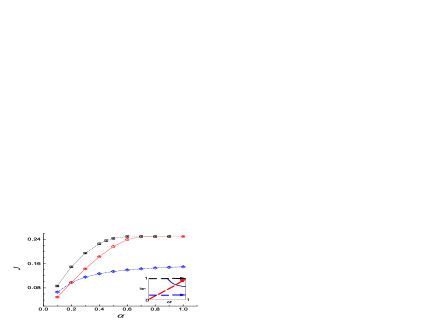
Figure 4: Comparison between the simulations(solid symbols) and the FSMF approximations from Eq. 32 (connected open symbols). Top (black online; $\blacktriangle$, $\Box$): $\alpha=1$; Middle (red online; $\bullet$, $\bigcirc$): $\alpha=q$; and Bottom (blue online; $\blacktriangledown$, $\diamond$): $q=0.2$. In all cases, $\ell=1$ and $N=1000$. The inset follows the same color coding scheme. See text for details.

To further appreciate the quality of this theory, we present the comparison between its predictions and simulation data in Fig. 4. Specifically, we show three typical scans through the $\alpha$-$q$ plane, sketched in the inset of Fig. 4. The upper-right corner represents the MC phase (where $J=0.25$), with the solid (black online) curve being $q_{c}\left(\alpha\right)$ in Eqn. (33). The color-coding in the inset matches the data in the main plot of Fig. 4. Here, the statistical error associated with the simulations is estimated to be around $0.01\%$. We observe excellent agreement (within $1\%$) between the data and the theory results. Needless to say, we can extend this approach, with some labor, to $k>1$. Since we doubt that the agreement would be significantly different, we believe there is no need to pursue this investigation further. Instead, we turn next to the more interesting systems with extended objects.

Generalizing to the case with $\ell>1$, we need to account for two novel aspects. One important difference is the current matching condition: Instead of $J_{L}=\beta_{L}\simeq(1-\rho_{R})$, we use the MGP result for $\ell>1$ case and

$$\beta_{L}\simeq\frac{1-\rho_{R}}{\rho_{i+\ell}^{\text{r}}+1-\rho_{R}}\simeq\frac{\ell(1-\rho_{R})}{\ell-\bar{\ell}\rho_{R}}\,\,.$$ (34)

The other new item is that, since we expect some “period-$\ell$” structure, we could consider all $k$ up to $\ell$ and still restrict ourselves to having only one particle in the $L$ sublattice. Following the spirit of our analysis above, we also wish to account for the effects (on the $L$ sublattice) due to a particle which just moved into the $R$ sublattice. With at most two particles in our finite segment, the exclusion “at a distance” means that we need to study a system with $k+\ell$ sites. Fortunately, the configuration space (for, say, the reader occupations $\left\{r_{i}\right\}$) is still manageably small. Thus, there is just one 0-particle state, $(k+\ell)$ 1-particle states, and $k\left(k+1\right)/2$ 2-particle states. We demonstrate the case for $k=1$ here. Let us label the 0-particle state by $x_{0}$, the state with a reader in site $i$ by $x_{\ell+2-i}$ ($i=1,...,\ell+1$), and finally, the 2-particle state by $x_{\ell+2}$. To be pedantic, we show the explicit set of occupation numbers $\left\{r_{j}\right\}$ corresponding to these $x$’s:

$$x_{0} \Leftrightarrow \left(\begin{array}[]{cccccc}0&0&\cdots&\cdots&0&0\end{array}\right)$$ (36)

$$x_{1} \Leftrightarrow \left(\begin{array}[]{cccccc}0&0&\cdots&\cdots&0&1\end{array}\right)$$ (38)

$$x_{2} \Leftrightarrow \left(\begin{array}[]{cccccc}0&0&\cdots&\cdots&1&0\end{array}\right)$$ (41)

$$\vdots$$

$$x_{\ell} \Leftrightarrow \left(\begin{array}[]{cccccc}0&1&\cdots&\cdots&0&0\end{array}\right)$$ (43)

$$x_{\ell+1} \Leftrightarrow \left(\begin{array}[]{cccccc}1&0&\cdots&\cdots&0&0\end{array}\right)$$ (45)

$$x_{\ell+2} \Leftrightarrow \left(\begin{array}[]{cccccc}1&0&\cdots&\cdots&0&1\end{array}\right)$$ (47)

The advantage of this slightly peculiar labeling is that it reduces to the $\ell=1$ case easily.

To find the current $J(\alpha,q,\ell)$ for $\ell>1$, we need to compute the new transition matrix $\mathbb{W}$. With the configurations clear in our minds, we simply write:

$$\mathbb{W}=\left(\begin{array}[]{cccccccc}-\alpha&\beta_{L}&0&\cdots&\cdots&\cdots&0&0\\ 0&-\alpha-\beta_{L}&\beta_{L}&0&\cdots&\cdots&\vdots&\vdots\\ 0&0&-\beta_{L}&\beta_{L}&0&\cdots&\vdots&\vdots\\ \vdots&\vdots&0&-\beta_{L}&\beta_{L}&0&\vdots&\vdots\\ \vdots&\vdots&\vdots&\vdots&\vdots&\vdots&\vdots&\vdots\\ 0&&&&&-\beta_{L}&q&0\\ \alpha&0&\vdots&\vdots&&&-q&\beta_{L}\\ 0&\alpha&0&0&&&0&-\beta_{L}\end{array}\right)\,\,$$ (48)

Similar to the $\ell=1$ case, we find

$$\vec{P}^{*}=Z^{-1}\left(\begin{array}[]{c}(\beta_{L}/\alpha)\\ 1\\ (\alpha+\beta_{L})/\beta_{L}\\ \vdots\\ (\alpha+\beta_{L})/\beta_{L}\\ (\alpha+\beta_{L})/q\\ \alpha/\beta_{L}\end{array}\right)$$

to be the same, except for $\bar{\ell}$ more entries of $(\alpha+\beta_{L})/\beta_{L}$ in the middle. Thus,

$$Z=1+\beta_{L}/\alpha+\alpha/\beta_{L}+(\alpha+\beta_{L})/q+\bar{\ell}(\alpha+\beta_{L})/\beta_{L}$$

Meanwhile, we still have $J_{L}=(\alpha+\beta_{L})/Z$. Finally, matching $J_{L}$ with $J_{R}=\rho_{R}(1-\rho_{R})/\left(\ell-\bar{\ell}\rho_{R}\right)$ and using Eqn. (34), we arrive at the solution for general $\ell$ (and $k=1$ ):

$$J_{\text{FSMF}}(\alpha,q,\ell)=\frac{\alpha}{2(q+\alpha)}\frac{q-\alpha+\mathcal{R}(1+\alpha)^{-1}+\bar{\ell}\left[q(1-\alpha)+\mathcal{R}q\left(q+\alpha\right)^{-1}\right]}{(1+\alpha)^{-1}+\bar{\ell}\left[1+\bar{\ell}\alpha q(q+\alpha)^{-1}\right]}$$ (49)

We have written $J_{\text{FSMF}}$ in a form that clearly reduces to Eqn. (32) for $\ell=1$. Given the shifted phase boundaries for $\ell>1$, the system enters the MC phase when:

$$q_{c}=\frac{\alpha\hat{\chi}(\alpha+1-\hat{\chi})}{\alpha(\alpha+1-\hat{\chi})-\hat{\chi}(1-\hat{\chi})}$$ (50)

In the next section, we will summarize our findings along with some comparisons to Monte Carlo simulation data.

IV Summary and outlook

We investigated how a single defect site near the lattice boundary (small $k$) influences the steady state properties of the system for both point particles and those of length $\ell>1$. The simplest “mean-field” approaches – NMF and SKL – are unsuitable, since both rely on matching two infinite TASEP’s across a defect and cannot address the issue of $k$-dependence. Instead, we considered two more sophisticated levels of mean-field methods, with complementary strengths and weaknesses. One method, first used by MacDonald, et. al. MG (MGP), is based on a recursion relation for the density profile. The advantage of MGP is that, up to moderate $k$ values, its predictions for both the profile and the current are reasonably good. The weakness is that we can access these predictions only numerically so that the dependence on the control parameters $\alpha,q,k,$ and $\ell$ remains obscure. It is also unclear how to systematically improve on this approach. The other method, based on an exact account of the physics of the first $k+\ell$ sites, is a generalization of the finite segment mean-field (FSMF) theory of Chou and Lakatos TomChou . The strengths of this method are many. Based on the steady state solution to the full master equation, it can be improved systematically. Its predictions agree with simulations exceedingly well and provide analytic expressions so that the dependence on $\left(\alpha,q,\ell\right)$ can be appreciated. Both methods are obviously severely restricted to a relatively small range of $k$’s. In MGP, the limitation arises from the extreme sensitivity of the recursion relation and, in FSMF, an exponential increase (in the worst scenario) in the size of the transition matrix. Moreover, some of the long tails in the “edge effect” extend up to $k\sim 50$ DSZ ; DSZ_PRE , well beyond the present reach of either approach. Hopefully, more efficient approaches will be developed in the future.

To summarize, we find three successively better methods to describe a TASEP with a defect near the entrance, for $\ell\geq 1$. To illustrate, we present the results of all three mean-field approaches, along with simulation data, in Tables 2 and 3. Both concern the case with $\alpha=\beta=1$ and $k=1$; the difference being $\ell=1,2$ in the two Tables. We see that, by accounting for exclusion at a distance, MGP (with the fit through $RR1$) clearly succeeds better than NMF when $\ell>1$. Meanwhile, it is hardly surprising that an exact treatment of the finite segment before the defect is superior to both.

Though not displayed explicitly, similar improvements are found to hold for $\ell$ up to $12$. Finally, if we use $J_{\text{FSMF}}$ for $k=1$ and $J_{\text{NMF}}$ for $k\gg 1$ (i.e., deep in the bulk), we arrive at a prediction for $\Delta_{1}\left(q\right)\equiv\left.J_{q}(k=1)\right/J_{q}(k\rightarrow\infty)$, defined in DSZ_PRE . The remarkable non-monotonic behavior in $\Delta_{1}$ (shown in Fig. 7 of DSZ_PRE ) is well captured by the combination of these two mean-field approaches.

Table 2: Different mean-field approximations for the current $J(q)$ for the case $\alpha=\beta=1$, $k=1$ and $\ell=1$. Simulation results are based on a lattice with $L=1000$.

$q$ $J_{\text{NMF}}$ $J_{\text{MGP}}$ $J_{\text{FSMF}}$ simulation 0.1 0.0826 0.0833 0.0863 0.0864 0.2 0.1389 0.1421 0.1498 0.1490 0.3 0.1775 0.1848 0.1954 0.1941 0.4 0.2041 0.2153 0.2261 0.2248 0.5 0.2222 0.2361 0.2440 0.2432 0.6 0.2344 0.2476 0.2500 0.2502

Table 3: Different mean-field approximations for the current $J(q)$ for the case $\alpha=\beta=1$, $k=1$, and $\ell=2$. Simulation results are based on a lattice with $L=1000$.

$q$	$J_{\text{NMF}}$	$J_{\text{MGP}}$	$J_{\text{FSMF}}$	simulation
0.1	0.0758	0.0763	0.0788	0.0771
0.2	0.1190	0.1213	0.1266	0.1231
0.3	0.1442	0.1484	0.1543	0.1509
0.4	0.1587	0.1639	0.1680	0.1665
0.5	0.1667	0.1708	0.1715	0.1717

Beyond our investigations here, there is ample room for future research. In an open TASEP, there are two “edges” and so, two possible “edge effects.” We reported findings for only one. When the slow site is near the exit ($k\simeq L$), the current is also observed to increase ETD . However, due to lack of particle-hole symmetry for $\ell>1$, this increase is not the same as the case for small $k$. Further, there are serious complications associated with the profile, especially for small $q$ (e.g., Fig. 5 in DSZ_PRE ). Thus, it would be desirable to find better methods to understand these peculiarities quantitatively. Similarly, we should explore the “edge effect” for $q>1$. When a “fast site” is deep in the bulk, it has little effect on the current. However, its effects if located near the edges, especially near the exit end, are yet to be discovered. Beyond one defect, there are obvious questions concerning two or more defects. It was found that two equally slow sites deep in the bulk “interact” DSZ_PRE , in the sense that the overall current is significantly suppressed when they are located near each other. Much less has been investigated when the two defects are associated with different rates. Both mean-field methods can easily be extended to study such issues, especially when the two sites are near each other. At the other extreme, we face a completely inhomogeneous TASEP. But this is precisely the scenario more relevant for protein synthesis in vivo. In this sense, there is much to be done before we reach the goal of a realistic model for understanding the biological process of translation.

References

References

- (1) Spitzer F 1970 Adv. Math. 5 246
- (2) Derrida B, Domany E, and Mukamel D 1992 J. Stat. Phys. 69 667
- (3) Derrida B, Evans M R, Hakim V, and Pasquier V 1993 J. Phys. A: Math. Gen. 26 1493
- (4) Schütz G M and Domany E 1993 J. Stat. Phys. 72 277
- (5) Derrida B 1998 Phys. Rep. 301 65
- (6) Schütz G M 2000 Phase Transition and Critical Phenomena edited by Domb C and Lebowitz J L (Academic Press, San Diego)
- (7) Kardar M, Parisi G, and Zhang Y C 1986 Phys. Rev. Lett. 56 889
- (8) Wolf D E and Tang L H 1990 Phys. Rev. Lett. 65 1591
- (9) MacDonald C, Gibbs J, and Pipkin A 1968 Biopolymers 6 1; MacDonald C and Gibbs J 1969 Biopolymers 7 707
- (10) Shaw L B, Zia R K P, and Lee K H 2003 Phys. Rev. E 68 021910
- (11) Chou T and Lakatos G 2004 Phys. Rev. Lett. 93 198101
- (12) Shaw L B, Sethna J P and Lee K H 2004 Phys. Rev. E 70 021901
- (13) Shaw L B, Kolomeisky A B and Lee K H 2004 J. Phys. A: Math. Gen. 37 2105
- (14) Chowdhury D, Santen L and Schadschneider A 1999 Curr. Sci. 77 411
- (15) Popkov V, Santen L, Schadschneider A and Schütz G M 2001 J. Phys. A: Math. Gen. 34 L45
- (16) Dong J J, Schmittmann B and Zia R K P 2007 J. Stat. Phys. 128 21
- (17) Heinrich R and Rapoport T 1980 J. Theor. Biol. 86 279
- (18) Kang C and Cantor C 1985 J. Mol. Struct. 181 241
- (19) Lakatos G and Chou T 2003 J. Phys. A: Math. Gen. 36 2027
- (20) Dong J J, Schmittmann B and Zia R K P 2007 Phys. Rev. E 76 051113
- (21) Harris R J and Stinchcombe R B 2004 Phys. Rev. E 70 016108
- (22) Foulaadvand M E, Chaaboki S and Saalehi1 M 2007 Phys. Rev. E 75 011127
- (23) Edwards S F and Anderson P W 1975 J. Phys. F 5 965; Mézard M, Parisi G and Virasoro M A 1987 Spin glass theory and beyond (World Scientific, Singapore)
- (24) Kolomeisky A 1998 J. Phys. A: Math. Gen. 31 1153
- (25) Greulicha P and Schadschneider A 2008 Physica A 387 1972
- (26) Chou T 2007 private communication
- (27) Phoenix D A and Korotkov E 1997 FEMS Microbiol. Lett. 155 63
- (28) Zhang S, Goldman E, and Zubay G 1994 J. Theor. Biol. 170 339
- (29) Details may be found in Dong J J 2008 Inhomogeneous Totally Asymmetric Simple Exclusion Processes: Simulations, Theory and Application to Protein Synthesis, PhD thesis, Virginia Tech