Nonequilibrium Cotunneling through a Three-Level Quantum Dot

Abstract

We calculate the nonlinear cotunneling conductance through a quantum dot with 3 electrons occupying the three highest lying energy levels. Starting from a 3-orbital Anderson model, we apply a generalized Schrieffer-Wolff transformation to derive an effective Kondo model for the system. Within this model we calculate the nonequilibrium occupation numbers and the corresponding cotunneling current to leading order in the exchange couplings. We identify the inelastic cotunneling thresholds and their splittings with applied magnetic field, and make a qualitative comparison to recent experimental data on carbon nanotube and InAs quantum-wire quantum dots. Further predictions of the model such as cascade resonances and a magnetic-field dependence of the orbital level splitting are not yet observed but within reach of recent experimental work on carbon nanotube and InAs nanowire quantum dots.

The Kondo effect has been observed in a number of different quantum dot (QD), and single molecule devices Goldhaber:98 ; Cronenwett:98 ; Wiel:00 ; Nygaard:00 ; Sand:06 . The effect is manifested as a sharp conductance peak at zero bias-voltage, developing when the temperature is lowered beyond the characteristic Kondo temperature. It relies on a spin-degenerate ground-state on the quantum dot, which gives rise to logarithmically singular spin-flip scattering of the conduction electrons traversing the dot. Meanwhile, for quantum dots with sufficiently small level spacings or slightly broken degeneracies, the Kondo-peak at zero bias voltage can be flanked by two or more satellite steps or even peaks in the nonlinear conductance. Such inelastic cotunneling features are often seen in both GaAsZumbuhl:04 , Carbon nanotube Babic:04 ; Paaske:06 ; Holm:08 (CNT) and InAs-wire Sand:06 ; Csonka:08 quantum dots, but in most cases they are masked by charge-excitations which can be nearby in energy and for this reason they have not received much attention.

Single-molecule transistors, on the other hand, exhibit a much larger charging energy, $E_{C}$ ($\sim$ 100 meV instead of 5 meV, say, for a typical quantum dot). At the same time, these molecular systems often display a number of degeneracies which are weakly broken once the molecule is contacted by source, and drain electrodes, thus inducing splittings of the order of a few meV. Most recently, this was seen in Refs. Osorio:07, ; Roch:08, , where junctions holding an OPV5, or a $C_{60}$ molecule, respectively, showed a very clear singlet-triplet splitting on the scale of 1 meV together with a charging energy of the order of 100 meV. This is a very convenient separation of energy scales which raises the experimental resolution of inelastic cotunneling phenomena to new standards. Nevertheless, given the simpler level-structure of most conventional QD-devices, it is desirable to revisit and understand the details of interorbital transitions better in these systems. This is what we set out to do in the present paper.

In the following, we study the case of a quantum dot occupied by an odd number of electrons, featuring a spin-doublet groundstate, giving rise to a zero-bias Kondo peak, but with additional orbitals/levels leading to flanking inelastic cotunneling steps or peaks. The basic 3-orbital Anderson model is illustrated in Fig. 1 and will be shown to host a variety of different I-V-characteristics depending on the relative magnitudes of the 6 different tunneling-amplitudes.

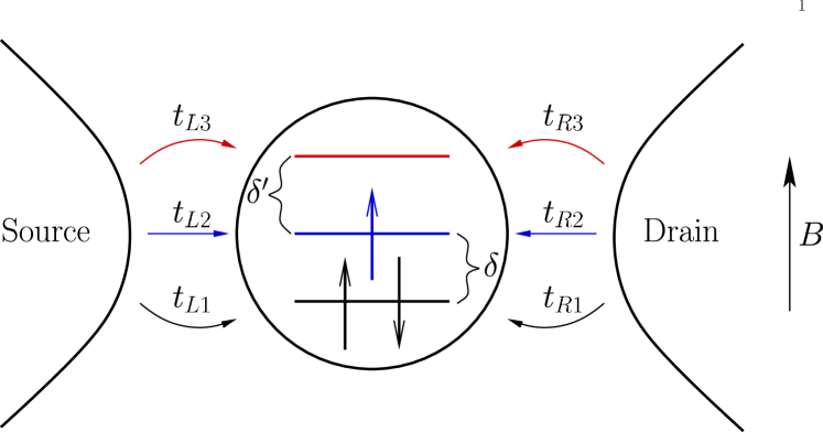
Figure 1: Illustration of the setup. We consider the three highest-lying levels of a quantum dot, separated by energies $\delta$, and $\delta^{\prime}$. Both orbitals are connected to source (left lead) and drain (right lead) via 6 different tunnel couplings $t_{\alpha n}$. The dot is in the Coulomb blockade regime with the three levels adjusted by a gate to accommodate exactly 3 electrons.

This 3-orbital model was briefly discussed by some of the present authors in Ref. Sand:06, (cf. inset in Fig. 4b), where it was invoked to explain the relatively sharp peaks at finite bias flanking a zero-bias Kondo-effect observed in an InAs quantum-wire dot Sand:06 . The measured nonlinear conductance curves for varying applied magnetic fields are shown in Fig. 2. This experiment constitutes one of the rare cases where such side-peaks could actually be resolved.

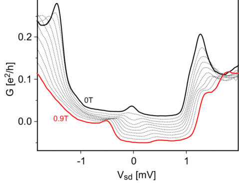
Figure 2: (color online) Differential conductance, $G$, as a function of bias voltage, $V_{sd}$, for an InAs-wire based quantum dot at $T=0.3$ K. The data were taken at magnetic fields (perpendicular to the wire) $B=0$ (thick), 0.1 (dotted), …, 0.9 T (red) and the curves were offset by 0.008 $e^{2}/h$ for clarity. The data were taken for an odd occupied Coulomb diamond at gate voltage $V_{g}=-2.35$ V Sand:06 .

As one further example, Fig. 3 shows similar data recorded on a single-walled carbon nanotube (CNT) quantum dot (QD). Both sets of measurements show well-defined peaks which split into weak thresholds on applying a magnetic field. Notice the different field-strengths needed in the two experiments, reflecting the roughly 4 times larger spin-orbit enhanced g-factor in InAs as compared to the CNT.

The bulk of this paper deals with leading order nonequilibrium cotunneling for the 3-orbital Anderson model in the Kondo-regime. First we derive an effective cotunneling, or Kondo model for a system with three electrons distributed on the three orbitals. From this effective low-energy model we then proceed to calculate the I-V characteristics to leading (second) order in the cotunneling amplitude. In section III we discuss some of the salient transport features of this system and in section IV we discuss the CNT and the InAs data shown in Figs. 2 and 3.

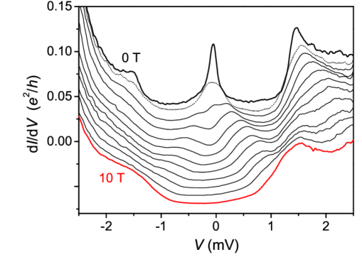
Figure 3: (color online) Differential conductance, $dI/dV$, as a function of bias voltage, $V$, for a carbon nanotube quantum dot at $T=0.08$ K. The data were taken at magnetic fields (perpendicular to the tube) $B=0$ (thick), 0.1 (dotted), 1 (thin), 2, 3, …, 9, 10 T (red) and the curves were offset by 0.008 $e^{2}/h$ for clarity. The data were taken for an odd occupied Coulomb diamond at gate voltage $V_{g}=-4.96$ V Paaske:06 . (Note that at finite magnetic fields features are broadened due to noise induced by the magnet power supply).

In this context we point out additional properties of such samples which can be read off the dI-dV characteristic.

I Effective low-energy Kondo model

The 3-orbital Anderson model corresponding to the setup in Fig. 1 we write as

$$H=H_{\mathrm{lead}}+H_{\mathrm{dot}}+H_{\mathrm{tun}}\,.$$ (1)

The leads are described by the non-interacting Hamiltonian

$$H_{\mathrm{lead}}=\sum_{\begin{subarray}{c}\alpha=L,R\\ \mathbf{k}\sigma\end{subarray}}(\varepsilon_{\mathbf{k}}-\mu_{\alpha})c_{\alpha\mathbf{k}\sigma}^{\dagger}c_{\alpha\mathbf{k}\sigma}^{\phantom{\dagger}}$$ (2)

where $\alpha=L,R$ labels the leads, assumed to be in equilibrium at chemical potentials $\mu_{\alpha}$. The operator $c_{\alpha\mathbf{k}\sigma}^{\dagger}$ creates an electron in lead $\alpha$ of momentum $\mathbf{k}$ and spin $\sigma$. A simple constant interaction model is used to describe the quantum dot itself in terms of three non-degenerate orbitals with one common Coulomb repulsion $U(\sim E_{C})$:

$$H_{\mathrm{dot}}= \sum_{n\sigma}\varepsilon_{n\sigma}f_{n\sigma}^{\dagger}f_{n\sigma}^{\phantom{\dagger}}$$

$$+ \frac{1}{2}U\sum_{n\sigma}\sum_{m\sigma^{\prime}}f_{n\sigma}^{\dagger}f^{\phantom{\dagger}}_{n\sigma}\Big{(}f_{m\sigma^{\prime}}^{\dagger}f^{\phantom{\dagger}}_{m\sigma^{\prime}}-1\Big{)},$$ (3)

where $n,m=1,2,3$ label the orbitals on the dot and $f_{n\sigma}^{\dagger}$ creates an electron in orbital $n$ with spin $\sigma$ and with energy $\epsilon_{n\sigma}=\epsilon_{n}-\frac{1}{2}\sigma g\mu_{B}B$ where $\epsilon_{2}\equiv\epsilon_{1}+\delta$, and $\epsilon_{3}=\epsilon_{2}+\delta^{\prime}$, with level-splittings denoted by $\delta$ and $\delta^{\prime}$. Finally, the tunneling Hamiltonian,

$$H_{\mathrm{tun}}=\sum_{\begin{subarray}{c}\alpha=L,R\\ n\sigma\end{subarray}}\left(t_{\alpha n}c_{\alpha\sigma}^{\dagger}f^{\phantom{\dagger}}_{n\sigma}+h.c.\right),$$

describes the coupling of the leads to the dot via six independent tunneling amplitudes $t_{\alpha n}$, see illustration in Fig. 1. For later convenience, we have introduced the local conduction electron operators $c_{\alpha\sigma}^{\dagger}=\sum_{\mathbf{k}}c_{\alpha\mathbf{k}\sigma}^{\dagger}$.

We now restrict our attention to the Kondo-regime in which all three orbitals are sufficiently narrow compared to the charging energy to effectively suppress all charge-fluctuations, leaving the dot with a well defined occupation of 3 electrons in three orbitals. Since the experimental data in Figs. 2 and 3 do not resolve higher lying peaks corresponding to excited states with two electrons in orbital 3, we shall simplify our model further by also omitting these higher lying 3-particle states. In the experiments, the cotunneling thresholds for these higher lying states must be comparable to the charging-energy and are therefore masked by charge-fluctuations. As mentioned earlier, this is a typical problem of the relatively large quantum dots (compared to single-molecule junctions) which provide a rather poor separation of energy-scales. Altogether, we are now left with an effective low-energy Hilbert-space spanned by the six lowest lying three-electron states:

$$|s\sigma\rangle =f_{2\sigma}^{\dagger}f_{1\downarrow}^{\dagger}f_{1\uparrow}^{\dagger}|\mathrm{vac}\rangle,$$

$$|h\sigma\rangle =f_{2\downarrow}^{\dagger}f_{2\uparrow}^{\dagger}f_{1\sigma}^{\dagger}|\mathrm{vac}\rangle,$$ (4)

$$|p\sigma\rangle =f_{3\sigma}^{\dagger}f_{1\downarrow}^{\dagger}f_{1\uparrow}^{\dagger}|\mathrm{vac}\rangle.$$

We label these three-body states by indices $a,b=\{s,h,p\}$ (i.e. {spin, hole, particle}), together with the spin-index $\sigma=\{\uparrow,\downarrow\}$. The notation is obvious from the illustration of the states in Fig. 4.

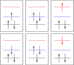
Figure 4: Illustration of the three lowest lying energy states that are taken into account in the effective cotunneling model of the 3-orbital Anderson model. From left to right: spin, hole and particle states.

The energies of these states are

$$E_{s\sigma} =2\varepsilon_{1}+\varepsilon_{2}+3U-\frac{1}{2}\sigma g\mu_{B}B,$$

$$E_{h\sigma} =\varepsilon_{1}+2\varepsilon_{2}+3U-\frac{1}{2}\sigma g\mu_{B}B,$$ (5)

$$E_{p\sigma} =2\varepsilon_{1}+\varepsilon_{3}+3U-\frac{1}{2}\sigma g\mu_{B}B.$$

In the case of equidistant energy levels $E_{h\sigma}=E_{p\sigma}$ and the two excited states, corresponding to respectively an electron moved to orbital 3 or a hole moved to orbital 1, are degenerate. The energy $\varepsilon_{2}$ is set by tuning the voltage on a gate and here we choose it such that the 3-particle state will be lower in energy than both the 2, and the 4-particle states, that is:

$$E_{2e^{-}}=2\varepsilon_{1}+U >E_{3e^{-}},$$ (6)

$$E_{4e^{-}}=2\varepsilon_{1}+2\varepsilon_{2}+6U >E_{3e^{-}}.$$

In the following, we shall choose $\varepsilon_{2}=-5/2\ U$, which places the system at the particle-hole symmetric point where $E_{4e^{-}}-E_{3e^{-}}=E_{2e^{-}}-E_{3e^{-}}=U/2$, with $E_{3e^{-}}=E_{s\sigma}$ as the ground state.

In order to eliminate charge-fluctuations from the 3-orbital Anderson model (1), we employ a generalized Schrieffer-Wolff transformation Schrieffer:66 which serves to eliminate the tunneling-term, $H_{\mathrm{tun}}$, and retains only terms of second order in the tunneling-amplitudes in the form of an effective cotunneling, or Kondo Hamiltonian:

$$H_{\mathrm{eff}}=H_{\mathrm{lead}}+\sum_{a\sigma}E_{a\sigma}|a\sigma\rangle\langle a\sigma|+H_{\mathrm{int}}.$$ (7)

The effective interaction now takes the form of a spin/orbital exchange-term:

$$H_{\mathrm{int}}=\sum_{\begin{subarray}{c}\alpha\beta,ab\\ \sigma^{\prime}\sigma\end{subarray}}\!\!J_{\alpha\beta}^{ab}\left[\frac{1}{2}\mathbf{S}_{ab}\cdot\boldsymbol{\tau}_{\sigma^{\prime}\sigma}-\hat{P}_{ab}\delta_{\sigma^{\prime}\sigma}\right]c_{\alpha\sigma^{\prime}}^{\dagger}c^{\phantom{\dagger}}_{\beta\sigma},$$ (8)

in terms of the vector of Pauli matrices, $\boldsymbol{\tau}$, the spin-operator for the quantum-dot

$$\mathbf{S}_{ab}=\frac{1}{2}\sum_{\sigma\sigma^{\prime}}|a\sigma\rangle\boldsymbol{\tau}_{\sigma\sigma^{\prime}}\langle b\sigma^{\prime}|,$$ (9)

and the potential scattering term $\hat{P}_{ab}=\hat{P}_{ab}^{\mathrm{inel}}+\hat{P}_{ab}^{\mathrm{el}}$ which consists of an inelastic scattering which involves a change in the orbital state

$$\hat{P}^{\mathrm{inel}}_{ab}= \frac{1}{4}\big{(}\delta_{a,s}\delta_{b,p}+\delta_{a,p}\delta_{b,s}-\delta_{a,s}\delta_{b,h}-\delta_{a,h}\delta_{b,s}\big{)}$$

$$\hskip 22.76219pt\times\sum_{\sigma^{\prime}}|a\sigma^{\prime}\rangle\langle b\,\sigma^{\prime}|.$$ (10)

and the elastic scattering which occurs via empty levels, i.e. level $3$ for $|s\rangle$ and $|h\rangle$ and level $2$ for $|p\rangle$,

$$\hat{P}^{\mathrm{el}}_{ab}= \frac{1}{4}\delta_{a,b}\sum_{\tilde{a}}\big{(}\delta_{\tilde{a},s}\delta_{a,p}+\delta_{\tilde{a},h}\delta_{a,p}+\delta_{\tilde{a},p}\delta_{a,s}\big{)}$$

$$\hskip 22.76219pt\times\sum_{\sigma^{\prime}}|\tilde{a}\sigma^{\prime}\rangle\langle\tilde{a}\sigma^{\prime}|.$$ (11)

To lowest order a transition between the excited states $|p\rangle$ and $|h\rangle$ is not possible.

A constant energy offset arising in the Schrieffer-Wolff transformation is neglected and so are further potential scattering terms. These lead only to a constant offset in the differential conductance of the order of $\delta/U^{2}$, which can be neglected in our qualitative study. Details of the calculation, including the expression for the coupling functions $J_{\alpha\beta}^{ab}$, are given in appendix A.

Note that when calculating the effective cotunneling amplitudes in the appendix, we retain the differences in energy-denominators of the different amplitudes, i.e. at this stage we do not make the approximation that $U\gg\delta^{(\prime)}$. The according differences in amplitudes expresses the broken orbital symmetry of the model, even with all six tunneling-amplitudes being equal. Nevertheless, in order for the Schrieffer-Wolff transformation to be meaningful, we must demand these differences to be small, and in all our numerical calculations we therefore choose a large charging energy ($U\sim 100\delta$) which effectively makes all energy denominators equal. In other words, retaining $\delta^{(\prime)}$ in the denominators of the cotunneling amplitudes would require a more careful treatment of charge-fluctuations.

II Nonequilibrium perturbation theory

When the bias voltage is large enough to populate the excited states on the dot, these will no longer be thermally occupied Paaske:04a ; Parcollet:02 . This effect is incorporated in the Keldysh component Dyson equation expressed in terms of nonequilibrium Green functions Rammer:86 ; Haug:96 with self-energies calculated to leading (second) order in the effective cotunneling amplitudes or exchange couplings $\nu_{F}J_{\alpha\beta}^{ab}\ll 1$. Following the approach taken in Ref. Paaske:04a, , we employ a pseudo-fermion representation for the dot-states, with operators defined by $d^{\dagger}_{a\sigma}|0\rangle\equiv|a\sigma\rangle$ and $\langle 0|d^{\phantom{\dagger}}_{a\sigma}\equiv\langle a\sigma|$, and subject to the constraint $\mathcal{Q}=\sum_{a,\sigma}d^{\dagger}_{a\sigma}d^{\phantom{\dagger}}_{a\sigma}=1$. The constraint is enforced with the aid of a Lagrange multiplier $\lambda$, included as an additional term, $H_{\lambda}=\lambda\sum_{a,\sigma}d^{\dagger}_{a\sigma}d^{\phantom{\dagger}}_{a\sigma}$, in the Hamiltonian Abrikosov:65 . The exact projection to the physical Hilbert space is effected by taking the limit $\lambda\to\infty$. We shall need the non-equilibrium Green’s functions:

$$\mathcal{G}_{ab,\sigma\sigma^{\prime}}(\tau,\tau^{\prime}) =-\mathrm{i}\left\langle T_{\mathrm{C_{K}}}\big{(}d^{\phantom{\dagger}}_{a\sigma}(\tau)d_{b\sigma^{\prime}}^{\dagger}(\tau^{\prime})\big{)}\right\rangle$$ (12)

$$G_{\alpha\beta,\sigma\sigma^{\prime}}(\tau,\tau^{\prime}) =-\mathrm{i}\left\langle T_{\mathrm{C_{K}}}\big{(}c^{\phantom{\dagger}}_{\alpha\sigma}(\tau)c_{\beta\sigma^{\prime}}^{\dagger}(\tau^{\prime})\big{)}\right\rangle$$ (13)

with $T_{C_{K}}$ being the time ordering operator along the Keldysh contour. Calligraphic letters denote pseudo-fermion, italic letters conduction electron Green’s functions.

The retarded and advanced Green’s functions can be calculated like in the equilibrium case directly from the Dyson equation. The pseudo-fermion spectral function is obtained from the imaginary part of the retarded Green’s function,

$$\mathcal{A}_{aa,\sigma}=-2\ {\rm Im}\left[\frac{1}{\omega-\omega_{a\sigma}-\Sigma_{aa,\sigma}^{R}}\right],$$ (14)

and takes the approximate form of a Lorentzian at the resonance frequency $\omega_{a\sigma}=\varepsilon_{a\sigma}+\lambda$ and of width $\Gamma_{aa,\sigma}=-2\ {\rm Im}[\Sigma_{aa,\sigma}^{R}]$. Since the spectral function appears in later evaluations only in convolution with functions that vary on a larger energy scale than $\Gamma_{aa,\sigma}$, we approximate it by a simple delta-function:

$$\mathcal{A}_{aa,\sigma}(\omega)=2\pi\delta(\omega-\omega_{a\sigma}).$$ (15)

The lesser function is found from the quantum Boltzmann equation (QBE), or generalized Kadanoff-Baym equation:

$$\Gamma_{aa,\sigma}(\omega)\mathcal{G}^{<}_{aa,\sigma}(\omega)=\mathcal{A}_{aa,\sigma}(\omega)\Sigma^{<}_{aa,\sigma}(\omega).$$ (16)

Within the delta-function (quasiparticle) approximation for the spectral function, this equation can be solved using the following ansatz:

$$\mathcal{G}_{aa,\sigma}^{<}(\omega)=\mathrm{i}n_{a\sigma}\mathcal{A}_{a\sigma}(\omega),$$ (17)

through which the QBE takes the form of a simple rate-equation.

The conduction electrons are assumed to remain in thermal equilibrium and are therefore characterized simply by their respective chemical potentials together with a simple flat-band approximation for the momentum-summed spectral functions, or local conduction electron density of states (DOS) at the contact,

$$A(\omega)=2\pi\nu_{F}\theta(D-|\omega|),$$ (18)

in terms of the DOS at the Fermi surface, $\nu_{F}$, and half bandwidth $D$.

II.1 Nonequilibrium occupation numbers

In writing the QBE in Eq. (16), we have tacitly assumed the pseudo-fermion self-energies to be diagonal in both spin, and orbital indices. Neglecting spin-orbit interactions spin is a conserved quantum number and the self-energy will therefore be diagonal in this index. This does not hold for the orbital quantum number $a$ and off-diagonal terms, $\Sigma_{ab,\sigma}$, can arise. Nevertheless, in the regime studied here for which the level splittings $\delta,\delta^{\prime}$ are assumed to be much larger than level broadenings, $\Gamma_{a}$, energy conservation suppresses such off-diagonal terms and the self energy can safely be assumed to be diagonal. For an example in which off-diagonal contributions remain important we refer the interested reader to Ref. Koerting:08, .

Thus neglecting off-diagonal self-energies and using Eq. (17), the QBE in Eq. (16) takes the following form:

$$n_{a\sigma}=\mathrm{i}\frac{\Sigma_{a\sigma}^{<}(\omega_{a\sigma})}{\Gamma_{a\sigma}(\omega_{a\sigma})}.$$ (19)

The self energy $\Sigma_{a\sigma}^{<}$ itself depends on the occupation numbers and this therefore constitutes a set of six coupled equations for six unknown occupation numbers. These equations are underdetermined and should therefore be solved together with the constraint $\mathcal{Q}=\sum_{a\sigma}n_{a\sigma}=1$. More details of the actual calculation of pseudo-fermion self-energies are given in appendix B.

II.2 Cotunneling current

We obtain the current operator directly from the time-derivative of the density operator at the contact in the left lead, say (see Ref. Paaske:04a, and references therein). With $n_{L}=\sum_{\sigma}c_{L\sigma}^{\dagger}c^{\phantom{\dagger}}_{L\sigma}$, one finds

$$j_{L} =e\frac{dn_{L}}{dt}=\frac{\mathrm{i}e}{\hbar}\left[n_{L},H_{\mathrm{int}}\right]$$

$$=\sum_{\alpha,ab,\sigma^{\prime}\sigma}\bigg{\{}\frac{1}{2}\mathbf{S}_{ab}\cdot\boldsymbol{\tau}_{\sigma\sigma^{\prime}}\left(J_{LR}^{ab}c_{L\sigma^{\prime}}^{\dagger}c^{\phantom{\dagger}}_{R\sigma}-J_{RL}^{ab}c_{R\sigma^{\prime}}^{\dagger}c^{\phantom{\dagger}}_{L\sigma}\right)$$

$$\qquad+{\hat{P}}_{ab}\delta_{\sigma^{\prime},\sigma}\left(J_{LR}^{ab}c_{L\sigma}^{\dagger}c^{\phantom{\dagger}}_{R\sigma}-J_{RL}^{ab}c_{R\sigma}^{\dagger}c^{\phantom{\dagger}}_{L\sigma}\right)\bigg{\}}.$$ (20)

In terms of the correlation functions,

$$D_{\alpha\beta}^{\mathrm{spin}}(\tau,\tau^{\prime}) =-\mathrm{i}\langle T_{{C}_{K}}\sum_{ab,\sigma^{\prime}\sigma}J_{\alpha\beta}^{ab}\mathbf{S}_{ab}(\tau)\frac{1}{2}\boldsymbol{\tau}_{\sigma^{\prime}\sigma}c^{\dagger}_{\alpha\sigma^{\prime}}(\tau^{\prime})c^{\phantom{\dagger}}_{\beta\sigma}(\tau^{\prime})\rangle,$$

$$D_{\alpha\beta,\sigma}^{\mathrm{pot}}(\tau,\tau^{\prime}) =-\mathrm{i}\langle T_{{C}_{K}}\sum_{ab}J_{\alpha\beta}^{ab}{\hat{P}}_{ab}(\tau)c_{\alpha\sigma}^{\dagger}(\tau^{\prime})c^{\phantom{\dagger}}_{\beta\sigma}(\tau^{\prime})\rangle,$$

$$D_{LR}^{\mathrm{tot}}(\tau,\tau^{\prime}) =D_{LR}^{\mathrm{spin}}(\tau,\tau^{\prime})+D_{LR}^{\mathrm{pot}}(\tau,\tau^{\prime}),$$ (21)

the expectation value of the current is given in lowest order in the couplings $J_{LR}^{ab}$ by

$$\left\langle j_{L}\right\rangle=-\frac{4\pi e}{h}{\rm Re}\left[D_{LR}^{\mathrm{tot},>}(\tau,\tau)\right]$$

$$= \Big{(}\frac{\pi}{2}\Big{)}^{2}\frac{e}{h}\nu_{F}^{2}\sum_{ab,\sigma\sigma^{\prime}}\Big{\{}J_{LR}^{ab}J_{RL}^{ba}$$

$$\times\Big{(}2\boldsymbol{\tau}_{\sigma^{\prime}\sigma}\boldsymbol{\tau}_{\sigma\sigma^{\prime}}+\sum_{c=\{p,h\}}\big{(}\delta_{a,s}\delta_{b,c}+\delta_{a,c}\delta_{b,s}\big{)}\Big{)}$$

$$\times\Big{(}n_{a\sigma}Y(\varepsilon_{b\sigma^{\prime}}-\varepsilon_{a\sigma}-eV)-n_{b\sigma^{\prime}}Y(\varepsilon_{a\sigma}-\varepsilon_{b\sigma^{\prime}}+eV)\Big{)}$$

$$+eV\ J_{LR}^{aa}J_{RL}^{aa}\sum_{\tilde{a}}n_{\tilde{a},\sigma}\ \big{(}\delta_{a,p}\delta_{\tilde{a},s}+\delta_{a,p}\delta_{\tilde{a},h}+\delta_{a,s}\delta_{\tilde{a},p}\big{)}\Big{\}}$$ (22)

where $Y(x)=x\ n_{B}(x)$ and $n_{B}(x)=1/(\exp[x/2T]-1)$ denotes the Bose distribution. The sum goes over all possible states $a,b=\{s,h,p\}$, which are weighted according to the nonequilibrium occupation numbers $n_{b\sigma^{\prime}}$.

III Discussion of results

Tuning the six different tunneling amplitudes, the two different level-spacings and external magnetic field allows for a large variety of cotunneling I-V characteristics. With an eye towards the experiments mentioned in the introduction we shall discuss a few of the salient features. Since we restrict our calculations to leading order perturbation theory, we do not address the interesting question of Kondo-correlations in neither the zero-bias peak, nor any of the finite-bias conductance peaks.

III.1 Occupation numbers

Results for the occupation numbers are shown in Fig. 5. For convenience we perform the calculations with a small thermal smearing. Nevertheless, the temperature is chosen far smaller than any other energy scale in the problem ($T=0.001\delta$ throughout) and all plots can be thought of as corresponding to $T=0$. For finite magnetic field and zero bias-voltage the ground state, $|{s\uparrow}\rangle$, is occupied with probability one. As illustrated in Fig. 5, the other states become populated for larger voltages and in the limit $V\to\infty$ all states will be equally occupied. Inter-orbital transitions play a role as soon as the voltage becomes larger than $\delta$ or $\delta^{\prime}$, which is the energy needed to excite respectively an electron into a higher-lying level, or a hole into a lower-lying level. For equidistant levels ($\delta=\delta^{\prime}$) these excitations are identical and we find $n_{h\sigma}=n_{p\sigma}$.

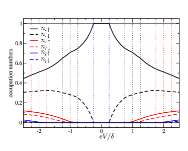
Figure 5: (color online) Occupation numbers of the spin, hole and particle states in the $3$-level Anderson model for symmetric coupling to the leads, $t_{\alpha n}=0.1\sqrt{U/\nu_{F}}$. For a clear separation of energy scales the temperature is chosen small $T/\delta=0.001$ and the levels are clearly separated $\delta^{\prime}/\delta=2$. The dashed lines indicate the transition energies $\{\pm g\mu_{B}B,\delta,\delta\pm g\mu_{B}B,\delta^{\prime},\delta^{\prime}\pm g\mu_{B}B\}$ in $\{$blue, black, red$\}$ for a finite magnetic field of $B/\delta=0.25$.

In Fig. 6 we show the same occupation numbers as in Fig. 5, but now calculated for different tunnel-couplings to the left lead. Again, the ground-state is partially depleted with increasing voltage, but due to the asymmetric couplings a clear asymmetry in bias is observed. For negative bias, only the $p$-states are being populated, due to a strong $|s\rangle\to|p\rangle$ (cotunneling) amplitude proportional to $t_{L2}t_{R3}=3$. The $|s\rangle\to|h\rangle$ amplitude is proportional to $t_{L1}t_{R2}=1/3$ and therefore only hardly pumped at all. For positive bias, the situation is reversed since $\langle p|H_{\mathrm{int}}|s\rangle\propto t_{L3}t_{R2}=1$ is now much smaller than $\langle h|H_{\mathrm{int}}|s\rangle\propto t_{R1}t_{L2}=3$, whereby it is $n_{h}$ which rises with voltage. Notice also that since $\langle h|H_{\mathrm{int}}|p\rangle=0$ there are no direct transitions between the two excited states, whereby an incipient occupation of $|h\rangle$, say, will be accompanied by a deletion of $|s\rangle$ and thereby further prohibit the pumping of $|p\rangle$.

For the asymmetric tunnel-couplings chosen for Fig. 6, one can also observe a population inversion at positive bias. That is, for $eV\gtrsim\delta+g\mu_{B}B$, $n_{h\uparrow}$ increases rapidly and stays larger than the ground-state occupation $n_{s\uparrow}$ for an extended bias-range. The positive bias demands electrons to predominantly jump from the left lead onto the dot and from the dot into the right lead. Therefore, $t_{L2}\gg t_{L1}$ will make the $|s\rangle\to|h\rangle$ much more likely than the $|h\rangle\to|s\rangle$ transition at positive bias and the dot gets stuck in the excited state $|h\rangle$. As we shall argue later, this excited state does not sustain as high a current as the ground state and therefore this population inversion will in fact lead to regions of negative differential conductance (NDC).

The ’direct’ threshold for populating $|h,\uparrow\rangle$, say, is given by $eV=\delta$. Nevertheless, from Fig. 6 it is seen that $n_{h\uparrow}$ starts growing already at $eV=\delta-g\mu_{B}B$. This slightly lower ’indirect’ threshold is due to a cascade effect in which $|s,\downarrow\rangle$ is populated for $V>g\mu_{B}B$ and from there the threshold to $|h,\uparrow\rangle$ is now only $\delta-g\mu_{B}B$ instead of $\delta$. Further cascade effects are observed at $eV=\delta$ (instead of the direct threshold $\delta+g\mu_{B}B$) which is the threshold for the transition $|s,\downarrow\rangle\to|h,\downarrow\rangle$. A similar effect for $n_{p,\sigma}$ is observed at negative bias, with indirect thresholds already at $eV=-(\delta^{\prime}-g\mu_{B}B)$ and $eV=-\delta^{\prime}$. Notice that these effects are just barely visible for symmetric couplings as in Fig. 5. As we shall see in the next subsection, these cascade effects show up as small steps in the nonlinear conductance.

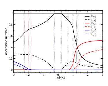
Figure 6: (color online) Occupation numbers of the spin, hole and particle states in the $3$-level Anderson model for non-symmetric coupling to the leads, i.e. $t_{L2}/t_{Rn}=3$, $t_{L3}/t_{Rn}=1$ and $t_{L1}/t_{Rn}=1/3$ where $t_{Rn}=0.1\sqrt{U/\nu_{F}}$. With the same finite magnetic field $B/\delta=0.25$, level splitting $\delta^{\prime}/\delta=2$ and temperature $T/\delta=0.01$ as in Fig. 5 we observe an occupation inversion around $eV\approx\delta+B$ since $n_{h\uparrow}$ becomes higher occupied than the ground state $n_{s\uparrow}$. This blocking of transitions and the cascade effect appearing at $\delta^{(^{\prime})}-g\mu_{B}B$ are discussed in the main text. Gridlines refer to various thresholds: $\pm g\mu_{B}B$ (blue), $\{\delta,\delta\pm g\mu_{B}B\}$ (black), and $\{-\delta^{\prime},-\delta^{\prime}\pm g\mu_{B}B\}$ (red).

III.2 Cotunneling conductance

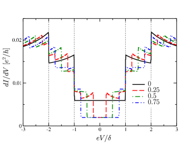
Figure 7: (color online) Dependence of the differential conductance $dI/dV$ on the applied bias voltage in units of $eV/\delta$ for various strengths of the magnetic field $g\mu_{B}B/\delta=0,0.25,0.5,0.75$. The quantum dot is coupled symmetrically to the lead with the parameters given in Fig. 5. The kinks at $\pm(\delta-g\mu_{B}B)$ and $\pm(\delta^{\prime}-g\mu_{B}B)$ originate from the occupation of excited states due to the cascade effect.

In Fig. 7 we show the differential conductance for the same parameter set as in Fig. 5. As expected, we find a step in $dI/dV$ whenever a new level enters the voltage window. Furthermore, as pointed out in Refs. Wegewijs:01, ; Paaske:04a, , the voltage-dependence of the nonequilibrium occupation numbers promotes these conductance steps to pointed cusps. Since we are limiting our calculations to second order perturbation theory, these plots do not take into account the possible Kondo-enhancement of these cusps. Nevertheless, the tendency is known from previous calculations: each cusp in the differential conductance to second order is logarithmically enhanced Paaske:04a and these logarithmic divergences are contained roughly by the inverse life-time of the excited state involved in the relevant inelastic cotunneling process Paaske:04b ; Rosch .

III.2.1 Cascade induced side-peaks

Even for the symmetric couplings in Fig. 7, we observe extra steps reflecting the aforementioned cascade effect. For example, the red (dashed) curve with $g\mu_{B}B=0.25\delta$ shows extra steps both at $eV=\delta-g\mu_{B}B$ ($|s,\downarrow\rangle\to|h,\uparrow\rangle$) and at $eV=\delta^{\prime}-g\mu_{B}B$ ($|s,\downarrow\rangle\to|p,\uparrow\rangle$). Notice that the cascade effect is only visible for $B\not=0$, and disappears when $2\,g\mu_{B}B>\delta(\delta^{\prime})$ since $n_{h,\uparrow}(n_{p,\uparrow})$ is then occupied before $n_{s,\downarrow}$.

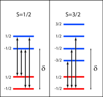
Figure 8: Comparison of direct and indirect transitions with a doublet groundstate and an excited doublet or quartet, respectively, at finite magnetic field. Cascade effect provides an indirect transition in the former, at energy $\delta-g\mu_{B}B$, which matches a direct transition in the latter.

More investigations are necessary in clarifying to what extent these cascade-features in the conductance will be enhanced by the Kondo-effect, but even a small additional step as seen in Fig. 7 can have important bearings for interpreting experiments in which the internal dot, or molecule states are not known in advance. Judging from the magnetic field dependence, the three transitions at $eV={\delta-g\mu_{B}B,\delta,\delta+g\mu_{B}B}$ seen in Fig. 7 (imagine for a moment that $\delta^{\prime}\gg\delta$) could in fact be misinterpreted as direct transitions between a spin-doublet ground state and an excited S=3/2 state, as illustrated by the energy-diagrams in Fig. 8. This example shows that a spin-spectrum read off from B-dependent inelastic cotunneling-lines in a diamond-plot ($dI/dV$ vs. $V_{g}$ and $V_{sd}$) should be interpreted with some care, especially when enhancing the lines by plotting higher derivatives of the current.

III.2.2 Negative differential conductance

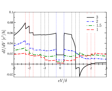
Figure 9: (color online) Differential conductance $dI/dV$ of the non-symmetric 3-level Anderson model with $3$ electron for the parameters given in Fig. 6. The four different set of parameters correspond to the ratio of $t_{L2}/t_{Rn}=\{3,2,1.5,1\}$ with $t_{L1}/t_{Rn}=1/(t_{L2}/t_{Rn})=\{1/3,1/2,2/3,1\}$, respectively. The parameter set with $t_{L2}/t_{Rn}=3$ and $t_{L1}/t_{Rn}=1/3$ corresponding to Fig. 6 shows NDC at the voltage values corresponding to an inversion of occupation probabilities.

In Fig. 9 we plot the conductance for the parameters used in Fig. 6 and with varying values for the tunneling amplitudes from the left lead to orbitals 1 and 2, respectively. As in Fig. 6, we observe a pronounced asymmetry in bias-voltage, and with the largest difference in couplings to orbitals 1 and 2 (black/solid curve), we observe a sudden drop to negative differential conductance for $eV\gtrsim\delta$. As mentioned before, the NDC is driven by the population inversion between $|s\rangle$ and $|h\rangle$. As argued in the previous section, the positive bias drives the dot into the excited state $|h\rangle$, and since (for these parameters) this state leads to a lower current than $|s\rangle$, the current decreases and we observe the NDC. The poor cotunneling across the dot in the state $|h\rangle$ is a simple consequence of the double occupancy of the well-coupled orbital 2, which demands that orbital 2 is emptied to the right lead before it can be filled from the left, thus making use of the strong coupling $t_{L2}=3$. In contrast, starting in $|s\rangle$ one can also fill in an electron in orbital 2 from the left lead first and then tunnel out into the right lead from either orbital 2 or from orbital 1, thus allowing more current-carrying tunneling processes involving $t_{L2}=3$.

Thus a sufficiently strong difference in coupling to two of the orbitals will cause a population inversion with a concomitant decrease in the current as bias is increased. For intermediate coupling asymmetry, we see from the other curves in Fig. 9 that the NDC disappears while an asymmetry in bias remains.

IV Discussion of experiments

IV.1 Experiments on Carbon Nanotube

The data shown in Fig. 3 were recorded on the same sample as was discussed in Ref. Paaske:06, . In fact, this is the neighboring charge-state to the even number occupied state studied in that work. In Ref. Paaske:06, , some of the present authors obtained a very gratifying fit to the inelastic cotunneling line reflecting a strong transition from singlet ground- to an excited triplet state. In particular, it was argued that the very sharp cotunneling line could only arise from the joint effect of nonequilibrium pumping (finite-bias occupations) of the triplet state and substantial logarithmic enhancements from the nonequilibrium Kondo-effect.

As already stated, we shall not embark on higher order perturbation theory in this paper, which means that we should not expect to obtain any quantitative agreement with the data in Fig. 3. Nevertheless, since basically all parameters were fixed by the fit in Ref. Paaske:06, , we shall assume that these remain largely unchanged when passing on to the neighboring charge-state and use them as input for a numerical evaluation of the nonlinear conductance there. The result is shown in Fig. 10 and the gross features such as bias-voltage asymmetry and B-field splittings match those of Fig. 3 quite well, albeit with a complete lack of sharp finite-bias peaks, as expected. The parameters from Ref. Paaske:06, were tunnel couplings of the two lowest lying levels of $\{t_{L1},t_{L2},t_{R1},t_{R2}\}=\{0.032,0.028,0.108,0.063\}\sqrt{U/\nu_{F}}$ (see Fig. 4 in Ref. Paaske:06, ), an orbital splitting of $\delta\approx 1.5$ meV, a charging energy of $U\approx 3.0$ meV, and a higher lying level at $\delta^{\prime}=\Delta-\delta\approx 3.1$ meV, $\Delta$ being the single-particle level spacing in the nanotube. Since $\delta^{\prime}\gtrsim U$, charge-excitations set in before orbital 3 is reached and this latter orbital is therefore not included in the calculation.

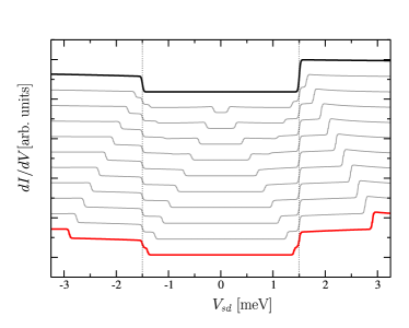
Figure 10: Modeling of the CNT QD analyzed in Ref. Paaske:06, as measured in the neighboring diamond, i.e. Fig. 3, where orbital scattering is observed at $\delta=1.5$ meV. Further parameters of the plot are $\{t_{L1},t_{L2},t_{R1},t_{R2}\}=\{0.032,0.028,0.108,0.063\}\sqrt{U/\nu_{F}}$, $B=0,0.14,\ldots 1.4\$meV, and $T=81$mK $\sim 0.008$meV. The conductance is given in arbitrary units and the curves are offset for clarity.

IV.2 Experiments on InAs-nanowires

The data shown in Fig. 2 constitute the first observation of Kondo-effect in InAs-nanowire quantum dots and were discussed by some of the present authors in Ref. Sand:06, . Already in that paper the 3-orbital model was invoked to explain the finite-bias peaks flanking the zero-bias Kondo peak and, as mentioned in the introduction, this experiment was the main motivation for this more detailed investigation of that model.

Apart from the zero-bias Kondo peak, it is the sharp finite-bias peaks which dominate these data: A very strong peak close to $eV=-1.4\$ meV together with a somewhat weaker peak close to $eV=1.1\$ meV (cf. Fig. 2). This asymmetry in bias-voltage was not addressed in Ref. Sand:06, , but as we shall argue it can readily be understood in terms of an asymmetry in tunneling amplitudes of orbital 2 to source and drain. The excited state giving the strong sequential tunneling line in the upper left corner of Fig. 11 (a) is ascribed to the excited 3-particle state with one electron in orbital 3 instead of orbital 2. This line connects to the inelastic cotunneling line at positive bias inside the N=3 diamond ($|s\rangle\to|p\rangle$ transition). From this we infer that $\delta^{\prime}\approx 1.1\$meV. Notice that a sequential tunneling line corresponding to a transition from the N=2 ground-state to the N=3 $|h\rangle$-state is only possible to higher order in the tunneling amplitudes and is therefore strongly suppressed in the experimental data. The inelastic cotunneling line at negative bias can now be ascribed to an (N=3) $|s\rangle\to|h\rangle$ transition at energy $\delta\approx 1.4\$meV. This is again consistent with the lower left corner of Fig. 11 (a) showing that this line connects to a very strong sequential tunneling line which must correspond to a transition from the N=4 ground-state to the N=3 $|h\rangle$-state. At this point it is the (N=3) $|p\rangle$-state which is not directly coupled to the N=4 ground-state and hence suppressed in the data.

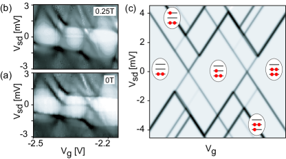
Figure 11: (a) and (b) Plot of $dI/dV$ vs. gate, and bias-voltage, for the InAs-wire quantum dot with $B=0$ T and $0.25$ T, respectively. Strong tunnel-coupling perturb the Coulomb-blockade diamond and particularly strong sequential tunneling lines are clearly present (thick dark lines) in the region with a mixture of 2 and 3 electrons on the dot. c) Calculation of the sequential tunneling lines from solving semiclassical rate-equations (conductance in arbitrary units) bringing out some of the main lines and indicating the states which are involved in the dominant transitions and which are involved in the cotunneling for $N=3$. Parameters are $\delta=1.4$ meV, $\delta^{\prime}=1.1$ meV, $T=300$mK, $U=3$ meV, $t_{L1}=t_{R1}=t_{L3}=t_{R3}=1$, $t_{L2}=0.4$, and $t_{R2}=2.5$.

In Fig. 11 (c), we show the result of solving a set of semiclassical rate-equations. The dark lines correspond to high conductance (arbitrary units) due to sequential tunneling only. We do not attempt a $6$ parameter fit of Fig. 11 (a), and tunneling amplitudes are therefore chosen with a very simple asymmetry, assuming that only orbital $2$ is coupled in a special way. This choice of parameters captures some, but not all, of the gross features of the data in Fig. 11 (a).

The question remains why there is only one and not two inelastic cotunneling peaks at both positive and negative bias. As demonstrated by the calculation shown in Fig. 12, however, the observed asymmetry in bias-voltage can be understood quite simply as orbital 2 being asymmetrically coupled to the source and drain electrodes. Notice that it is the nearly equidistant levels in the InAs-wire quantum dot which prompts us to incorporate the effects of both $h$ and $p$ excited states. For asymmetric couplings the $\delta^{\prime}=1.1$meV and $\delta=1.4$meV peaks in Fig. 12 dominate for positive and negative voltages, respectively, in contrast to symmetric coupling where both can be observed. The small steps observed for zero temperatue (blue/solid curve) are washed out for large temperature smearing (red/dashed curve) and the nonlinear conductance is now asymmetric with respect to voltage. For a larger difference in the effective $\delta$ and $\delta^{\prime}$, as is typical for carbon nanotube quantum dots where $\delta$ would be the subband-splitting and $\delta^{\prime}$ would be of the order of the single-particle level-spacing ($\Delta=\delta^{\prime}+\delta$), the $|p\rangle$ state would most often be masked by charge-fluctuations, i.e. $\delta^{\prime}$ will often be comparable to the charging-energy, $E_{C}$.

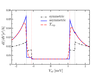
Figure 12: (color online) Plot of $dI/dV$ vs. bias voltage, $V$, calculated within second order perturbation theory. Parameters are chosen so as to approximately match the voltage asymmetry brought out by the experiment (compare Fig. 11). Parameters are $B=0$, $\delta=1.4$ meV, $\delta^{\prime}=1.1$ meV and $T=0.001$ meV (blue/solid curve). The black (dashed-dotted) curve corresponds to all equal tunneling amplitudes and the red (dashed) curve is the same as the blue (solid) but with temperature corresponding to the experiment ($T_{\mathrm{exp}}=300$mK$\sim 0.025$meV).

As demonstrated recently in the experiment by Csonka et al. Csonka:08 , the strong spin-orbit coupling in InAs can give rise to very different g-factors for neighboring quantum dot orbitals or energy-levels. In that experiment this was brought out particularly clear by a modulation of the orbitals by an additional top-gate. Fixing the top-gate voltage and adjusting the back-gate, it was shown that two neighboring levels could have g-factors of 1.9 and 10, respectively. It is interesting to note that such a difference in g-factors would give rise to an apparent $B$-dependence of the level-spacings. In our model, we would expect the following $B$-dependent inelastic cotunneling thresholds:

$${\tilde{\delta}}(B) =E_{h\uparrow}-E_{s\uparrow}=\delta+(g_{2}-g_{1})\mu_{B}B/2,$$

$${\tilde{\delta}}^{\prime}(B) =E_{p\uparrow}-E_{s\uparrow}=\delta^{\prime}+(g_{2}-g_{3})\mu_{B}B/2.$$

In Ref. Sand:06, , a detailed investigation of the splitting of both the zero-bias Kondo peak and the finite(positive)-bias cotunneling peak with magnetic field indeed revealed two different g-factors. Interpreting the finite-bias cotunneling as above, we can thus infer from Ref. Sand:06, that orbital 2 has $g_{2}=7.7$ and orbital 3 has $g_{3}=8.5$. This difference is rather small and would cause a largely negligible shift of roughly 0.02 meV of $\delta^{\prime}$ at largest applied fields (0.9 Tesla). In Fig. 13 we show the result of a calculation with slightly different g-factors by a factor of $2$. This is the cause of the slight shift of the main kink in the blue (solid) curve to a value above $eV=\delta$. The observation of such $B$-dependent cotunneling thresholds thus provides an interesting consistency check on the difference in g-factors of two neighboring orbitals.

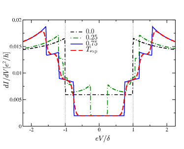
Figure 13: (color online) Plot of $dI/dV$ vs. bias voltage, $V$, calculated within second order perturbation theory for symmetric coupling to the leads and neglecting the particle state ($\delta^{\prime}>E_{C}$). The $g$-factors are different for the two involved levels: $g_{2}=2g_{1}$. The orbital peak moves towards higher voltages such as $\sim(1-g_{1}/g_{2})g_{2}\mu_{B}B/2$ with increasing magnetic field $g_{2}\mu_{B}B/\delta=\{0,0.25,0.75\}$. The red (dashed) curve at $g_{2}\mu_{B}B/\delta=0.75$ illustrates that the shift is also observable at a temperature corresponding to the experiment ($T_{\mathrm{exp}}=300$mK$\sim 0.025$ meV).

In closing, we note that the diamond-plot in the upper left panel of Fig. 11 has a few strong-coupling irregularities which we do not address in this paper. First of all, the inelastic cotunneling lines display a slight dependence on gate-voltage. This is a feature which was investigated in detail for a carbon nanotube quantum dot in Ref. Holm:08, , where it was explained in terms of second order tunneling-renormalization with energy denominators depending on gate-voltage. Second, the inelastic cotunneling line at positive bias, which we assigned to the excited $p$-state, appears to continue straight through the sequential tunneling region mixing N=3 and N=4 states. At this point we merely speculate that this is related to a very strongly coupled orbital 3, which might allow the partially populated N=4 states to conduct via virtual transitions to the N=5 state. How, and if, this would work out in detail will be assessed in future work.

V Conclusions

In this paper we have analyzed the inelastic cotunneling spectroscopy of a system with three electrons distributed among three orbitals. Starting from the 3-orbital Anderson model in the Coulomb blockade regime, we have projected out charge-fluctuations and derived an effective cotunneling (Kondo) model describing elastic as well as inelastic tunneling induced transitions between different orbital and spin states of the impurity or quantum dot in the N=3 charge-state. By treating all tunnel couplings independently we can study asymmetric behavior inherent to most of the experimental samples.

All calculations were performed within second order nonequilibrium perturbation theory, and the bias dependent nonequilibrium occupations of the impurity-states were shown to give rise to marked cusps at voltages matching the different transitions. We demonstrate how a bias induced cascade in the occupations can lead to indirect transitions between two excited states. Furthermore, we find that certain asymmetries in the tunneling amplitudes of the three orbitals can lead to a population inversion, which in turn can be accompanied by lines of negative differential (cotunneling) conductance (NDC).

We have revisited the carbon nanotube data from Ref. Paaske:06, with focus on an odd occupied charge-state. Importing the tunnel-couplings inferred from Ref. Paaske:06, , we confirm the asymmetry in the conductance strength at positive and negative bias. These parameters lead to steps at finite-bias at the orbital transitions, and we believe that the experimentally observed peaks are mainly due to logarithmic enhancements from a nonequilibrium Kondo-effect.

We have also analyzed the InAs-wire data from Ref. Sand:06, in greater detail and provided an explanation of the bias-asymmetry in peak-positions. This was understood as a slight difference in the two level-spacings together with an asymmetry in the tunnel-coupling of orbital 2 to source and drain electrodes. This asymmetry in couplings was roughly consistent with the overall stability diagram for the N=3 diamond, as confirmed by a semiclassical rate-equation calculation. Finally, we have pointed to an additional consequence of strong spin-orbit coupling in the InAs-wires, namely the apparent $B$-dependence of the level-spacing caused by different g-factors for different orbitals. In the present experiment this difference was too small to give a noticeable effect, but with differences as quoted in Ref. Csonka:08, it should be a pronounced effect . Possible further influence of strong spin-orbit coupling on the cotunneling spectroscopy of inelastic spin and orbital transitions constitutes an interesting problem on its own right and will be addressed in a separate publication.

Appendix A Schrieffer-Wolff transformation and Coupling Constants

In this work we concentrate on the physics inside a Coulomb diamond where the 3-level quantum dot is occupied by exactly three electrons. All virtual processes to two or four electron states can be treated perturbatively and lead to a Kondo-like interaction and potential scattering terms.

Using a Schrieffer-Wolff transformation Schrieffer:66 we find to second order in the tunneling Hamiltonian $H_{tun}$ the interaction Hamiltonian

$$H_{\mathrm{int}} =\sum_{\begin{subarray}{c}\alpha,\beta;n,m\\ \sigma,\sigma^{\prime}\end{subarray}}\Big{\{}t_{\alpha m}t^{*}_{\beta n}c^{\dagger}_{\alpha\sigma}f^{\phantom{\dagger}}_{m\sigma}\frac{1}{E_{a\sigma}-E_{4e^{-}}}f^{\dagger}_{n\sigma^{\prime}}c^{\phantom{\dagger}}_{\beta\sigma^{\prime}}$$

$$\qquad+t^{*}_{\alpha m}t_{\beta n}f^{\dagger}_{m\sigma}c^{\phantom{\dagger}}_{\alpha\sigma}\frac{1}{E_{a\sigma}-E_{2e^{-}}}c^{\dagger}_{\beta\sigma^{\prime}}f^{\phantom{\dagger}}_{n\sigma^{\prime}}\Big{\}}.$$

which can be rewritten as

$$H_{\mathrm{int}} =\sum_{\begin{subarray}{c}\alpha,\beta;n,m\\ \sigma,\sigma^{\prime}\end{subarray}}\left\{\frac{t_{\alpha m}t_{\beta n}^{*}}{\varepsilon_{n}+3U}-\frac{t_{\beta n}^{*}t_{\alpha m}}{\varepsilon_{m}+2U}\right\}c_{\alpha\sigma}^{\dagger}c_{\beta\sigma^{\prime}}^{\phantom{\dagger}}f_{n\sigma^{\prime}}^{\dagger}f_{m\sigma}$$

$$-\sum_{\begin{subarray}{c}\alpha,\beta;n,m\\ \sigma,\sigma^{\prime}\end{subarray}}\delta_{n,m}\delta_{\sigma\sigma^{\prime}}\frac{t_{\alpha m}t_{\beta n}^{*}}{\varepsilon_{n}+3U}c_{\alpha\sigma}^{\dagger}c_{\beta\sigma^{\prime}}^{\phantom{\dagger}}$$ (23)

The Kondo exchange interaction for the levels $n,m=\{1,2,3\}$ and thus for the orbital states $a,b=\{s,h,p\}$ can straightforwardly be read off this expression

$$J_{\alpha\beta}^{11} =J_{\alpha\beta}^{hh}=2\Big{(}\frac{t_{\alpha 1}t_{\beta 1}^{*}}{\varepsilon_{1}+3U}-\frac{t_{\beta 1}^{*}t_{\alpha 1}}{\varepsilon_{1}+2U}\Big{)}$$

$$J_{\alpha\beta}^{22} =J_{\alpha\beta}^{ss}=2\Big{(}\frac{t_{\alpha 2}t_{\beta 2}^{*}}{\varepsilon_{2}+3U}-\frac{t_{\beta 2}^{*}t_{\alpha 2}}{\varepsilon_{2}+2U}\Big{)}$$

$$J_{\alpha\beta}^{33} =J_{\alpha\beta}^{pp}=2\Big{(}\frac{t_{\alpha 3}t_{\beta 3}^{*}}{\varepsilon_{3}+3U}-\frac{t_{\beta 3}^{*}t_{\alpha 3}}{\varepsilon_{3}+2U}\Big{)}$$

$$J_{\alpha\beta}^{12} =J_{\alpha\beta}^{sh}=2\Big{(}\frac{t_{\alpha 2}t_{\beta 1}^{*}}{\varepsilon_{1}+3U}-\frac{t_{\beta 1}^{*}t_{\alpha 2}}{\varepsilon_{2}+2U}\Big{)}$$

$$J_{\alpha\beta}^{21} =J_{\alpha\beta}^{hs}=2\Big{(}\frac{t_{\alpha 1}t_{\beta 2}^{*}}{\varepsilon_{2}+3U}-\frac{t_{\beta 2}^{*}t_{\alpha 1}}{\varepsilon_{1}+2U}\Big{)}$$

$$J_{\alpha\beta}^{32} =J_{\alpha\beta}^{ps}=2\Big{(}\frac{t_{\alpha 2}t_{\beta 3}^{*}}{\varepsilon_{3}+3U}-\frac{t_{\beta 3}^{*}t_{\alpha 2}}{\varepsilon_{2}+2U}\Big{)}$$

$$J_{\alpha\beta}^{23} =J_{\alpha\beta}^{sp}=2\Big{(}\frac{t_{\alpha 3}t_{\beta 2}^{*}}{\varepsilon_{2}+3U}-\frac{t_{\beta 2}^{*}t_{\alpha 3}}{\varepsilon_{3}+2U}\Big{)}$$

which leads to the interaction Hamiltonian as defined in the main text. Note that the potential scattering which changes the orbital index is of the same strength as the spin Kondo scattering with an orbital change, $J^{h/p,s}_{\alpha\beta}$. In lowest order, i.e. involving two hopping processes, there is no transition between the hole and the particle state and we assume for the following

$$J_{\alpha\beta}^{hp}=J_{\alpha\beta}^{ph}=0.$$

Furthermore we disregard a constant shift due to the following potential scattering contribution

$$H_{pot.scat}= -\frac{1}{2}\sum\limits_{\alpha\beta}{\cal C}_{\alpha\beta}\Big{(}\sum_{\sigma}c_{\alpha\sigma}^{\dagger}c_{\beta\sigma}\Big{)}$$

since it is negligible small at the particle-hole symmetric point $\varepsilon_{2}=-5/2\ U$,

$${\cal C}_{\alpha\beta}= \Big{(}\frac{t_{\alpha 1}t_{\beta 1}^{*}}{\varepsilon_{1}+3U}+\frac{t_{\beta 1}t_{\alpha 1}^{*}}{\varepsilon_{1}+2U}\Big{)}$$

$$+\Big{(}\frac{t_{\alpha 2}t_{\beta 2}^{*}}{\varepsilon_{2}+3U}+\frac{t_{\beta 2}t_{\alpha 2}^{*}}{\varepsilon_{2}+2U}\Big{)}+\Big{(}\frac{t_{\alpha 3}t_{\beta 3}^{*}}{\varepsilon_{3}+3U}+\frac{t_{\alpha 3}t_{\beta 3}^{*}}{\varepsilon_{3}+2U}\Big{)}$$

$$= t_{\alpha 1}t_{\beta 1}^{*}\frac{2\delta}{(U/2)^{2}-\delta^{2}}-t_{\alpha 3}t_{\beta 3}^{*}\frac{2\delta^{\prime}}{(U/2)^{2}-(\delta^{\prime})^{2}}.$$

This constant offset in the current of order $\delta/U^{2}$ is neglected in our calculation.

Appendix B Calculation of the Self Energies

The Green’s functions for the orbital states $a,b=\{s,h,p\}$ are calculated by an expansion in the interaction Hamiltonian

$$\mathcal{G}_{ab,\sigma\sigma^{\prime}}(\tau,\tau^{\prime})=-\mathrm{i}\left\langle T_{C_{K}}d_{a\sigma}^{\phantom{\dagger}}(\tau)d_{b\sigma^{\prime}}^{\dagger}(\tau^{\prime})\right\rangle_{0}$$

$$+(-\mathrm{i})^{2}\int_{C_{K}}\mathrm{d}\tau_{1}\left\langle T_{C_{K}}d_{a\sigma}^{\phantom{\dagger}}(\tau)H_{\mathrm{int}}(\tau_{1})d_{b\sigma^{\prime}}^{\dagger}(\tau^{\prime})\right\rangle_{0}$$

$$+\frac{(-\mathrm{i})^{3}}{2}\int_{C_{K}}\mathrm{d}\tau_{1}\mathrm{d}\tau_{2}\left\langle T_{C_{K}}d_{a\sigma}^{\phantom{\dagger}}(\tau)H_{\mathrm{int}}(\tau_{1})H_{\mathrm{int}}(\tau_{2})d_{b\sigma^{\prime}}^{\dagger}(\tau^{\prime})\right\rangle_{0}$$

$$+\mathcal{O}(H_{\mathrm{int}}^{3})$$ (24)

The linear order does not contribute since it contains the expectation value of $\langle\mathbf{s}_{\alpha\beta}\rangle$ which is zero if the spin in the leads are not polarized. In the case of ferromagnetic leads this order has to be taken into account, but in our setup the leading order is second order in the coupling.

We get contributions from the spin part of the interaction Hamiltonian and of the potential scattering part. A mixing between both parts does not appear in second order due to the convolution of the leads contribution.

For example the spin part is given by (Einstein’s sum rule)

$$\mathcal{G} {}_{ab,\sigma\sigma^{\prime}}^{(2),\mathrm{Spin}}(\tau,\tau^{\prime})=\frac{\mathrm{i}}{2}\int\mathrm{d}\tau_{1}\mathrm{d}\tau_{2}\frac{1}{4}\boldsymbol{\tau}^{i_{1}}_{\sigma_{1}^{\prime}\sigma_{1}}\boldsymbol{\tau}^{i_{2}}_{\sigma^{\prime}_{2}\sigma_{2}}$$

$$\qquad\times\left\langle T_{\mathrm{C_{K}}}c^{\dagger}_{\alpha\sigma^{\prime}_{1}}(\tau_{1})c^{\phantom{\dagger}}_{\beta\sigma_{1}}(\tau_{1})c^{\dagger}_{\alpha^{\prime}\sigma^{\prime}_{2}}(\tau_{2})c^{\phantom{\dagger}}_{\beta^{\prime}\sigma_{2}}(\tau_{2})\right\rangle_{0}$$

$$\qquad\times\left\langle T_{\mathrm{C_{K}}}d^{\phantom{\dagger}}_{a\sigma}(\tau)J_{\alpha\beta}^{a_{1}b_{1}}\mathbf{S}^{i_{1}}_{a_{1}b_{1}}(\tau_{1})J_{\alpha^{\prime}\beta^{\prime}}^{a_{2}b_{2}}\mathbf{S}^{i_{2}}_{a_{2}b_{2}}(\tau_{2})d_{b\sigma^{\prime}}^{\dagger}(\tau^{\prime})\right\rangle_{0}$$

The conduction electron spins contract to

$$\boldsymbol{\tau}_{\sigma^{\prime}\sigma}\boldsymbol{\tau}_{\sigma\sigma^{\prime}}\delta_{\alpha^{\prime}\beta}\delta_{\alpha\beta^{\prime}}G_{\beta\sigma^{\prime}}^{(0)}(\tau_{1},\tau_{2})G_{\alpha\sigma}^{(0)}(\tau_{2},\tau_{1}).$$

Since the leads are not magnetic, the conduction electron Green’s functions does not depend on spin and the sum over the spins acts only on the $\tau$-matrices and we can thus introduce the conduction electron spin susceptibility $\chi_{\alpha\beta}(\tau_{2},\tau_{1})=G_{\alpha}^{(0)}(\tau_{2},\tau_{1})G_{\beta}^{(0)}(\tau_{1},\tau_{2})$.

As discussed before there can in general be solutions with $a\not=b$ which we neglect in this setup Koerting:08 . The result for the diagonal Greens’s function yields finally the second order self energy by comparison with the Dyson series:

$$\Sigma_{a\sigma}(\tau_{1},\tau_{2}) =\frac{1}{16}\Big{(}J_{\alpha\beta}^{ab}J_{\beta\alpha}^{ba}+J_{\alpha\beta}^{ba}J_{\beta\alpha}^{ab}\Big{)}\chi_{\alpha\beta}(\tau_{2},\tau_{1})$$

$$\quad\big{[}2\boldsymbol{\tau}_{\sigma\sigma^{\prime}}\boldsymbol{\tau}_{\sigma^{\prime}\sigma}+\delta_{\sigma,\sigma^{\prime}}{\cal P}_{a,b}\big{]}G_{b\sigma^{\prime}}(\tau_{1},\tau_{2})$$

$$+\Sigma_{a\sigma}^{\mathrm{el}}(\tau_{1},\tau_{2})$$

where the inelastic and elastic potential scattering contributions are defined as

$${\cal P}_{ab} =\big{(}\delta_{a,s}\delta_{b,p}+\delta_{b,s}\delta_{a,p}+\delta_{a,s}\delta_{b,h}+\delta_{b,s}\delta_{a,h}\big{)}$$

$$\Sigma_{a\sigma}^{\mathrm{el}}(\tau_{1},\tau_{2}) =\frac{1}{8}\sum_{\tilde{a}}J_{\alpha\beta}^{\tilde{a}\tilde{a}}J_{\beta\alpha}^{\tilde{a}\tilde{a}}\chi_{\alpha\beta}(\tau_{2},\tau_{1})$$

$$\big{(}\delta_{\tilde{a},p}\delta_{a,h}+\delta_{\tilde{a},s}\delta_{a,p}+\delta_{\tilde{a},p}\delta_{a,s}\big{)}G_{a\sigma}(\tau_{1},\tau_{2})$$

Note that in the rate equation $\Sigma_{a\sigma}^{el}$ does not contribute since it does not contain transitions between states.

The self-energy components needed in Eq. (19) are now readily obtained from analytical continuation using the Langreth rules.

References

• (1) D. Goldhaber-Gordon, H. Shtrikman, D. Mahalu, D. Abusch-Magder, U. Meirav and M. A. Kastner, Nature 391, 156 (1998).
• (2) S. M. Cronenwett, T. H. Oosterkamp and L. P. Kouwenhoven, Science 281, 540 (1998).
• (3) W. G. van der Wiel, S. De Franceschi, T. Fujisawa, J. M. Elzerman and S. Tarucha, Science 289, 2105 (2000).
• (4) J. Nygård, D. H. Cobden and P. E. Lindelof, Nature 408, 342 (2000).
• (5) T. Sand Jespersen, M. Aagesen, Claus Sørensen, Poul Erik Lindelof, and Jesper Nygård, Phys. Rev. B, 74, 233304 (2006).
• (6) D. M. Zumbühl, C. M. Marcus, M. P. Hanson and A. C. Gossard, Phys. Rev. Lett. 93, 256801 (2004).
• (7) B. Babic, T. Kontos and C. Schönenberger, Phys. Rev. B 70, 235419 (2004).
• (8) J. Paaske, A. Rosch, P. Wölfle, N. Mason, C. M. Marcus and J. Nygård, Nature Physics 2, 460 (2006).
• (9) J. V. Holm, H. I. Jørgensen, K. Grove-Rasmussen, J. Paaske, K. Flensberg and P. E. Lindelof, Phys. Rev. B 77, 161406(R) (2008).
• (10) S. Csonka, L. Hofstetter, F. Freitag, S. Oberholzer, C. Schonenberger, T. S. Jespersen, M. Aagesen, and J. Nygard, Nano Lett. 8 (11), 3932 (2008).
• (11) E. A. Osorio, K. O’Neil, M. R. Wegewijs, N. Stuhr-Hansen, J. Paaske, T. Bjornholm, H. S. J. van der Zant, Nano Letters 7, 3336, 2007.
• (12) N. Roch, S. Florens, V. Bouchiat, W. Wernsdorfer and F. Balestro, Nature 453, 633 (2008).
• (13) J. R. Schrieffer and P. A. Wolff, Phys. Rev. 149, 491 (1966).
• (14) O. Parcollet, and C. Hooley, Phys. Rev. B 66, 085315 (2002).
• (15) J. Paaske, A. Rosch, and P. Wölfle, Phys. Rev. B 69, 155330 (2004).
• (16) J. Rammer and H. Smith, Rev. Mod. Phys. 58, 323 (1986).
• (17) H. Haug and A.-P. Jauho, Quantum Kinetics in Transport and Optics of Semiconductors, Springer Series in Solid-State Science, Springer-Verlag, (1996).
• (18) A. A. Abrikosov, Physics 2, 5 (1965).
• (19) V. Koerting, J. Paaske, and P. Wölfle, Phys. Rev. B 77, 165122 (2008).
• (20) M. R. Wegewijs & Yu. V. Nazarov, cond-mat/0103579.
• (21) J. Paaske, A. Rosch, J. Kroha and P. Wölfle, Phys. Rev. B 70, 155301 (2004).
• (22) A. Rosch, J. Paaske, J. Kroha, and P. Wölfle, Phys.Rev. Lett. 90, 076804 (2003); J. Phys. Soc. Jpn. 74, 118 (2005).